Towards Optimal One Pass Large Scale Learning with Averaged Stochastic Gradient Descent

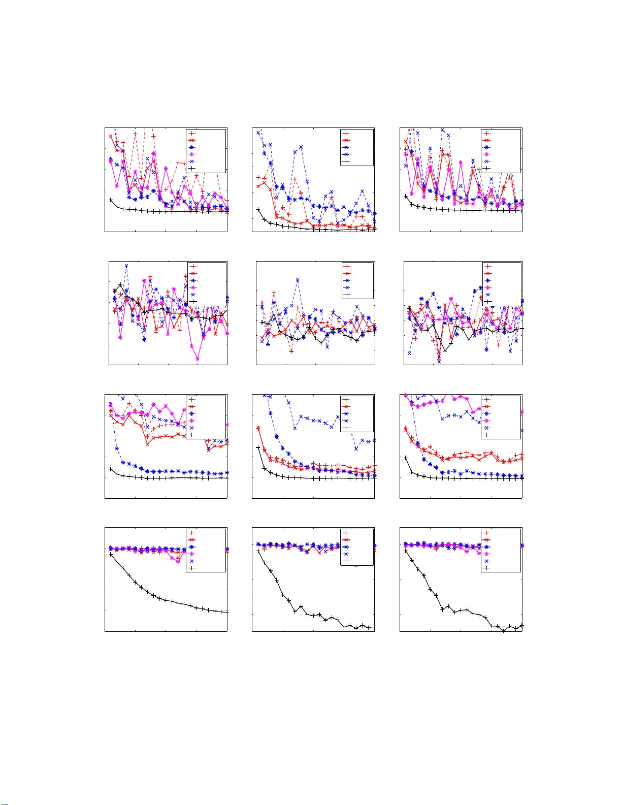
T o w ards Optimal One P ass Large Scale Learning with Av eraged Sto c hastic Gradien t Descen t W ei Xu email weix u@fb.com F ac eb o ok, Inc. 1 1601 S. California Ave Palo A l to, CA 94304, USA Editor: Abstract F or large scal e learning problems, it is desirable if we can obtain the optimal mo del parameters by going t h rough the data in only one pass. Poly ak and Juditsky (1992) sho wed that asymptoticall y the test p erformance of the simple av erage of th e parameters obtained by stochasti c gradien t descent (SGD) is a s go o d as that of the parameters whic h minimize th e empirical cost. How ever, to our know ledge, d espite its optimal asymp t otic con vergence rate, a vera ged SGD (ASGD) received little attentio n in recen t research on large scale learning. One p ossible reason is that it may take a prohibitiv ely large number of training samples for ASGD to reac h its asymptotic region for most real problems. In this paper, we present a fi nite sample analysis for th e method of P olyak and Juditsky (1992). Our analysis sho ws that it indeed usually takes a huge n umb er of samples for ASGD to reach its asymptotic region for imp roperly c hosen learning rate. More imp ortantly , based o n our analysis , we prop ose a simple w ay to properly set learning rate s o that it takes a reasonable amount of data for AS GD to reach its asymp totic region. W e compare A SGD using our prop osed learning rate with o t h er wel l kno wn algorithms for tra ining large scale linear classifiers. The experiments clearly sho w the superiority of A SGD. Keywords: stochastic gradien t descen t, large scale learning, supp ort vector machines, sto chastic optimization 1. In tro duction F or pr e dic tio n pro blems, w e wan t to find a function f θ ( x ) with par a meter θ to pr edict the v alue of the outcome v ariable y given an observed vector x . Typically , the problem is formulated as an optimization problem: θ ∗ t = arg min θ 1 t t X i =1 ( L ( f θ ( x i ) , y i ) + R ( θ )) (1) where t is the num b er o f data p o ints, θ ∗ t is the par ameter that minimize the e mpir ical cost, ( x i , y i ) are the i th training example, L ( s, y ) is a lo ss function which g ives small v alue if s is a go o d prediction for y , and R ( θ ) is a re g ularizatio n function for θ which typically gives small v alue for s mall θ . Some commonly used L ar e: max(0 , 1 − y s ) for supp o rt vector machine (SVM), 1 2 (max(0 , 1 − y s )) 2 for L2 SVM, and 1 2 ( y − s ) 2 for linear regres sion. So me commonly used reg ularizatio n functions are: L2 regular iz ation λ 2 k θ k 2 , and L1 regula rization λ k θ k 1 . F or large sca le machine lea rning problems, we need to deal with optimization pr o blems with millions or even billions of tr aining samples. The cla ssical optimization techniques such as interior po int metho ds o r conjuga te g radient descent hav e to go throug h a ll data po ints to just ev aluate the 1. Ma jor part of the work was done when the author was at NEC Labs America, Inc. 1 ob jective once. Not to say that they need to go through the whole data s e t many times in order to find the b est θ . On the o ther hand, sto chastic gr a dient descent (SGD) ha s be e n shown to hav e grea t promise for large sca le learning (Zha ng, 20 0 4; Ha zan et al., 2 006; Shalev- Shw artz et al., 2007; Bo ttou a nd Bousquet, 2008; Shalev-Shw ar tz a nd T ewari, 20 09; La ngford et al., 2009). Let d = ( x, y ) be one data sa mple, l ( θ, d ) = L ( f θ ( x ) , y ) + R ( θ ) b e the cost of θ for d , g ( θ , ξ ) = ∂ l ( θ ,d ) ∂ θ be the g radient function, and D t = ( d 1 , · · · , d t ) b e a ll the training samples a t t th step. The SGD metho d up dates θ a ccording to its sto chastic gr adient: θ t = θ t − 1 − γ t g ( θ t − 1 , d t ) (2) where γ t is learning rate at the t th step. γ t can b e either a scalar or a matrix . Let the exp ected loss o f θ ov er test da ta b e E ( θ ) = E d ( l ( θ , d )), the optimal parameter be θ ∗ = arg min θ E ( θ ), a nd the Hessian b e H = ∂ 2 E ( θ ) ∂ θ ∂ θ T    θ = θ ∗ . Note that θ t and θ ∗ t are random v ar iables dep ending o n D t . Hence bo th E ( θ t ) and E ( θ ∗ t ) are r andom v ariables depending o n D t . If γ t is a sc a lar, the be s t asymptotic conv erg e nce for the e x pe c ted exces s loss E D t ( E ( θ t )) − E ( θ ∗ ) is O ( t − 1 ), which is obtained by us ing γ t = γ 0 (1 + γ 0 λ 0 t ) − 1 , where λ 0 is the sma llest eig env alue of H and γ 0 is s o me co nstant. The asymptotic conv er gence rate of SGD can b e p otentially b enefit from using second or der infor mation (Bottou and Bousq uet, 2 008; Schraudolph et al., 20 07; Amari et a l., 2000). The optima l a symptotic conv erg e nce ra te is achiev e d by using matr ix v alued lea rning rate γ t = 1 t H − 1 . If this optimal matr ix step siz e is us ed, then asymptotically seco nd or der SGD is as go o d as explicitly optimizing the empirical los s. Mor e precisely , this means that b oth tE D t ( E ( θ t ) − E ( θ ∗ )) and tE D t ( E ( θ ∗ t ) − E ( θ ∗ )) conv erg e to a same p ositive cons tant. Since H is unknown in a dv ance, metho ds for adaptively estimating H is pr op osed (Bottou a nd Le C un, 2005; Amari et al., 200 0). How e ver, for high dimensiona l da ta se ts , maintaining a full matr ix H is to o co mputationally exp ensive. Hence v ar io us metho ds for approximating H hav e b een prop os ed (LeCun et al., 1998; Sc hra udolph e t al., 2007; Roux et al., 2008; Bordes et a l., 2009). Howev er, with the appr oximated H , the optimal co nv ergence ca nnot b e guar anteed. It is worth to po int o ut that most of the exis ting analy s is for sec ond order SGD is asymptotic, namely , that they do not tell how m uch da ta is needed for the algorithm to rea ch their a symptotic region. In order to a ccelerate the co nv ergence sp eed of SGD, averaged sto chastic g radient (ASGD) was prop osed in Poly ak and Juditsky (1992). F or ASGD, the running av er age ¯ θ t = 1 t P t j =1 θ j of the parameters obtained by SGD is us e d a s the estimato r for θ ∗ . Poly a k and Juditsky (19 92) showed a very nice result that ¯ θ t conv erg e s to θ ∗ as go o d as full s econd order SGD, which means that if there are enough training samples, ASGD can obtain the par ameter as go o d as the empirical optimal parameter θ ∗ t in just o ne pass of data. And another adv antage o f ASGD is that, unlik e second order SGD, ASGD is extremely easy to implement. Zhang (2 004); Nemirovski et al. (2009) gav e some nice non-a s ymptotic a nalysis for ASGD w ith a fixed learning r ate. Ho wever, the conv e r gence bo unds obtained by Zhang (20 04); Nemir ovski et al. (2009) are far less app ealing than that of Poly ak a nd Juditsky (199 2). Despite its nice prop erties , ASGD receives little a ttent io n in recent re s earch for online lar ge scale learning. The reas on for the lack of interest in ASGD mig ht b e that its p otential go o d conv ergence has not b een realized by r esearchers in rea l a pplica tions. Our ana lysis shows the ca use of this may due to the fact the ASGD needs a prohibitively lar ge amount o f data to reach a symptotics if lea rning rate is chosen ar bitr arily . A typical choice for the learning rate γ t is to ma ke it deceas e as fast as Θ ( t − c ) for s ome cons tant c . In this pap er, we assume a pa rticular form o f learning r ate schedule whic h satisfies this condition, γ t = γ 0 (1 + a γ 0 t ) − c (3) where γ 0 , a and c ar e so me constants. Base d on this form o f lea rning rate schedule, we provide non- asymptotic a nalysis of ASGD. O ur ana lysis shows that γ 0 and a should to b e prop er ly set according 2 to the curv ature o f the exp ected cost function. c should b e a problem indep endent constant. With our recip e for s etting the learning rate, we show that ASGD outp e rforms SGD if the data size is large enough for SGD to r each its asymptotic regio n. T o demonstrate the effectiveness of ASGD with the prop osed learning rate schedule, we apply ASGD for tr a ining linear cla ssification and r egressio n mo dels. W e c o mpare ASGD with other promi- nent lar ge sca le SVM solvers o n several b enchmark tasks. Our exp er iment a l results show the c lear adv antage o f ASGD. In the rest of the pap er, for matric e s X and Y , X ≤ Y means Y − X is p o s itive semi-definite, k x k A is defined a s √ x T Ax . W e will assume γ t = γ 0 (1 + aγ 0 t ) − c for s ome c o nstant γ 0 > 0, a > 0 and 0 ≤ c ≤ 1 in all the theorems and lemmas. Through out this pa per we denote ∆ t = θ t − θ ∗ and ¯ ∆ t = ¯ θ t − θ ∗ . T o help the reader fo cus on the ma in idea, we put mo st pr o ofs to the App endix. The pap er is organize d as fo llows: Section 2 establish s ome results on sto chastic linear equa- tion; Section 3 extends the re s ult to ASGD for quadratic loss functions; Section 4 works on gene r al non-quadra tic loss functions; Sec tio n 5 discusses so me implementation issues; Se c tion 6 shows ex- per imental results; Section 7 c o ncludes the pap er; and Appendix includes all the pro ofs. 2. Sto c hastic Linear Equation T o motiv ate the pr oblem, we first take a clos e lo ok a t the SGD up date (2). Let ¯ g ( θ ) = E ( g ( θ , d )) and the first order T a ylo r expansion of ¯ g ( θ ) around θ ∗ be Aθ − b , where A = ∂ ¯ g ( θ ) ∂ θ    θ = θ ∗ and b = Aθ ∗ − ¯ g ( θ ∗ ) = Aθ ∗ . Then g ( θ t − 1 , d ) ca n b e decomp os ed a s: g ( θ t − 1 , d ) = ( Aθ t − 1 − b ) + g ( θ ∗ , d ) + ( g ( θ t − 1 , d ) − g ( θ ∗ , d ) − ¯ g ( θ t − 1 )) + ( ¯ g ( θ t − 1 ) − Aθ t − 1 + b ) = ( Aθ t − 1 − b ) + ξ (1) t + ξ (2) t + ξ (3) t where ξ (1) t = g ( θ ∗ , d t ), ξ (2) t = g ( θ t − 1 , d t ) − g ( θ ∗ , d t ) − ¯ g ( θ t − 1 ) and ξ (3) t = ¯ g ( θ t − 1 ) − Aθ t − 1 + b . So the SGD upda te (2) can b e r e-written as θ t = θ t − 1 − γ t ( Aθ t − 1 − b + ξ (1) t + ξ (2) t + ξ (3) t ) (4) It is easy to see that ξ (1) t is martingale with resp ect to d t , i.e., E ( ξ (1) t | d 1 , · · · , d t − 1 ) = 0, a nd ha s ident ic a l distribution fo r differen t t . ξ (2) t is also martingale with resp ect to d t . Ho wev er , a s we will see in later sectio n, its magnitude dep ends on θ t − 1 − θ ∗ . If g ( θ , d ) is s mo oth, we have ξ (2) t = O ( k θ t − 1 − θ ∗ k ). F or s mo oth ¯ g ( θ ), we have ξ (3) t = o ( k θ t − 1 − θ ∗ k ). Both ξ (2) t and ξ (3) t are asymptotically negligible if suitable conditions are met. W e also note that ξ (3) t = 0 for quadra tic l ( θ , ξ ). By the ab ov e analys is, we first consider the following simple sto chastic approximation pro cedur e which ignor es ξ (2) t and ξ (3) t : θ t = θ t − 1 − γ t ( Aθ t − 1 − b + ξ t ) (5) ¯ θ t = 1 t t X i =1 θ i (6) where A is a p ositive definite matrix with the smallest eig env alue λ 0 and the lar gest eig e n v alue λ 1 , ξ t is martingale difference pr o cess, i.e ., E ( ξ t | ξ 1 , · · · , ξ t − 1 ) = 0, the v ar iance of ξ t is E ( ξ t ξ T t ) = S . W e will see that this a lgorithm can b e used to find the ro o t θ ∗ of equation Aθ = b Theorem 1 If γ 0 λ 1 ≤ 1 and (2 c − 1) a < λ 0 , then the estimator ¯ θ t in (6) satisfies: tE ( k ¯ θ t − θ ∗ k 2 A ) ≤ tr( A − 1 S ) + (2 c 0 + c 2 0 )(1 + aγ 0 t ) c − 1 c tr( A − 1 S ) + (1 + c 0 ) 2 γ 2 0 t k θ 0 − θ ∗ k 2 A − 1 3 wher e c 0 = ac (1 + acγ 0 ) ( λ 0 − max(0 , 2 c − 1) a ) The immediate co nc lus ion from Theorem 1 is the asy mptotic co nv ergence b ound of ¯ θ t . Corollary 2 ¯ θ t in (6) satisfies tE ( k ¯ θ t − θ ∗ k 2 A ) ≤ tr( A − 1 S ) + O ( t − (1 − c ) ) The ab ov e bound is consistent with Theo rem 1 in Polyak a nd Juditsky (1992) and is the bes t po ssible asymptotic convergence rate that ca n b e achiev ed by any alg o rithms (F abian, 19 73). How ever, we are more interested in the no n-asymptotic b ehavior of ¯ θ t . Corollary 3 If we cho ose a = λ 0 , it takes t = O (( λ 0 γ 0 ) − 1 ) samples for ¯ θ t in (6) to r e ach the asymptotic r e gion. A nd at this p oint, ¯ θ t b e gins to b e c ome b ett er than θ t . Pro of Let t = K λ 0 γ 0 , we hav e E ( k ¯ ∆ t k 2 A ) ≤ (1 + c 0 ) 2 K 2 k ∆ 0 k 2 A + λ 0 γ 0 K  1 + (2 c 0 + c 2 0 )(1 + K ) c − 1 c  tr( A − 1 S ) (7) On the other hand, the be s t p ossible conv e r gence for θ t is obtained with a = λ 0 and c = 1: E  k ∆ t k 2 A  ≤ k ∆ 0 k 2 A (1 + K ) 2 + γ 0 tr( S ) 1 + K (8) W e omit the pr o of of (8), w hich is similar to that o f Theo rem 1. A related (but not exactly s a me) result can b e found in section 2.1 of Nemirovski et a l. (2009). F rom (7) and (8) we can se e tha t b oth θ t and ¯ θ t need t = O (( λ 0 γ 0 ) − 1 ) to reach their asymptotic region. How ever, a t this po int , ¯ θ t beg ins to b eco me b etter than θ t bec ause λ 0 tr( A − 1 S ) ≤ tr( S ). Corollary 4 It takes t = Ω   a λ 0  c 1 − c ( λ 0 γ 0 ) − 1  samples for ¯ θ t in (6) to r e ach the asymptotic r e gion. Pro of In order for ¯ θ t to reach its asymptotic reg ion, we need a t least the second term o f the r ight hand side of the b o und in Theorem 1 to b e less than tr( A − 1 S ), which is to say 2 c 0 (1 + a γ 0 t ) c − 1 c ≤ 1 Hence t ≥ 1 aγ 0  2 c 0 c  1 1 − c =  2 a λ 0  c 1 − c ( λ 0 γ 0 ) − 1 By Corolla r y 4, we should limit a in or de r to have fas t convergence. F or the linear problem (5), we should always use a = 0. If we use some ar bitrary v alue such a s 1 for a , a lthough ¯ θ t still has asymptotic optimal co nvergence acc ording to Poly a k and Juditsky (19 92), but it needs muc h mo re samples to r each the a symptotic reg io n in situations where λ 0 is very small. F or the gener al SGD upda te (4), we need to tra de- off a gainst the conv erg ence of ξ (2) and ξ (3) . Hence a sho uld not be 0. In genera l, a sho uld b e a c onstant factor times o f λ 0 . 4 3. Regression Problem In this section, we will analyze the co nv ergence for regre ssion problems. As we noted in s ection 2, the SGD up date can b e decomp ose d as (4), where ξ (3) t = 0 for quadra tic loss of linear reg ression. As in the pr o of o f Theor em 1, ¯ ∆ t can b e written as : ¯ ∆ t = 1 γ 0 t ¯ X t 0 ∆ 0 + 1 t t X j =1 ¯ X t j ξ (1) j + 1 t t X j =1 ¯ X t j ξ (2) j = I (0) + I (1) + I (2) W e alrea dy have a b ound for k I (0) k A and k I (1) k A in Theor em 1. Now we work o n I (2) . W e will make tw o assumptions: E  k ξ (2) j k 2 A − 1    θ j − 1  ≤ c 1 k ∆ j − 1 k 2 A (9) t X i = j E  k ∆ t k 2 A   θ j − 1  ≤ c 2 k ∆ j − 1 k 2 A + c 3 t X i = j γ t (10) (9) is r elated to the contin uity of g ( θ , d ) a nd the distribution of y . (10) is related to the conv er gence of standar d SGD. A b ound similar to (1 0 ) can b e found in s e ction 3.1 o f Hazan et al. (20 06). Using these assumptions , we ca n b ound E k I (2) k 2 A : Lemma 5 W ith A ssumption (9) (10) , we have tE k I (2) k 2 A ≤ (1 + c 0 ) 2 c 1  1 + c 2 t k ∆ 0 k 2 A + c 3 γ 0 1 − c (1 + a γ 0 t ) − c  (11) With the ab ov e lemma, we can obta in the following asymptotic convergence res ult: Corollary 6 F or quadr atic loss, with assumption (9) (10), ¯ θ t satisfies tE k ¯ θ t − θ ∗ k 2 A ≤ tr( A − 1 S ) + O  t − c/ 2  + O  t − (1 − c )  Pro of Note that ( E k ¯ ∆ t k 2 A ) 1 / 2 ≤ ( E k I (0) k 2 A ) 1 / 2 + ( E k I (1) k 2 A ) 1 / 2 + ( E k I (2) k 2 A ) 1 / 2 The coro llary follows by a pplying (16), (17) and Lemma 5. The bes t conv ergence rate is obtained when c = 2 / 3. Now we ta ke a clo se loo k at the constant factor c 1 in a s sumption (9 ) to have a b e tter under standing o f the no n-asymptotic b ehavior of tE k I (2) k 2 A . Lemma 7 F or ridge r e gr ession l ( θ , d ) = 1 2 ( θ T x − y ) 2 , if k x k ≤ M , t hen E  k ξ (2) j k 2 A − 1    θ j − 1  ≤ M λ 0 k ∆ j − 1 k 2 A Assuming k x k = M , Lemma 1 2 in the Appe ndix shows that k ∆ t k 2 will diverge if lea r ning rate is gre a ter than 2 M . So γ 0 ≤ 2 M and c 1 ≤ M λ 0 . Plugging these bo unds for c 1 and γ 0 int o Lemma 5, we hav e the following for t = K λ 0 γ 0 , E k I (2) k 2 A ≤ 2(1 + c 0 ) 2  (1 + c 2 ) λ 0 γ 0 k ∆ 0 k 2 A K 2 + c 3 γ 0 (1 − c ) K (1 + K ) c  Note that the b est p ossible SGD error b ound is k ∆ 0 k 2 A (1+ K ) 2 + c 3 γ 0 1+ K with a = λ 0 and c = 1 . W e see that E k I (2) k 2 A is neglig ible compar e d to the erro r o f SGD if t > O (( λ 0 γ 0 ) − 1 ). T og ether with the 5 analysis in Sec tion 2, we c onclude that ASGD b egins to outp erform SGD after t > O (( λ 0 γ 0 ) − 1 ). The conclusio n w e draw in this section applies not only to the case o f y with cons tant norm. Similar conclusion ca n b e dra wn if y is normally distributed o r if each dimension of y is indep endently distributed, and/o r if L2 r egulariza tion is used. Based on ab ove a nalysis, for linea r regres sion pro blems, we pro p ose to use the following v alues for (3 ) to calculate the learning rate: γ 0 = 1 / M , a = λ 0 , c = 2 / 3. W e will s ee that in the next section for g eneral no n- quadratic loss, optimal c is different since we need to further consider the conv erg e nce o f ξ (3) t . 4. Non-quadra t ic loss F or non-quadr atic loss , we need to analyze the contribution o f ξ (3) to the error . W e need the following t wo additional assumptions: E  k ξ (3) j k A − 1    θ j − 1  ≤ c 4 k θ j − 1 − θ ∗ k 2 A (12) t X i =1 E ( k ∆ t k 4 A ) ≤ c 5 k ∆ 0 k 4 A + c 6 t X i =1 γ t (13) Similar to (9), (12) is rela ted to the contin uity of g ( θ , d ) and the distribution of x and y . Similar to (10), (13) is related to the co nv ergence o f standard SGD. W e no te that the a symptotic normality of θ t (F abian, 1 968) s uggests that assumption (13) is rea sonable. Lemma 8 W ith A ssumption (9) (10) (12) and (13) , we have tE k I (3) k 2 A ≤ (1 + c 0 ) 2 c 2 4 t  (1 + 2 c 2 ) c 5 k ∆ 0 k 4 A + (2 c 2 c 3 k ∆ 0 k 2 A + (1 + 2 c 2 ) c 6 ) γ t 1 + c 2 3 ( γ t 1 ) 2  wher e γ t 1 = P t s =1 γ s . Corollary 9 F or non-qu adr atic loss, with assumption (9) (10) (12) and (13), if c > 1 2 , then ¯ θ t satisfies tE k ¯ θ t − θ ∗ k 2 A ≤ tr( A − 1 S ) + O  t − ( c − 1 / 2)  + O  t − (1 − c )  Pro of Note that ( E k ¯ ∆ t k 2 A ) 1 / 2 ≤ ( E k I (0) k 2 A ) 1 / 2 + ( E k I (1) k 2 A ) 1 / 2 + ( E k I (2) k 2 A ) 1 / 2 + ( E k I (3) k 2 A ) 1 / 2 The coro llary follows by a pplying (16), (17), Lemma 5 a nd Lemma 8. The b est conv erg ence ra te is o btained when c = 3 / 4, which is differ e nt from that for quadra tic lo ss. 5. Implemen tation In this section, we disc uss how we implement ASGD for linear mo dels f θ ( x ) = θ T x with L2 regular - ization. The running average can be rec ur sively up dated by ¯ θ t = (1 − 1 t ) ¯ θ t − 1 + 1 t θ t , which is very easy to implement. How ever, for spar se data s ets, this can b e very co s tly c o mpared to SGD since θ t is typically a dense vector. Consider the following average pr o cedure: θ t = (1 − λγ t ) θ t − 1 − γ t g t , ¯ θ t = (1 − η t ) ¯ θ t − 1 + η t θ t 6 where λ is the L2 reg ularizatio n co efficien t, g t = ∂ L ( θ T t − 1 x t ,y t ) ∂ θ t 1 = L s ( θ T t − 1 x t , y t ) x t , and η t is the ra te of averaging. Hence g t is sparse when x t is sparse. W e wan t to take the adv antage of the s parsity of x t for up da ting θ t and ¯ θ t . Let α t = 1 Q t i =1 (1 − λγ i ) , β t = 1 Q t i =1 (1 − η i ) , u t = α t θ t , ¯ u t = β t ¯ θ t After some manipulation, we get the following: u t = u t − 1 − α t γ t g t ¯ u t = ¯ u t − 1 + β t η t θ t = ¯ u 0 + t X i =1 β i η i α i u i = ¯ u 0 + t X i =1 β i η i α i   u t + t X j = i +1 α j γ j g j   = ¯ u 0 + u t t X i =1 η i β i α i + t X j =1 j − 1 X i =1 η i β i α i ! α j γ j g j Now de fine τ t = P t i =1 η i β i α i and ˆ u t = ˆ u t − 1 + τ t − 1 α t γ t g t with ˆ u 0 = ¯ u 0 , we get ¯ u t = ¯ u 0 + τ t u t + t X j =1 τ t − 1 α j γ j g j = τ t u t + ˆ u t Hence we obtain the following efficient algo r ithm for up dating ¯ θ t : Algorithm 1 Sparse ASGD α 0 = 1 , β 0 = 1 , τ 0 = 0 , u 0 = ¯ θ 0 , ˆ u 0 = ¯ θ 0 while t ≤ T do g t = L s ( 1 α t − 1 u T t − 1 x t , y t ) x t α t = α t − 1 1 − λγ t β t = β t − 1 1 − η t u t = u t − 1 − α t γ t g t ˆ u t = ˆ u t − 1 + τ t − 1 α t γ t g t τ t = τ t − 1 + η t β t α t end while A t any step of the algorithm, ¯ θ t can b e obtained by ¯ θ t = ¯ u t β t = τ t u t + ˆ u t β t . Note tha t in Algo rithm 1, none o f the op eratio ns inv olves t wo dense vectors. Th us the num b er of o p erations pe r s ample is O ( Z ), wher e Z is the num b er of non-zero elements in x . F rom Theorem 1 we can see that if k ∆ 0 k 2 A − 1 is large compa red to tr( A − 1 S ), then the er r or is dominated by I (0) at the b eginning. This can happen if noise is small compared to k ∆ 0 k . It is po ssible to further improve the p erfor mance o f ASGD by discarding θ t from av er aging during the initial p erio d of training . W e want to find a p oint t 0 whereafter av er aging b e c omes be neficial. F or this, we ma int a in an exp onential moving av er a ge ˆ θ t = 0 . 99 ˆ θ t − 1 + 0 . 0 1 θ t and compare the moving av era g e of the empiric a l loss of ˆ θ t and θ t . Once ˆ θ t is b etter than θ t , we b egin the ASGD pro cedur e. 7 6. Exp erimen ts In this section, we provide 3 sets of exp eriments. The fir st exp eriment illustrate the imp ortance of learning ra te scheduling for ASGD. The second ex per iment illustra tes the asymptotic optimal conv erg e nce of ASGD. In the third set of exp eriments, we apply ASGD o n many public b enchmark data sets and compa re it with several state o f the a rt algorithms. 6.1 Effect of l earning rate sc hedul ing Our first exp eriment is use d to show how different lea rning r ate schedule affects the co nv ergence o f ASGD using a s ynthetic pro ble m. The exemplar optimization problem is min θ E x (( θ − x ) T A ( θ − x )), where A is a symmetric 100x 1 00 matrix with eig env alues [1 , 1 , 1 , 0 . 02 · · · 0 . 02 ] a nd x follows norma l distribution with zero mean a nd unit cov ariance. It can b e s hown that the optimal θ is θ ∗ = 0. Figure 1 shows the excess risk E ( θ t ) − E ( θ ∗ ) of the solution v s. num b er of training samples t . W e note that in this particular example the excess risk is simply θ T t Aθ t . F or the go o d example of ASGD (ASGD in the figur e), we use our pro po sed lear ning ra te schedule γ t = (1 + 0 . 02 t ) − 2 / 3 according to Section 3. F or a ba d example of ASGD (ASGD BAD in the figur e ), we use γ t = (1 + t ) − 1 / 2 , which lo oks simple and a lso has optimal asymptotic conv erg ence acco rding to Cor o llary 2. Figure 1 also shows the per formance of standar d SGD using learning rate s chedule γ t = (1 + 0 . 02 t ) − 1 and batch metho d θ t = 1 t P t j =1 x t . W e see that b oth ASGD and ASGD BAD eventually outp erfor ms SGD and come clos e to the batch metho d. How ever, it takes only a few thousands ex a mple for ASGD to get to the asymptotic r e gion, while it takes hu ndr eds of thousands o f examples for ASGD BAD. This huge difference illustra tes the significant role o f lear ning rate s cheduling for ASGD. 10 2 10 3 10 4 10 5 10 6 10 −6 10 −4 10 −2 10 0 10 2 training size t excess risk SGD ASGD Batch ASGD_BAD Figure 1: ASGD with pr op osed lea rning ra te schedule (ASGD) and a n ar bitrarily chosen lear ning rate schedule (ASGD BAD). 6.2 Asymptotic opti mal conv ergence Our second ex p er iment is used to show the asy mpto tic optimality of ASGD for linear reg ression. F or this purp ose , we generate s ynth e tic reg ression problem y = x T θ ∗ + ǫ , where x is N = 100 dimensional vector following Gaussian distribution with zero mean and cov ariance A , the eigenv a lues o f A are evenly spread from 0.01 to 1, θ ∗ is a vector with all dimension equal to 1, ǫ follows Gaussian distribution with zero mean and unit v ar iance. W e compare ASGD with SGD a nd batch metho d. W e use γ 0 = 1 / tr( A ) for b oth ASGD and SGD. F o r batch method, we simply calculate θ t as θ t = ( P t i =1 x i x T i ) − 1 P t i =1 x i y i . Figure 2 shows the excess r isk E ( θ t ) − E ( θ ∗ ) of the solution vs. 8 nu mber of training s amples t . As the figure shows, after ab o ut 10 4 examples, the acc uracy of ASGD starts to b e close to batc h solution while the solution of SGD r emains more tha n 1 0 times worse than ASGD. Note tha t althoug h ASGD and batch solutio n has similar a ccuracy , ASGD is co nsiderably fast than batch metho d since ASGD only need O ( N ) co mputation p er sample while batch metho d need O ( N 2 ) computation p er sample. 10 2 10 3 10 4 10 5 10 −4 10 −2 10 0 10 2 10 4 training size t excess risk SGD ASGD Batch Figure 2: Compare ASGD with ba tch metho d. 6.3 Exp eriments on b enc hm ark data sets In the thir d set of exp eriments, we compare ASGD with several o ther alg orithms for training large scale linear mo dels: online limited-memory BFGS (oLBFGS) o f Schraudolph et al. (2 0 07), stochastic gradient descent (SGD2) of Bo ttou (2007), dual co or dinate descen t (LIBLINEAR) of F an et al. (2008), Pegasos o f Shalev-Shw a r tz et al. (2007) a nd SGDQN of B ordes et al. (20 09). W e p er formed extensive ev aluation o f ASGD on many data sets. Due to spa ce limit, we o nly s how detailed r e sults on four task s in this pap er. COVTYPE is the detection of cla s s 2 among 7 forest cov er types (Black ard et al). All dimensions ar e nor malized b etw een 0 and 1. DEL T A is a synthetic data s et from the P ASCAL L arge Sca le Cha llenge (Sonnenburg et al., 2 008). W e us e the default data prepro c essing provided by the challenge orga niz e rs. RCV1 is the classificatio n of do cuments b elo nging to cla ss CCA T in RCV1 text data s et (Lewis et al., 2 004). W e use the same prepro cessing a s pro vided in Bottou (2 007). MNIST9 is the classificatio n of digit 9 against all other digits in MNIST digit image data set (LeCun et a l., 1998). F or this ta s k, we gener ate our own imag e feature vectors for recognition. T he exp eriments for these four ta sks us e squared hinge loss L ( s, y ) = 1 2 (max(0 , 1 − y s )) 2 with L 2 regulariza tio n R ( θ ) = λ 2 k θ k 2 2 . Since λ 0 is unknown, we us e the r egulariza tion co efficient λ as λ 0 , which is a low er b ound for true λ 0 . T able 1 summarizes the data sets, wher e M is the max k x k 2 calculated from 1 000 samples, t 0 is the p oint whe r e av era ge b egins (See Section 5). Figure 3 shows the test erro r rate (left), elapsed time (middle) and tes t cost (right) at differ ent p oints within first t wo passes of training da ta . W e als o include more ex per imental results on data sets from Pascal Large Scale Challenge. How ever, to save space, we only show figures for test error rate. All exp eriments use the default data prepro ces sing provided by the challenge orga nizers. T a ble 2 summarize the data s ets. Figure 4 and Figure 5 shows r esult fo r L2 SVM, logis tic r egressio n and SVM. LIBLINE AR is not included in the figur es for lo gistic reg ressio n b eca us e the dual co o rdinate descent metho d used by L I B LINEAR cannot s o lve log istic re g ressio n. Although the theory of ASGD only applies to s mo oth co s t functions, we a lso include the r esults of SVM to satisfy the p os sible curiosity of some rea ders. 9 As we can see from the figures , ASGD clear ly outp erfor ms all other 5 alg orithms in terms accura cy in most of the data sets . In fact, for mos t of the data se ts, ASGD r eaches go o d p erfor mance with only o ne pass of data, while many other algo rithms still p erfor m p o orly at that po int. The only exception is the b eta data set, where all metho ds p erfor ms equally bad b ecause the tw o cla sses in this data set ar e not linea rly separable. Moreov e r, the pe rformance of the other 5 metho ds tend to b e more volatile, while p erformanc e of ASGD is more robus t due to average. In terms of time sp ent o n one pass of data, ASGD is simila r to the o ther metho ds exce pt oLBFGS, whic h mea ns that ASGD needs less time to reach similar test p erforma nce co mpared to the o ther metho ds. Another int er esting p oint is that although the curr ent theory of ASGD is based o n the ass umption that cost function is smo oth, as shown in the figur es, ASGD also works prett y well with non-smo o th loss such as hinge loss. T able 1: Data Set Summary description t y pe dim train size test siz e λ M t 0 covt yp e f o rest cov er type sparse 54 500k 81k 10 − 6 6.8 100 delta synthetic data dense 500 400k 50 k 1 0 − 2 3 . 8 × 10 3 100 rcv1 text data sparse 47153 781k 23 k 1 0 − 5 1 781 mnist9 digit image features dense 2304 50k 10k 10 − 3 2 . 1 × 10 4 128 T able 2: Data Set Summary description t y pe dim train size test size λ M alpha synth etic da ta dense 500 400k 50k 10 − 5 1 beta synthetic da ta dense 500 400k 50k 10 − 4 1 gamma s ynthet ic da ta dense 500 400k 50k 10 − 3 2 . 5 × 10 3 epsilon synthetic da ta dense 2000 4 00k 50k 10 − 5 1 zeta synt hetic data dens e 2000 40 0k 50k 10 − 5 1 fd character ima ge dense 90 0 1000k 470k 10 − 5 1 o cr character ima ge dense 11 56 10 0 0k 500k 10 − 5 1 dna DNA s e quence spar se 800 1000 k 1000k 10 − 3 200 7. Conclusion ASGD is rela tively ea sy to implement compare d to o ther algorithms. And as demonstrated on bo th sy n thetic and real data sets , with our prop ose d lea rning r ate schedule, ASGD p e rforms better than other mor e co mplicated algor ithms for large scale lea rning problems. In this pap er, we only apply ASGD to linea r mo dels with conv ex loss , which has unique lo cal optimum. It would b e more int er esting to see how ASGD can b e applied to more co mplicated models such as conditional r andom fields (CRF) or mo dels with multiple lo ca l o ptim ums such as neur al netw orks. Ac knowledgm ents The author would like to thank Leon Bottou for the insightful discussions, An toine Bo rdes for providing so urce co de o f SGDQN, SGD2 and oLBFGS, and Yi Zhang fo r the s uggestions to improv e the exp osition of this pap er. 10 0 0.5 1 1.5 2 20 25 30 35 40 45 50 55 covtype test error number of passes SGD2 SGDQN oLBFGS LIBLINEAR Pegasos ASGD 0 0.2 0.4 0.6 0.8 1 20 25 30 35 40 45 50 55 covtype test error Training time (sec.) SGD2 SGDQN oLBFGS LIBLINEAR Pegasos ASGD 0 0.5 1 1.5 2 0.3 0.4 0.5 0.6 0.7 0.8 covtype test cost number of passes SGD2 SGDQN oLBFGS LIBLINEAR Pegasos ASGD 0 0.5 1 1.5 2 20 25 30 35 delta test error number of passes SGD2 SGDQN oLBFGS LIBLINEAR Pegasos ASGD 0 1 2 3 4 5 20 25 30 35 delta test error Training time (sec.) SGD2 SGDQN oLBFGS LIBLINEAR Pegasos ASGD 0 0.5 1 1.5 2 0.3 0.35 0.4 0.45 0.5 0.55 delta test cost number of passes SGD2 SGDQN oLBFGS LIBLINEAR Pegasos ASGD 0 0.5 1 1.5 2 5 5.5 6 6.5 7 rcv1 test error number of passes SGD2 SGDQN LIBLINEAR Pegasos ASGD 0 0.5 1 1.5 2 5 5.5 6 6.5 7 rcv1 test error Training time (sec.) SGD2 SGDQN LIBLINEAR Pegasos ASGD 0 0.5 1 1.5 2 0.08 0.1 0.12 0.14 0.16 0.18 rcv1 test cost number of passes SGD2 SGDQN LIBLINEAR Pegasos ASGD 0 0.5 1 1.5 2 0 1 2 3 4 5 mnist9 test error number of passes SGD2 SGDQN oLBFGS LIBLINEAR Pegasos ASGD 0 0.2 0.4 0.6 0.8 0 1 2 3 4 5 mnist9 test error Training time (sec.) SGD2 SGDQN oLBFGS LIBLINEAR Pegasos ASGD 0 0.5 1 1.5 2 0.02 0.03 0.04 0.05 0.06 0.07 0.08 0.09 0.1 mnist9 test cost number of passes SGD2 SGDQN oLBFGS LIBLINEAR Pegasos ASGD Figure 3: Left: T est er ror (%) vs. num b er o f passe s . Middle: T est er ror vs. tra ining time. Righ t: T est co s t vs . n umber of passes. References Sh un- ichi Amar i, Hyeyoung Park, and K enji F ukumizu. Adaptive metho d of r ealizing na tural gra- 11 dient learning for multila yer p er ceptrons. Neur al Computation , 12 :1399 – 1409 , 2000. An to ine Bo rdes, L´ eon Bottou, and Patric k Gallinari. SGD-QN: Careful q ua si-Newton sto chastic gradient descent. Journ al of Machine L e arning R ese ar ch , 10:1 737–1 754, 200 9 . L´ eon Bottou. Sto chastic gr adient descent on toy pro blems. http://leon.bottou.o rg/pr o jects/sg d, 2007. L´ eon Bottou and Olivier Bo us quet. The tr adeoffs of la rge s c ale lear ning. In J.C. P latt, D. Ko ller, Y. Singer , a nd S. Roweis, editor s, A dvanc es in Neur al Information Pr o c essing Systems 20 , pages 161–1 68. MIT Press , Cambridge, MA, 2008. L´ eon Bottou and Y ann LeCun. On-line lear ning for very la rge da tasets. Apl lie d Sto chastic Mo dels in Business and Industry , 21 (2 1):137– 151, 20 05. V´ aclav F a bian. On asymptotic nor mality in sto chastic approximation. The Annals of Mathematic al Statistics , 39(4 ):1327– 1332 , 196 8. V ´ Aclav F abian. Asymptotically e fficient sto chastic appr oximation; the RM cas e . The Annals of Statistics , 1(3):4 8 6–49 5, 19 73. Rong-En F a n, Kai-W ei Cha ng e, Cho-Jui Hsieh, Xiang- Rui W a ng, and Chih-Jen Lin. LIBLINEAR: A library for larg e linear classific a tion. Journal of Machine Le arning Rese ar ch , 9:187 1–18 74, 2008 . Elad Hazan, Adam Ka lai, a nd Saty en Ka le Amit Ag arwal. Log arithmic regret algo rithms fo r on- line con vex optimization. In Pr o c e e dings of the 19th A n n ual Confer enc e on L e arning The ory , Pittsburgh, Pennsylv ania, 200 6. John Lang ford, Lihong Li, a nd T ong Zhang . Spars e online learning via truncated g radient. Journ al of Machine L e arning R ese ar ch , 10:7 77–80 1, 2009 . Y ann LeCun, Leon Bottou, Y os h ua Be ng io, and Patrick Haffner. Gr adient-based learning applied to do cumen t recognition. Pr o c e e dings of the IEEE , 86 (11):227 8–232 4, 1998. David D. Lewis, Yiming Y ang, T ony G. Rose, G., and F an Li. RCV1: A new b enchmark collection for text catego rization res earch. Journal of Machine L e arning R ese ar ch , 5 :361– 3 97, 200 4. Ark adi Nemirovski, Anato li Juditski, Guanghui Lan, and Alexander Shapir o. Robust sto chastic approximation appr o ach to sto chastic pro gramming. SIAM Journ al on Contr ol and Optimization , 19(4):157 4–16 09, 200 9. Boris T. Poly ak a nd Anatoli. B. Juditsky . Acceler a tion o f sto chastic a pproximation by av er aging. Automation and R emote Contr ol , 30(4 ):838–8 55, 1 992. Nicolas Le Roux , Pierr e-Antoine Manza gol, a nd Y oshua Be ngio. T opmoumoute online natura l g ra- dient algor ithm. In J.C. Pla tt, D. Koller , Y. Singer, and S. Row eis, editors, Ad vanc es in N eur al Information Pr o c essing Systems 20 , pag es 84 9–856 . MIT P ress, Cambridge, MA, 20 08. Nicol N. Schraudolph, Jin Y u, a nd Simon Gn ter. A stochastic qua si-newton metho d for online conv ex optimization. In Pr o c e e dings of the 9 th International Confer enc e on Artificial Int el ligenc e and Statistics (AIST A T) , pages 433– 440, 2007 . Shai Shalev-Shw a rtz and Ambu j T ew ar i. Sto chastic metho ds for ℓ 1 regular iz ed loss minimization. In Pr o c e e dings of the 26 st International Confer enc e on Machine L e arning (ICML) , 200 9. Shai Shalev-Shw ar tz, Y o ram Shinger, a nd Nathan Srebro. Pegaso s: Prima l Estima ted sub- Gr Adient SOlver for SVM. In Pr o c e e dings of t he 24 th F ourth Int ern ational Confer enc e on Machine L e arning (ICML) , Cor v allis, OR, 200 7. 12 So eren Sonnenburg, V o jtec h F r anc, Elad Y om-T o v, and Michele Seba g . Pascal lar ge sca le lea rning challenge. http://largesca le.first.fraunhofer .de , 200 8. T ong Zhang. Solving larg e scale linear prediction pro ble ms using sto chastic gr adient desce nt a l- gorithms. In Pr o c e e dings of the 21 st International Confer enc e on Machine L e arning (ICML) , 2004. App endix A. P ro ofs Lemma 10 L et κ = 1 − max(0 , 2 c − 1 ) a λ 0 . If γ 0 λ 1 ≤ 1 , t hen  1 γ k +1 − 1 γ k  1 γ k +1 ≤  1 γ k − 1 γ k − 1  1 γ k (1 − λ 0 γ k ) κ − 1 Pro of F o r 0 < c ≤ 0 . 5, let f ( x ) = ( x c − ( x − 1) c ) x c , where x = k + 1 aγ 0 . W e only need to show f ′ ( x ) ≤ 0 f ′ ( x ) = 2 c x 2 c − 1 − c ( x − 1) c − 1 x c − c ( x − 1) c x c − 1 = 2 cx c − 1 ( x c − ( x − 1) c − 1 2 ( x − 1) c − 1 ) ≤ 2 cx c − 1 (( x − 1 ) c + c ( x − 1 ) c − 1 − ( x − 1) c − 1 2 ( x − 1) c − 1 ) = c (2 c − 1) x c − 1 ( x − 1) c − 1 ≤ 0 where we used the fact x c ≤ ( x − 1) c + c ( x − 1) c − 1 for 0 ≤ c ≤ 1. F or c > 0 . 5, let f ( x ) = log(( x c − ( x − 1) c ) x c ), where x = k + 1 aγ 0 . W e o nly need to show f ( x + 1) − f ( x ) + a (2 c − 1) λ 0 log(1 − λ 0 γ 0 ( aγ 0 x ) − c ) ≤ 0 By mean v alue theorem, there exists some y : x ≤ y ≤ x + 1 s .t. f ( x + 1 ) − f ( x ) = f ′ ( y ). Hence f ( x + 1) − f ( x ) + a (2 c − 1) λ 0 log((1 − λ 0 γ 0 ( aγ 0 x ) − c ) ≤ f ′ ( y ) − a (2 c − 1) γ 0 ( aγ 0 x ) − c ≤ f ′ ( y ) − (2 c − 1)( aγ 0 ) 1 − c y − c = 2 c ( y c − ( y − 1) c − 1 2 ( y − 1) c − 1 ) y ( y c − ( y − 1) c ) − (2 c − 1)( aγ 0 y ) 1 − c y ≤ 2 c ( y c − ( y − 1) c − 1 2 ( y − 1) c − 1 ) y ( y c − ( y − 1) c ) − 2 c − 1 y = y c − ( y − 1) c − c ( y − 1) c − 1 y ( y c − ( y − 1) c ) ≤ 0 The following is a key lemma which is used several times in this pap er. Lemma 11 L et X t j and ¯ X t j b e X t j = t Y i = j ( I − γ i A ) , X t j = I for j > t , ¯ X t j = t X i = j γ j X i j +1 13 If γ 0 λ 1 ≤ 1 and (2 c − 1) a < λ 0 , then we have the fol lowing b ound for ¯ X t j . ( I − X t j ) A − 1 ≤ ¯ X t j ≤ (1 + c 0 (1 + a γ 0 j ) c − 1 ) A − 1 ≤ (1 + c 0 ) A − 1 wher e c 0 is the same as in The or em 1. Pro of It is eas y to verify the following relation by induction on t , t X i = j γ i X i − 1 j = ( I − X t j ) A − 1 (14) Now we c a lculate the difference b etw ee n ¯ X t j and P t i = j γ i X i − 1 j . ¯ X t j − t X i = j γ i X i − 1 j = t X i = j ( γ j − γ i ) X i − 1 j +1 = t X i = j γ j − γ i γ i γ i X i − 1 j +1 = t X i = j i X k = j +1  γ j γ k − γ j γ k − 1  γ i X i − 1 j +1 = t X k = j +1  γ j γ k − γ j γ k − 1  t X i = k γ i X i − 1 j +1 = t X k = j +1  γ j γ k − γ j γ k − 1    t X i = j + 1 γ i X i − 1 j +1 − k − 1 X i = j + 1 γ i X i − 1 j +1   = t X k = j +1  γ j γ k − γ j γ k − 1  A − 1 ( I − X t j +1 − I + X k − 1 j +1 ) = −  γ j γ t − 1  A − 1 X t j +1 + γ j A − 1 t X k = j +1  1 γ k − 1 γ k − 1  X k − 1 j +1 It is clear that from the fir st line of a b ove equation that ¯ X t j − P t i = j γ i X i − 1 j > 0. Hence we obtain the first inequality of the lemma. W e have (1 − λ 0 γ k ) − 1 I ≤ ( I − γ k A ) − 1 By Lemma 10, we have  1 γ k +1 − 1 γ k  1 γ k +1 I ≤  1 γ k − 1 γ k − 1  1 γ k ( I − γ k A ) κ − 1 Hence  1 γ k − 1 γ k − 1  1 γ k X k − 1 j +1 ≤  1 γ j +1 − 1 γ j  1 γ j +1 ( X k − 1 j +1 ) κ Define Y k j as Y k j = Q k i = j ( I − κγ i A ). Since 0 < κ ≤ 1, we hav e ( X k j ) κ ≤ Y k j . Hence ¯ X t j − t X i = j γ i X i − 1 j ≤ −  γ j γ t − 1  A − 1 X t j +1 + γ j  1 γ j +1 − 1 γ j  1 γ j +1 A − 1 t X k = j +1 γ k ( X k − 1 j +1 ) κ ≤ −  γ j γ t − 1  A − 1 X t j +1 + γ j − γ j +1 γ 2 j +1 A − 1 t X k = j +1 γ k Y k − 1 j +1 = −  γ j γ t − 1  A − 1 X t j +1 + γ j − γ j +1 κγ 2 j +1 A − 2 ( I − Y t j +1 ) 14 ≤ γ 0 κγ 1 γ j − γ j +1 γ j γ j +1 A − 2 = 1 κγ 1 ((1 + aγ 0 ( j + 1)) c − (1 + aγ 0 j )) c ) A − 2 ≤ acγ 0 (1 + a γ 0 j ) c − 1 κγ 1 A − 2 ≤ acγ 0 (1 + aγ 0 j ) c − 1 κγ 1 A − 1 λ 0 = c 0 (1 + a γ 0 j ) c − 1 A − 1 Now plug ging (14) into ab ov e inequa lity , we obtain the c la im of the lemma. With Lemma 11, we ca n now pr ov e Theo rem 1. Pro of (Theorem 1) F r om (5), we get ∆ t = ∆ t − 1 − γ t ( A ∆ t − 1 + ξ t ) , ¯ ∆ t = 1 t t X i =1 ∆ i (15) F rom (15), we have ∆ t = t Y j =1 ( I − γ j A )∆ 0 + t X j =1 t Y i = j + 1 ( I − γ i A ) γ j ξ j then ¯ ∆ t = 1 t t X j =1 ∆ j = 1 t t X j =1 j Y i =1 ( I − γ i A )∆ 0 + 1 t t X j =1   t X k = j k Y i = j + 1 ( I − γ i A )   γ j ξ j = 1 γ 0 t ( ¯ X t 0 − γ 0 I )∆ 0 + 1 t t X j =1 ¯ X t j ξ j = I (0) + I (1) where ¯ X t j is defined in L e mma 1 1. Hence tE ( k I (0) k 2 A ) = 1 γ 2 0 t ∆ T 0 A ( ¯ X t 0 − γ 0 I ) 2 ∆ 0 ≤ (1 + c 0 ) 2 γ 2 0 t ∆ T 0 A − 1 ∆ 0 (16) tE ( k I (1) k 2 A ) = 1 t t X j =1 E ( ξ T j A ( ¯ X t j ) 2 ξ j ) ≤ 1 t t X j =1 (1 + c 0 (1 + a γ 0 j ) c − 1 ) 2 E ( ξ T t A − 1 ξ t ) ≤   1 + 2 c 0 + c 2 0 t t X j =1 (1 + a γ 0 j ) c − 1   tr( A − 1 S ) ≤  1 + (2 c 0 + c 2 0 )((1 + aγ 0 t ) c − 1) acγ 0 t  tr( A − 1 S ) ≤  1 + (2 c 0 + c 2 0 )(1 + aγ 0 t ) c − 1 c  tr( A − 1 S ) (17) And we hav e E (( I (0) ) T AI (1) ) = 0 s ince E ( ξ j ) = 0. Pro of (Lemma 5) tE k I (2) k 2 A = tE       1 t t X j =1 ¯ X t j ξ (2) j       2 A = 1 t t X j =1 E k ¯ X t j ξ (2) j k 2 A = 1 t t X j =1 E ( ξ (2) T j A ( ¯ X t j ) 2 ξ (2) j ) ≤ 1 t t X j =1 (1 + c 0 ) 2 E ( ξ (2) T j A − 1 ξ (2) j ) 15 ≤ 1 t t X j =1 (1 + c 0 ) 2 c 1 E ( k ∆ j − 1 k 2 A ) ≤ (1 + c 0 ) 2 c 1 t   (1 + c 2 ) k ∆ 0 k 2 A + c 3 t − 1 X j =1 γ j   ≤ (1 + c 0 ) 2 c 1 t  (1 + c 2 ) k ∆ 0 k 2 A + c 3 ((1 + aγ 0 t ) 1 − c − 1) a (1 − c )  ≤ (1 + c 0 ) 2 c 1  1 + c 2 t k ∆ 0 k 2 A + c 3 γ 0 1 − c (1 + a γ 0 t ) − c  Pro of (Lemma 7) Let Σ x = E ( xx T ). W e have the following: g ( θ , d ) = ∂ l ( θ , d ) ∂ θ = xx T θ − xy ¯ g ( θ ) = E ( g ( θ , d )) = Σ x θ − E ( xy ) A = Σ x , b = E ( xy ) , θ ∗ = A − 1 b ξ (2) = g ( θ , d ) − g ( θ ∗ , d ) − ¯ g ( θ ) = ( xx T − Σ x )( θ − θ ∗ ) E  k ξ (2) k 2 A − 1    θ  = ( θ − θ ∗ ) T E ( xx T A − 1 xx T − Σ x A − 1 Σ x )( θ − θ ∗ ) (18) By the assumption of this lemma, we get E ( xx T A − 1 xx T ) ≤ 1 λ 0 E ( xx T xx T ) ≤ M λ 0 A (19) F rom (18) and (19), we g et E  k ξ (2) k 2 A − 1    θ  ≤ M λ 0 k θ − θ ∗ k 2 A Lemma 12 F or line ar r e gr ession pr oblem l ( θ , x, y ) = 1 2 ( θ T x − y ) 2 , assu ming al l k x k 2 ar e M , then (2) wil l diver ge if le arning r ate is gr e ater than 2 M . Pro of Let X t i be defined as in Le mma 1 1. W e obtain the following from (2), ∆ t = ( I − γ t x t x T t )∆ t − 1 − γ t ( x t x T t θ ∗ − x t y t ) Let A t = x t x T t , b t = x t y t , A = E ( A t ), b = E ( b t ). T aking exp ectation with r esp ect to x t , y t , no ticing that Aθ ∗ = b , we get E (∆ t | θ t − 1 ) = ( I − γ t A )∆ t − 1 E ( k ∆ t k 2 | ∆ t − 1 ) = ∆ T t − 1 E ( I − 2 γ t A + γ 2 t A t A t )∆ t − 1 + γ 2 t E ( k A t θ ∗ − b t k 2 ) + 2 γ 2 t E ( θ ∗ T A t A t − b T t A t )∆ t − 1 = k ∆ t − 1 k 2 − (2 γ t − M γ 2 t ) k ∆ t − 1 k 2 A + γ 2 t tr( S ) + 2 γ 2 t u T ∆ t − 1 where S = E (( A t θ ∗ − b t )( A t θ ∗ − b t ) T ), u = E ( A t A t θ ∗ − A t b t ). Hence E ( k ∆ t k 2 ) = E ( k ∆ t − 1 k 2 ) − (2 γ t − M γ 2 t ) E ( k ∆ t − 1 k 2 A ) + γ 2 t tr( S ) + 2 γ 2 t u T X t − 1 1 ∆ 0 If γ t > = 2 M + δ > 2 M , then E ( k ∆ t k 2 ) ≥ E ( k ∆ t − 1 k 2 ) + δ (2 + δ M ) E ( k ∆ t − 1 k 2 A ) + γ 2 t tr( S ) + 2 γ 2 t u T X t − 1 1 ∆ 0 ≥ (1 + λ 0 δ (2 + δ M )) E ( k ∆ t − 1 k 2 ) + γ 2 t tr( S ) + 2 γ 2 t u T X t − 1 1 ∆ 0 16 Noticing that X t − 1 1 → 0 a s t → ∞ , we conclude that E ( k ∆ t k 2 ) is diverging if γ t ≥ 2 M . Pro of (Lemma 8) Let γ t i = P t j = i γ j , tE k I (3) k 2 A ≤ 1 t t X j =1 E k ¯ X t j ξ (3) j k 2 A + 2 t t X j =1 t X k = j +1 E ( ξ (3) T j ¯ X t j A ¯ X t k ξ (3) k ) ≤ 1 t t X j =1 (1 + c 0 ) 2 E k ξ (3) j k 2 A − 1 + 2 t t X j =1 t X k = j +1 (1 + c 0 ) 2 E ( k ξ (3) j k A − 1 k ξ (3) k k A − 1 ) ≤ (1 + c 0 ) 2 c 2 4 t   t X j =1 E k ∆ j k 4 A + 2 t X j =1 t X k = j +1 E ( k ∆ j k 2 A k ∆ k k 2 A )   ≤ (1 + c 0 ) 2 c 2 4 t   t X j =1 E k ∆ j k 4 A + 2 t X j =1 E   k ∆ j k 2 A t X k = j +1 E ( k ∆ k k 2 A | θ j )     ≤ (1 + c 0 ) 2 c 2 4 t   t X j =1 E k ∆ j k 4 A + 2 t X j =1 E   k ∆ j k 2 A   c 2 k ∆ j k 2 A + c 3 t X k = j +1 γ k       ≤ (1 + c 0 ) 2 c 2 4 t   (1 + 2 c 2 ) t X j =1 E k ∆ j k 4 A + c 6 γ t 1 ) + 2 c 3 t X j =1 E ( k ∆ j k 2 A ) t X k = j +1 γ k   = (1 + c 0 ) 2 c 2 4 t   (1 + 2 c 2 )( c 5 k ∆ 0 k 4 A + c 6 γ t 1 ) + 2 c 3 t X k =2 γ k k − 1 X j =1 E ( k ∆ j k 2 A )   ≤ (1 + c 0 ) 2 c 2 4 t (1 + 2 c 2 )( c 5 k ∆ 0 k 4 A + c 6 γ t 1 ) + 2 c 3 t X k =2 γ k ( c 2 k ∆ 0 k 2 A + c 3 γ k − 1 1 ) ! ≤ (1 + c 0 ) 2 c 2 4 t  (1 + 2 c 2 )( c 5 k ∆ 0 k 4 A + c 6 γ t 1 ) + 2 c 2 c 3 k ∆ 0 k 2 A γ t 1 + c 2 3 ( γ t 1 ) 2  ≤ (1 + c 0 ) 2 c 2 4 t  (1 + 2 c 2 ) c 5 k ∆ 0 k 4 A + (2 c 2 c 3 k ∆ 0 k 2 A + (1 + 2 c 2 ) c 6 ) γ t 1 + c 2 3 ( γ t 1 ) 2  17 0 0.5 1 1.5 2 20 22 24 26 28 30 alpha test error number of passes SGD2 SGDQN oLBFGS LIBLINEAR Pegasos ASGD 0 0.5 1 1.5 2 22 23 24 25 26 27 28 29 30 alpha test error number of passes SGD2 SGDQN oLBFGS Pegasos ASGD 0 0.5 1 1.5 2 20 22 24 26 28 30 alpha test error number of passes SGD2 SGDQN oLBFGS LIBLINEAR Pegasos ASGD 0 0.5 1 1.5 2 49.6 49.8 50 50.2 50.4 beta test error number of passes SGD2 SGDQN oLBFGS LIBLINEAR Pegasos ASGD 0 0.5 1 1.5 2 49.6 49.8 50 50.2 50.4 50.6 50.8 beta test error number of passes SGD2 SGDQN oLBFGS Pegasos ASGD 0 0.5 1 1.5 2 49.6 49.8 50 50.2 50.4 50.6 50.8 beta test error number of passes SGD2 SGDQN oLBFGS LIBLINEAR Pegasos ASGD 0 0.5 1 1.5 2 18 20 22 24 26 28 gamma test error number of passes SGD2 SGDQN oLBFGS LIBLINEAR Pegasos ASGD 0 0.5 1 1.5 2 18 20 22 24 26 28 gamma test error number of passes SGD2 SGDQN oLBFGS Pegasos ASGD 0 0.5 1 1.5 2 18 20 22 24 26 28 gamma test error number of passes SGD2 SGDQN oLBFGS LIBLINEAR Pegasos ASGD 0 0.5 1 1.5 2 30 35 40 45 50 55 epsilon test error number of passes SGD2 SGDQN oLBFGS LIBLINEAR Pegasos ASGD 0 0.5 1 1.5 2 40 42 44 46 48 50 52 epsilon test error number of passes SGD2 SGDQN oLBFGS Pegasos ASGD 0 0.5 1 1.5 2 40 42 44 46 48 50 52 epsilon test error number of passes SGD2 SGDQN oLBFGS LIBLINEAR Pegasos ASGD Figure 4: T est error (%) vs. num b er of passes . Left: L2SVM; Middle: logistic regre s sion; Right: SVM. 18 0 0.5 1 1.5 2 25 30 35 40 45 50 55 zeta test error number of passes SGD2 SGDQN oLBFGS LIBLINEAR Pegasos ASGD 0 0.5 1 1.5 2 30 35 40 45 50 55 zeta test error number of passes SGD2 SGDQN oLBFGS Pegasos ASGD 0 0.5 1 1.5 2 30 35 40 45 50 55 zeta test error number of passes SGD2 SGDQN oLBFGS LIBLINEAR Pegasos ASGD 0 0.5 1 1.5 2 3 3.5 4 4.5 5 5.5 6 fd test error number of passes SGD2 SGDQN oLBFGS LIBLINEAR Pegasos ASGD 0 0.5 1 1.5 2 3.5 4 4.5 5 5.5 6 fd test error number of passes SGD2 SGDQN oLBFGS Pegasos ASGD 0 0.5 1 1.5 2 2 2.5 3 3.5 4 4.5 5 5.5 6 fd test error number of passes SGD2 SGDQN oLBFGS LIBLINEAR Pegasos ASGD 0 0.5 1 1.5 2 23 24 25 26 27 28 29 30 ocr test error number of passes SGD2 SGDQN oLBFGS LIBLINEAR Pegasos ASGD 0 0.5 1 1.5 2 24 25 26 27 28 29 30 ocr test error number of passes SGD2 SGDQN oLBFGS Pegasos ASGD 0 0.5 1 1.5 2 23 24 25 26 27 28 29 30 ocr test error number of passes SGD2 SGDQN oLBFGS LIBLINEAR Pegasos ASGD 0 0.5 1 1.5 2 0.3 0.32 0.34 0.36 0.38 dna test error number of passes SGD2 SGDQN oLBFGS LIBLINEAR Pegasos ASGD 0 0.5 1 1.5 2 0 0.1 0.2 0.3 0.4 0.5 dna test error number of passes SGD2 SGDQN oLBFGS Pegasos ASGD 0 0.5 1 1.5 2 0.29 0.295 0.3 0.305 0.31 dna test error number of passes SGD2 SGDQN oLBFGS LIBLINEAR Pegasos ASGD Figure 5: T est error (%) vs. num b er of passes . Left: L2SVM; Middle: logistic regre s sion; Right: SVM. 19