Alignment Based Kernel Learning with a Continuous Set of Base Kernels

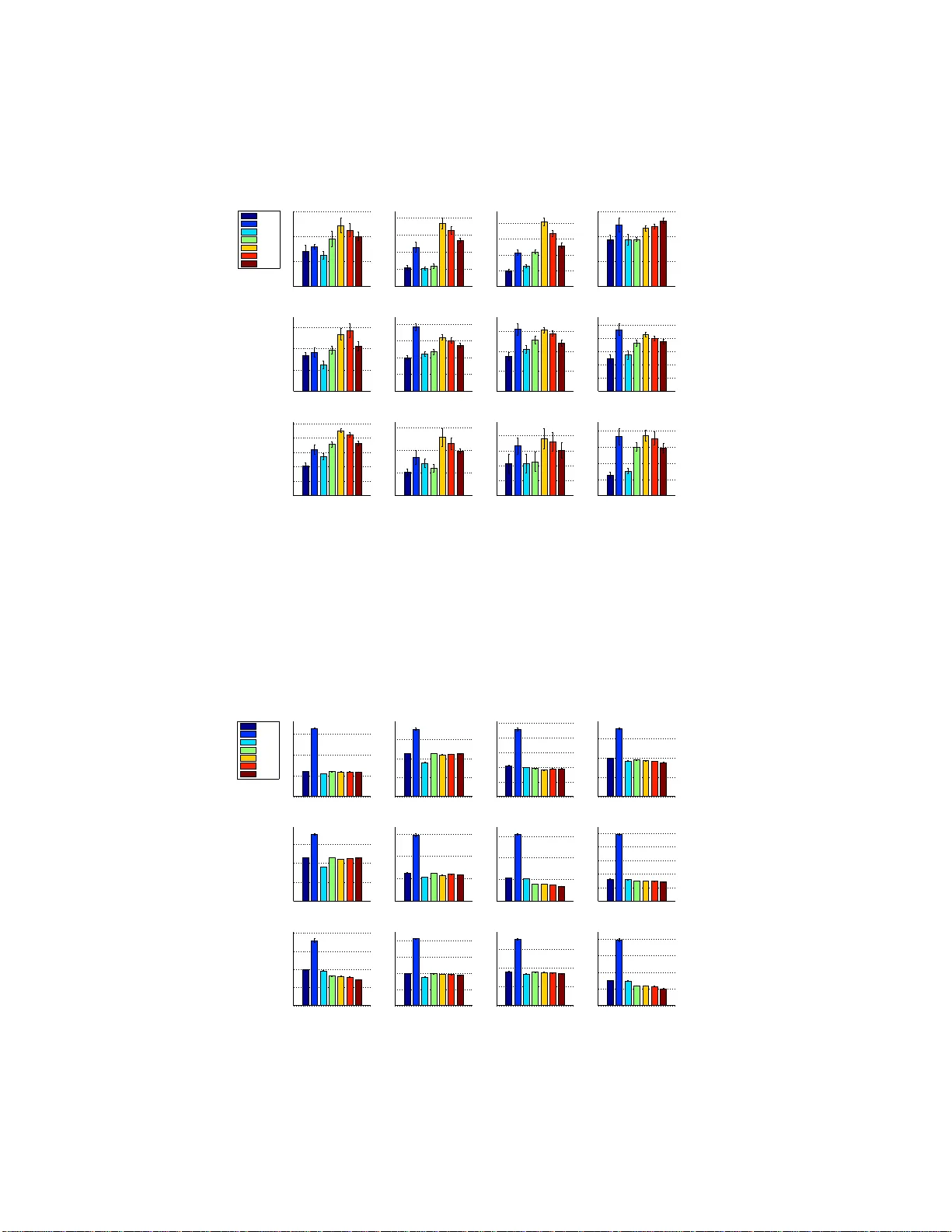
Alignmen t Based K ernel Learning with a Continuous Set of Base K er nels Arash Afkanpour Csaba Szepesv ´ ari Michael Bowling Departmen t of C omp uting Science University of Alberta Edmon ton, AB T6G 1K7 { afkanpou, szepesva,mbo wling } @ualberta .ca Abstract The success of kernel-based learning methods depend on the choice of kernel. Recently , kerne l learning metho ds h av e been pr oposed that u se data to select the most app ropriate kerne l, u sually by combining a set of base kernels. W e intro- duce a new algorithm fo r kerne l le arning th at com bines a continuo us set of ba se kernels , without the com mon step of discretizing the space of base kernels. W e demonstra te that ou r ne w method achiev es state-of-the-art performa nce across a variety of real-world datasets. Furthermo re, we explicitly demonstrate the im- portance o f combinin g the right d ictionary of kern els, wh ich is pr oblematic for methods b ased on a finite set of base kernels c hosen a priori. Our metho d is not the first approac h to work with contin uously par ameterized kernels. Howev er, we show that o ur metho d r equires substantially less computation than previous such approa ches, an d so is mor e amenable to multiple dimensional parameterizatio ns of base kernels, which we demonstrate. 1 Intr oduction A well kn own fact in machine learning is that the choice o f f eatures he avily influences th e p er- forman ce of learning methods. Similarly , the performan ce of a learning method that uses a kernel function is highly depend ent on the choice of kernel fu nction. The idea of kernel learning is to use data to select the most appro priate kernel functio n for the learn ing task. In this pape r we co nsider kern el learning in the con text of super vised learning . In particular, we consider the pr oblem o f lea rning positive-coefficient linear combin ations of base kern els, where the base kernels belon g to a param eterized family of kernels, ( κ σ ) σ ∈ Σ . Here Σ is a “co ntinuou s” parameter space, i.e., som e subset o f a Euclidean spa ce. A prime example (and extrem ely pop ular choice) is when κ σ is a Gaussian kern el, where σ can be a single common ban dwidth or a vecto r of bandwidths, one per coordin ate. One approach then is to discretize the par ameter space Σ and then find an ap propr iate non- negativ e linear combin ation of the resulting set o f base kernels, N = { κ σ 1 , . . . , κ σ p } . The advantage of th is appro ach is that onc e the set N is fixed, any of the many efficient metho ds av ailable in th e literature can be used to find the c oefficients for combinin g the b ase kernels in N (see the papers by Lanckriet et al. 2004; Sonnenburg et al. 2 006; Rakotomamonjy et al. 2008; Cortes et al. 2009a; K loft et al. 20 11 and th e ref erences therein). One potential d rawback o f this appr oach is that it requires an appro priate, a priori choic e of N . T his might be pro blematic, e.g., if Σ is conta ined in a E uclidean space o f m oderate, or large dim ension (say , a d imension over 20) since the number of base kernels, p , grows exponentially with dimensionality even for mod erate discretization accuracies. Furthermo re, in depend ent o f the d imensionality of th e parameter sp ace, the n eed to choo se the set N ind ependen tly of the d ata is at best in conv enient and selecting an 1 approp riate resolution might b e far from trivial. In this paper w e explor e an alternative me thod which av oids the need for discretizing the space Σ . W e are no t the fir st to realize that discretizin g a c ontinuo us parameter space mig ht be tro ublesome : The method of Argyrio u et al. (20 05, 2006) can also work with con tinuously par ameterized spaces of kernels. T he main iss ue with this method , howe ver , is that it may get stuck in local optima since it is b ased on alternating minim ization and th e ob jectiv e function is no t jointly co n vex. Nevertheless, empirically , in the initial publications of Argyriou et al. (2005, 200 6) this method was foun d to ha ve excellent and robust p erform ance, sho wing that despite the p otential difficulties, the idea of av oiding discretizations might have some traction. Our new meth od is similar to that of Argyriou et al. (2005, 2006), in that it is still based on local search. Howev er, our lo cal searc h is used with in a boosting , or more pr ecisely , forward-stag ewis e additive modeling (FSAM) proce dure, a method that is known to be quite robust to h ow its “greed y step” is implemen ted (Hastie et al., 2001, Sectio n 1 0.3). Thu s, we expect to suffer minim ally f rom issues related to local minima. A second difference to Argyriou et al. ( 2005, 20 06) is that our m ethod belongs to the gro up of two-stage kernel learnin g m ethods. The decision to u se a two-stage kernel learning app roach was mo tiv ated b y th e recen t success of the two-stage metho d of Cortes e t al. (2010). I n fact, our k ernel learning m ethod uses the c entered kernel alignmen t m etric of C ortes et al. (2010) (derived f rom the uncentered alignment metric of Cristianini et al. (2 002)) in its first stage as th e objectiv e fun ction of the FSAM pro cedure, while in the secon d stage a standard supe rvised learning techniqu e is used. The technical dif ficulty of implementing FSAM is that one needs to compute the functional gradient of the ch osen ob jectiv e fun ction. W e sho w th at in o ur case this pro blem is equivalent to solving an optimization problem ov er σ ∈ Σ with an ob jectiv e function that is a lin ear function o f the Gr am matrix deri ved fro m th e kernel κ σ . Because of the nonlinear d ependen ce of this matrix on σ , this is the step wher e we need to resort to local optim ization: this optimizatio n problem is in general non-co n vex. Howe ver , a s we shall d emonstrate empirically , even if we u se local so lvers to solve this o ptimization step, the algorithm still shows an overall excellent perf ormanc e as compar ed to other state-o f-the-ar t methods. This is no t completely un expected: One of the key ideas un derlying boosting is th at it is d esigned to be robust e ven when the ind i vidu al “g reedy” steps are imperfect (cf., Chapter 12, B ¨ uhlmann and van de Geer 2 011). Gi ven the new kernel to be added to the existing dictionary , we gi ve a computa tionally efficient, closed-form expr ession that can be used to determine the coefficient on the new kernel to be added to the pre vious kernels. The emp irical perf ormanc e of o ur pr oposed method is explor ed in a series of experim ents. Our experiments serve multiple purposes. Firstly , we explore the poten tial adv antages, as well as limita- tions o f the proposed techniq ue. In par ticular, we demo nstrate that the proce dure is indeed reliable (despite the potential difficulty of implem enting the greed y step) and that it can be s uccessfu lly used ev en when Σ is a subset of a multi-dimension al space. Second ly , we demonstrate that in some cases, kernel learnin g can have a very large imp rovement over simpler alter nativ es, such as com bining some fixed dictio nary of kernels with un iform weights. Whether this is true is an important issue that is given weigh t by the fact that just r ecently it beca me a subject o f dispute ( Cortes, 2 009). Fi- nally , we com pare the p erform ance o f our m ethod, both from the pe rspective of its generalizatio n capability and c omputatio nal cost, to its natural, state-of-th e-art altern ativ es, such as the two-stage method of Cortes et al. (201 0) and the algo rithm of Argyr iou et al. (200 5 , 2006). For this, we co m- pared our meth od on datasets used in p revious kernel-learnin g work. T o give further weight to our results, we co mpare on more datasets than any o f th e p revious pap ers that prop osed new kerne l learning method s. Our experiments demonstrate that our new method is competitive in terms of its generalization per - formance, while its compu tational cost is sign ificantly less than tha t of its competitors that enjoy similarly go od generalization performa nce as our meth od . In add ition, ou r experiments also re- vealed an interesting n ovel insight into the b ehavior of two-stage m ethods: we no ticed that two- stage methods can “overfit” the perform ance metric of the first stage. In s ome prob lem we observed that our method could find kern els th at ga ve rise to better (test-set) per forman ce on the first-stage metric, while the m ethod’ s overall perf ormanc e degrades when compar ed to using kern el combina- tions whose per forman ce on the fir st m etric is worse. Th e explan ation of this is that metric of the first stage is a surrog ate perfor mance measure and thus just like in the case of cho osing a surr o- gate l oss in classification, better perfo rmance according to this surrog ate metric does not necessarily 2 transfer in to better perfo rmance in the primary metric as there is no mon otonicity relation between these two metrics. W e also show that with proper capacity control, the problem of overfitting the surrogate metr ic can be overcome. Finally , our experiments show a clear advantage to using kern el learning method s as opposed to com bining kernels with a unifor m weight, althou gh it seems that the advantage mainly comes from the ability of our method to discover the right set of kernels. This conclusion is strengthened by the fact that the closest com petitor to our method w as found to be the method of Argyrio u et al. (200 6) th at also searches the con tinuou s param eter spa ce, av oiding dis- cretizations. Our conclusion is that it seems that the choice of the base dictionary is more impo rtant than how the dictionary elements are combined and that the a priori choice of th is diction ary may not be tr ivial. This is certainly tru e already when th e number of par ameters is mod erate. Moreover, when the nu mber of p arameters is larger , simple discretizatio n metho ds are inf easible, where as our method can still produ ce meanin gful dictionaries. 2 The New Method The purpo se of this section is to describe our new metho d. Let us start with the introd uction of the problem setting and the n otation. W e consider binary classification p roblems, wh ere the data D = (( X 1 , Y 1 ) , . . . , ( X n , Y n )) is a sequenc e of indepe ndent, identically distributed ra ndom variables, with ( X i , Y i ) ∈ R d × {− 1 , +1 } . For con venience, we introduce two other pairs of random v ariables ( X, Y ) , ( X ′ , Y ′ ) , which ar e a lso in depend ent of eac h o ther an d they share the same distribution with ( X i , Y i ) . T he g oal o f classifier learn ing is to fin d a predicto r , g : R d → {− 1 , +1 } such th at the predictor’ s risk, L ( g ) = P ( g ( X ) 6 = Y ) , is close to the Bayes-risk, inf g L ( g ) . W e will consider a two-stage method, as n oted in the intro duction. The fir st stage of ou r method will pick some kernel k : R d × R d → R from some set of kerne ls K based on D , which is then used in the seco nd stage, using the same data D to find a good predictor . 1 Consider a parame tric family of base kern els, ( κ σ ) σ ∈ Σ . The kernels considered b y o ur method belong to the set K = ( r X i =1 µ i κ σ i : r ∈ N , µ i ≥ 0 , σ i ∈ Σ , i = 1 , . . . , r ) , i.e., we allow no n-negative linear combinations of a finite nu mber of b ase kernels. For exam- ple, the base kernel cou ld be a Gau ssian kernel, where σ > 0 is its b andwidth : κ σ ( x, x ′ ) = exp( −k x − x ′ k 2 /σ 2 ) , wh ere x, x ′ ∈ R d . Howe ver , on e could also have a separate ban dwidth for each coordina te. The “ideal” kernel unde rlying the common distribution of the data is k ∗ ( x, x ′ ) = E [ Y Y ′ | X = x, X ′ = x ′ ] . Our new meth od attempts to find a kernel k ∈ K whic h is maximally aligned to this id eal kernel, where, following Cortes et al. (2010), the alignment between tw o kernels k , ˜ k is measured by the center ed alignmen t metric , 2 A c ( k , ˜ k ) def = h k c , ˜ k c i k k c kk ˜ k c k , where k c is the kernel underlying k cente red in the feature space (similarly fo r ˜ k c ), h k, ˜ k i = E h k ( X , X ′ ) ˜ k ( X , X ′ ) i and k k k 2 = h k , k i . A kernel k cen tered in the feature space, by defin ition, is the unique kernel k c , such that for any x , x ′ , k c ( x, x ′ ) = h Φ( x ) − E [Φ( X )] , Φ( x ′ ) − E [Φ( X )] i , where Φ is a feature map unde rlying k . By con sidering cen tered kernels k c , ˜ k c in th e alignm ent metric, one im plicitly matches the mean respo nses E [ k ( X , X ′ )] , E [ ˜ k ( X , X ′ )] before consider ing the alignment betwee n the kernels (thus, c entering depends on the d istribution of X ). An alterna- ti ve way of stating this is that centering cance ls mismatches of the mean responses between the tw o kernels. When o ne of the kernels is the ideal kernel, centered alignment ef fectively standardizes the alignment by cancelling the effect of im balanced class distrib ution s. For furthe r discu ssion of th e virtues of centered alignmen t, see the pape r by Cortes et al. (2010). 1 One could consider splitting the data, but we see no adv antage to doing so. Also , the methods for the second stage are not a focus of this work and the particular methods used in the e xperiments are described later . 2 Note that the word metric is used in its e veryda y sense and not in its mathematical sense. 3 Algorithm 1 Forward stagewise additive m odeling f or kernel lear ning with a co ntinuou sly parametrize d set of kernels. For the defin itions of f , F , F ′ and K : K → R n × n , see the text. 1: Inputs: data D , kern el initialization parameter ε , th e numb er of iterations T , tolera nce θ , max- imum stepsize η max > 0 . 2: K 0 ← εI n . 3: for t = 1 to T do 4: P ← F ′ ( K t − 1 ) 5: P ← C n P C n 6: σ ∗ = a rg max σ ∈ Σ h P, K ( κ σ ) i F 7: K ′ = C n K ( κ σ ∗ ) C n 8: η ∗ = a rg max 0 ≤ η ≤ η max F ( K t − 1 + η K ′ ) 9: K t ← K t − 1 + η ∗ K ′ 10: if F ( K t ) ≤ F ( K t − 1 ) + θ t hen terminate 11: end for Since the common distribution un derlying the data is unknown, one resorts to empirical approxima- tions to alignmen t and center ing, resulting in the empirical alignment metric, A c ( K, ˜ K ) = h K c , ˜ K c i F k K c k F k ˜ K c k F , where, K = ( k ( X i , X j )) 1 ≤ i,j ≤ n , an d ˜ K = ( ˜ k ( X i , X j )) 1 ≤ i,j ≤ n are the kern el matrices underlying k and ˜ k , and for a kernel matrix, K , K c = C n K C n , wh ere C n is the so-c alled centering matrix defined by C n = I n × n − 11 ⊤ /n , I n × n being the n × n iden tity matrix and 1 = (1 , . . . , 1) ⊤ ∈ R n . The empirical counterpar t of maximizing A c ( k , k ∗ ) is to maximize A c ( K, ˆ K ∗ ) , where ˆ K ∗ def = YY T , and Y = ( Y 1 , . . . , Y n ) ⊤ collects the responses into an n - dimension al v ector . Here, K is the kernel matrix derived from a kernel k ∈ K . T o make this conn ection clear , we will write K = K ( k ) . Define f : K → R by f ( k ) = A c ( K ( k ) , ˆ K ∗ ) . T o find an approx imate maximizer of f , we propose a steepest ascent approach to forwar d s tagewise additive modelin g (FSAM). FSAM (Hastie et al., 20 01) is an iterative method for optim izing an objective function b y sequentially addin g ne w basis fun ctions without chang ing the parameters and coefficients of the p reviously add ed basis fun ctions. In th e steepest ascent a pproac h, in iteration t , we search for the base kernel in ( κ σ ) defining the direction in which the growth rate of f is the largest, locally in a small neighborh ood of the previous candida te k t − 1 : σ ∗ t = a rg max σ ∈ Σ lim ε → 0 f ( k t − 1 + ε κ σ ) − f ( k t − 1 ) ε . (1) Once σ ∗ t is found, the algorithm finds the coefficient 0 ≤ η t ≤ η max 3 such that f ( k t − 1 + η t κ σ ∗ t ) is maxim ized and the candidate is u pdated using k t = k t − 1 + η t κ σ ∗ t . The process stops when the objective function f ceases to increase by an amoun t larger th an θ > 0 , or when the number of iterations becomes larger then a predetermined l imit T , whichever happens earlier . Proposition 1. The value of σ ∗ t can be obtaine d by σ ∗ t = arg max σ ∈ Σ  K ( κ σ ) , F ′ ( ( K ( k t − 1 )) c )  F , (2) wher e for a kernel matrix K , F ′ ( K ) = ˆ K ∗ c − k K k − 2 F h K, ˆ K ∗ c i F K k K k F k ˆ K ∗ c k F . (3) The p roof can be found in the supplemen tary mater ial. The crux of th e pr oposition is th at the directional deriv ative in (1) can be calculated and gi ves the expression maximized in (2). 3 In all our experiments we use the arbitrary v alue η max = 1 . Note t hat the v alue of η max , together with the limit T acts as a regularizer . Howe ver , in our experimen ts, the procedure al ways stops b efore the limit T on the number of iterations is reached. 4 T able 1: List of the kernel learning metho ds evaluated in the experiments. The ke y to the naming of the methods is as follows: CA stands for “continuou s a lignment” m aximization , CR stands for “continuo us risk” minimization, D A stands f or “discrete alignment”, D1, D2, DU s hou ld b e obvious. Abbr . Method CA Our new method CR From Argyriou et al. (2005) D A From C ortes et al. (2 010) D1 ℓ 1 -norm MKL (Kloft et al., 2011) D2 ℓ 2 -norm MKL (Kloft et al., 2011) DU Uniform weights over kernels In general, the op timization pr oblem (2 ) is n ot convex and the cost of obtain ing a (good ap proxim ate) solution is hard to pred ict. Evid ence that, at le ast in some cases, th e f unction to be optimized is not ill-behaved is presented in Section B.1 of the sup plementar y material. In our experiments, an approx imate s olutio n to (2) is fou nd using numerical metho ds. 4 As a final remark to this issue, note that, as is usual in boosting, finding the global optimizer in (2) might not be necessary for achieving good statistical perform ance. The othe r paramete r , η t , ho wever , is easy to find, since the und erlying optimization pr oblem has a closed form solution: Proposition 2. The value of η t is given by η t = arg max η ∈ { 0 , η ∗ ,η max } f ( k t − 1 + η κ σ ∗ t ) , wher e η ∗ = max(0 , ( ad − bc ) / ( bd − ae )) if bd − ae 6 = 0 a nd η ∗ = 0 o therwise, a = h K , ˆ K ∗ c i F , b = h K ′ , ˆ K ∗ c i F , c = h K , K i F , d = h K, K ′ i F , e = h K ′ , K ′ i F and K = ( K ( k t − 1 )) c , K ′ = ( K ( κ σ ∗ t )) c . The pseudo code of the full algo rithm is presented in Algo rithm 1. The algorithm needs the d ata, the n umber of iterations ( T ) and a toleran ce ( θ ) parame ter , in ad dition to a p arameter ε used in the initialization phase and η max . The parame ter ε is used in the in itialization step to av oid divi- sion by zero, and its v alue has little effect on the p erform ance. Note tha t the cost of comp uting a kernel-matrix , or the inn er product of two such matrices is O ( n 2 ) . Therefor e, the co mplexity of the algorithm (with a na i ve im plementation ) is at lea st quad ratic in the number of samples. The ac tual cost will be strongly influen ced by ho w many of these kernel-matrix evaluations (o r inn er pro duct computatio ns) are needed in (2). In the lack of a b etter u nderstan ding of this, we include actual runnin g times in the experimen ts, which gi ve a rough indicatio n o f the com putational limits of the proced ure. 3 Experimental Evaluation In this section we compar e o ur kernel learn ing meth od with several kernel le arning methods o n synthetic and real data; see T able 1 fo r the list o f meth ods. Our m ethod is labeled CA f or Con- tinuous Alignment- based kernel lear ning. In all of the experiments, we use the following values with CA: T = 50 , ε = 10 − 10 , and θ = 10 − 3 . The fir st two metho ds, i.e . our algorithm , and CR (Argy riou et al., 2 005), are able to p ick kernel paramete rs from a con tinuous set, while the rest of the algorithms work with a finite number of base kernels. In Section 3.1 we u se synth etic d ata to illu strate the po tential advantage of method s that work with a con tinuou sly parameterized set of kernels and th e imp ortance of combinin g multiple kerne ls. W e also illustrate in a toy example that multi-d imensional kernel param eter search can im prove perfor- mance. The se are followed by the ev aluation of the above listed metho ds on se veral real datasets in Section 3.2. 3.1 Synthetic Data The purp ose of these experim ents is mainly to provide empiric al proof for the follo wing hypo theses: (H1) Th e combin ation of multiple kernels can lead to imp roved perfor mance as compared to what 4 In particular , we use the fmincon fu nction of Matlab, wit h the interior -point algorithm option. 5 can b e ach iev ed with a sing le kerne l, even wh en in theory a single kernel f rom the family suffices to get a co nsistent classifier . (H2 ) The methods that searc h the continu ously parameterized families are ab le to find the “key” kernels and their com bination. (H3) Ou r method can even search multi- dimensiona l parameter spaces, wh ich in some cases is crucial for good performan ce. T o illustrate (H1) an d (H2) we have designed the following problem: the in puts are g enerated fro m the u niform distrib ution ov er the interval [ − 1 0 , 10] . The lab el of each d ata po int is determined b y the function y ( x ) = sign ( f ( x )) , where f ( x ) = sin( √ 2 x ) + sin( √ 12 x ) + sin( √ 60 x ) . T raining and validation sets in clude 50 0 data points each, while the test set includes 1 000 instances. Figure 1(a) shows the fun ctions f ( blue curve) and y (r ed dots). For this experiment we use Dirichlet kernels of degree one, 5 parameteriz ed with a freq uency parameter σ : κ σ ( x, x ′ ) = 1 + 2 cos( σ k x − x ′ k ) . In o rder to in vestigate (H1), we tr ained classifiers with a sin gle fr equency kernel fro m the set √ 2 , √ 12 , and √ 60 (which we thought were good guesses of the single best frequencie s). The trained classifiers achieved misclassification error rates of 2 6 . 1% , 2 6 . 8% , a nd 28 . 6% , respectively . Clas- sifiers trained with a pair o f frequencies, i.e. { √ 2 , √ 12 } , { √ 2 , √ 60 } , and { √ 12 , √ 60 } achieved error rates o f 16 . 4% , 2 0 . 0% , an d 21 . 3% , r espectively (the kernels were comb ined using un iform weights). Fin ally , a classifier that was train ed with all three f requenc ies achieved a n error rate o f 2 . 3% . Let us now turn to (H2). As sho wn in Figu re 1 (b), the CA and CR methods both ac hieved a mis- classification er ror close to what was seen when the three be st freq uencies were used, showing that they are indeed effecti ve. 6 Furthermo re, Figure 1(c) shows that the discovered frequencies are close to the frequencies used to generate th e data. For the sake of illustration, we also tested the meth- ods which req uire the discretization of th e parameter space. W e choose ten Dirich let kernels with σ ∈ { 0 , 1 , . . . , 9 } , covering the range o f f requen cies d efining f . As can be seen from Figu re 1(b ) in this examp le the chosen discre tization accuracy is insuf ficient. Althou gh it would be easy to in- crease the discretizatio n accuracy to improve the results of these method s, 7 the point is that if a high resolution is need ed in a sing le-dimension al problem, then these metho ds ar e likely to face serious difficulties in prob lems when the space of kerne ls is mo re complex (e.g., the par ameterization is multidimen sional). Nevertheless, we are not sug gesting that the m ethods which re quire discretiza- tion are universally infer ior , but m erely wish to point out th at an “appropriate discrete kern el set” might not alw ays be available. T o illustrate (H3) we designed a seco nd set o f problems: The instances for the positive (n egati ve) class ar e genera ted fr om a d = 50 - dimension al Gaussian distrib ution with cov ariance matrix C = I d × d and mean µ 1 = ρ θ k θ k (respectively , µ 2 = − µ 1 for the negative class). Here ρ = 1 . 75 . The vector θ ∈ [0 , 1] d determines the relev ance of each feature in the classification task, e.g. θ i = 0 implies that the distributions of th e two classes ha ve zero means in the i th feature, wh ich render s this feature irrelev ant. The v alue of each comp onent of v ector θ is calculate d as θ i = ( i/d ) γ , where γ is a constant that determines the relativ e imp ortance of the elements of θ . W e g enerate seven datasets with γ ∈ { 0 , 1 , 2 , 5 , 1 0 , 20 , 4 0 } . For each value of γ , the train ing set consists of 50 data points (th e p rior distribution for the two classes is u niform ). The test er ror values are measur ed on a test set with 100 0 instanc es. W e repeated each experiment 10 tim es and r eport the average misclassification error and alignment measured over the test set along with the run ning time. W e test two version s of our method : o ne that uses a family of Gaussian kernels with a com - mon b andwidth (d enoted by CA-1D) , an d ano ther on e (d enoted by CA-nD) that searches in the space ( κ σ ) σ ∈ (0 , ∞ ) 50 , where e ach coordinate has a separate bandwid th par ameter, κ σ ( x, x ′ ) = exp( − P d i =1 ( x i − x ′ i ) 2 /σ 2 i ) . Since the training s et is small, one can easily overfit while optimizing the alignment. Hence, we modif y the alg orithm to shrink the values of the bandwidth para meters to 5 W e r epeated the experimen ts using Gaussian kernels with nearly identical results. 6 In all of the experimen ts in this paper , the classifiers for the two-stage method s were trained using the soft margin S VM method, where the reg ularization coefficient of SVM was chosen by cross-v alidation from 10 {− 5 , − 4 . 5 ,..., 4 . 5 , 5 } . 7 Further experimentation found that a discretization belo w 0 . 1 is necessary in this example. 6 ! !" ! # " # !" ! $ ! % ! ! " ! % $ &'( ! "! #! $! %! &'()*+((',')+-'./0122.2345 0 0 365 78 79 :8 :" :# :; ! < "! ! !=" !=# !=$ !=% !=< >12/1*0,21?@1/)A >12/1*0B1'CD- 3)5 Figure 1: (a): Th e functio n f ( x ) = sin( √ 2 x ) + sin( √ 12 x ) + sin( √ 60 x ) used for generatin g synthetic data, a long with sign ( f ) . (b): Misclassification p ercentages o btained b y each algorithm. (c): The kernel frequencies found by the CA method. their common a verage value by modifying (2 ): σ ∗ t = a rg min σ ∈ Σ −  K ( κ σ ) , F ′ ( ( K ( k t − 1 )) c )  F + λ k σ − ¯ σ k 2 2 , (4) where, ¯ σ = 1 r P r i =1 σ i and λ is a regularization par ameter . W e also include resu lts ob tained for finite kernel learn ing methods. For these methods, we generate 5 0 Gaussian kern els with band widths σ ∈ mg { 0 ,..., 49 } , where m = 1 0 − 3 , and g ≈ 1 . 33 . There fore, the bandwidth range constitutes a geometric sequ ence from 10 − 3 to 1 0 3 . Furthe r details o f the experim ental setup can be fou nd in Section B.2 of the supplementar y mater ial. Figure 2 shows the results. Recall that the larger the value of γ , the larger the nu mber of nearly irrelev ant features. Since meth ods which search only a one- dimensiona l space cann ot d ifferentiate between re lev ant and irrelevant features, their misclassification rate increases with γ . Only CA-nD is a ble to cope with this situatio n and ev en im prove its per forman ce. W e observed that with out regularization, thoug h, CA-nD drastically overfits (for small values of γ ). W e also sho w the running times of the method s to giv e the reader an id ea about the scalability of the method s. Th e running time of CA-n D is larger than CA-1D b oth because of th e use of cross-validation to tune λ and because of the increased cost of the multid imensional searc h. Althoug h the large running time might be a problem , for some p roblems, CA-nD migh t be the o nly m ethod to deliver g ood pe rforma nce amongst the methods studied. 8 3.2 Real Data W e evaluate the metho ds listed in T ab le 1 on se veral binar y c lassification tasks fr om MNIST and the UCI Letter re cognition dataset, along with several other da tasets from the UCI machine learning repository (Frank and Asuncion, 2010) and Delve datasets (see, http://www.c s.toronto.e du/ ˜ delve/data/d atasets.htm l ). 8 W e have not att empted to run a multi-dimensional version of the CR method, since already the one- dimensional version of this method is at least one orde r of magnitude slower than ou r CA-1D method. 7 0 1 2 5 10 20 40 0 0.1 0.2 0.3 0.4 0.5 γ misclassification error 0 1 2 5 10 20 40 10 0 10 1 10 2 10 3 10 4 γ running time (sec.) CA−1D CA−nD CR DA D1 D2 DU Figure 2: Performan ce and running time of various methods for a 50 -dim ensional synthetic problem as a fun ction of the relev ance parameter γ . Note that the number of irrelevant featur es in creases with γ . For details of the exp eriments, see the text. T able 2: Median rank and runn ing time (sec.) of kernel learning methods obtained in experiments. CA-1D CA-nD CR D A D1 D2 DU Rank MNIST 1 N/A 2 4.5 4.5 5 4 Letter 1 4.5 2 3.5 7 6 5 11 datasets 3 2 3 3 4 6 6 T ime MNIST 12 ± 1 N/A 3 77 ± 5 6 31 ± 1 57 ± 6 58 ± 3 10 ± 1 Letter 9 ± 1 1986 ± 24 7 590 ± 21 11 ± 1 21 ± 1 22 ± 1 5 ± 1 MNIST . In the first experim ent, following Argyriou et al. (20 05), we choose 8 handwritten d igit recogn ition tasks of various d ifficulty from the MNI ST dataset (LeCun and Cortes, 20 10). Th is dataset con sists of 28 × 28 images with pixel values ranging be tween 0 and 2 55 . In these experim ents, we used Gaussian kern els with parameter σ : G σ ( x, x ′ ) = exp( −k x − x ′ k 2 /σ 2 ) . Du e to th e large number of attrib utes (784) in the MNIST dataset, we only e valuate the 1-dimension al version of our method. F or the algorithms that work with a finite kernel set, we pick 20 kernels with the value of σ picked f rom an equidistant d iscretization of interval [5 00 , 50 0 00] . In each experiment, the tr aining and validation sets con sist of 500 and 1 000 data p oints, while the test set has 2 000 data points. W e repeated each experiment 10 times. Due to the lack of space, the test-set er ror plots fo r all of the pro blems can be found in the supp lementary material ( see Section B.3 ). In order to g iv e an overall imp ression of the algorith ms’ performan ce, we ranked them based on the results obtained in the ab ove exper iment. T ab le 2 rep orts th e median ra nks of the method s for the experiment just described. Overall, meth ods that choose σ from a con tinuous set outperfor med their finite cou nterpar ts. Th is suggests again that for the finite kernel learning metho ds the ran ge of σ and the discretization of this range is important to the accuracy of the resulting classi fier . UCI Letter Recognition. In another experim ent, w e ev aluated these m ethods on 12 binary clas- sification tasks fro m the UCI Letter rec ognition dataset. This dataset includes 200 00 data po ints of the 26 capital letter s in the En glish alphabet. F or each binary classification task, the training and v al- idation sets include 300 and 200 data points, respectively . T he misclassification erro rs are measured over 100 0 test po ints. As with MNIST , we used Gaussian kernels. Howe ver , in this experimen t, we ran our method with both 1-dimension al and n -dim ensional search procedures. T he rest of the meth- ods lear n a single parameter and the finite kernel learning metho ds were provided with 20 kernels with σ ’ s chosen from the interval [1 , 200] in an equidistant manner . The plo ts o f misclassification error and alignm ent are a vailable in the supplemen tary material (see Section B.3). W e report the me- dian ran k of each method in T able 2. While the 1-dimension al version of ou r method ou tperfor ms 8 the r est o f th e method s, the classifier built o n th e kern el fou nd by the mu lti-dimension al version of our method did not p erform well. W e examined the value of alignm ent between the lea rned kern el and the target label kern el on the test set achie ved by each meth od. The results are available in the supplemen tary material (see Section B.3). The multid imensional version of our metho d achiev ed the high est value of alignmen t in every task in this experiment. Hig her value of alignme nt between the lear ned kernel a nd the ideal kernel d oes no t nec essarily translate into high er value of acc uracy of th e classifier . Aside from this o bservation, the same trends observed in the MNIST data can be seen here. The continuo us kernel learning methods (CA-1D and CR) ou tperfo rm th e finite kernel learning method s. Miscellaneous data sets. In the last experime nt we ev aluate all method s on 11 datasets cho sen from the UCI machine learnin g repository and Delv e datasets. Most of these datasets were used p re- viously to ev aluate kernel learning algorithms (Lanckriet et al., 20 04; Cortes et al., 2009a,b, 2010; Rakotomamon jy et al., 2008). T he specification of each dataset and the perfo rmance o f each method are available in the supp lementary mater ial (see Section B.3). The median rank o f each method is shown in T able 2. Contrary to the Letter experimen t, in th is case the multi-dim ensional version of our method outperfo rms t he rest of the meth ods. Running Times. W e measured the time req uired for each run and each kernel learning method in the MNIST an d th e UCI Letter experiments. In each case we too k the average of th e runn ing time of e ach method over a ll task s. T he average r equired time alon g with the standard er ror values are shown in T able 2. Amo ng all methods, the DU method is fast est, which is e xpe cted, as it requires no additional time to comp ute kernel weights. The CA-1D is the fastest among the rest of the metho ds. In these exper iments our method con verges in less than 10 iterations ( kernels). The gener al trend is that one-stage kernel learning m ethods, i.e., D1 , D2, and CR, are slower than tw o-stage metho ds, CA and D A. Among all method s, the other continuou s kerne l learning metho d, CR, is slo west, since (1) it is a one-stag e algo rithm and (2) it usually requires more iterations (around 50 ) to con verge. W e also examin ed the DC-Programm ing v ersion of the CR m ethod Argyriou et al. (200 6 ). While it is faster than the original gradient-b ased approach (roug hly three ti mes fas ter), it is still significantly slower than the rest o f the methods in our experiments. 4 Conclusion and Futur e W ork W e presented a novel metho d f or kernel learn ing. This method a ddresses th e problem of lear ning a kern el in th e positive linear span o f some continuo usly parameterized kernel family . The algo - rithm implements a steepest ascent ap proach to fo rward stagewise add iti ve m odeling to max imize an empirical centered co rrelation measure b etween the kernel and the empirical approx imation to the ideal response-kern el. The method was sho wn to perfor m well in a series o f experiments, both with synthetic and real-d ata. W e showed that in single-dimensional kernel parameter search, our method outperf orms standard multiple kernel learn ing meth ods with out the n eed to d iscretizing the param- eter space. While the method of Argyr iou et al. (2 005) also benefits from search ing in a con tinuou s space, it was seen to require sign ificantly mo re comp utation time co mpared to our m ethod. W e also showed that o ur meth od can successfully de al with h igh-dim ensional kernel parameter spac es, which, at least in our experiments, the method of Argyriou et al. (20 05, 2006) had problems with. The main lesson of our experiments is that the m ethods that start by d iscretizing the kernel space without using the data migh t lose the po tential to achieve good p erforma nce befor e any lear ning happen s. W e think that cur rently ou r metho d is the mo st efficient metho d to design data-dep endent dictio- naries that provide competitive performan ce. It r emains an interesting p roblem to be explo red in the future whether there exist method s that are provably efficient and yet their perfor mance remain s competitive. Although in this work we dir ectly compared our method to fin ite-kernel method s, it is also natural to comb ine d ictionary sear ch methods (like o urs) with finite-kernel le arning methods. Howe ver , the thoro ugh in vestigation of this option remains for future work. A secon dary outcome of our experimen ts is the observation that altho ugh test-set alignme nt is gen- erally a good indica tor of g ood p redictive perform ance, a larger test-set alignment do es not neces- 9 sarily transfo rm into a smaller m isclassification error . Altho ugh th is is not co mpletely u nexpected, we think that it will be important to thoroug hly explore the implications of this observation. Refer ences Argyriou, A., Hauser , R., Micchelli, C., and Pontil, M. (2006 ). A DC-prog ramming alg orithm for kernel selection. In Pr oceedings of the 23r d interna tional conference on Machine learning , page s 41–48 . Argyriou, A., Micchelli, C., and Pontil, M. (2005 ). L earning convex comb inations of co ntinuou sly parameteriz ed basic kern els. In Pr oceed ings of the 18th Annua l Confer ence on Learnin g Theory , pages 338– 352. B ¨ uhlmann, P . and van de Geer, S. (201 1). S tatistics fo r High-Dimen sional Data: Meth ods, Theory and Application s . Spr inger . Cortes, C. (2009 ). Invited talk: Can learn ing k ernels help per forman ce? In ICML ’09 , pages 1–1. Cortes, C., Mo hri, M. , and Rostamiza deh, A. ( 2009 a). L2 regularization for learning kernels. In Pr oceedings of the 25th Confer ence on Uncertainty in Artificial Intelligence , pages 109–116. Cortes, C., Mohri, M., and Rostamizadeh, A. (2009b) . Learnin g non-linear combin ations of kernels. In Advanc es in Neural Information Pr ocessing Systems 22 , pages 396–40 4. Cortes, C., Mo hri, M., and Rostamiza deh, A. (20 10). T wo-stage learnin g kern el a lgorithms. In Pr oceedings of the 27th Internationa l Conference on Machine Learning , pages 239–24 6. Cristianini, N., Kan dola, J., Elisseeff, A., and Shawe-T aylor, J. (20 02). On kernel-target alignment. In Advanc es in Neural Information Pr ocessing Systems 15 , pages 367–37 3. MIT Press. Frank, A. and Asuncion, A. (2010) . UCI mach ine learning repository . Hastie, T ., Tibshirani, R., an d Friedm an, J. (2001). The Elemen ts o f Statistical Learning . Sprin ger Series in Statistics. Springer-V erlag New Y ork. Kloft, M., Brefe ld, U., Sonn enburg, S., an d Z ien, A. (2 011). ℓ p -norm mu ltiple kernel lear ning. Journal of Machine Learning Resear ch , 12:953–9 97. Lanckriet, G., Cristianini, N., Bar tlett, P ., Ghaoui, L., and Jordan, M. (2004). Lea rning the kernel matrix with semidefinite prog ramming . J ournal of Machine Learning Resear ch , 5:27–72. LeCun, Y . and Cortes, C. (2010 ). MNIST han dwritten digit database. Rakotomamon jy , A., Bach, F ., Canu, S., an d Gr andvalet, Y . (200 8). SimpleMKL. Journal of Machine Learning Resear ch , 9:249 1–25 21. Sonnenburg, S., R ¨ atsch, G., Sch ¨ afer, C., an d Sch ¨ olkopf , B. (200 6). Large scale multiple kerne l learning. The Journal of Machine Learning Re sear ch , 7:1531–15 65. 10 A Proofs A.1 Proof of Proposition 1 First, notice that the limit in (1) is a directional deriv ative, D κ σ f ( k t − 1 ) . By the chain rule, D κ σ f ( k t − 1 ) = h K ( κ σ ) , F ′ c ( K ( k t − 1 )) i F , where, for conv enienc e, we defined F c ( K ) = A c ( K, ˆ K ∗ ) . Define F ( K ) = h K, ˆ K ∗ c i F / ( k K k F k ˆ K ∗ c k F ) so that F c ( K ) = F ( K c ) . Some calculations gi ve that F ′ ( K ) = ˆ K ∗ c − k K k − 2 F h K, ˆ K ∗ c i F K k K k F k ˆ K ∗ c k F (which is the functio n defined in (3)). W e claim that the fo llowing holds: Lemma 3. F ′ c ( K ) = C n F ′ ( K c ) C n . Pr oof. By the defin ition of deri vati ves, as H → 0 , F ( K + H ) − F ( K ) = h F ′ ( K ) , H i F + o ( k H k ) . Also, F c ( K + H ) − F c ( K ) = h F ′ c ( K ) , H i F + o ( k H k ) . Now , F c ( K + H ) − F c ( K ) = F ( C n K C n + C n H C n ) − F ( C n K C n ) = h F ′ ( K c ) , C n H C n i F + o ( k H k ) = h C n F ′ ( K c ) C n , H i F + o ( k H k ) , where the last proper ty fo llows fr om the cyclic pr operty of trace. Theref ore, by the uniqueness of deriv ative, F ′ c ( K ) = C n F ′ ( K c ) C n . Now , notice that C n F ′ ( K c ) C n = F ′ ( K c ) . Thus, we see that the v alue of σ ∗ t can be obtained by σ ∗ t = arg max σ ∈ Σ  K ( κ σ ) , F ′ ( ( K ( k t − 1 )) c )  F , which was the statement to be proved. A.2 Proof of Proposition 2 Let g ( η ) = f ( k t − 1 + η κ σ ∗ t ) . Using the definition of f , we find that with som e constant ρ > 0 , g ( η ) = ρ a + bη ( c + 2 dη + eη 2 ) 1 / 2 . Notice that here the d enomina tor is bound ed away from zero (this fo llows fro m th e f orm of the denomin ator of f ). In p articular, e > 0 . Further, lim η →∞ g ( η ) = − lim η →−∞ g ( η ) = ρ b √ e . (5) T aking the der iv ati ve of g we fin d that g ′ ( η ) = ρ bc − a d + ( bd − ae ) η ( c + 2 dη + eη 2 ) 3 / 2 . Therefo re, g ′ has at most one root a nd g has at most one global extremum, from which th e result follows by solving for the ro ot of g ′ (if g ′ does not have a root, g is co nstant). 11 0 5000 10000 ! f( ! ) (a) odd vs. even, (1) 0 5000 10000 ! f( ! ) (b) odd vs. even, (2) 5000 10000 ! f( ! ) (c) 0 vs. 6, (1) 0 5000 10000 ! f( ! ) (d) 0 vs. 6, (2) 0 50 100 ! f( ! ) (e) B vs. E, (1) 0 50 100 ! f( ! ) (f ) B vs. E, (2) 0 50 100 ! f( ! ) (g) B vs. E, (3) 0 50 100 ! f( ! ) (h) B vs. E, (4) Figure 3: The flipped ob jectiv e function underlyin g (2 ) as a f unction of σ , the parameter of a Gaus- sian kernel in selected MNIST and UCI Letter prob lems. Ou r algorithm needs to find the minimu m of these functions (and similar ones). B Details of the numerical experiments In this section we provide further details and data for the numerical results. B.1 Non-Conv exity Iss ue As we mentio ned in Section 2 , our algorithm may need to solve a non-co n vex optim ization prob lem in each iteration to find the best kernel par ameter . Her e, we explore this pro blem n umerically , b y plotting the function to be optimized in the case o f a Gaussian kernel with a single bandwidth pa ram- eter . In particular, we plotted the objec ti ve fun ction of Equa tion 2 with its sign flipped, therefo re we are in terested in the local min ima o f fu nction h ( σ ) = −  K ( κ σ ) , F ′ ( ( K ( k t − 1 )) c )  F , see Figure 3. Th e functio n h is shown for some iter ations of some o f the tasks fro m b oth the MNI ST and th e UCI Letter experime nts. The nu mber in side paren theses in th e caption specifies the c orrespon ding iteration of the alg orithm. On these p lots, the obje cti ve function does not have m ore than 2 loca l minima. Although in some cases the fu nctions have some steep parts (at th e scales shown), their optimization does not seem very dif ficult. B.2 Details of the 50-dimensional synthetic dataset experiment The 1-dime nsional version of our alg orithm, CA-1D, and the CR method, employ Matlab’ s fmincon function with multiple restarts from t he set 10 {− 3 ,..., 5 } , to choose the kernel param eters. The multi- dimensiona l version o f o ur algor ithm, CA-n D, u ses fmincon o nly once, since in this par ticular example the search method runs on a 50 - dimension al search space, wh ich makes th e search an expensiv e operatio n. Th e starting point of the CA-nD method is a vector of equal elemen ts wh ere this element is the weighted a verage of the kernel parameters found by the CA-1D method, weighted by the coefficient of the corr espondin g kernels. The soft m argin SVM regularization parameter is tuned fr om the set 10 {− 5 , − 4 . 5 ,..., 4 . 5 , 5 } using an indepen dent v alidation set with 1000 instances. W e also tun ed the value of the regula rization pa- rameter in Eq uation ( 4) f rom 10 {− 5 ,..., 14 } using the same validation set (the b est v alue of λ is the one that achieves the highest value of alignm ent on th e validation set). W e decided to use a large v al- idation set, following essentially the practice of Kloft et al. (2011, Section 6.1), to make sure that in the experimen ts reasonab ly good regularization parameters are used, i.e., to factor out the ch oice of the r egularization parameters. This mig ht bias our r esults towards CA-nD, as co mpared to CA-1D, 12 0 1 2 5 10 20 40 0 0.1 0.2 0.3 0.4 0.5 0.6 0.7 0.8 γ alignment CA−1D CA−nD CR DA D1 D2 DU Figure 4: Alignment values in the 50 -d imensional s ynth etic dataset experiment. though similar results wer e achieved with a sma ller validation set of size 200 . As a final detail note that D1 , D2 and CR also use the validation set for choo sing the value of their regular ization factor , and togethe r with the regularizer, th e weig hts also. Hence, their r esults might also b e positively biased (thoug h we don’t think this is significant, in this case). The running times sho wn in Figur e 2 inc lude e verythin g f rom the begin ning to the end, i.e., from learning the kernels to training the final classifiers (th e extra cross-validation step is what makes CA-nD expensiv e). Figure 4 shows the (centered) align ment values fo r the learned kernels (on the test data) as a function of th e relevance p arameter γ . It can be readily seen tha t the multi-dimension al meth od has a re al- edge over the other method s when the numbe r of irrelevant featu res is large, in terms of kernel alignment. As seen on Figure 4, this edge is also tran sformed into an edg e in terms of the test-set perfor mance. No te also that the discretization is fine enough so that the alignment max imizing finite kernel learning method D A can achie ve the same alignment as the method CA-1D. B.3 Detailed results f or the real datasets 0 5 10 odd vs. even 0 0.5 1 1.5 0 vs. 6 0 0.5 1 0 vs. 9 0 0.2 0.4 0.6 0.8 1 vs. 7 0 1 2 3 4 2 vs. 3 0 0.5 1 1.5 2 2 vs. 9 0 1 2 3 4 3 vs. 8 0 0.5 1 1.5 4 vs. 7 CA CR DA D1 D2 DU Figure 5: Misclassification percentag es in different tasks of the MNIST dataset. 13 0 1 2 3 B vs. E 0 1 2 3 4 B vs. F 0 2 4 6 8 C vs. G 0 1 2 3 C vs. O 0 1 2 3 E vs. F 0 2 4 6 8 I vs. J 0 1 2 3 I vs. L 0 1 2 3 4 5 K vs. X 0 1 2 3 4 5 O vs. Q 0 1 2 3 P vs. R 0 0.5 1 1.5 2 U vs. V 0 1 2 3 4 V vs. Y CA−1D CA−nD CR DA D1 D2 DU Figure 6: Misclassification percentages in dif feren t tasks of the UCI Letter recognition dataset. 0 0.2 0.4 0.6 B vs. E 0 0.2 0.4 0.6 B vs. F 0 0.1 0.2 0.3 0.4 0.5 C vs. G 0 0.2 0.4 0.6 C vs. O 0 0.2 0.4 0.6 E vs. F 0 0.2 0.4 0.6 I vs. J 0 0.2 0.4 0.6 I vs. L 0 0.1 0.2 0.3 0.4 0.5 K vs. X 0 0.1 0.2 0.3 0.4 O vs. Q 0 0.2 0.4 0.6 0.8 P vs. R 0 0.2 0.4 0.6 U vs. V 0 0.1 0.2 0.3 0.4 V vs. Y CA−1D CA−nD CR DA D1 D2 DU Figure 7: Alignment values in different tas ks of the UCI Letter rec ognition dataset. 14 T able 3: Datasets used in the experiments Dataset # features # ins tances T raining size V alidat ion size T est size Banana 2 5300 5 00 1000 2000 Breast Cancer 9 263 52 78 133 Diabetes 8 768 153 23 0 385 German 20 1000 2 00 300 500 Heart 13 270 54 81 135 Image Segmentation 18 2086 4 00 600 100 0 Ringnorm 20 7 400 50 0 1000 2000 Sonar 60 208 41 62 105 Splice 60 2991 5 00 1000 1491 Thyro id 5 215 43 64 108 W av efor m 21 5000 5 00 1000 2000 0 5 10 banana 0 10 20 30 breast cancer 0 10 20 30 diabetes 0 10 20 30 german 0 5 10 15 20 heart 0 2 4 6 8 image 0 0.5 1 1.5 ringnorm 0 10 20 30 sonar 0 5 10 15 splice 0 2 4 6 thyroid 0 5 10 waveform CA−1D CA−nD CR DA D1 D2 DU Figure 8: Misclassification percentag es obtaine d in 11 datasets. 15