On the rank-one approximation of symmetric tensors

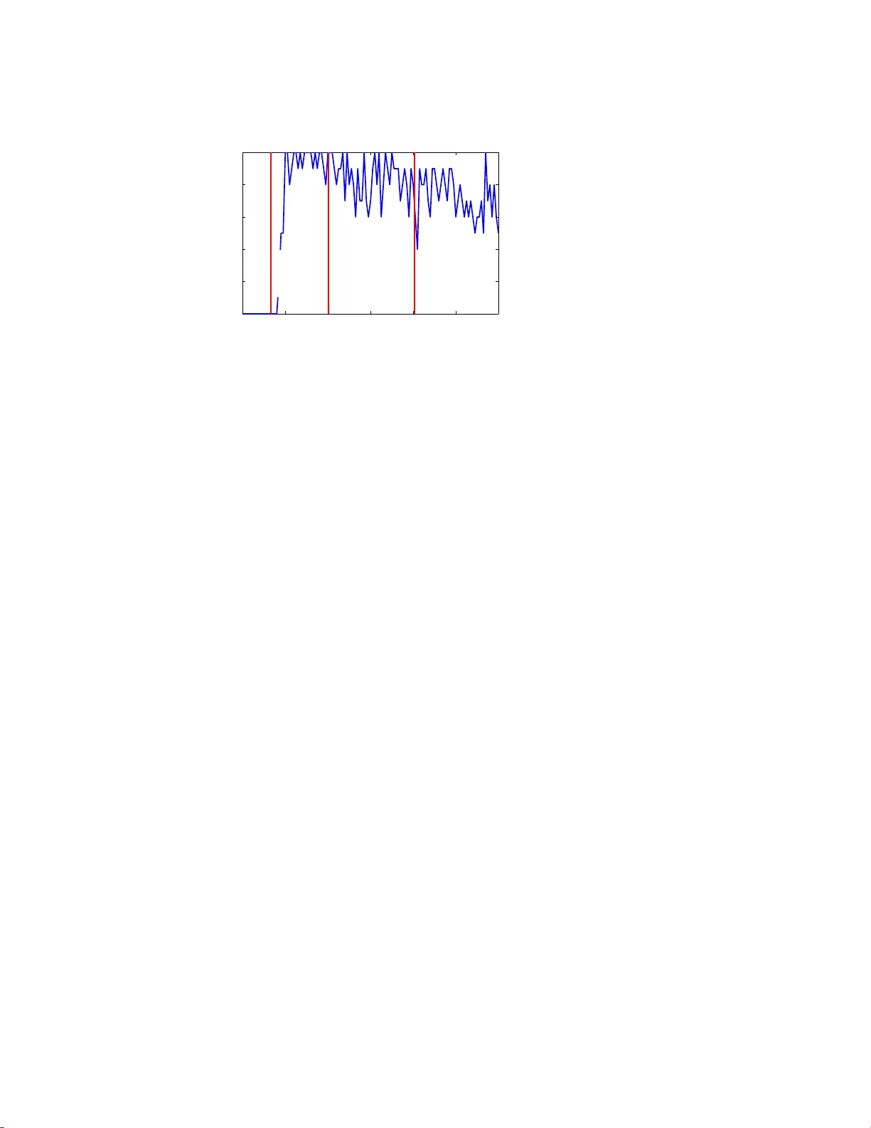
ON THE RANK-ON E APPR O XIMA TI ON O F SYMMETRIC TENSORS MICHAEL J. O’HARA ∗ Abstract. The problem of symmetric rank-one approximat ion of s ymmetric tensors is imp ortan t in Indep enden t Components Analysis, also known as Bli nd Source Separation, as well as p olynomial optimization. W e a nalyze the symmetric rank-one appro ximation problem for symmetric tensors and derive s ev er al p erturbation results. Giv en a symm etri c rank-one tensor obscured b y noise, we prov ide bounds on the accuracy of the best symmetric rank-one approximat ion for recov ering the original rank-one struc ture, and w e sho w that an y eigen vect or wi th sufficiently large eigenv alue is r elated to the rank-one structure as well. F urther, we show that for high-dimensional symmetric appro ximately-rank-one tensors, the generalized Ray leigh quotien t is mostly cl ose to zero, so the b est symmetric rank-one approximation corresp onds to a prominent global extreme v alue. W e show that eac h iteration of the Shifted Symm etri c Higher Order P o we r Method (SS-HOPM), when app lied to a rank-one symmetric tensor, mov es tow ards the principal eigenv ector f or an y input and shift parameter, under mild conditions. Finally , we explore the best ch oice of s hi ft parameter for SS- HOPM to recov er the pr incipal eigenv ector. W e show that SS-HOPM is guaran teed to con verge to an eigenv ector of an approximately rank-one eve n-mo de tensor for a wider c hoice of shift parameter than it is for a general symmetric tensor. W e also sho w that the principal eigen vecto r is a stable fixed p oint of the SS-HOPM iteration for a wide range of shift parameters; together with a n umerical experiment, these results lead to a non -obv ious recommendation for shift pa rameter for the symmetric rank-one approximation problem. Key words. symmetric rank-one appro ximation, symmetric tensors, tensors, higher-order p ow er method, shifted higher-order pow er metho d, tensor eigen v al ues, Z-eigenpa irs, l 2 eigenpairs, bli nd source s eparation, indep enden t comp onent s analysis AMS sub ject classificat ions. 15A69 1. In tro duction. The s ymmetric ra nk-one approximation of a s ymmetric tensor has at least t w o imp or tant applications. One is Indep endent Comp onents Analy s is, known in s ignals pr o cessing as Blind Sour c e Separa tion [1, 6]. Fir st, we r ecall cla ssi- cal Principa l Co mpo nent s Analysis (PCA). P CA identifi es a basis for a set o f random v ariables tha t diagonalizes the co v ar iance matrix, in o ther words a basis whe r e the random v ariables are unco r related. This is necessar y but not sufficient for indep en- dence. A stronger test for independence is to c heck whether the off-super -diagona l elements of the four-wa y cumulant tenso r, a symmetric tenso r defined from the fourth- order statistical moments, are zer o . A linear tr ansformatio n that achiev es this can b e ident ified by w r iting the tenso r as a sum of symmetric rank-one terms; o ne appro ach uses succes sive symmetric rank- one approximations [1 1]. Another imp ortant a pplication of the symmetric rank- one approximation of sy m- metric tensors is in the optimization of a general homogeneous poly no mial ov er unit length vectors, i.e. the un it spher e [8]. F or instance, the symmetric r ank-one v a riant of the “Time V a r ying Co v ar iance Approximation 2” (TV CA2) problem [10] can b e written max x : || x || =1 T X t =1 ( x T A t x ) 2 , (1.1) where { A t : t = 1 . . . T } a re a given set o f cov aria nce ma trices, and the vector norm is the 2-norm (as ar e a ll s ubsequent norms unless o ther wise indicated). The argument of ∗ Mailb ox L- 363, Lawrence Li v ermore National Lab or atory , 7000 East Ave., Livermore CA 94550 ( ohara7@ llnl.gov ). 1 2 M. J. O’HARA (1.1) is a degree -4 homogeneo us p o lynomial, a nd so as we will see the TVCA2 problem can b e repre s ented as the b est symmetric rank- one approximation of a symmetric tensor. Some things are kno wn a bo ut the symmetric r ank-one appro ximation pro ble m. The b est symmetric rank-one approximation in the F ro b e nius nor m co rresp onds to the principa l tensor eig env ector , and also the g lobal extreme v alue o f the gener alized Rayleigh q uo tient [3 , 5]. It is not clear that these facts help us s olve the symmetric rank-one approximation problem, b ecause tensor computations are gener ally notori- ously difficult. F or ins ta nce it is known [2 ] that (a symmetric) ra nk -one approximation of a genera l mo de- 3 tensor is NP- c omplete. How ever, there is an alg o rithm, the Sym- metric Shifted Higher O rder Po wer Metho d (SS-HOPM) [4], that is guar anteed to find symmetr ic tensor e ig env ector s. W e address several questions p erta ining to the rank- one appr oximation of sym- metric tensor s. In Section 3, we address the structure o f approximately-ra nk-one symmetric tensors. A symmetric rank- one tensor obs cured with no ise has a b est sym- metric r ank-one approximation that may no t b e the sa me as the or ig inal unp erturb ed tensor; how clos e is it? Is only the principa l eigenv ector r elated to the rank-one struc- ture? F or a giv en symmetric approximately-rank-one tenso r , how well-separated is the principa l eigenv alue from the spurio us eigenv alues ? In Sec tio n 4, we consider the application of SS-HOPM to a pproximately-rank-o ne symmetric tensors. How is the conv erg ence of SS-HOP M affected by the appro ximately-rank -one str ucture? When do es SS-HOP M find the principal e igenv ector ? W e employ a p erturbatio n appro ach to prove six theorems that provide ins ight all these q ue s tions. 2. Bac kground and notation. A ten s or is a multi-dimensional array of num - ber s. The n umber of mo des of the tensor , m , is the n umber of indices required to sp ecify entries; a mo de- 2 tensor is a matrix . The ra nge of p ermissible index v alues ( n 1 , . . . n m ) are the dimensions of the tensor; if all the dimensions are the same, as with symmetric tensors, w e simply write n . A symmetric tensor has en tries that are inv ariant under per m utation of indices. F o r instance, for a mo de-3 symmetric tensor A , we hav e A 123 = A 231 . In this pap er, tenso rs will b e r epresented with script capita l letters, matrices with capital letters, vectors with low er-c ase letters , and real num b ers with low erca se Gr eek letters. In teger s such a s indices, dimensio ns, etc. will also b e low erca se letter s (e.g. m, n, i . . . ). A symmet ric r ank-one tensor is the o uter pro duct of a vector with itself, which we denote using the ⊗ op e rator. F or ins tance, given the vector a , we can cons tr uct a symmetric ra nk-one tensor ( a ⊗ a ⊗ · · · a | {z } m times ) i 1 i 2 ...i m ≡ ( a ⊗ m ) i 1 i 2 ...i m = a i 1 a i 2 . . . a i m . (2.1) The r ank of a symmetric tensor A is the fewest n um ber of symmetric rank- one terms whose sum is A . Generally , the m − r pr o duct of the m -mode tenso r A with the v ector x is the r -mo de tensor defined ( A x m − r ) i 1 ...i r = n X i r +1 ,...i m =1 A i 1 ...i m x i r +1 . . . x i m . (2.2) The special case r = 0 ev alua tes to a scalar and, under the constraint || x || = 1, is called the gener alize d Ra yleigh quotient [12]. Interestingly , any degree- m homog e no us SYMMETRIC RANK- ONE APPRO X IMA TION OF SYMMETRIC TENSORS 3 po lynomial, such as (1.1), can b e written as A x m for some symmetric tensor A and indeterminate x . In a mira cle of notation, the deriv atives are conv enient ly repr esented. The g radient may b e wr itten [4] ∇A x m = m A x m − 1 , (2.3) and the Hessian may b e written [4] ∇ 2 A x m = m ( m − 1 ) A x m − 2 . (2.4) The pr oblem o f maximizing the genera lized Rayleigh quotient has the following La- grangia n: L ( x, µ ) = A x m + µ ( x T x − 1) , (2.5) where µ is the Lagrang e multiplier. Using (2.3), w e see the critical points of (2.5) satisfy the following symmetric tenso r eigenpr oblem A x m − 1 = λx . (2.6) Solutions to (2.6) with || x || = 1 are called Z eigenvalues and eigenve ctors [7] to distinguish (2.6) from other tensor eigenv ecto r problems, but here we will simply call them eigenv ecto r s and eigenv alues. T ogether , we ca ll a n eig env ector and eigenv alue an eigenp air . The princip al eig enve ctor/value/p air is that corr e sp onding to the larg est- magnitude eigenv alue, which may not b e unique. F or instance, if ( x, λ ) is an eig enpair, then if m is even so is ( − x, λ ), other wise if m is o dd then so is ( − x, − λ ) [4]. W e will restrict o ur attention to real solutions to (2.6). W e note that symmetric tensor e igenv ector s do not share all the pro p er ties of symmetric matrix eigenv ector s, for instance they ma y not be or thogonal. Z eig e n- vectors ar e not sca le-inv aria nt s o limiting our discus sion to no rmalized eigenv e ctors is imp or tant. Finally , we note tha t beca use of the re la tionship b etw een (2.6) a nd (2.5), the principa l eige nvector cor resp onds to the extreme v a lue of the generalized Rayleigh q uotient, a nd the outer pro duct of the principal eig e nv ector with itself, times the principa l eigen v alue , is the b est symmetric rank-one approximation of A in the F rob enius no rm [3, 5]. The Shifted Symmetric Higher Order Po wer Method (SS-HOPM) [4], for a sym- metric tensor A , co nsists of the iter ation x k +1 = A x m − 1 k + αx k     A x m − 1 k + αx k     , (2.7) where α is a scalar shift p ar ameter . An eigenv ector x is a stable fixe d p oint of this iteration provided that the Hessian matrix fo r (2.7) is p ositive semidefinite a t x . That condition is known [4] to b e eq uiv alent, for all y ⊥ x and || y || = 1, to     ( m − 1) y T A x m − 2 y + α λ + α     < 1 . (2.8) It is known [4] that eigenpairs co rresp onding to lo cal maxima of the gener alized Rayleigh quotient (called ne gative stable eigenv ector s) ar e stable fixed po ints of SS- HOPM provided α > β ( A ), where β ( A ) = ( m − 1 ) max x : || x || =1 ρ ( A x m − 2 ) , (2.9) 4 M. J. O’HARA and ρ returns the sp ectral radius of a matr ix. F urther, it is known [4] tha t if α > β ( A ), the SS-HOPM iteratio n mo notonically increases the gene r alized Rayleigh quotient and conv erg es to a tensor eig env ector . It is no t clear how to compute β ( A ), but we hav e the cr ude b ound [4] β ( A ) ≤ ˆ β ( A ) = ( m − 1) X i 1 i 2 ...i m |A i 1 i 2 ...i m | . (2.10) The following three prop erties ar e useful. Lemma 1. F or any n dimensional ve ctors a and x , nonne gative inte gers m and 0 ≤ r ≤ m , the fol lowing holds: ( a ⊗ m ) x m − r = ( a T x ) m − r a ⊗ r . (2.11) Pr o of . W e use (2.2) and (2.1):  ( a ⊗ m ) x m − r  i 1 ...i r = n X i r +1 ...i m =1 ( a ⊗ m ) i 1 ,...i m x i r +1 . . . x i m (2.12) = n X i r +1 ,...i m =1 a i 1 a i 2 . . . a i m x i r +1 . . . x i m (2.13) = a i 1 a i 2 . . . a i r   n X i r +1 =1 a i r +1 x i r +1   . . . n X i m =1 a i m x i m ! (2.14) = ( a T x ) m − r ( a ⊗ r ) i 1 ...i r . (2.15) Lemma 2 ( Kolda and Ma yo 20 11 [4] ). F or any m - mo de symmetric tensor A , and any unit- length ve ctor x , |A x m | < β ( A ) m − 1 . (2.16) Lemma 3. F or any m -mo de symmetric t ensors A and B , any ve ctor x , and nonne gative inte gers m and 0 ≤ r ≤ m , we have ( A + B ) x m − r = A x m − r + B x m − r . (2.17) Lemma (3) follows directly from the definition of tenso r-vector m ultiplication in (2.2). 3. Structure of approx imately-rank-one symmetric tensors . Define A = λ · a ⊗ m + E , (3.1) where a is a unit-length n dimensional vector and E is a symmetric tensor r epresent- ing noise. Clearly if E = 0, then ( a, λ ) is a pr incipal eigenpair, and a ll unrelated eigenv alues a re zero. Now let us consider how close is ( a, λ ) to a principal eige npa ir when E 6 = 0. Theorem 1. L et A b e define d by (3.1). Then a princip al eigenvalue λ p ob eys | λ | − β ( E ) m − 1 ≤ | λ p | ≤ | λ | + β ( E ) m − 1 , (3.2) SYMMETRIC RANK- ONE APPRO X IMA TION OF SYMMETRIC TENSORS 5 and the angle θ b etwe en a and the c orr esp onding pri ncip al eigenve ctor x p is b ounde d by | cos m θ | ≥ 1 − 2 β ( E ) | λ | ( m − 1 ) . (3.3) Pr o of . Since ( x p , λ p ) ar e a tensor eigenpair , and || x p || = 1, w e hav e A x m p = λ p . (3.4) Using Lemma 3, we can wr ite λ p = A x m p = λ ( a ⊗ m ) x m p + E x m p . (3.5) Applying Le mma 1 w e get λ p = λ ( x T p a ) m + E x m p = λ cos m θ + E x m p , (3.6) where θ is the a ng le b etw een x p and a . W e ca n use the fact that | cos θ | ≤ 1 together with Lemma 2 a nd the triangle inequa lity to obtain the b ound | λ p | ≤ | λ | + β ( E ) m − 1 . (3.7) W e a lso know that λ p , a s a principal e igenv alue, is a larg est-magnitude extremum of the ge neralized Rayleigh quotient. In par ticular, | λ p | ≥ |A a m | . (3.8) Now, using Lemmas 1, 2, a nd 3, we g e t | λ p | ≥ | λ + E a m | ≥ | λ | − β ( E ) m − 1 . (3.9) This e s tablishes the first pa r t of the theorem. Now, we can combine (3.6) with (3.9 ) to g et   λ cos m θ + E x m p   ≥ | λ | − β ( E ) m − 1 . (3.10) Using Lemma 2 we hav e | cos m θ | ≥ 1 − 2 β ( E ) | λ | ( m − 1 ) . (3.11) Theorem 1 means that as β ( E ) appro a ches zero, then x p approaches a or − a . So, if the no ise is small, then the symmetric r a nk-one approximation of A corresp onding to the principal eigenpair is clo se to the symmetric rank -one tensor that we seek. W e would like to find the pr incipal eigenpair . How ever, SS-HOPM will find any eigenv ector cor r esp onding to a lo ca l maximum of the g eneralized Rayleigh quotient (or lo c al minim um, under appropr iate mo difications). The following theorem shows 6 M. J. O’HARA that if |A x m | is sufficiently lar ge and β ( A ) is s ufficient ly s mall, then x tells us ab out a even if it is no t a principal eig env ector . Theorem 2. L et A b e define d as in (3.1), and assu me, for some x so t hat || x || = 1 , we have |A x m | ≥ ǫ m + β ( E ) m − 1 , (3.12) wher e ǫ > 0 . Then   a T x   ≥ ǫ . (3.13) Pr o of . W e hav e |A x m | =   ( a T x ) m + E x m   (3.14) ≤   a T x   m + β ( E ) m − 1 . (3.15) The pr o of is b y contradiction. Suppo se   a T x   < ǫ . Then |A x m | < ǫ m + β ( E ) m − 1 . (3.16) But this contradicts our as sumption. Another interesting questio n is whether the principa l eig env alue is “well sepa- rated” for an a pproximately ra nk -one symmetric tenso r. Unfortunately , we do not know ho w to characterize the distribution o f the spur ious eigenv alues, but we can characterize the distribution of the function o f which they are critical points. Theorem 3. L et a b e an n - dimensional ve ctor s o that || a || = 1 . L et x b e an n - dimensional ve ctor so that || x || = 1 , wher e x is dr awn r andomly fr om the unit spher e. Then Pr    a T x   > ǫ  ≤ 1 nǫ 2 . (3 .17) As a c onse quenc e, if A is define d by (3.1 ), then Pr  |A x m | ≥ ǫ m + β ( E ) m − 1  ≤ 1 nǫ 2 . (3.18) Pr o of . Beca use of the r otational symmetry of the unifor m distribution on the sphere, the distribution of a T x is identical to e T i x for a ny i , where e i is a standa rd basis vector. In particula r , E e T 1 x = E a T x a nd V ar( e T 1 x ) = V ar( a T x ). Evidently E e T 1 x = 0 s inc e x is uniform across the unit s phere. So w e ca n write V ar( e T 1 x ) = E ( e T 1 x ) 2 − ( E e T 1 x ) 2 = E ( e T 1 x ) 2 . (3.19) Next, using the symmetry of the uniform distr ibutio n, together with the line a rity of exp ectation a nd the fact that x is unit length, we obta in nE ( e T 1 x ) 2 = E n X i =1 ( e T i x ) 2 = E 1 = 1 . (3.20) SYMMETRIC RANK- ONE APPRO X IMA TION OF SYMMETRIC TENSORS 7 So V ar( a T x ) = 1 / n . Using C he byshev’s inequality , we can wr ite Pr    a T x   ≥ κ √ n  ≤ 1 κ 2 . (3.21) Let ǫ = κ/ √ n , then Pr    a T x   ≥ ǫ  ≤ 1 nǫ 2 . (3.22) Then (3.1 8) follows from a direct a pplication o f Theorem 2. Theorem 3 shows that if A is high-dimensional ( n is larg e ), then the g eneralized Rayleigh quotient is mo stly s mall. Cons equently , the principa l e ig enpair should b e a prominent ex tr emum of the g eneralized Rayleigh quotient. 4. Application of SS-HOPM to approx imately-rank-one symmetric ten- sors. Let us cons ider the SS- HOPM metho d applied to the tenso r in (3.1). Thro ugh- out this section, to simplify discussion, we restrict o ur attention to λ > 0. If m is o dd, then the eig env alues co me in pair s ± λ , o ne of which is p os itive, so at least one princi- pal eigenpair is a globa l maximum o f the ge neralized Rayleigh quo tient. If m is even, then Theor em 1 provides that a principal eigenv ector x p m ust b e clo se to − a or a , which shows us λ p ≈ λ > 0 so it is also a globa l max imu m of the generaliz e d Rayleigh quotient. So, with λ > 0, w e may restrict our a tten tion to negative stable eig e npa irs, namely those c o rresp o nding to maxima of the g e neralized Rayleigh quotient, which simplifies discussion of SS-HOPM. Let us identify a b o und on the shift para meter α to guara ntee a g iven nega tive- stable eigenpair (thos e cor resp onding to lo cal maxima) o f A , as defined in (3.1 ), is a stable fixed p oint of SS-HOPM. Theorem 4. L et A b e define d as in (3.1), and ( x p , λ p ) b e a ne gative-stable eigenp air. L et θ b e the angle b etwe en x and a . Then x is a st able fix e d p oint for SS-HOPM pr ovide d − λ p + ( m − 1) λ   sin θ cos m − 2 θ   + β ( E ) 2 < α . (4.1) Pr o of . F r om (2.8 ), the condition for a stable eigenvector x p is, for y ⊥ x p ,      ( m − 1) y T A x m − 2 p y + α λ p + α      < 1 . (4.2) In fact, for neg ative stable eigenv e ctors, the expr ession within the norm is a lwa ys less than o ne [4], and we only need to worry ab out the lo wer b ound − 1 < ( m − 1) y T A x m − 2 p y + α λ p + α . (4.3) Applying the definition of A in (3.1), Lemmas 3 and 1, and the definition of θ , we g et − 1 < ( m − 1) y T  λaa T cos m − 2 θ + E x m − 2 p  y + α λ p + α . (4.4) 8 M. J. O’HARA Using the fac t y T x p x T p y = 0 , tog ether with the prop erties o f canonical angles b etw e e n subspaces [9, p. 4 3], we can wr ite   y T aa T y   =   y T ( aa T − x p x T p ) y   (4.5) ≤ s in θ . (4.6) T ogether with (2.9), we substitute into (4.4), taking adv antage o f λ p + α ≥ 0 (required for convergence), to get − 1 < − ( m − 1) λ   sin θ cos m − 2 θ   − β ( E ) + α λ p + α (4.7) − λ p − α < − ( m − 1) λ   sin θ cos m − 2 θ   − β ( E ) + α , (4.8) and solving for α , we g et − λ p + ( m − 1) λ   sin θ cos m − 2 θ   + β ( E ) 2 < α . (4.9) In the limit where β ( E ) is small, we know by Theorem 1 that sin θ is sma ll a nd, using the discuss io n a bove to address signs, λ p ≈ λ . So o ur requiremen t simplifies to − λ/ 2 < α . This bound is m uch sma ller than α > ˆ β ( A ) provided in [4]. O n the other hand, for general eig env ectors where sin θ is not sma ll, but β ( E ) is small, our requirement simplifies to λ ( m/ 2 − 1) < α . So α in the range − λ/ 2 < α < λ ( m/ 2 − 1), the p ositive principal eig e nv ector may b e a stable fixed p oint but spurious eige nvectors may b e unstable. Let us mov e on to the questio n of the basin o f a ttraction. T o simplify the pr o blem, we cons ider SS-HOP M applied to an unpertur b ed rank- one symmetric tens o r A = λ · a ⊗ m . (4.10) It is obvious that the unshifted p ower metho d, i.e. SS-HO PM with α = 0 , co nv erg e s to a from x in one step provided tha t a T x 6 = 0 , b ecause the “rang e ” of the o p erator A x m − 1 consists only of the vector a . W e note that if x is chosen randomly , a T x 6 = 0 with pr obability one. When α 6 = 0, conv e r gence is not obvious, but we can show that under mild conditions, SS-HOPM mov es tow ar ds the principal eigenv ector . Theorem 5. L et A b e define d as in (4. 10), with λ > 0 . L et x 1 b e a ve ctor so that || x 1 || = 1 , and let γ = a T x 1 . Assume γ m − 2 > 0 . L et x 2 b e the up date d ve ctor under SS- HOPM. Then   a T x 2   > | γ | pr ovide d α > − λγ m − 2 2 . (4.11) Pr o of . L e t us deco mp o se x 1 int o its pro jection onto a and its or thogonal comp o- nent . x 1 = γ a + δ x a ⊥ . (4.12) SYMMETRIC RANK- ONE APPRO X IMA TION OF SYMMETRIC TENSORS 9 Evidently γ 2 + δ 2 = 1, and a T x 1 = γ . F r o m (2.7), and using Lemma 1, we have x 2 = A x m − 1 1 + αx 1     A x m − 1 1 + αx 1     (4.13) = λγ m − 1 a + αγ a + αδ x a ⊥ || λγ m − 1 a + αγ a + αδ x a ⊥ || (4.14) = ( λγ m − 1 + αγ ) a + αδ x a ⊥ p ( λγ m − 1 + αγ ) 2 + ( αδ ) 2 , (4.15) and so a T x 2 = λγ m − 1 + αγ p ( λγ m − 1 + αγ ) 2 + ( αδ ) 2 . (4.16) Evidently   a T x 2   > | γ | is equiv alent to      λγ m − 1 + αγ p ( λγ m − 1 + αγ ) 2 + ( αδ ) 2      > | γ | (4.17)      λγ m − 2 + α p ( λγ m − 1 + αγ ) 2 + ( αδ ) 2      > 1 (4.18)   λγ m − 2 + α   > p ( λγ m − 1 + αγ ) 2 + ( αδ ) 2 (4.19) ( λγ m − 2 + α ) 2 > γ 2 ( λγ m − 2 + α ) 2 + ( αδ ) 2 (4.20) (1 − γ 2 )( λγ m − 2 + α ) 2 > ( αδ ) 2 (4.21) δ 2 ( λγ m − 2 + α ) 2 > ( αδ ) 2 (4.22) δ 2 λγ m − 2 ( λγ m − 2 + 2 α ) > 0 . (4.23) Now, since δ 2 > 0 , λ > 0 , and γ m − 2 > 0 , this is eq uiv alent to α > − λγ m − 2 2 . (4.24) Let us discuss the req uir ement γ m − 2 > 0. F or m even, this is true for a ll x 1 given a T x 1 6 = 0, a nd s o Theor em 5 provides that SS-HOPM moves ANY input vec- tor tow a rds a w ith probability one. When m is o dd, the prop er ty holds for half of the choices of x 1 . Howev er, it is easy to check using (4.16) that the s ign of γ is pre- served under the SS-HO PM upda te, so re p ea ted applica tions of SS-HO PM rep ea tedly improv e x i . It would b e nice to genera liz e Theo rem 5 to the case E 6 = 0. How ever, it cannot hold in the same form b ecaus e a is not necessarily a stationary po int of SS-HOPM in that cas e. Nonetheless, if the basin of attraction v aries smo othly under small per turbation to the origina l tensor, then w e exp ect the ba s in of attra ction for the principal eig env ector to be larg e for sma ll E . W e have one more interesting result on the applicatio n of SS-HO PM to approximately- rank-one s y mmetric tensor s, but it only holds for even-mode tenso r s. Theorem 6. L et A b e define d as in (3.1), and assume λ > 0 , m is even, and the shift p ar ameter α for SS-HO PM satisfies α > β ( E ) . Then SS - HOPM always incr e ases the gener alize d Ray leigh quotient and c onver ges to an eigenve ctor. 10 M. J. O’HARA Pr o of . Define f ( x ) = A x m + ( mα/ 2 )( x T x ) . (4.25) Notice that the seco nd term of f ( x ) is constant on the unit sphere, and the SS-HOPM iteration ca n b e written x k +1 = ∇ f ( x k ) ||∇ f ( x k ) || . (4.26) This iteration is known [3 , 4] to increase f ( x ) and co nv erg e to an eigenv ector provided ∇ 2 f ( x ) is p ositive semidefinite sy mmetric (PSSD). W e can write ∇ 2 f ( x ) = m ( m − 1 ) A x m − 2 + mαI (4.27) = m ( m − 1 ) λ ( a T x ) m − 2 aa T + m ( m − 1) E x m − 2 + mαI . (4.28) Since λ > 0 a nd m is even, the first term is PSSD. So it is sufficient to show that the remaining ter ms m ( m − 1) E x m − 2 + mαI . (4.29 ) sum to a PSSD matrix. But since the la st term is merely a sp ectra l shift, this is assured provided min x mα − m ( m − 1) ρ ( E x m − 2 )) > 0 , (4.30) which can b e written α > β ( E ) . (4.31) W e conducted a numerical ex p er iment that illustrates the theorems in this s ection. W e define a tensor A with n = 100 and m = 4, and pick a = (1 , 0 , 0 . . . ). T o b e able to use n even this large, we need to define E a s a sparse tenso r. T o g enerate E , we set E = 0, pick 500 indices at random, and p opulate those entries with random Gaussian nu mbers, zer o-mean unit-v ariance. W e then p ermute those indices in all 2 4 po ssible wa ys and cop y v alues to make E sy mmetric. Finally , w e sca le the elements so that ˆ β ( E ) = 0 . 03, and so ˆ β ( A ) ≈ 3. Now, we let α r a nge fro m − 1 to 5, and apply the shifted p ower metho d with 10 random sta r ts. Let x be the output of the SS-HOPM, then a success is defined by   a T x   > 0 . 9 . Fig ure 4.1 illustrates the success ra te a s a function of α . T o co mpute α min we co mbine Theorem 1 and Theor e m 4, to get α min = − 0 . 336 5 for the principal eigenv ector and α min = 1 . 015 for the spurious eigenv e ctors. Eviden tly the b es t chance of success for conv erg ing to the principal eigenv ecto r is b etw een these tw o choices of α ; the fact that the success rate ca n be almost 100 % is suppor ted by Theorem 5. Cho osing α > ˆ β ( A ), even thoug h it guara ntees the SS-HOPM iteration incr e a ses the generalized Rayleigh quotient and conv erges, do es no t have the b est chance of succes s for recov ering the principal e igenv ector . W e sp eculate that choo sing large α r e sults in more spurious eigenv ectors being stable fixed p oints of the SS-HOPM iteration, resulting in more spurious answers. SYMMETRIC RANK- ONE APPRO X IMA TION OF SYMMETRIC TENSORS 11 −1 0 1 2 3 4 5 0 0.2 0.4 0.6 0.8 1 α Success rate (Principal eigenvector) α min (Spurious eigenvectors) α min β (A) ^ Fig. 4.1 . Suc c ess r ate f or finding the b est symmetric ra nk -one appr oximation of a symmetric tensor, as a function of sh ift p ar ameter α . The values for α min c ome fr om The or em 4 for the princip al and spurious eigenve ct ors. R e c al l α > α min is sufficient but not nec essary for st ability. The best p erformanc e for SS-HO PM on r ank-one appr oximation is when α is ab out the The or em 4 thr eshold for t he princi p al eigenve ctor but b elow the thr eshold for t he spurious eige nve ctors. 5. Conclusion. Our p erturbative ana lysis esta blishes new fa c ts a bo ut the s truc- ture of a pproximately-rank-o ne symmetric tenso rs, and the application of SS-HOPM to the ra nk-one a pproximation problem. W e b ound the closeness of the b e st symmet- ric r ank-one a pproximation, and show that any sufficiently-large eigenpair informs us ab out the rank- o ne structure. W e s how that in high dimensions, most o f the gener- alized Rayleigh quotient, whos e cr itical p oints corres p o nd to eigenv alues, is clo se to zero; as a consequence, the principal eigenv alue is pro minen t. W e establish that for rank-one symmetric tenso rs, under mild conditions , SS-HOP M a lwa ys moves an input vector towards the principal eige nvector. W e als o show that the principal eigenv ector is a stable fixed p oint for SS-HOPM under a wide choice o f shift par ameters, and that SS-HOPM is guar anteed to conv er ge to a n eig e nvector for a muc h smaller choice of α in the a ppr oximately-rank-one ca se (for an even n umber of mo des) tha n the genera l case. A complete characteriza tion of the basin of attraction for the principal eigen- vector r emains an op en que s tion. Finally , it is hop ed that b etter understanding of the symmetric ra nk-one proble m may lead to b etter of understanding of more complicated problems s uch as Independent Comp onents Analysis . 6. Ac knowledgemen ts . Thanks to Mark Jacobso n, Urmi Holz, T a mm y Kolda, Dianne O ’Leary , and Pana yot V ass ilevski for useful observ ations and guidance. REFERENCES [1] Lieven de La th auwer, Pierre Comon, Bar t de Moor, and Joos V andew alle , Higher- or der p ower metho d—applic ation in indep endent c omp onent ana lysis , in Pro ceedings of the In ternational Symposium on Nonli near Theory A ppli cations, 1995, pp. 91–96. [2] Christopher Hillar and Lek-Heng Lim , Most t ensor pr oblems ar e N P har d (http://arxiv.or g/abs/091 1.1393) . [3] Eleftherios Kofidis and Phillip A. Reg alia , On the b e st r ank-1 appr oximation of higher- or der sup ersymmetric tensors , SIAM Journal on M atrix Analysis and Applicat ions, 23 (2002), pp. 863–884. [4] T amara G. Kold a and Jackson R. Mayo , Shifte d p ower metho d for co mputing tensor eig en- p airs , SIAM Journal on Matrix Analysis and Applications, 32 (2011), pp. 1095–1124. [5] Lek-Heng Lim , Singular v alues and eige nv alues of t ensors: a variational appr o ach , in Pro- ceedings of the IEEE In ternational W orkshop on Computational A dv ances in Multi-Sensor 12 M. J. O’HARA Adaptiv e Pro cessing, 2005, pp. 129–132. [6] V. Olshevsky , ed., Structur e d Matrices in Mathematics, Computer Scienc e, and Engineering I , Con temporary Mathematics, American Mathematical So ciet y , 2001, ch. T ensor approx- imation and si gnals pro cessing applications. [7] Liqun Qi , Eigenvalues of a re al sup ersymmetric tensor , Journal of Symbolic Computation, 40 (2005), pp. 1302–132 4. [8] Liqun Qi, Fei W ang, and Yi ju W ang , Z-eig envalue met ho ds for a glob al p olynomial opti- mization pr oblem , Mathematical Programming: Series A, 118 (2009), pp. 301–316. [9] G. W. Stew ar t and Ji gu ang Sun , Matrix Perturb ation The ory , Academic Pr ess, 1990. [10] Hu ahua W an g, Arindam Banerjee, and Daniel Boley , Mo deling time varying c ovarianc e matric es in low dimensions , T ech. Rep ort TR 10-017, Departmen t of Computer Science and Engineering, U ni ve rsity of Minnesota, 2010. [11] Yiju W a ng and Liqun Qi , On the suc c essive sup ersymmetric r ank-1 de c omp ositi on of higher- or der sup ersymmetric tensors , Numerical Linear A l gebra with Applications, 14 (2007), pp. 503–519. [12] Tong Zha ng and Gen e H. Golub , R ank-one appr oximation to high or der tensors , SIAM Journal on M atrix Analysis and A pplications, 23 (2001), pp. 534–550.