Multi-scale Mining of fMRI data with Hierarchical Structured Sparsity

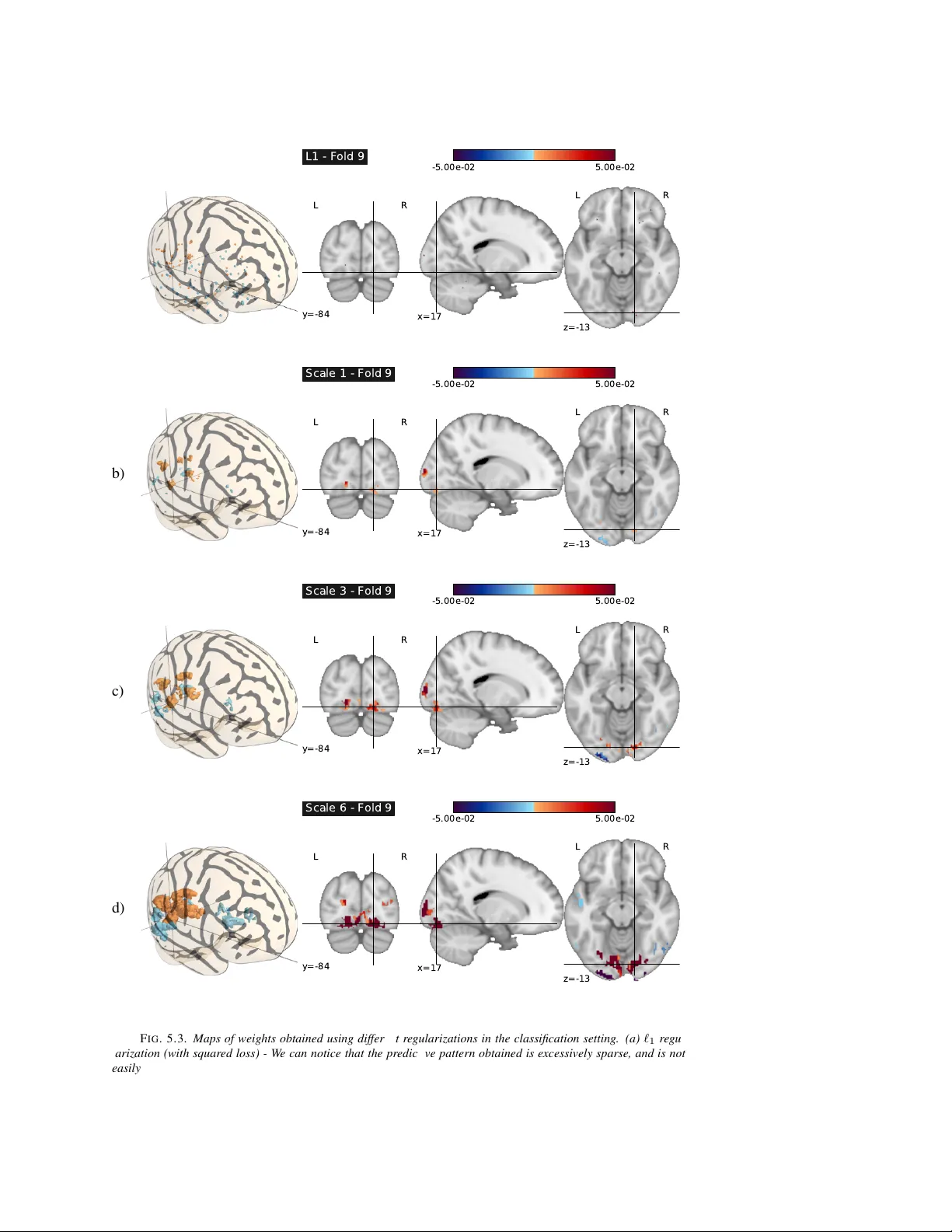
MUL TI-SCALE MINING OF FMRI D A T A WITH HIERARCHICAL STR UCTURED SP ARSITY R ODOLPHE JEN A TTON ∗ , ALEXANDRE GRAMFOR T † , VINCENT MICHEL † , GUILLA UME OBOZINSKI ∗ , EVEL YN EGER ‡ , FRANCIS B A CH ∗ , AND BER TRAND THIRION † Abstract. Rev erse inference, or “brain r eading” , is a recent paradigm for analyzing functional magnetic res- onance imaging (fMRI) data, based on pattern recognition and statistical learning. By predicting some cognitiv e variables related to brain activ ation maps, this approach aims at decoding brain activity . Rev erse inference takes into account the multi variate information between vox els and is currently the only w ay to assess ho w precisely some cognitiv e information is encoded by the activity of neural populations within the whole brain. Howev er , it relies on a prediction function that is plagued by the curse of dimensionality , since there are far more features than samples, i.e. , more voxels than fMRI volumes. T o address this problem, different methods hav e been proposed, such as, among others, univ ariate feature selection, feature agglomeration and regularization techniques. In this paper , we consider a sparse hierarchical structured regularization. Specifically , the penalization we use is constructed from a tree that is obtained by spatially-constrained agglomerative clustering. This approach encodes the spatial structure of the data at different scales into the regularization, which makes the ov erall prediction procedure more robust to inter-subject variability . The regularization used induces the selection of spatially coherent predictiv e brain regions simultaneously at different scales. W e test our algorithm on real data acquired to study the mental representation of objects, and we show that the proposed algorithm not only delineates meaningful brain regions but yields as well better prediction accuracy than reference methods. Key words. brain reading, structured sparsity , conv ex optimization, sparse hierarchical models, inter-subject validation, proximal methods. AMS subject classifications. - 1. Introduction. Functional magnetic resonance imaging (or fMRI) is a widely used functional neuroimaging modality . Modeling and statistical analysis of fMRI data are com- monly done through a linear model, called general linear model (GLM) in the community , that incorporates information about the different experimental conditions and the dynamics of the hemodynamic response in the design matrix. The experimental paradigm consists of a sequence of stimuli, e.g. , visual and auditory stimuli, which are included as regressors in the design matrix after conv olution with a suitable hemodynamic filter . The resulting model parameters—one coefficient per vox el and regressor —are known as activation maps . The y represent the local influence of the different experimental conditions on fMRI signals at the lev el of individual voxels. The most commonly used approach to analyze these activ ation maps is called classical inference. It relies on mass-uni variate statistical tests (one for each vox el), and yields so-called statistical parametric maps (SPMs) [19]. Such maps are useful for functional brain mapping, but classical inference has some limitations: it suf fers from mul- tiple comparisons issues and it is obli vious of the multiv ariate structure of fMRI data. Such data exhibit natural correlations between neighboring vox els forming clusters with different sizes and shapes, and also between distant but functionally connected brain re gions. T o address these limitations, an approach called reverse inference (or “brain-reading”) [14, 13] was recently proposed. Re verse inference relies on pattern recognition tools and statis- tical learning methods to explore fMRI data. Based on a set of acti vation maps, re verse inference estimates a function that can then be used to predict a target (typically , a variable representing a perceptual, cognitiv e or behavioral parameter) for a new set of images. The ∗ INRIA Rocquencourt - Sierra Project-T eam, Laboratoire d’Informatique de l’Ecole Normale Sup ´ erieure, IN- RIA/ENS/CNRS UMR 8548 ( firstname.lastname@inria.fr ). † INRIA Saclay - Parietal Project-T eam, CEA Neurospin. ( firstname.lastname@inria.fr ). ‡ INSERM U562, France - CEA/ DSV/ I2BM/ Neurospin/ Unicog ( evelyn.eger@cea.fr ). 0 A preliminary version of this work appeared in [27]. 1 2 R. Jenatton, A. Gramfort, V . Michel, G. Obozinski, E. Eger , F . Bach and B. Thirion challenge is to capture the correlation structure present in the data in order to improve the accuracy of the fit, which is measured through the resulting prediction accuracy . Many stan- dard statistical learning approaches hav e been used to construct prediction functions, among them kernel machines (SVM, R VM) [54] or discriminant analysis (LD A, QD A) [22]. For the application considered in this paper , earlier performance results [13, 32] indicate that we can restrict ourselves to mappings that are linear functions of the data. Throughout the paper , we shall consider a training set composed of n pairs ( x , y ) ∈ R p × Y , where x denotes a p -dimensional fMRI signal ( p voxels) and y stands for the target we try to predict. Each fMRI data point x will correspond to an activ ation map after GLM fitting. In the e xperiments we carry out in Section 5, we will encounter both the regression and the multi-class classification settings, where Y denotes respectively the set of real numbers and a finite set of integers. An example of a regression setting is the prediction of a pain le vel from fMRI data [37] or in the context of classification, the prediction of object categories [13]. T ypical datasets consists of a fe w hundreds of measurements defined each on a 2 × 2 × 2 -mm vox els grid forming p ≈ 10 5 vox els when working with full brain data. Such numbers, giv en as illustration, are not intrinsic limitation of MRI technology and are still re gularly improv ed by experts in the field. In this paper, we aim at learning a weight vector w ∈ R p and an intercept b ∈ R such that the prediction of y can be based on the value of w > x + b . This is the case for the linear regression and logistic regression models that we use in Section 5. The scalar b is not particularly informativ e, howe ver the vector w corresponds to a volume that can be represented in brain space as a v olume for visualization of the predicti ve pattern of v oxels. It is useful to rewrite these quantities in matrix form; more precisely , we denote by X ∈ R n × p the design matrix assembled from n fMRI volumes and by y ∈ R n the corresponding n targets. In other words, each ro w of X is a p -dimensional sample, i.e. , an acti vation map of p vox els related to one stimulus presentation. Learning the parameters ( w , b ) remains challenging since the number of features ( 10 4 to 10 5 vox els) exceeds by far the number of samples (a few hundreds of volumes). The prediction function is therefore prone to overfitting in which the learning set is predicted precisely whereas the algorithm provides very inaccurate predictions on new samples (the test set). T o address this issue, dimensionality reduction attempts to find a lo w dimensional subspace that concentrates as much of the predictive po wer of the original set as possible for the problem at hand. Feature selection is a natural approach to perform dimensionality reduction in fMRI, since reducing the number of voxels makes it easier to identify a predictiv e region of the brain. This corresponds to discarding some columns of X . This feature selection can be uni- variate, e.g. , analysis of v ariance (ANO V A) [33], or multiv ariate. While univ ariate methods ignore joint information between features, multiv ariate approaches are more adapted to re- verse inference since the y extract predicti ve patterns from the data as a whole. Howe ver , due to the huge number of possible patterns, these approaches suffer from combinatorial explo- sion, and some costly suboptimal heuristics ( e.g . , recursiv e feature elimination [21, 39]) can be used. That is why ANO V A is usually preferred in fMRI. Alternatively , two more adapted solutions hav e been proposed: r e gularization and featur e agglomer ation . Regularization is a way to encode a priori knowledge about the weight vector w . Pos- sible regularizers can promote for example spatial smoothness or sparsity which is a natural assumption for fMRI data. Indeed, only a few brain regions are assumed to be significantly activ ated during a cognitiv e task. Previous contributions on fMRI-based re verse inference include [6, 51, 52, 64]. They can be presented through the follo wing minimization problem: min ( w ,b ) ∈ R p +1 L ( y , X , w , b ) + λ Ω( w ) with λ ≥ 0 , (1.1) Multi-scale Mining of fMRI Data with Hierarchical Structured Sparsity 3 where λ Ω( w ) is the regularization term, typically a non-Euclidean norm, and the fit to the data is measured through a conv ex loss function ( w , b ) 7→ L ( y , X , w , b ) ∈ R + . The choice of the loss function will be made more specific and formal in the next sections. The coef- ficient of regularization λ balances the loss and the penalization term. In this notation, a common regularization term in rev erse inference is the so-called Elastic net [67, 20], which is a combined ` 1 and ` 2 penalization: λ Ω( w ) = λ 1 k w k 1 + λ 2 k w k 2 2 = p X j =1  λ 1 | w j | + λ 2 w 2 j  . (1.2) For the squared loss, when setting λ 1 to 0, the model is called ridge regression, while when λ 2 = 0 it is known as Lasso [58] or basis pursuit denoising (BPDN) [9]. The essential shortcoming of the Elastic net is that it does not take into account the spatial structure of the data, which is crucial in this context [43]. Indeed, due to the intrinsic smoothing of the complex metabolic pathway underlying the difference of blood oxygenation measured with fMRI [61], statistical learning approaches should be informed by the 3D grid structure of the data. In order to achiev e dimensionality reduction, while taking into account the spatial struc- ture of the data, one can resort to feature agglomer ation . Precisely , ne w features called par cels are naturally generated via av eraging of groups of neighboring vox els exhibiting similar activ ations. The advantage of agglomeration is that no information is discarded a priori and that it is reasonable to hope that averaging might reduce noise. Although, this ap- proach has been successfully used in pre vious work for brain mapping [18, 57], existing work does typically not consider the supervised information ( i.e. , the target y ) while exploring the parcels. A recent approach has been proposed to address this issue, based on a supervised greedy top-down exploration of a tree obtained by hierarchical clustering [42]. This greedy approach has proven to be ef fectiv e especially for inter-subject analyzes, i.e. , when training and ev aluation sets are related to different subjects. In this context, methods need to be robust to intrinsic spatial v ariations that exist across subjects: although a preliminary co-registration to a common space has been performed, some variability remains between subjects, which implies that there is no perfect vox el-to-vox el correspondence between volumes. As a result, the performances of traditional vox el-based methods are strongly af fected. Therefore, aver - aging in the form of parcels is a good way to cope with inter-subject variability . This greedy approach is nonetheless suboptimal, as it explores only a subpart of the whole tree. Based on these considerations, we propose to integrate the multi-scale spatial structure of the data within the regularization term Ω , while preserving conv exity in the optimization. This notably guarantees global optimality and stability of the obtained solutions. T o this end, we design a sparsity-inducing penalty that is directly built from the hierarchical structure of the spatial model obtained by W ard’ s algorithm [62] using a contiguity-constraint [45]. This kind of penalty has already been successfully applied in se veral contexts, e.g . , in bioinformat- ics, to exploit the tree structure of gene networks for multi-task regression [30], in log-linear models for the selection of potential orders [53], in image processing for wav elet-based de- noising [3, 28, 49], and also for topic models [28]. Other applications have emerged in natural language [40] and audio processing [55]. W e summarize here the contributions of our paper: • W e explain how the multi-scale spatial structure of fMRI data can be taken into account in the context of re verse inference through the combination of a spatially constrained hierarchical clustering procedure and a sparse hierarchical regulariza- tion. 4 R. Jenatton, A. Gramfort, V . Michel, G. Obozinski, E. Eger, F . Bach and B. Thirion • W e provide a con ve x formulation of the problem and propose an efficient optimiza- tion procedure. • W e conduct an experimental comparison of sev eral algorithms and formulations on fMRI data and illustrate the ability of the proposed method to localize in space and in scale some brain regions in volv ed in the processing of visual stimuli. The rest of the paper is organized as follo ws: we first present the concept of structured sparsity-inducing regularization and then describe the different regression/classification for- mulations we are interested in. After exposing how we handle the resulting large-scale con vex optimization problems thanks to a particular instance of proximal methods—the forward- backward splitting algorithm, we validate our approach both in a synthetic setting and on a real dataset. 2. Combining agglomerativ e clustering with sparsity-inducing regularizers. As sug- gested in the introduction, it is possible to construct a tree-structured hierarchy of new features on top of the original vox els using hierarchical clustering. Moreover , spatial constraints can be enforced in the clustering algorithm so that the underlying voxels corresponding to each of these features form localized spatial patterns on the brain similar to the ones we hope to re- triev e [10]. Once these features constructed, instead of selecting features in the tree greedily , we propose to cast the feature selection problem as supervised learning problem of the form (1.1). One of the qualities of the greedy approach howe ver is that it is only allowed to select potentially more noisy features, corresponding to smaller clusters, after the a priori more sta- ble features associated with ancestral clusters in the hierarch y ha ve been selected. As we will show , it is possible to construct a conv ex regularizer Ω that has the same property , i.e. that respects the hierarchy , and prioritizes the selection of features in the same way . Naturally , the regularizer has to be constructed directly from the hierarchical clustering of the v oxels. 2.1. Spatially-constrained hierarchical clustering. Starting from n fMRI volumes X = [ x 1 , . . . , x p ] ∈ R n × p described by p voxels, we seek to cluster these vox els so as to produce a hierarchical representation of X . T o this end, we consider hierar chical agglomerative clustering procedures [29]. These begin with e very vox el x j representing a singleton cluster { j } , and at each iteration, a selected pair of clusters—according to a criterion discussed below—is merged into a single cluster . This procedure yields a hierarchy of clusters represented as a binary tree T (also often called a dendrogram) [29], where each nonterminal node is associated with the cluster obtained by merging its two children clusters. Moreover , the root of the tree T is the unique cluster that gathers all the v oxels, while the leav es are the clusters consisting of a single v oxel. From no w on, we refer to each nonterminal node of T as a parcel , which is the union of its children’ s vox els (see Figure 2.1). Among different hierarchical agglomerativ e clustering procedures, we use the variance- minimizing approach of W ard’ s algorithm [62]. In short, two clusters are merged if the result- ing cluster minimizes the sum of squared differences of the fMRI signal within all clusters (also kno wn as inertia criterion ). More formally , at each step of the procedure, we merge the clusters c 1 and c 2 that minimize the criterion ∆( c 1 , c 2 ) = X j ∈ c 1 ∪ c 2 k x j − h X i c 1 ∪ c 2 k 2 2 −  X j ∈ c 1 k x j − h X i c 1 k 2 2 + X k ∈ c 2 k x k − h X i c 2 k 2 2  = | c 1 || c 2 | | c 1 | + | c 2 | kh X i c 1 − h X i c 2 k 2 2 , (2.1) where we have introduced the av erage vector h X i c , 1 | c | P j ∈ c x j . In order to take into account the spatial information, we also add connecti vity constraints in the hierarchical clus- Multi-scale Mining of fMRI Data with Hierarchical Structured Sparsity 5 tering algorithm, so that only neighboring clusters can be merged together . In other words, we try to minimize the criterion ∆( c 1 , c 2 ) only for pairs of clusters which share neighbor- ing vox els (see Algorithm 1). This connectedness constraint is important since the resulting clustering is likely to dif fer from standard W ard’ s hierarchical clustering. F I G . 2 . 1. Example of a tr ee T when p = 5 , with three voxels and two parcels. The par cel 2 is de- fined as the averaged intensity of the voxels { 1 , 2 } , while the parcel 1 is obtained by averaging the val- ues of the voxels { 1 , 2 , 3 } . In r ed dashed lines are r epresented the five gr oups of variables that com- pose G . F or instance, if the group containing the par cel 2 is set to zer o, the voxels { 1 , 2 } are also (and necessarily) zer oed out. Best seen in color . P ar c el 1 P ar c el 2 V o x el 1 V o x el 2 V o x el 3 2.1.1. A ugmented space of featur es. Based on the output of the hierarchical clustering presented previously , we define the following augmented space of variables (or featur es ): instead of representing the n fMRI volumes only by its individual vox el intensities, we add to it a vector with lev els of activ ation of each of the parcels at the interior nodes of the tree T , which we obtained from the agglomerativ e clustering algorithm. Since T has q , |T | = 2 p − 1 nodes, 1 , the data obtained in the augmented space can be gathered in a matrix ˜ X ∈ R n × q . In the following, the lev el of activ ation of each parcel is simply the averaged intensity of the voxels it is composed of ( i.e. , local averages) [18, 57]. This produces a multi-scale representation of the fMRI data that has the advantage of becoming increasingly inv ariant to spatial shifts of the encoding regions within the brain volume. W e summarize the procedure to build the enlar ged matrix ˜ X ∈ R n × q in Algorithm 1. Let us now illustrate on the example Algorithm 1 Spatially-constrained agglomerativ e clustering and augmented feature space. Input: n fMRI volumes X = [ x 1 , . . . , x p ] ∈ R n × p described by p vox els. Output: n fMRI volumes ˜ X ∈ R n × q in the augmented feature space. Initialization: C =  { j } ; j ∈ { 1 , . . . , p }  , ˜ X = X . while |C | > 1 do Find a pair of clusters c 1 , c 2 ∈ C which have neighboring v oxels and minimize (2.1). C ← C \ { c 1 , c 2 } . C ← C ∪ ( c 1 ∪ c 2 ) . ˜ X ← [ ˜ X , h X i c 1 ∪ c 2 ] . end while Return: ˜ X . of linear models (such as those we use in Section 3) what are the implications of considering the augmented space of features. For a node j of T , we let denote by P j ⊆ { 1 , . . . , p } the set of vox els of the corresponding parcel (or , equiv alently , the set of leaves of the subtree rooted 1 W e can then identify nodes (and parcels) of T with indices in { 1 , . . . , q } . 6 R. Jenatton, A. Gramfort, V . Michel, G. Obozinski, E. Eger, F . Bach and B. Thirion at node j ). In this notation, and for any fMRI volume ˜ x ∈ R q in the augmented feature space, linear functions index ed by w ∈ R q take the form f w ( ˜ x ) = w > ˜ x = q X j =1 w j h 1 | P j | X k ∈ P j x k i = p X k =1 h X j ∈ A k w j | P j | i x k , where A k stands for the set of ancestors of a node k in T (including itself). 2.2. Hierarchical sparsity-inducing norms. In the perspectiv e of inter-subject vali- dation, the augmented space of variables can be exploited in the following way: Since the information of single voxels may be unreliable, the deeper the node in T , the more variable the corr esponding parcel’ s intensity is likely to be acr oss subjects . This property suggests that, while looking for sparse solutions of (1.1), we should preferentially select the variables near the root of T , before trying to access smaller parcels located further down in T . T raditional sparsity-inducing penalties, e.g . , the ` 1 -norm Ω( w ) = P p j =1 | w j | , yield sparsity at the level of single variables w j , disregarding potential structures—for instance, spatial—existing between larger subsets of variables. W e leverage here the concept of struc- tur ed sparsity [3, 7, 66, 24, 26, 25, 41, 16], where Ω penalizes some predefined subsets, or gr oups , of variables that reflect prior information about the problem at hand. When these groups form a partition of the space of variables, the resulting penalty has been sho wn to improve the prediction performance and/or interpretability of the learned mod- els, provided that the block structure is relev ant (e.g., see [60, 65, 35, 31, 56, 23] and refer- ences therein). If the groups overlap [3, 66, 24, 26, 25, 36], richer structures can then be encoded. In particular , we follow [66] who first introduced hierarchical sparsity-inducing penalties. Giv en a node j of T , we denote by g j ⊆ { 1 , . . . , q } the set of indices that record all the descendants of j in T , including itself. In other words, g j contains the indices of the subtree rooted at j ; see Figure 2.1. If we no w denote by G the set of all g j , j ∈ { 1 , . . . , q } , that is, G , { g 1 , . . . , g q } , we can define our hierarchical penalty as Ω( w ) , X g ∈G k w g k 2 , X g ∈G h X j ∈ g w 2 j i 1 / 2 . (2.2) As formally sho wn in [26], Ω is a norm on R q , and it promotes sparsity at the le vel of groups g ∈ G , in the sense that it acts as a ` 1 -norm on the vector ( k w g k 2 ) g ∈G . Regularizing by Ω therefore causes some k w g k 2 (and equi valently w g ) to be zeroed out for some g ∈ G . Moreov er , since the groups g ∈ G represent rooted subtrees of T , this implies that if one node/parcel j ∈ g is set to zero by Ω , the same occurs for all its descendants [66]. T o put it differently , if one par cel is selected, then all the ancestral par cels in T will also be selected . This property is likely to increase the robustness of the methods to voxel misalignments be- tween subjects, since large parcels will be considered for addition in the model before smaller ones. The family of norms with the previous property is actually slightly larger and we consider throughout the paper norms Ω of the form [66]: Ω( w ) , X g ∈G η g k w g k , (2.3) where k w g k denotes either the ` 2 -norm k w g k 2 or the ` ∞ -norm k w g k ∞ , max j ∈ g | w j | and ( η g ) g ∈G are (strictly) positi ve weights that can compensate for the fact that some features are Multi-scale Mining of fMRI Data with Hierarchical Structured Sparsity 7 ov erpenalized as a result of being included in a larger number of groups than others. In light of the results from [28], we will see in Section 4 that a large class of optimization problems regularized by Ω —as defined in (2.3)— can be solv ed efficiently . 3. Supervised learning framework. In this section, we introduce the formulations we consider in our experiments. As further discussed in Section 5, the target y we try to pre- dict corresponds to (discrete) sizes of objects, i.e. , a one-dimensional or der ed variable. It is therefore sensible to address this prediction task from both a regression and a classification viewpoint. In the remainder of this section, we shall denote by { w ∗ , b ∗ } (or { W ∗ , b ∗ } ) a solution of the optimization problems we present belo w . 2 For simplicity , the formulations we revie w next are all expressed in terms of a matrix X ∈ R n × p with p -dimensional param- eters, but they are of course immediately applicable to the augmented data ˜ X ∈ R n × q and q -dimensional parameters. 3.1. Regression. In this first setting, we naturally consider the squared loss function, so that problem (1.1) can be reduced to min w ∈ R p 1 2 n k y − Xw k 2 2 + λ Ω( w ) with λ ≥ 0 . Note that in this case, we hav e omitted the intercept b since we can center the vector y and the columns of X instead. Prediction for a new fMRI volume x is then simply performed by computing the dot product x > w ∗ . 3.2. Classification. W e can look at our prediction task from a multi-class classification viewpoint. Specifically , we assume that Y is a finite set of integers { 1 , . . . , c } , c > 2 , and consider both multi-class and “one-versus-all” strate gies [50]. W e need to slightly e xtend the formulation (1.1): T o this end, we introduce the weight matrix W , [ w 1 , . . . , w c ] ∈ R p × c , composed of c weight vectors, along with a vector of intercepts b ∈ R c . A standard way of addressing multi-class classification problems consists in using a multi-logit model, also known as multinomial logistic regression (see, e.g . , [22] and refer- ences therein). In this case, class-conditional probabilities are modeled for each class by a softmax function, namely , giv en a fMRI volume x , the probability of having the k -th class label reads Prob ( y = k | x ; W , b ) = exp { x > w k + b k } P c r =1 exp { x > w r + b r } for k ∈ { 1 , . . . , c } . (3.1) The parameters { W , b } are then learned by maximizing the resulting (conditional) log- likelihood, which leads to the follo wing optimization problem: min W ∈ R p × c b ∈ R c 1 n n X i =1 log h c X k =1 e x > i ( w k − w y i )+ b k − b y i i + λ c X k =1 Ω( w k ) . Whereas the regularization term is separable with respect to the different weight vectors w k , the loss function induces a coupling in the columns of W . As a result, the optimization has to be carried out ov er the entire matrix W . In this setting, and given a new fMRI volume x , we make predictions by choosing the label that maximizes the class-conditional probabil- ities (3.1), that is, argmax k ∈{ 1 ,...,c } Prob ( y = k | x ; W ∗ , b ∗ ) . In Section 5, we consider another multi-class classification scheme. The “one-versus-all” strategy (O V A) consists in training c different (real-valued) binary classifiers, each one being 2 In the absence of strong con vexity , we cannot in general guarantee the uniqueness of w ∗ (and W ∗ ). 8 R. Jenatton, A. Gramfort, V . Michel, G. Obozinski, E. Eger, F . Bach and B. Thirion trained to distinguish the examples in a single class from the observations in all remaining classes. In order to classify a new example, among the c classifiers, the one which outputs the largest (most positiv e) value is chosen. In this frame work, we consider binary classifiers built from both the squared and the logistic loss functions. If we denote by ¯ Y ∈ {− 1 , 1 } n × c the indicator response matrix defined as ¯ Y k i , 1 if y i = k and − 1 otherwise, we obtain min W ∈ R p × c 1 2 n c X k =1 k ¯ Y k − Xw k k 2 2 + λ c X k =1 Ω( w k ) , and min W ∈ R p × c b ∈ R c 1 n n X i =1 c X k =1 log h 1 + e − ¯ Y k i ( x > i w k + b k ) i + λ c X k =1 Ω( w k ) . By in voking the same ar guments as in Section 3.1, the v ector of intercepts b is again omitted in the above problem with the squared loss. Moreov er , giv en a new fMRI volume x , we predict the label k that maximizes the response x > [ w ∗ ] k among the c different classifiers. The case of the logistic loss function parallels the setting of the multinomial logistic regression, where each of the c “one-versus-all” classifiers leads to a class-conditional probability; the predicted label is the one corresponding to the highest probability . The formulations we have revie wed in this section can be solved efficiently within the same optimization framew ork that we now introduce. 4. Optimization. The con ve x minimization problem (1.1) is challenging, since the penalty Ω as defined in (2.3) is non-smooth and the number of v ariables to consider is lar ge (we ha ve q ≈ 10 5 variables in the following experiments). These difficulties are well addressed by forwar d-backwar d splitting methods , which belong to the broader class of proximal methods. Forward-backw ard splitting schemes date back (at least) to [38, 34] and ha ve been further analyzed in various settings (e.g., see [59, 8, 12]); for a thorough re view of proximal splitting techniques, we refer the interested readers to [11]. Our conv ex minimization problem (1.1) can be handled well by such techniques since it is the sum of two semi-lower continuous, proper , con vex functions with non-empty domain, and where one element—the loss function L ( y , X , . ) —is assumed differentiable with Lipschitz- continuous gradient (which notably cov ers the cases of the squared and simple/multinomial logistic functions, as introduced in Section 3). T o describe the principle of forward-backward splitting methods, we need to introduce the concept of proximal operator . The proximal operator associated with our regularization term λ Ω , which we denote by Prox λ Ω , is the function that maps a vector w ∈ R p to the unique solution of min v ∈ R p 1 2 k v − w k 2 2 + λ Ω( v ) . (4.1) This operator was initially introduced by Moreau [44] to generalize the projection operator onto a con ve x set; for a complete study of the properties of Prox λ Ω , see [12]. Based on defi- nition (4.1), and giv en the current iterate w ( k ) , 3 the typical update rule of forward-backward splitting methods has the form 4 w ( k +1) ← Prox λ L Ω  w ( k ) − 1 L ∇L w ( y , X , w ( k ) )  , (4.2) 3 For clarity of the presentation, we do not consider the optimization of the intercept that we lea ve unregularized in all our experiments. 4 For simplicity , we only present a constant-stepsize scheme; adaptive line search can also be used in this context and can lead to larger stepsizes [11]. Multi-scale Mining of fMRI Data with Hierarchical Structured Sparsity 9 where L > 0 is a parameter which is a upper bound on the Lipschitz constant of the gradient of L . In the light of the update rule (4.2), we can see that solving efficiently problem (4.1) is crucial to enjoy good performance. In addition, when the non-smooth term Ω is not present, the previous proximal problem (4.2), also known as the implicit or backward step, exactly leads to the standard gradient update rule. For many regularizations Ω of interest, the solution of problem (4.1) can actually be computed in closed form in simple settings: in particular, when Ω is the ` 1 -norm, the proximal operator is the well-kno wn soft-thresholding operator [15]. The work of [28] recently sho wed that the proximal problem (4.1) could be solved efficiently and exactly with Ω as defined in (2.3). The underlying idea of this computation is to solve a well-or der ed sequence of simple proximal problems associated with each of the terms k w g k for g ∈ G . W e refer the interested readers to [28] for further details on this norm and to [2] for a broader view . In the subsequent experiments, we focus on accelerated multi-step versions of forward- backward splitting methods (see, e.g., [46, 4, 63]), 5 where the proximal problem (4.2) is not solved for a current estimate, b ut for an auxiliary sequence of points that are linear combina- tions of past estimates. These accelerated versions ha ve increasingly dra wn the attention of a broad research community since they can deal with large non-smooth conv ex problems, and their conv ergence rates on the objectiv e achiev e the complexity bound of O (1 /k 2 ) , with k denoting the iteration number . As a side comment, note that as opposed to standard one-step forward-backward splitting methods, nothing can be said about the con ver gence of the se- quence of iterates themselves. In our case, the cost of each iteration is dominated by the com- putation of the gradient ( e.g. , O ( np ) for the squared loss) and the proximal operator , whose time complexity is linear , or close to linear , in p for the tree-structured regularization [28]. 5. Experiments and results. W e now present experimental results on simulated data and real fMRI data. 5.1. Simulations. In order to illustrate the proposed method, the hierarchical regular- ization with the ` 2 -norm and η g = 1 for all g ∈ G was applied in a regression setting on a small two-dimensional simulated dataset consisting of 300 square images ( 40 × 40 pixels i.e. X ∈ R 300 × 1600 ). The weight vector w used in the simulation— itself an image of the same dimension— is presented in Fig. 5.1-a. It consists of three localized regions of two different sizes that are predictiv e of the output. The images x ( i ) are sampled so as to obtain a correlation structure which mimics fMRI data. Precisely , each image x ( i ) was obtained by smoothing a completely random image — where each pixel was drawn i.i.d from a normal distribution — with a Gaussian kernel (standard de viation 2 pixels), which introduces spatial correlations between neighboring pixels. Subsequently , additional correlations between the regions corresponding to the three patterns were introduced in order to simulate co-activ ations between dif ferent brain regions, by multiplying the signal by the square-root of an appropriate cov ariance matrix Σ . Specifically , Σ ∈ R 1600 × 1600 is a spatial covariance between vox els, with diagonal set to Σ i,i = 1 for all i , and with tw o of f-diagonal blocks. Let us denote C 1 and C 2 the set of voxels forming the two larger patterns, and C 3 the vox els in the small pattern. The cov ariance coefficients are set to Σ i,j = 0 . 3 for i ∈ C 1 and j ∈ C 2 , and Σ i,j = − 0 . 2 for i ∈ C 2 and j ∈ C 3 . The cov ariance is of course symmetric. The choice of the weights and of the correlation introduced in images aim at illustrat- ing how the hierarchical regularization estimates weights at different resolutions in the im- age. The targets were simulated by forming w > x ( i ) corrupted with an additiv e white noise (SNR=10dB). The loss used was the squared loss as detailed in Section 3.1. The regular - 5 More precisely , we use the accelerated proximal gradient scheme (FIST A) taken from [4]. The Matlab/C++ implementation we use is av ailable at http://www.di.ens.fr/willow/SPAMS/ . 10 R. Jenatton, A. Gramfort, V . Michel, G. Obozinski, E. Eger, F . Bach and B. Thirion True a) Scale 1 b) Scale 2 c) Scale 3 d) Scale 4 e) Scale 5 f) Scale 6 g) Scale 7 h) F I G . 5 . 1. W eights w ∗ estimated in the simulation study . The true coefficients are presented in a) and the estimated weights at dif ferent scales, i.e., differ ent depths in the tr ee, ar e pr esented in b)-h) with the same colormap. The r esults are best seen in color . ization parameter was estimated with two-fold cross-validation (150 images per fold) on a logarithmic grid of 30 v alues between 10 3 and 10 − 3 . The components of the estimated weight vector w ∗ at different scales are presented in the images of Fig. 5.1 , with each image corresponding to a dif ferent depth in the tree. For a giv en tree depth, an image is formed from the corresponding parcellation. All the vox els within a parcel are colored according to the associated scalar in w ∗ . It can be observed that all three patterns are present in the weight vector but at dif ferent depths in the tree. The small activ ation in the top-right hand corner sho ws up mainly at scale 3 while the bigger patterns appear higher in the tree at scales 5 and 6. This simulation clearly illustrates the ability of the method to capture informativ e spatial patterns at different scales. 5.2. Description of the fMRI data. W e apply the dif ferent methods to analyze the data of ten subjects from an fMRI study originally designed to in vestigate object coding in visual cortex (see [17] for details). During the experiment, ten healthy volunteers viewed objects of two categories (each one of the two categories is used in half of the subjects) with four different ex emplars in each category . Each ex emplar was presented at three different sizes (yielding 12 different experimental conditions per subject). Each stimulus was presented four times in each of the six sessions. W e averaged data from the four repetitions, resulting in a total of n = 72 volumes by subject (one volume of each stimulus by session). Functional volumes were acquired on a 3-T MR system with eight-channel head coil (Siemens Trio, Erlangen, Germany) as T2*-weighted echo-planar image (EPI) volumes. T wenty transverse slices were obtained with a repetition time of 2s (echo time, 30ms; flip angle, 70 ◦ ; 2 × 2 × 2 - mm v oxels; 0 . 5 -mm gap). Realignment, spatial normalization to MNI space, slice timing correction and GLM fit were performed with the SPM5 software 6 . In the GLM, the time course of each of the 12 stimuli con volv ed with a standard hemodynamic response function was modeled separately , while accounting for serial auto-correlation with an AR(1) model and removing low-frequenc y drift terms with a high-pass filter with a cut-of f of 128s ( 7 . 8 × 10 − 3 Hz). In the present work we used the resulting session-wise parameter estimate v olumes. 6 http://www.fil.ion.ucl.ac.uk/spm/software/spm5 . Multi-scale Mining of fMRI Data with Hierarchical Structured Sparsity 11 Contrary to a common practice in the field the data were not smoothed with an isotropic Gaussian filter . All the analysis are performed on the whole acquired volume. The four different exemplars in each of the two categories were pooled, leading to vol- umes labeled according to the three possible sizes of the object. By doing so, we are interested in finding discriminativ e information to predict the size of the presented object. This can be reduced to either a regression problem in which our goal is to predict the class label of the size of the presented object (i.e., y ∈ { 0 , 1 , 2 } ), 7 or a three-category classification problem, each size corresponding to a category . W e perform an inter-subject analysis on the sizes both in regression and classification settings. This analysis relies on subject-specific fixed-ef fects activ ations, i.e. , for each condition, the six activ ation maps corresponding to the six sessions are a veraged together . This yields a total of 12 volumes per subject, one for each experimental condition. The dimensions of the real data set are p ≈ 7 × 10 4 and n = 120 (divided into three different sizes). W e ev aluate the performance of the method by cross-validation with a natural data splitting, leave-one-subject-out . Each fold consists of 12 volumes. The parameter λ of all methods is optimized over a grid of 30 v alues of the form 2 k , with a nested leav e-one-subject-out cross-v alidation on the training set. The exact scaling of the grid varies for each model to account for dif ferent Ω . 5.3. Methods in volved in the comparisons. In addition to considering standard ` 1 - and squared ` 2 -regularizations in both our regression and multi-class classification tasks, we compare various methods that we no w revie w . First of all, when the regularization Ω as defined in (2.3) is employed, we consider three settings of values for ( η g ) g ∈G which lev erage the tree structure T . More precisely , we set η g = ρ depth ( g ) for g in G , with ρ ∈ { 0 . 5 , 1 , 1 . 5 } and where depth ( g ) denotes the depth of the root of the group g in T . In other words, the larger ρ , the more averse we are to selecting small (and variable) parcels located near the leaves of T . As the results illustrate it, the choice of ρ can ha ve a significant impact on the performance. More generally , the problem of selecting ρ properly is a dif ficult question which is still under in vestigation, both theoretically and practically , e.g., see [1]. The greedy approach from [42] is included in the comparisons, for both the regression and classification tasks. It relies on a top-down exploration of the tree T . In short, start- ing from the root parcel that contains all the voxels, we choose at each step the split of the parcel that yields the highest prediction score. The exploration step is performed until a giv en number of parcels is reached, and yields a set of nested parcellations with increasing complexity . Similarly to a model selection step, we chose the best parcellation among those found in the exploration step. The selected parcellation is thus used on the test set. In the regression setting, this approach is combined with Bayesian ridge regression, while it is as- sociated with a linear support vector machine for the classification task (whose re gularization parameter , often referred to as C in the literature [54], is found by nested cross-validation in { 0 . 01 , 0 . 1 , 1 } ). 5.3.1. Regression setting. In order to ev aluate whether the lev el of sparsity is critical in our analysis, we implemented a re weighted ` 1 -scheme [5]. In this case, sparsity is encour - aged more aggressi vely as a multi-stage con vex relaxation of a concav e penalty . Specifically , it consists in using iterati vely a weighted ` 1 -norm, whose weights are determined by the so- lution of previous iteration. Moreov er , we additionally compare to Elastic net [67], whose second regularization parameter is set by cross-validation as a fraction of λ , that is, αλ with α ∈ { 0 . 5 , 0 . 05 , 0 . 005 , 0 . 0005 } . 7 An interesting alternative would be to consider some real-valued dimension such as the field of view of the object. 12 R. Jenatton, A. Gramfort, V . Michel, G. Obozinski, E. Eger, F . Bach and B. Thirion T o better understand the added value of the hierarchical norm (2.3) over unstructured penalties, we not only consider the plain ` 1 -norm in the augmented feature space, but also another variant of weighted ` 1 -norm. The weights are manually set and reflect the under- lying tree structure T . By analogy with the choice of ( η g ) g ∈G made for the tree-structured regularization, we take exponential weights depending on the depth of the variable j , where η j = ρ depth ( j ) with ρ ∈ { 0 . 5 , 1 . 5 } . 8 W e also tried weights ( η j ) j ∈{ 1 ,...,p } that are linear with respect to the depths, i.e., η j = depth ( j ) max k ∈{ 1 ,...,p } depth ( k ) , but those led to worse results. In T able 5.1, we only present the best result of this weighted ` 1 -norm, obtained with the ex- ponential weight and ρ = 1 . 5 . W e now turn to the models taking part in the classification task. 5.3.2. Classification setting. As discussed in Section 3.2, the optimization in the clas- sification setting is carried out ov er a matrix of weights W ∈ R p × c . This makes it possible to consider regularization schemes that couple the selection of variables across ro ws of that matrix. In particular , we apply ideas from multi-task learning [47] by vie wing each class as a task. More precisely , we use a regularization norm defined by Ω multi-task ( W ) , P p j =1 k W j k , where k W j k denotes either the ` 2 - or ` ∞ -norm of the j -th ro w of W . The rationale for the definition of Ω multi-task is to assume that the set of relev ant voxels is the same across the c different classes, so that sparsity is induced simultaneously ov er the columns of W . It should be noted that , in the “one-versus-all” setting, although the loss functions for the c classes are decoupled, the use of Ω multi-task induces a relationship that ties the optimization problems together . Note that the tree-structured regularization Ω we consider does not impose a joint pattern- selection across the c dif ferent classes. It would howe ver be possible to use Ω over the matrix W , in a multi-task setting. More precisely , we would define Ω( W ) = P g ∈G k W g k , where k W g k denotes either the ` 2 - or ` ∞ -norm of the vectorized sub-matrix W g , [ W j k ] j ∈ g,k ∈{ 1 ,...,c } . This definition constitutes a direct extension of the standard non-overlapping ` 1 /` 2 - and ` 1 /` ∞ -norms used for multi-task. Furthermore, it is worth noting that the optimization tools from [28] would still apply for this tree-structured matrix regularization. 5.4. Results. W e present results comparing our approach based on the hierarchical sparsity-inducing norm (2.3) with the regularization listed in the previous section. For each method, we computed the cross-validated prediction accuracy and the percentage of non-zero coefficients, i.e . , the level of sparsity of the model. 5.4.1. Regression results. The results for the inter-subject regression analysis are re- ported in T able 5.1. The lowest error in prediction accuracy is obtained by both the greedy strategy and the proposed hierarchical structured sparsity approach (Tree ` 2 with ρ = 1 ) whose performances are essentially indistinguishable. Both also yield one of the lo west stan- dard deviation indicating that the results are most stable. This can be explained by the fact that the use of local signal averages in the proposed algorithm is a good way to get some robustness to inter-subject variability . W e also notice that the sparsity-inducing approaches (Lasso and re weighted ` 1 ) have the highest error in prediction accuracy , probably because the obtained solutions are too sparse, and suffer from the absence of perfect voxel-to-v oxel correspondences between subjects. In terms of sparsity , we can see, as expected, that ridge regression does not yield any sparsity and that the Lasso solution is very sparse (in the feature space, with approximately 8 Formally , the depth of the feature j is equal to depth ( g j ) , where g j is the smallest group in G that contains j ( smallest is understood here in the sense of the inclusion). Multi-scale Mining of fMRI Data with Hierarchical Structured Sparsity 13 Loss function: Squared loss Error (mean,std) P-value w .r.t. Tree ` 2 ( ρ = 1 ) Median fraction of non-zeros (%) Regularization: ` 2 (Ridge) (13.8, 7.6) 0.096 100.00 ` 1 (20.2, 10.9) 0.013 ∗ 0.11 ` 1 + ` 2 (Elastic net) (14.4, 8.8) 0.065 0.14 Reweighted ` 1 (18.8, 14.6) 0.052 0.10 ` 1 (augmented space) (14.2, 7.9) 0.096 0.02 ` 1 (tree weights) (13.9, 7.9) 0.032 ∗ 0.02 T ree ` 2 ( ρ = 0 . 5 ) (13.0, 7.4) 0.137 99.99 T ree ` 2 ( ρ = 1 ) ( 11.8 , 6.7 ) - 9.36 T ree ` 2 ( ρ = 1 . 5 ) (13.5, 7.0) 0.080 0.04 T ree ` ∞ ( ρ = 0 . 5 ) (13.6, 7.8) 0.080 99.99 T ree ` ∞ ( ρ = 1 ) (12.8, 6.7) 0.137 1.22 T ree ` ∞ ( ρ = 1 . 5 ) (13.0, 6.8) 0.096 0.04 Error (mean,std) P-value w .r.t. Tree ` 2 ( ρ = 1 ) Median fraction of non-zeros (%) Greedy (12.0, 5.5) 0.5 0.01 T A B L E 5 . 1 Pr ediction results obtained on fMRI data (see text) for the re gression setting. Fr om the left, the first column contains the mean and standard deviation of the test error (mean squared err or), computed over leave-one-subject- out folds. The best performance is obtained with the greedy technique and the hierar chical ` 2 penalization ( ρ = 1 ) constructed from the W ard tr ee. Methods with performance significantly worse than the latter is assessed by W ilcoxon two-sample paired signed rank tests (The superscript ∗ indicates a rejection at 5% ). Levels of sparsity reported ar e in the augmented space whenever it is used. 7 × 10 4 vox els). Our method yields a median value of 9.36% of non-zero coefficients (in the augmented space of features, with about 1 . 4 × 10 5 nodes in the tree). The maps of weights obtained with Lasso and the hierarchical regularization for one fold, are reported in Fig. 5.2. The Lasso yields a scattered and overly sparse pattern of vox els, that is not easily readable, while our approach extracts a pattern of vox els with a compact structure, that clearly outlines brain re gions expected to acti vate dif ferentially for stimuli with dif ferent low-le vel visual properties, e.g . , sizes; the early visual corte x in the occipital lobe at the back of the brain. Interestingly , the patterns of v oxels sho w some symmetry between left and right hemispheres, especially in the primary visual cortex which is located at the back and center of the brain. This observation is consistent with the current understanding in neuroscience that the symmetric parts of this brain re gion process respecti vely the visual contents of each of the visual hemifields. The weights obtained at different depth lev el in the tree, corresponding to different scales, sho w that the largest coefficients are concentrated at the higher scales (scale 6 in Fig. 5.2), which suggest that the object sizes cannot be well decoded at the voxel lev el but require features corresponding to lar ger clusters of vox els. 5.4.2. Classification results. The results for the inter-subject classification analysis are reported in T able 5.2. The best performance is obtained with a multinomial logistic loss function, also using the hierarchical ` 2 penalization ( ρ = 1 ). It should be noted that the sparsity level of the different model estimated vary widely depending on the loss and regularization used. W ith the squared loss, ` 1 type regularization, including the multi-task regularizations based on the ` 1 /` 2 and ` 1 /` ∞ norm tend to select quite sparse models, which keep around 0 . 1% of the v oxels. When using logistic type losses, these regularizations tend to select a significantly large number of vox els, which suggests that the selection problem is really difficult and that these methods are unstable. For the methods with hierarchical re gularization, on the contrary , the sparsity tends to improve with the choice 14 R. Jenatton, A. Gramfort, V . Michel, G. Obozinski, E. Eger, F . Bach and B. Thirion of loss functions that are better suited to the classification problem and tuning ρ trades off smoothly sparsity of the model against performance, from models that are not sparse when ρ is small to very sparse models when ρ is large. In particular a better compromise between sparsity and prediction performance can probably be obtained by tuning ρ ∈ [1 , 1 . 5] . For both ` 1 and hierarchical regularizations, one of the three vectors of coefficients ob- tained for one fold and for the loss leading to sparser models are presented in Fig. 5.3. For ` 1 , the activ e v oxels are scattered all o ver the brain, and for other losses than the squared-loss the models selected tend not to be sparse. By contrast, the tree ` 2 regularization yields clearly delineated sparsity patterns located in the visual areas of the brain. Like for the regression results, the highest coefficients are obtained at scale 6 showing how spatially extended is the brain region inv olved in the cognitiv e task. The symmetry of the pattern at this scale is also particularly striking in the primary visual areas. It also extends more anteriorly into the inferior temporal cortex, kno wn for high-level visual processing. 6. Conclusion. In this article, we introduced a hierarchically structured regularization, which takes into account the spatial and multi-scale structure of fMRI data. This approach copes with inter-subject v ariability in a similar way as feature agglomeration, by averaging neighboring voxels. Although alternativ e agglomeration strategies do exist, we simply used the criterion which appears as the most natural, W ard’ s clustering, and which builds parcels with little variance. Results on a real dataset show that the proposed algorithm is a promising tool for min- ing fMRI data. It yields similar or higher prediction accuracy than reference methods, and the map of weights it obtains exhibit a cluster-like structure. It makes them easily readable compared to the ov erly sparse patterns found by classical sparsity-promoting approaches. For the regression problem, both the greedy method from [42] and the proposed algo- rithm yield better results than unstructured and non-hierarchical regularizations, whereas in the classification setting, our approach leads to the best performance. Moreov er , our pro- posed methods enjoy the different benefits from con ve x optimization. In particular, while the greedy algorithm relies on a two-step approach that may be far from optimal, the hierar- chical regularization induces simultaneously the selection of the optimal parcellation and the construction of the optimal predictiv e model, given the initial hierarchical clustering of the vox els. Moreover , conv ex methods yield predictors that are essentially stable with respect to perturbations of the design or the initial clustering, which is typically not the case of greedy methods. It is important to distinguish here the stability of the predictors from that of the only learned map w , which could be enforced via a squared ` 2 -norm regularization. Finally , it should be mentioned that the performance achiev ed by this approach in inter- subject problems suggests that it could potentially be used successfully for medical diagnosis, in a context where brain images –not necessarily functional images– are used to classify indi- viduals into diseased or control population. Indeed, for difficult problems of that sort, where the reliability of the diagnostic is essential, the stability of models obtained from con vex formulations and the interpretability of sparse and localized solutions are quite relev ant to provide a credible diagnostic. Acknowledgments. The authors acknowledge support from the ANR grants V iMA G- INE ANR-08-BLAN-0250-02 and ANR 2010-Blan-0126-01 “IRMGroup”. The project was also partially supported by a grant from the European Research Council (SIERRA Project). REFERENCES [1] F . B AC H , High-dimensional non-linear variable selection thr ough hierarc hical kernel learning , tech. report, Preprint arXiv:0909.0844, 2009. Multi-scale Mining of fMRI Data with Hierarchical Structured Sparsity 15 [2] F . B AC H , R . J E NAT TO N , J . M A IR A L , A N D G . O B OZ I N S K I , Conve x optimization with sparsity-inducing norms , in Optimization for Machine Learning, S. Sra, S. Nowozin, and J. S. Wright, eds., MIT press, 2011. [3] R . G . B AR A N I U K , V . C E VH E R , M . F . D UA RT E , A N D C . H E G D E , Model-based compr essive sensing , IEEE T ransactions on Information Theory , 56 (2010), pp. 1982–2001. [4] A . B E C K A N D M . T E B O U LL E , A fast iterative shrinkage-thr esholding algorithm for linear in verse pr oblems , SIAM Journal on Imaging Sciences, 2 (2009), pp. 183–202. [5] E . J . C A N D E S , M . B . W A K I N , A N D S . P . B OY D , Enhancing spar sity by r eweighted L1 minimization , Journal of Fourier Analysis and Applications, 14 (2008), pp. 877–905. [6] M . K . C A R RO L L , G . A . C E CC H I , I . R I S H , R . G A R G , A N D A . R . R AO , Pr ediction and interpr etation of distributed neur al activity with sparse models , NeuroImage, 44 (2009), pp. 112 – 122. [7] V . C EV H E R , M . F. D UA RT E , C . H E G D E , A N D R . G . B A RA N I U K , Sparse signal reco very using markov random fields , in Adv ances in Neural Information Processing Systems, 2008. [8] G . H . G . C H E N A N D R . T. R O C K A FE L L A R , Con vergence rates in forward-bac kwar d splitting , SIAM Journal on Optimization, 7 (1997), pp. 421–444. [9] S . S . C H EN , D . L . D O N O HO , A N D M . A . S AU N DE R S , Atomic decomposition by basis pursuit , SIAM Journal on Scientific Computing, 20 (1998), pp. 33–61. [10] D . B . C H K L OV SK I I A N D A . A . K OU L A KOV , Maps in the brain: What can we learn from them? , Annual Revie w of Neuroscience, 27 (2004), pp. 369–392. [11] P . L . C O M B E TT E S A N D J . - C . P E S QU E T , Pr oximal splitting methods in signal processing , in Fixed-Point Algorithms for In verse Problems in Science and Engineering, Springer , 2010. [12] P . L . C O M BE T T E S A N D V . R . W A J S , Signal reco very by pr oximal forward-bac kward splitting , Multiscale Modeling and Simulation, 4 (2006), pp. 1168–1200. [13] D . D . C O X A N D R . L . S A V OY , Functional magnetic resonance imaging (fMRI) ”brain reading”: detecting and classifying distributed patterns of fMRI activity in human visual cortex , NeuroImage, 19 (2003), pp. 261–270. [14] S . D E H AE N E , G . L E C L E C ’ H, L . C O HE N , J . - B. P O L I NE , P . - F . V A N D E M O O RTE L E , A N D D . L E B I HA N , Inferring behavior fr om functional brain imag es , Nature Neuroscience, 1 (1998), p. 549. [15] D . L . D O N O H O A N D I . M . J O HN S T O NE , Adapting to unknown smoothness via wavelet shrinkage. , Journal of the American Statistical Association, 90 (1995). [16] M . F. D UA RT E A N D Y . C . E L DA R , Structured compr essed sensing: fr om theory to applications , tech. report, Preprint arxiv:1106.6224, 2011. [17] E . E G E R , C . K E L L , A N D A . K L E IN S C H M ID T , Graded size sensitivity of object exemplar evoked activity patterns in human loc subr e gions , J. Neurophysiol., 100(4):2038-47 (2008). [18] G . F L A N D IN , F. K H E R IF , X . P E N N EC , G . M A L A N DA I N , N . A Y AC H E , A N D J . - B . P O L I N E , Impr oved detec- tion sensitivity in functional MRI data using a brain parcelling technique , in Medical Image Computing and Computer-Assisted Interv ention (MICCAI’02), 2002, pp. 467–474. [19] K . J . F R I S TO N , A . P . H O L ME S , K . J . W O R SL E Y , J . B . P O LI N E , C . F R I T H , A N D R . S . J . F R AC K OW I AK , Statistical parametric maps in functional imaging: A general linear appr oach , Human Brain Mapping, 2 (1995), pp. 189–210. [20] L . G RO S E NI C K , S . G R E E R , A N D B . K N U T SO N , Interpretable classifiers for FMRI improve prediction of pur chases , IEEE T ransactions on Neural Systems and Rehabilitation Engineering, 16 (2009), pp. 539– 548. [21] I . G U YO N , J . W E S TO N , S . B A R N H I LL , A N D V . V A P N I K , Gene selection for cancer classification using support vector machines , Machine Learning, 46 (2002), pp. 389–422. [22] T . H A S T IE , R . T I BS H I R A NI , A N D J . F R I E D MA N , The Elements of Statistical Learning: Data Mining, Infer- ence, and Pr ediction, Second Edition , Springer , 2009. [23] J . H U AN G A N D T. Z H A NG , The benefit of gr oup sparsity , Annals of Statistics, 38 (2010), pp. 1978–2004. [24] J . H U AN G , T. Z H AN G , A N D D . M E T A X AS , Learning with structur ed sparsity , in Proceedings of the Interna- tional Conference on Machine Learning (ICML), 2009. [25] L . J A CO B , G . O B O ZI N S K I , A N D J . - P . V E RT , Gr oup Lasso with overlaps and graph Lasso , in Proceedings of the International Conference on Machine Learning (ICML), 2009. [26] R . J E NATT O N , J . - Y . A U D I BE RT , A N D F. B A CH , Structur ed variable selection with sparsity-inducing norms , Journal of Machine Learning Research, 12 (2011), pp. 2777–2824. [27] R . J E NAT TO N , A . G R AM F O RT , V . M I CH E L , G . O B O ZI N S K I , F. B A CH , A N D B . T H I R IO N , Multi-scale min- ing of fMRI data with hierarc hical structur ed sparsity , in International W orkshop on Pattern Recognition in Neuroimaging (PRNI), 2011. [28] R . J E N A T T O N , J . M A I RA L , G . O B O ZI N S K I , A ND F. B AC H , Pr oximal methods for hierarc hical sparse coding , Journal of Machine Learning Research, 12 (2011), pp. 2297–2334. [29] S . C . J O H N SO N , Hierar chical clustering schemes , Psychometrika, 32 (1967), pp. 241–254. [30] S . K I M A N D E . P . X I NG , T ree-guided gr oup Lasso for multi-task r e gression with structured sparsity , in Proceedings of the International Conference on Machine Learning (ICML), 2010. 16 R. Jenatton, A. Gramfort, V . Michel, G. Obozinski, E. Eger, F . Bach and B. Thirion [31] M . K OW A L SK I , Sparse r egr ession using mixed norms , Applied and Computational Harmonic Analysis, 27 (2009), pp. 303–324. [32] S . L A C O N T E , S . S T RO T HE R , V . C H E R KA S S K Y , J . A N D E R SO N , A N D X . H U , Support vector machines for temporal classification of bloc k design fMRI data , NeuroImage, 26 (2005), pp. 317 – 329. [33] E . L . L E H M AN N A N D J . P . R O M A N O , T esting statistical hypotheses , Springer V erlag, 2005. [34] P . L . L I O N S A N D B . M E RC I E R , Splitting algorithms for the sum of two nonlinear operators , SIAM Journal on Numerical Analysis, (1979), pp. 964–979. [35] J . L I U , S . J I , A N D J . Y E , Multi-task featur e learning via efficient ` 2 , 1 -norm minimization , in Proceedings of the T wenty-Fifth Conference on Uncertainty in Artificial Intelligence (U AI), 2009. [36] J . L I U A N D J . Y E , F ast overlapping gr oup lasso , tech. report, Preprint arXiv:1009.0306, 2010. [37] A . M A R QU A ND , M . H OW A R D , M . B R A MM E R , C . C H U , S . C O E N , A N D J . M O U R AO -M I R A N DA , Quanti- tative prediction of subjective pain intensity from whole-br ain fmri data using gaussian processes , Neu- roImage, 49 (2010), pp. 2178 – 2189. [38] B . M ART I N E T , R ´ egularisation d’in ´ equations variationnelles par appr oximations successives. , Re vue franaise d’informatique et de recherche op ´ erationnelle, s ´ erie rouge, (1970). [39] F . D E M A RT IN O , G . V A L E N T E , N . S TAE R E N , J . A S H B U RN E R , R . G O E BE L , A N D E . F O R MI S A N O , Com- bining multivariate voxel selection and support vector machines for mapping and classification of fMRI spatial patterns , NeuroImage, 43 (2008), pp. 44 – 58. [40] A . F. T. M A RT IN S , N . A . S M I T H , P. M . Q . A G UI A R , A N D M . A . T. F I G U E IR E D O , Structured sparsity in structur ed prediction , in Proceedings of the Conference on Empirical Methods in Natural Language Processing, 2011. [41] C . A . M I CC H E L L I , J . M . M O R AL E S , A N D M . P O N TI L , A family of penalty functions for structur ed sparsity , in Advances in Neural Information Processing Systems, 2010. [42] V . M I C H EL , E . E G E R , C . K E R IB I N , J . - B . P O L I N E , A N D B . T H I R IO N , A supervised clustering appr oach for extr acting predictive information fr om brain activation images , MMBIA ’10, (2010). [43] V . M I C H E L , A . G R A M FO RT , G . V A RO Q UAU X , E . E G E R , A N D B . T H IR I O N , T otal variation re gularization for fMRI-based pr ediction of behaviour , Medical Imaging, IEEE Transactions on, PP (2011), p. 1. [44] J . J . M O R E AU , F onctions conve xes duales et points proximaux dans un espace hilbertien , C. R. Acad. Sci. Paris S ´ er . A Math., 255 (1962), pp. 2897–2899. [45] F . M U RTAG H , A survey of algorithms for contiguity-constrained clustering and related problems , The Com- puter Journal, 28 (1985), pp. 82 – 88. [46] Y . N E S T E ROV , Gradient methods for minimizing composite objective function , tech. report, Center for Oper- ations Research and Econometrics (CORE), Catholic Univ ersity of Louvain, 2007. [47] G . O B O Z I NS K I , B . T AS K A R , A N D M . I . J O R DA N , Joint covariate selection and joint subspace selection for multiple classification pr oblems , Statistics and Computing, (2009), pp. 1–22. [48] P . R A MA C HA N D R A N A N D G . V A RO Q UAU X , Mayavi: 3d visualization of scientific data , Computing in Sci- ence Engineering, 13 (2011), pp. 40 –51. [49] N . S . R AO , R . D . N O W A K , S . J . W R I G H T , A N D N . G . K I N G SB U RY , Con vex approac hes to model wavelet sparsity patterns , in International Conference on Image Processing (ICIP), 2011. [50] R . R I F KI N A N D A . K L AU TAU , In defense of one-vs-all classification , Journal of Machine Learning Research, 5 (2004), pp. 101–141. [51] J . R I SS M A N , H . T. G R E E L Y , A N D A . D . W AG NE R , Detecting individual memories through the neural de- coding of memory states and past experience , Proceedings of the National Academy of Sciences, 107 (2010), pp. 9849–9854. [52] S . R Y A L I , K . S U PE K A R , D . A . A B RA M S , A N D V . M E N O N , Sparse logistic re gression for whole-brain classification of fMRI data , NeuroImage, 51 (2010), pp. 752 – 764. [53] M . S CH M I D T A N D K . M UR P H Y , Con vex structure learning in log-linear models: Beyond pairwise potentials , in Proceedings of the International Conference on Artificial Intelligence and Statistics (AIST A TS), 2010. [54] B . S C H ¨ O L KO P F A N D A . J . S M O L A , Learning with kernels: support vector machines, re gularization, opti- mization, and beyond , MIT Press, 2002. [55] P . S P R EC H M A N N , I . R A M I RE Z , P . C A N C E LA , A N D G . S A P I RO , Collabor ative sources identification in mixed signals via hierar chical sparse modeling , tech. report, Preprint arXiv:1010.4893, 2010. [56] M . S T O JN I C , F. P A RV A R E S H , A N D B . H A S S IB I , On the reconstruction of block-sparse signals with an opti- mal number of measur ements , IEEE Transactions on Signal Processing, 57 (2009), pp. 3075–3085. [57] B . T H I R IO N , G . F L A ND I N , P . P I N E L , A . R O C H E , P . C I U C IU , A N D J . -B . P O L I NE , Dealing with the short- comings of spatial normalization: Multi-subject parcellation of fMRI datasets , Hum. Brain Mapp., 27 (2006), pp. 678–693. [58] R . T I BS H I R A NI , Re gression shrinkage and selection via the Lasso , Journal of the Royal Statistical Society . Series B, (1996), pp. 267–288. [59] P . T S E N G , Applications of a splitting algorithm to decomposition in con vex pr ogramming and variational inequalities , SIAM Journal on Control and Optimization, 29 (1991), p. 119. [60] B . A . T U R L AC H , W . N . V E NA B L E S , A N D S . J . W R I G HT , Simultaneous variable selection , T echnometrics, Multi-scale Mining of fMRI Data with Hierarchical Structured Sparsity 17 47 (2005), pp. 349–363. [61] K . U G U RB I L , L . T OT H , A N D D . K I M , How accurate is magnetic r esonance imaging of brain function? , T rends in Neurosciences, 26 (2003), pp. 108 – 114. [62] J . H . W A R D , Hierarc hical gr ouping to optimize an objective function , Journal of the American Statistical Association, 58 (1963), pp. 236–244. [63] S . J . W R I G H T , R . D . N O W A K , A N D M . A . T. F I G U E IR E D O , Sparse r econstruction by separ able appr oxima- tion , IEEE T ransactions on Signal Processing, 57 (2009), pp. 2479–2493. [64] O . Y A M A S H ITA , M . S A T O , T. Y O SH I O K A , F. T O NG , A N D Y . K A M I T A N I , Sparse estimation automatically selects voxels rele vant for the decoding of fMRI activity patterns , NeuroImage, 42 (2008), pp. 1414 – 1429. [65] M . Y UA N A N D Y . L I N , Model selection and estimation in re gression with grouped variables , Journal of the Royal Statistical Society . Series B, 68 (2006), pp. 49–67. [66] P . Z H AO , G . R O C H A , A N D B . Y U , The composite absolute penalties family for grouped and hierar chical variable selection , Annals of Statistics, 37 (2009), pp. 3468–3497. [67] H . Z O U A N D T. H A S T IE , Regularization and variable selection via the elastic net , Journal of the Royal Statistical Society . Series B, 67 (2005), pp. 301–320. 18 R. Jenatton, A. Gramfort, V . Michel, G. Obozinski, E. Eger, F . Bach and B. Thirion a) L R y=-84 x=17 L R z=-13 -5.00e-02 5.00e-02 L1 - Fold 9 b) L R y=-84 x=17 L R z=-13 -5.00e-02 5.00e-02 Scale 1 - Fold 9 c) L R y=-84 x=17 L R z=-13 -5.00e-02 5.00e-02 Scale 3 - Fold 9 d) L R y=-84 x=17 L R z=-13 -5.00e-02 5.00e-02 Scale 6 - Fold 9 F I G . 5 . 2. Maps of weights obtained using differ ent re gularizations in the re gression setting. (a) ` 1 r e gulariza- tion - W e can notice that the pr edictive pattern obtained is excessively sparse, and is not easily readable despite being mainly located in the occipital cortex. (b-d) tree ` 2 r e gularization ( ρ = 1 ) at differ ent scales - In this case, the re g- ularization algorithm extracts a pattern of voxels with a compact structure, that clearly outlines early visual cortex which is e xpected to discriminate between stimuli of differ ent sizes. 3D images wer e generated with Mayavi [48]. Multi-scale Mining of fMRI Data with Hierarchical Structured Sparsity 19 Loss function: Squared loss (“one-versus-all”) Error (mean,std) P-value w .r.t. Tree ` 2 ( ρ = 1 )-ML Median fraction of non-zeros (%) Regularization: ` 2 (Ridge) (29.2, 5.9) 0.004 ∗ 100.00 ` 1 (33.3, 6.8) 0.004 ∗ 0.10 ` 1 /` 2 (Multi-task) (31.7, 9.5) 0.004 ∗ 0.12 ` 1 /` ∞ (Multi-task) (33.3,13.6) 0.009 ∗ 0.22 T ree ` 2 ( ρ = 0 . 5 ) (25.8, 9.2) 0.004 ∗ 99.93 T ree ` 2 ( ρ = 1 ) (25.0, 5.5) 0.027 ∗ 10.08 T ree ` 2 ( ρ = 1 . 5 ) (24.2, 9.9) 0.130 0.05 T ree ` ∞ ( ρ = 0 . 5 ) (30.8, 8.8) 0.004 ∗ 59.49 T ree ` ∞ ( ρ = 1 ) (24.2, 7.3) 0.058 1.21 T ree ` ∞ ( ρ = 1 . 5 ) (25.8, 10.7) 0.070 0.04 Loss function: Logistic loss (“one-versus-all”) Error (mean,std) P-value w .r.t. Tree ` 2 ( ρ = 1 )-ML Median fraction of non-zeros (%) Regularization: ` 2 (Ridge) (25.0, 9.6) 0.008 ∗ 100.00 ` 1 (34.2, 15.9) 0.004 ∗ 0.55 ` 1 /` 2 (Multi-task) (31.7, 8.6) 0.002 ∗ 47.35 ` 1 /` ∞ (Multi-task) (33.3, 10.4) 0.002 ∗ 99.95 T ree ` 2 ( ρ = 0 . 5 ) (25.0, 9.6) 0.007 ∗ 99.93 T ree ` 2 ( ρ = 1 ) (20.0, 11.2) 0.250 7.88 T ree ` 2 ( ρ = 1 . 5 ) (18.3, 6.6) 0.500 0.06 T ree ` ∞ ( ρ = 0 . 5 ) (30.8, 10.4) 0.004 ∗ 59.42 T ree ` ∞ ( ρ = 1 ) (24.2, 6.1) 0.035 ∗ 0.60 T ree ` ∞ ( ρ = 1 . 5 ) (21.7, 8.9) 0.125 0.03 Loss function: Multinomial logistic loss (ML) Error (mean,std) P-value w .r.t. Tree ` 2 ( ρ = 1 )-ML Median fraction of non-zeros (%) Regularization: ` 2 (Ridge) (24.2, 9.2) 0.035 ∗ 100.00 ` 1 (25.8, 12.0) 0.004 ∗ 97.95 ` 1 /` 2 (Multi-task) (26.7, 7.6) 0.007 ∗ 30.24 ` 1 /` ∞ (Multi-task) (26.7, 11.6) 0.002 ∗ 99.98 T ree ` 2 ( ρ = 0 . 5 ) (22.5, 8.8) 0.070 83.06 T ree ` 2 ( ρ = 1 ) ( 16.7 , 10.4 ) - 4.87 T ree ` 2 ( ρ = 1 . 5 ) (18.3, 10.9) 0.445 0.02 T ree ` ∞ ( ρ = 0 . 5 ) (26.7, 11.6) 0.015 ∗ 48.82 T ree ` ∞ ( ρ = 1 ) (22.5, 13.0) 0.156 0.34 T ree ` ∞ ( ρ = 1 . 5 ) (21.7, 8.9) 0.460 0.05 Error (mean,std) P-value w .r.t. Tree ` 2 ( ρ = 1 )-ML Median fraction of non-zeros (%) Greedy (21.6, 14.5) 0.001 ∗ 0.01 T A B L E 5 . 2 Pr ediction results obtained on fMRI data (see text) for the multi-class classification setting. F r om the left, the first column contains the mean and standar d deviation of the test err or (percentage of misclassification), computed over leave-one-subject-out folds. The best performance is obtained with the hierar chical ` 2 penalization ( ρ = 1 ) constructed fr om the W ard tr ee, coupled with the multinomial logistic loss function. Methods with performance sig- nificantly worse than this combination is assessed by Wilcoxon two-sample pair ed signed r ank tests (The superscript ∗ indicates a r ejection at 5% ). Levels of sparsity r eported ar e in the augmented space whenever it is used. 20 R. Jenatton, A. Gramfort, V . Michel, G. Obozinski, E. Eger, F . Bach and B. Thirion a) L R y=-84 x=17 L R z=-13 -5.00e-02 5.00e-02 L1 - Fold 9 b) L R y=-84 x=17 L R z=-13 -5.00e-02 5.00e-02 Scale 1 - Fold 9 c) L R y=-84 x=17 L R z=-13 -5.00e-02 5.00e-02 Scale 3 - Fold 9 d) L R y=-84 x=17 L R z=-13 -5.00e-02 5.00e-02 Scale 6 - Fold 9 F I G . 5 . 3. Maps of weights obtained using different re gularizations in the classification setting. (a) ` 1 r e gu- larization (with squared loss) - W e can notice that the predictive pattern obtained is excessively sparse, and is not easily readable with voxels scattered all over the brain. (b-d) tree re gularization (with multinomial logistic loss) at differ ent scales - In this case, the r egularization algorithm e xtracts a pattern of voxels with a compact structur e, that clearly outlines early visual cortex whic h is expected to discriminate between stimuli of differ ent sizes.