Error Bounds and Normalizing Constants for Sequential Monte Carlo in High Dimensions

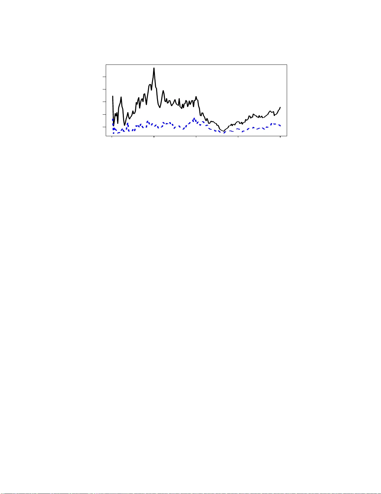
Error Bounds and Normalizing Constan ts for Sequen tial Mon te Carlo in High Dim ensions Alexandro s Beskos 1 , D an Crisan 2 , Aja y Jasra 3 , and Nick White le y 4 1 Dep artment of Statistic al Scienc e, University Col le ge L ondon, L ondon WC1E 6BT, UK . E-Mail: alex@sta ts.ucl.ac .uk 2 Dep artment of Ma thematics, Imp erial Co l le ge L ondon, L ondon, SW7 2AZ, UK . E-Mail: d.crisan @ic.ac.uk 3 Dep artment of Statistics & App lie d Pr ob ability, Nationa l University of Singap or e, Singap or e, 117546 , Sg. E-Mail: staja@nu s.edu.sg 4 Dep artment of Ma thematics, Uni versity of Bristol, Bristol, BS8 1TW, UK. E-Mail: nick.whi teley@bri stol.ac.uk Abstract In a recent pap er [3], the Sequential Monte Carlo (SMC) sampler in trod uced in [12, 19, 24] has b een shown to b e asymptotically stable in the dimension of th e state space d at a cost that is only p olynomial in d , when N the n umber of Mon te Carlo samples, is ﬁxed. More precisely , it has b een established that the eﬀective sample size (ESS) of the ensuing (app ro ximate) sample and the Mon te Carlo error of ﬁxed dimensional marginals will converg e as d grow s, with a computational cost of O ( N d 2 ). In the presen t w ork, further results on SMC methods in high dimensions are provided as d → ∞ and with N ﬁxed. W e ded uce an explicit b ound on the Monte-Carl o error for estima tes deriv ed using the SMC sampler and the exact asymptotic relative L 2 -error of the estimate of the normalizing constan t. W e also establish marginal propagatio n of chaos proper- ties of the algorithm. The accuracy in high-dimensions of some approximate SMC-based ﬁ ltering sc hemes is also discussed. Key wor ds : Sequential Mon te Carlo, H igh Dimensions, Propagation of Chaos, Normalizing Con- stants, Filtering. 1 In tro duction High-dimensional probability distributions ar e increa singly of interest in a wide v ar iety of applications. In par ticular, one is concer ne d with the estima tio n of exp ectations with resp ect to s uch distr ibutions. Due to the high-dimensional natur e of the pro bability laws, s uch integrations cannot typically b e carried out a na lytically; thus practitioner s will often reso r t to Monte Carlo metho ds. 1 2 An imp or tant Monte Car lo methodolog y is Sequen tial Monte Carlo samplers (see [1 2, 2 4]). This is a technique designed to approximate a sequence of densities deﬁned o n a common state- s pace. The metho d works by sim ulating a collectio n of N ≥ 1 weighted samples (termed par ticles) in parallel. These particles are pro pagated forward in time via Ma rko v chain Monte Carlo (MCMC), using imp or- tance sampling (IS) to c orrect, via the w eigh ts, for the discr e pancy b etw een target distr ibutions and prop osals . Due to the weigh t degeneracy problem (see e.g . [16]), resampling is adopted, sometimes per formed when the E SS drops b elow some threshold. Resa mpling generates samples with r e placement from the current co llection of par ticles using the imp or tance weigh ts, resetting un- normalized weigh ts to 1 for each sample. The ESS is a num ber b etw een 1 and N and indicates, appr oximately , the num b er of useful samples. F or SMC samplers one is t ypically interested in sa mpling a single target density on R d , but due to some complexity , a c o llection of artiﬁcial densities ar e introduced, starting at some easy to sample distribution and creating a smo oth path to the ﬁnal tar get. Recently ([2, 4, 28]) it was s hown that some IS metho ds will not stabilize, in a n appropr iate sense, as the dimension of targ et densities in a pa rticular class grows, unless N g rows exp onentially fas t with dimension d . In later work, [3] hav e established that the SMC sampler technique can be stabilize d at a cost that is only p o lynomial in d . It was s hown in [3] that E SS and the Monte Carlo erro r o f ﬁxed dimensional mar ginals stabilize a s d g rows, with a cost of O ( N d 2 ). This corres po nds to introducing d artiﬁcial densities b etw een a n initial distribution a nd the one of interest. The case of ﬁxed d a lso has bee n analyzed r ecently [30]. The ob jective of this ar ticle is to provide a mor e complete understanding of SMC alg orithms in high dimensions, complementing a nd building upon the results of [3]. A v ariety of r esults are presen ted, addressing so me gener ic theoretica l prop er ties of the algor ithms and some is sues which ar ise from sp eciﬁc cla sses of a pplication. 1.1 Problems Addressed The ﬁrst issue inv estigated is the increase in err o r of estimating ﬁxed-dimensional marg inals us ing SMC sampler s r elative to i.i.d. sampling. Considering the ca se when one resamples a t the v er y ﬁnal time-step we show that the L 2 -error inc r eases only by a facto r of O ( N − 1 ) uniformly in d . Resampling at the very ﬁnal time- s tep is o ften of imp ortance in rea l applications; see e.g. [1 4]. The s econd issue we address is the estimation of ra tios of normalizing co nstants a pproximated using SMC samplers . This is critical in ma ny disciplines , including Bay esian or cla ssical sta tistics, ph ysics and rar e event s. In particular, for Bayesian mo del comparison, Ba yes factor s are asso ciated to s tatistical mo dels in high-dimensional spaces, and these Bay es factors need to b e es tima ted by nu merical techniques such as SMC. The nor malizing cons tant in SMC metho ds has b een well-studied: see [8, 11]. Among the interesting r esults that hav e been proved in the literature is the unbiased prop erty . How e ver, to our knowledge, no re s ults hav e been prov ed in the context of asymptotics in dimension d . In this article we provide an expr ession for ﬁxed N o f the relative L 2 -error o f the SMC 3 estimate of a ratio of nor malizing co nstants. The algo rithm can include r esampling, whereby the expression diﬀers. The rate o f c o nv er gence is O ( N − 1 ), when the co mputatio nal cost is O ( N d 2 ). The results also a llow us co mpare b etw een diﬀerent seque nce s o f densities use d within the SMC metho d. The third is s ue we inv e s tigate is asymptotic indep endence prop er ties o f the particles when one resamples: pro pa gation o f chaos - see [11, Chapter 8]. This is s ue has pra ctical implications which we discuss b e low. It is shown that, in b etw een any tw o res a mpling times, any ﬁxed dimensional mar ginal distribution of a ny ﬁxed blo ck of 1 ≤ q ≤ N particles a mong the N pa rticles a r e asy mptotically independent with the correc t marg inal. This result is established as d grows with N ﬁxed, whilst the classical results require N to grow. As in [3, 3 0], this establishes that the er g o dicity o f the Mark ov kernels used in the algorithm can provide stabilit y of the algor ithm, even in high dimensions if the nu m be r o f artiﬁcial dens ities is scaled appropr ia tely with d . The ﬁna l is sue we address is the problem o f ﬁltering (s e e Se c tio n 5 for a description). Ultimately , we do no t provide a ny a nalysis of a practica l SMC a lgorithm which s tabilizes as d increases . How ever, it is shown that when one ins erts an SMC sampler in-b etw een the ar riv al of each data-p oint and up dates the entire collec tio n of states, then the alg orithm stabilizes a s d g rows at a co st which is O ( n 2 N d 2 ), n being the time parameter. This is of limited practica l use, as the co mputational stor age co sts inc r ease with n . Motiv ated by the SMC sampler r esults, we co nsider some s tr ategies which co uld b e a ttempted to stabilize hig h-dimensional SMC ﬁltering algorithms. In pa rticular, we a ddress tw o str a tegies which insert a n SMC sampler in-b etw een the a r riv al of ea ch data -p oint. The ﬁrst, which only updates the state at the curr ent time-p oint, fa ils to stabilize as the dimension grows, unless the particles increase exp onentially in the dimension. The seco nd, which us e s a margina l SMC approa ch (se e e.g. [27]) als o exhibits the same pr op erties. At presen t we are not aw are of any online (i.e. one whic h has a ﬁxed computational co st p er time step) SMC a lgorithm which can prov ably stabilize with d for any mo del , unless N is exp onential in d . It is rema rked, as noted in [4], that there exist sta tistical mo dels for which SMC metho ds c a n work quite well in hig h-dimensions. In relatio n to this, we then inv es tigate the SMC simulation of a ﬁlter based up on Approximate Bay esian Computatio n (ABC) [20]. The ABC approximation induces bias which canno t b e remo v ed in pra ctice. W e sho w here that the s imu lation error s tabilizes as the dimension grows, but we argue that the bias is likely to explo de as d g rows. This discussion is also releven t for the p o pular ensemble Kalman ﬁlter (EnK F) employed in high dimensiona l ﬁltering problems in physical sciences (e.g. [17]). The pap er is structured as follows: In Section 2 we descr ibe the SMC sa mpler algo rithm tog ether with our ma thematical assumptions. In Section 3 our main results are given. In additio n, we intro duce a gener a l annealing scheme, coupled with a consider ation of stability results fo r da ta-p oint temp ering [9]; this la tter study connects with o ur discussio n in Section 5 on ﬁltering. Section 4 consider s the practical implica tions of o ur ma in res ults with numerical simulations. The ﬁltering proble m is ad- dressed in Section 5. W e conclude with a summar y in Section 6. Most of the pro ofs o f our res ults are given in the App endix. 4 1.2 Notation Let ( E , E ) b e a measurable s pace a nd P ( E ) the set o f probability mea sures on it. F or µ a σ − ﬁnite measure on ( E , E ) and f a measura ble function, w e set µ ( f ) = R E f ( x ) µ ( dx ). F or µ ∈ P ( E ) and P a Ma rko v kernel on ( E , E ), we use the integration notation P ( f )( x ) = R E P ( x, dy ) f ( y ) a nd µP ( f ) = R E µ ( dx ) P ( f )( x ). In a ddition, P n ( f )( x ) := R E n − 1 P ( x, dx 1 ) P ( x 1 , dx 2 ) × · · · × P ( f )( x n − 1 ). The total v aria tio n diﬀerence nor m for µ, λ ∈ P ( E ) is k µ − λ k tv := sup A ∈ E | µ ( A ) − λ ( A ) | . The class of b o unded (resp. c o ntin uous and b ounded) mea surable functions f : E → R is wr itten B b ( E ) (res p. C b ( E )). F o r f ∈ B b ( E ), we write k f k ∞ := sup x ∈ R | f ( x ) | . W e will denote the L  -norm of rando m v ariables as k X k  = E 1 / | X |  with  ≥ 1. F or a g iven vector ( x 1 , . . . , x p ) a nd 1 ≤ q ≤ s ≤ p w e denote b y x q : s the sub-vector ( x q , . . . , x s ). F or a measure µ the N -fo ld pro duct is wr itten µ ⊗ N . F or a ny collection of functions ( f k ) k ≥ 1 , f k : E → R , we w r ite f 1 ⊗ · · · ⊗ f k : E k → R fo r their tensor pro duct. Throug hout M is used to denote a constant whose meaning may change, dep ending up o n the context; imp ortant depe ndencie s a r e wr itten as M ( · ). In addition, all of our re s ults hold on probability space (Ω , F , P ), with E de no ting the ex pe c tation o pe r ator and V a r the v ariance. Finally , ( ⇒ ) denotes conv ergence in distribution. 2 F ramew ork 2.1 Algorithm and Set-Up W e consider the scenar io when one wishes to sample from a tar g et distribution with density Π on E d ( E ⊆ R ) with r esp ect to Leb esg ue measure, known p oint-wise up to a nor malizing constant. In or der to sa mple from Π, we introduce a sequence of ‘bridg ing’ dens ities which start from an easy to sa mple target a nd evolv e toward Π. In particular , we will consider the densities: Π n ( x ) ∝ Π( x ) φ n , x ∈ E d , (1) for 0 ≤ φ 0 < · · · < φ n − 1 < φ n < · · · < φ p = 1 . Below, we use the short-hand Γ n to denote un- normalized dens ities asso cia ted to Π n . One ca n sample from { Π n } us ing an SMC sampler that targets the sequenc e of densities: e Π n ( x 1: n ) = Π n ( x n ) n − 1 Y j =1 L j ( x j +1 , x j ) with domain ( E d ) n of dimension that incr eases with n = 1 , . . . , p ; here, { L n } is a seq uence o f ar tiﬁcial backw ard Ma r ko v kernels that can, in pr inciple, b e arbitra rily selected ([12]). Let { K n } b e a sequence of Markov kernels of inv ariant density { Π n } a nd Υ a distr ibution; assuming the weigh ts app ea ring in the s tatement of the a lgorithm are well-deﬁned Radon Nikodym deriv atives, the SMC algor ithm we will ultimately explo re is the one deﬁned in Figur e 1. It is re ma rked that our a nalysis is not necessar ily constrained to the case of resampling accor ding to ESS. 5 0. Sample X 1 0 , . . . X N 0 i.i.d. fr om Υ and c ompute the weights for e ach p article i ∈ { 1 , . . . , N } : w i 0:0 = Γ 0 ( x i 0 ) Υ( x i 0 ) . Set n = 1 and l = 0 . 1. If n ≤ p , for e ach i sample X i n | X i n − 1 = x i n − 1 fr om K n ( x i n − 1 , · ) and c alculate the weights: w i l : n = Γ n ( x i n − 1 ) Γ n − 1 ( x i n − 1 ) w i l :( n − 1) . Calculate the Eﬀe ctive S ample Size (ESS): ESS l : n ( N ) = ( P N i =1 w i l : n ) 2 P N i =1 ( w i l : n ) 2 . (2) If ESS l : n ( N ) < a : r esample p articles ac c or ding to their n ormalise d weights w i l : n = w i l : n P N j =1 w j l : n ; (3) set l = n and r e-initialise the weights by setting w i l : n ≡ 1 , 1 ≤ i ≤ N ; let ˇ x 1 n , . . . , ˇ x N n now denote t he r esample d p articles. Set n = n + 1 . R etu rn to the start of St ep 1. Figure 1: The SMC sampler s algo rithm ana lyzed in this a r ticle. F or simplicity , we will henceforth assume that Υ ≡ Π 0 . It should b e noted tha t when Υ is diﬀerent from Π 0 , one can modify the sequence of densities to a bridging sc heme which mo v es fro m Υ to Π. How ever, in practice, o ne can make Π 0 as simple as p ossible so we do not consider this p ossibility; see [3 0] for more discuss ion a nd analysis when d is ﬁxed (note that our r e sults for SMC s amplers will hold, with some mo diﬁcatio ns, also in this scenario ). Note, that we only consider here the multinomial resampling metho d. W e will inv es tigate the stability of SMC estimates asso ciated to the alg orithm in Figure 1. T o obtain analy tica l r esults we will need to simplify the str uc tur e o f the algor ithm. In particular, we w ill consider a n i.i.d. target: Π( x ) = d Y j =1 π ( x j ) ; π ( x j ) = exp { g ( x j ) } , (4) with x j ∈ E , for s ome g : E 7→ R . In s uch a case a ll bridging dens ities are also i.i.d.: Π n ( x ) ∝ d Y j =1 π n ( x j ) ; π n ( x j ) ∝ exp { φ n g ( x j ) } . 6 It is remarked that this assumption is made for mathematical conv e nie nc e : see [3] for a dis c us sion on this. A further assumption tha t will facilitate the mathematical a na lysis is to apply indep endent kernels a long the diﬀerent co -ordinates . That is , we will as s ume: K n ( x, dx ′ ) = d Y j =1 k n ( x j , dx ′ j ) , where each trans ition kernel k n ( · , · ) pr eserves π n ( x ); that is , π n k n = π n . W e study the case when one selects co oling constants φ n = φ n ( d ) and p = p ( d ) a s b elow: p = d ; φ n (= φ n,d ) = φ 0 + n (1 − φ 0 ) d , 0 ≤ n ≤ d , (5) with 0 ≤ φ 0 < 1 giv en a nd ﬁxed with respe ct to d . It is possible, with o nly notational c hanges, to consider (as in [30]) the case when the annea ling sequence is derived v ia a mo re general non-decrea sing Lipschitz function; s ee Section 3.2.1. As in [3], it will b e conv enient to co nsider the contin uum of inv aria nt densities and kernels on the whole of the time interv al [ φ 0 , 1 ]. So, we will se t: π s ( x ) ∝ π ( x ) s = exp { s g ( x ) } , s ∈ [ φ 0 , 1 ] . Similarly k s ( x, dx ′ ) with s ∈ ( φ 0 , 1 ] is the contin uous-time version of the kernels k n ( x, dx ′ ). As in [3], the mapping l d ( s ) = ⌊ d ( s − φ 0 ) 1 − φ 0 ⌋ is used to mov e b etw een c ontin uous and discrete time. 2.2 Conditions W e state the co nditions under which w e will derive our results. W e will requir e that E ⊂ R with E b eing c omp act . The co nditions b elow co rresp ond to a simpliﬁcatio n of the weaker conditions in [3] under the scenario of the compact state space E that w e consider here. W e no te that impos ing compactness has b een done mainly to simplify pro ofs a nd keep them at a re a sonable length. The nu merical exa mples later o n are ex ecuted on unbo unded state s paces, and do not seem to in v alidate our conjecture that several o f the results in the sequel will a lso hold on unbounded spaces under appropria te geometric e r go dicity conditions, as it was the case for the stabilit y results as d → ∞ in [3]. W e rema rk that all results of [3 ] a ls o ho ld under the assumptions stated here. ( A1 ) Stability of { k s } - Uniform Er go dicity. There exists a co nstant θ ∈ (0 , 1 ) and s ome ς ∈ P ( E ) s uch that for eac h s ∈ ( φ 0 , 1 ] the state- space E is (1 , θ , ς )- s mall with r esp ect to k s . ( A2 ) Perturb ations of { k s } . There exists an M < ∞ such that for any s, t ∈ ( φ 0 , 1 ] we hav e k k s − k t k tv ≤ M | s − t | . Note that the s tatement that E is (1 , θ , ς )-small w.r .t. to k s means that E is a one-step small s et for the Marko v kernel, with minorizing distribution ς ∈ P ( E ) and parameter θ ∈ (0 , 1) (i.e. k s ( x, A ) ≥ θ ς ( A ) for each ( x, A ) ∈ E × E ). 7 In the co ntext o f our analys is, we will co nsider an SMC alg orithm that resa mples at the deterministic times t 1 ( d ) , . . . , t m ∗ ( d ) ( d ) ∈ [ φ 0 , 1 ] (i.e. res a mples after n = l d ( t k ( d )) steps for k = 1 , 2 , . . . , m ∗ ( d )) such that t 0 ( d ) = φ 0 and t 0 ( d ) < t 1 ( d ) < · · · < t m ∗ ( d ) ( d ) < t m ∗ ( d )+1 ( d ) = 1, with l d ( t m ∗ ( d )) < d . W e will als o assume that as d → ∞ we hav e that m ∗ ( d ) → m ∗ and t k ( d ) → t k for t k ∈ [ φ 0 , 1 ] for all relev ant k . Such deterministic times a re meant to mimic the b ehaviour o f randomised ones (i.e. as for the case of the original algorithm in Figure 1) and provide a ma thematically conv enien t fra mework for understanding the impact of r esampling on the pr op erties of the algor ithm. Exa mples of such times can be found in [3, 13]; the res ults therein provide an approach for co nv er ting the r esults for deterministic times, to randomized ones. In particular , they show that with a pr obability converging to 1 as N → ∞ the rando mized times essentially coincide with the deterministic ones. W e do no t consider that here as it would follow a similar pro of to [3], dep e nding up on how the resa mpling times are deﬁned. (An alternative pro cedure o f treating dynamic r esampling times is to use the co nstruction in [1]; this is no t considered here.) F or simplicity , we will henceforth as sume that d is larg e enough s o that m ∗ ( d ) ≡ m ∗ . 2.3 Log-W eigh t-Asymptotics Given the set-up (5) and the resa mpling pro cedure at the deterministic times t 1 ( d ) , . . . , t m ∗ ( d ) ∈ [ φ 0 , 1 ], and due to the i.i.d. structur e describ ed a bove, w e hav e the following expression for the pa rticle weigh ts: log( w i l d ( t k − 1 ( d )): l d ( t k ( d ) ) ) = 1 d d X j =1 ¯ G i k,j , where ¯ G i k,j = (1 − φ 0 ) P l d ( t k ( d )) − 1 n = l d ( t k − 1 ( d )) g ( X i n,j ) for 1 ≤ i ≤ N . The work in [3] illustra tes sta bilit y of the normalised weights as d → ∞ . Deﬁne the s tandardised log- weigh ts: G i k,j = (1 − φ 0 ) l d ( t k ( d )) − 1 X n = l d ( t k − 1 ( d ))  g ( X i n,j ) − E π t k − 1 ( d ) [ g ( X i n,j ) ]  . (6) The notation E π t k − 1 ( d ) [ g ( X i n,j ) ] r efers to an e x pe c tation under the initial dynamics X i l d ( t k − 1 ( d )) ,j ∼ π t k − 1 ( d ) ; after that, X i n,j will evolv e acc o rding to the Markov trans itio ns k n . W e a lso use the notation E π ⊗ N d t k − 1 ( d ) [ · ] when imp os ing s imila r initial dynamics, but now indepe ndently over all co-o rdinates and particles; such dynamics diﬀer o f c ourse fro m the actua l particle dyna mics o f the SMC algor ithm. In what follows, we use the Poisson eq uation: g ( x ) − π u ( g ) = b g u ( x ) − k u ( b g u )( x ) and in pa rticular the v aria nce s: σ 2 s : t = (1 − φ 0 ) Z t s π u ( b g 2 u − k u ( b g u ) 2 ) du , φ 0 ≤ s < t ≤ 1 . (7) The following weak limit can be derived from the pro of of Theor em 4.1 of [3]. 8 Remark 2.1 (Lo g-W eight-Asymptotics) . Assume (A 1-2) and g ∈ B b ( E ) . F or any N ≥ 1 we have:  1 d d X j =1 G i k,j  N i =1 ⇒ ( Z i ) N i =1 , wher e the Z i ’s ar e i.i.d. c opies fr om N (0 , σ 2 t k − 1 : t k ) . The result illustr a tes tha t the considera tion o f O ( d ) Markov chain steps between r esampling times stabilise the particle standar dis ed log-weights as d → ∞ . 3 Main Results W e now present the main results of the ar ticle. 3.1 Asymptotic Results as d → ∞ 3.1.1 L 2 − Error The ﬁrst res ult of the paper pertains to the Monte-Carlo er ror fro m estimates der ived via the SMC metho d. W e will consider mean squar ed e r rors a nd obtain L 2 -b ounds with resampling car ried out a lso ‘at the end’, that is when one r esamples also a t time t = 1. Below, rec a ll that the ˇ X -notatio n is for resampled par ticles. Resampling at time t = 1 is r equired when one wis hes to obtain un-weigh ted samples. W e have the following r e sult, with pro of in App endix A.2. Theorem 3. 1. Assume (A 1-2) and g ∈ B b ( E ) . Then for any N ≥ 1 , ϕ ∈ C b ( E ) we have:     1 N N X i =1  ϕ ( ˇ X i d, 1 ) − π ( ϕ )      2 2 ≤ V ar π [ ϕ ] 1 N  1 + M ( σ 2 t m ∗ − 1 :1 )  for M ( σ 2 t m ∗ − 1 :1 ) = e σ 2 t m ∗ − 1 :1 + M e 17 σ 2 t m ∗ − 1 :1 1 N 1 / 6 with M < ∞ indep endent of N and σ 2 t m ∗ − 1 :1 . Remark 3. 1. Co mp ar e d to the i.i.d. sampling sc enario, the upp er b ound c ontains the additional term V ar π [ ϕ ] 1 N M ( σ 2 t m ∗ − 1 :1 ) . This is a b ound on the c ost induc e d due to the dep endenc e of the p articles. 3.1.2 Normalizing Constan ts The se cond main result o f the pa per is the stability of es timating norma lising cons tants in high dimen- sions. The quantit y of interest her e is the ratio o f normalising constants: c d := R E d Π( x ) dx R E d Π φ 0 ( x ) dx . (8) 9 W e ﬁrst consider the SMC sampler in Figur e 1 with no resampling. Deﬁne: γ N d (1) = 1 N N X i =1 w i 0: d ≡ 1 N N X i =1 e 1 d P d j =1 ¯ G i j ; γ d (1) = E  e 1 d P d j =1 ¯ G 1 j  , where ¯ G i j = (1 − φ 0 ) P d − 1 n =0 g ( X i n,j ). F r om standard prop erties of SMC we hav e E [ γ N d (1) ] = γ d (1) ≡ c d . Now, co nsider the re lative L 2 -error : V 2 ( γ d (1)) = E   γ N d (1) γ d (1) − 1  2  . W e then hav e the following result, proven in App endix A.3. Theorem 3. 2. Assume (A 1-2) and g ∈ B b ( E ) . Then for any N ≥ 1 : lim d →∞ V 2 ( γ d (1)) = e σ 2 φ 0 :1 − 1 N . The result establis he s a O ( N − 1 ) r ate of con v ergence at a computational cost of O ( N d 2 ). The infor- mation in the limit is in terms of the expr ession σ 2 φ 0 :1 . As in [3], this is a critical quantit y , which helps to mea s ure the rate of c o nv er gence of the algo rithm. W e now co nsider the SMC sampler in Figur e 1 with resa mpling at the deterministic times { t k ( d ) } describ ed in Section 2.2. W e make the following deﬁnitions: γ N d,k (1) = 1 N N X i =1 e 1 d P d j =1 ¯ G i k,j ; γ d,k (1) = E π ⊗ N d t k − 1 ( d )  e 1 d P d j =1 ¯ G 1 k,j  , where k ∈ { 1 , . . . , m ∗ + 1 } and ¯ G i k,j as deﬁned in Sec tio n 2.3. As in the non-r esampling ca se, we a gain hav e the unbiasedness prop erty for the es tima te of c d : E  Q m ∗ +1 k =1 γ N d,k (1)  = Q m ∗ +1 k =1 γ d,k (1) ≡ c d . W e hav e the following result whose pro o f is in App endix A.3 . Theorem 3. 3. Assume (A 1-2) and g ∈ B b ( E ) . Then for any N ≥ 1 : lim d →∞ V 2  m ∗ +1 Y k =1 γ d,k (1)  = e − σ 2 φ 0 :1 m ∗ +1 Y k =1  1 N e 2 σ 2 t k − 1 : t k +  1 − 1 N  e σ 2 t k − 1 : t k  − 1 . Remark 3 .2. In c omp arison with the no r esampli ng sc enario, t he limiting expr ession her e dep ends up on the incr ement al varianc e expr essions. On writing the limit in the form: e − σ 2 φ 0 :1 m ∗ +1 Y k =1 e σ 2 t k − 1 : t k  1 + 1 N { e σ 2 t k − 1 : t k − 1 }  − 1 if N > ( m ∗ + 1 )( e σ 2 − 1 ) , with σ 2 = ma x k σ 2 t k − 1 : t k , t hen using similar manipulations to [8, Cor ol lary 5.2], we have that lim d →∞ V 2  m ∗ +1 Y k =1 γ d,k (1)  ≤ 2( m ∗ + 1 )( e σ 2 − 1 ) N henc e, the no r esampling s c enario has a lower err or if this is less than the limit in The or em 3.2. The upp er-b ound also shows that the err or se ems to gr ow with numb er of t imes one r esamples. The limit in 10 The or em 3.3 c orr esp onds to t he b ehavio r of E π ⊗ N d t k − 1 ( d ) [ γ N d,k (1) 2 /γ d,k (1) 2 ] b etwe en e ach r esampling t ime. In eﬀe ct, the er go dicity of the system takes over, and br e aks up the err or in estimation of the r atio of normalizing c onstant s to diﬀer ent t ours b etwe en r esampling t imes (s e e Pr op osition 3.1). T o provide so me intuit ion for Theo rem 3.3, we give the fo llowing result. It is asso c iated to the asymptotic indep endence, b etw een re s ampling times, of the lo g -weigh ts P d j =1 1 d G i k,j in (6). The pro of of the following can b e found in App e ndix A.3. Prop ositi on 3.1. Assume ( A 1-2) and that g ∈ B b ( E ) . Then for any N ≥ 1 , i ∈ { 1 , . . . , N } , c 1: k ∈ R and k ∈ { 1 , . . . , m ∗ + 1 } , we ha ve t hat: lim d →∞ E  e P k l =1 c l 1 d P d j =1 G i l,j  = k Y l =1 E [ e c l Z l ] , wher e Z l ∼ N (0 , σ 2 t l − 1 : t l ) indep endently over 1 ≤ l ≤ k . 3.1.3 Propagation of Chaos Finally w e deduce a r ather classical result in the analysis of par ticle systems: propaga tion of c haos, demonstrating the asymptotic (in the class ical setting) indep endence of a ny ﬁxed blo ck of q of N particles as N grows. The following scena rio, with the SMC sampler with resampling (at the times { t k ( d ) } ), is considered: let s ( d ) be a s e quence such that s ( d ) ∈ ( t k − 1 ( d ) , t k ( d )) for so me 1 ≤ k ≤ m ∗ + 1, with limit s ∈ ( t k − 1 ( d ) , t k ( d )). Denote by P ( q,N ) s ( d ) ,j the marg inal law o f a ny o f the q particles out of N at time s ( d ) and in dimension j ∈ { 1 , . . . , d } . B y constructio n, pa rticles are considere d at a time when they ar e not resampled. W e hav e the follo wing Propa gation of Cha os result, whose pro of is in Appendix A.4. Prop ositi on 3. 2. Assu me (A1-2) and that g ∈ B b ( E ) . Then, for any ﬁxe d j ∈ { 1 , . . . , d } and any 1 ≤ k ≤ m ∗ + 1 , a se qu enc e s ( d ) ∈ ( t k − 1 ( d ) , t k ( d )) with s ( d ) → s , and any N ≥ 1 , with 1 ≤ q ≤ N ﬁxe d: lim d →∞ k P ( q,N ) s ( d ) ,j − π ⊗ q s k tv = 0 . The result establishes the asy mptotic indep endence of the marginals of the particle s , b etw een any t wo resampling times, a s d grows. This is in contrast to the standar d s c enario where the par ticles only bec ome indep endent as N gr ows. Critically , the MCMC s teps provide the eﬀect that the marg inal particle distributions conv erge to the target π ⊗ q s . Thus, Pr op osition 3.2 esta blishes that it is essentially the ergo dicity o f the system which helps to driv e the stabilit y pr op erties of the algorithm. It should be noted that if o ne considers the pa rticles just after res ampling, one cannot obtain an as y mptotic independenc e in d . Here, a s in clas sical results for particles metho ds, one ha s to rely on increasing N . 11 3.2 Other Sequences of D ensities In this section, we discus s so me iss ues a sso ciated w ith the selectio n of the sequence of chosen bridging densities { Π n } . 3.2.1 Annealing Sequence Recall that we use the equidista n t annealing sequence φ n in (5). Ho wev er , one could also consider a general diﬀerentiable, increa s ing Lipschitz function φ ( s ), s ∈ [0 , 1] with φ (0) = φ 0 ≥ 0 , φ (1) = 1, and use the co nstruction φ n,d = φ ( n/d ); then the a symptotic result in Theorem 2.1 (and others that will follow) g eneralised to the choice of φ n,d considered here would inv olv e the v ar iances: σ 2 ,φ s : t = Z t s π φ ( u ) ( b g 2 φ ( u ) − k φ ( u ) ( b g φ ( u ) ) 2 )  dφ ( u ) du  dφ ( u ) , 0 ≤ s < t ≤ 1 , (9) in the place of σ 2 s : t in (7). Our pr o ofs in this pap er are g iven in terms of the annealing s e quence (5), corres p o nding to a linea r choice o f φ ( · ), but it is stra ightforw ard to mo dify them to the a b ove scena rio. This p oint is illuminated by our main results. F or exa mple Theo rem 3 .2 he lps to compare v ar ious annealing schemes fo r estimating normalizing consta nt s, via the limiting qua ntit y (9). That is , if we ar e only concerned with v ar iance one prefers an annealing scheme which dis cretizes φ ( s ) versus one which discretizes ν ( s ) (diﬀerentiable monotonic incre a sing Lipschitz function with ν (0) = ν 0 > 0 , ν (1) = 1 ) for estimating normalizing constants if e σ 2 ,φ 0:1 − 1 N ≤ e σ 2 ,ν 0:1 − 1 N ⇐ ⇒ σ 2 ,φ 0:1 ≤ σ 2 ,ν 0:1 . In practice, how ever, one has to num erically approximate σ 2 ,φ 0:1 and σ 2 ,ν 0:1 , less ening the practical impact of this r esult. Similar to the scenar io of Theorem 3.2, one can use Theorem 3.3 to compar e annealing schemes φ ( s ) a nd ν ( s ) (which p otentially generate a diﬀerent collection and num b er of limiting times 0 < t φ 1 < · · · < t φ m ∗ φ ≤ 1, m ∗ φ and 0 < t ν 1 < · · · < t ν m ∗ ν ≤ 1, m ∗ ν resp ectively) via the inequality e − σ 2 ,φ 0:1 m ∗ φ +1 Y k =1 h 1 N e 2 σ 2 ,φ t φ k − 1 : t φ k + N − 1 N e σ 2 ,φ t φ k − 1 : t φ k i ≤ e − σ 2 ,ν 0:1 m ∗ ν +1 Y k =1 h 1 N e 2 σ 2 ,ν t ν k − 1 : t ν k + N − 1 N e σ 2 ,ν t ν k − 1 : t ν k i but a gain, b oth qua ntit ies are diﬃcult to calculate. 3.2.2 Data P oint T emp ering An int eresting sequence of densities intro duced in [9] arises in the scena rio when Π is asso cia ted with a batch data-set y 1 , . . . , y p . The idea is to constr uct the sequence of densities so that a r riving data - p o ints are added sequentially to the ta r get as the time parameter o f the algo rithm increas es. More co ncretely , we will a ssume here that: Π( x ) ∝ exp  p X k =1 d X j =1 g ( y k , x j )  , x j ∈ E , 12 that is a dens it y that is i.i.d. in b oth the data a nd dimension. In this scena r io one could then adopt a sequence of densities of the form: Π n ( x ) ∝ ex p  n X k =1 d X j =1 g ( y k , x j )  , 1 ≤ n ≤ p . As noted also in Remark 3.5 of [3], fo r d → ∞ one cannot sta bilize the asso ciated SMC algor ithm (describ ed in Figure 1) a s the ra tio Π n +1 / Π n explo des for increasing d . T o sta bilize the a lgorithm as d gr ows one can insert ⌊ d/p ⌋ annealing steps betw een consecutive data p oints, thus forming the densities: Π ( n ) k ( x ) ∝ exp  φ  k ⌊ d/p ⌋  d X j =1 g ( y n , x j )  × Π n − 1 ( x ) , n ∈ { 1 , . . . , p } , k ∈ { 1 , . . . , ⌊ d p ⌋} , where φ ( s ) is as in Section 3 .2.1 with φ 0 = 0. Then o ne can adopt Markov kernels K ( n ) s , 1 ≤ n ≤ p , of pro duct for m with each comp one nt kernel k ( n ) s having inv ariant measure π ( n ) s ( x ) ∝ exp  s · g ( y n , x ) + n − 1 X k =1 g ( y k , x )  , x ∈ E . W e conside r the scenario where there is no r esampling and denote by E SS (0 ,d ) ( n, N ) the eﬀective sample size with n data after ⌊ d/ p ⌋ steps of the n -th SMC sa mpler. Throughout the data are taken as ﬁxed. W e hav e the following result, which follows dir ectly fr o m Theorem 3 .1. of [3] and illustrates the stability of ESS (0 ,d ) ( n, N ) as d → ∞ . Prop ositi on 3.3. Assume c onditions (A1-2) for the kernels k ( n ) s , n ∈ { 1 , . . . , p } . Supp ose that for e ach data index n ∈ { 1 , . . . , p } , g ( y n , · ) ∈ B b ( E ) . Then, for any ﬁxe d N > 1 and n ≥ 1 , ESS (0 ,d ) ( n, N ) c onver ges in d istribution to:  P N i =1 e Z i  2 P N i =1 e 2 Z i wher e Z i i.i.d. ∼ N (0 , σ 2 ) with σ 2 = n X k =1 Z 1 0 π ( k ) φ ( u ) (( b g ( k ) φ ( u ) ) 2 − k ( k ) φ ( u ) ( b g ( k ) φ ( u ) ) 2 )  dφ ( u ) du  dφ ( u ) . In p articular, lim d →∞ E  ESS (0 ,d ) ( n, N )  = E   P N i =1 e Z i  2 P N i =1 e 2 Z i  . As for the case with annealing densities, there is a direct e x tension to the ca se wher e one resamples (see [3]). In addition, one can ea sily extend the results in Sectio n 3 in the data -p oint temp ering case examined here. In connection to the ﬁltering scenario, this is a class of densities that falls into the scenario of a sta te-space mo del with a deter ministic dynamic on the hidden state (i.e. only the initial state is sto chastic and propa g ated deterministica lly; see e.g . [7]). This hints at algor ithms for ﬁltering which may sta biliz e as the dimensio n gr ows. As we shall see in Sectio n 5, it is not straight-forward to do this. 13 4 Numerical Sim ulations W e now present tw o numerical ex a mples, to illustrate the pr actical implications of our theoretica l results. It is noted that the s tate-space E is not compact her e, yet the impact of our re s ults can still be observed. 4.1 Comparison of Annealing Scheme s W e consider a ta r get distribution comprised o f d i.i.d. N (0 , 1) co-ordina tes. The bridg ing densities are in this ca se: π φ ( s ) ( x ) ∝ exp  − 1 2 φ ( s ) x 2  . (10) W e will in fact consider tw o annealing schemes: φ ( s ) = φ 0 + (1 − φ 0 ) s ; ν ( s ) = φ 0 e ϑ − 1 e ϑ − 1 +  1 − φ 0 e ϑ − 1  e ϑs . (11) These a re graphica lly displayed in Figure 2 (a), with ϑ = 5. The purp ose of investigating the t w o annea ling schemes is as follows. In practica l applica tions o f SMC samplers we hav e observed tha t algorithms with slo w initial annea ling schemes can often o ut- per form those with faster ones (see Figure 2 (a)). Thus, we expect scheme ν ( s ) to p erfor m b etter than φ ( s ) w.r.t. the express ion for the asymptotic v a riance (9), hence deliver a low er rela tive L 2 - error for the estimatio n of the no r malizing co nstant in hig h dimensions. T o o btain some analytically computable proxies for the asymptotic v ar iances (9) we use the v ar ia nces that o ne would obtain when k s ( x, dx ′ ) ≡ π s ( dx ′ ), that is we substitute π φ ( u ) ( g 2 ) − π φ ( u ) ( g ) 2 for π φ ( u ) ( b g 2 φ ( u ) − k φ ( u ) ( b g φ ( u ) ) 2 ) in (9). In this sce nario it is simple to show that, under the choice (10), we hav e that: σ 2 ,φ 0:1 = 1 2 Z 1 0  1 φ ( u ) dφ ( u ) du  2 du . Figure 2 (b) now plots the analytically av ailable v ariances σ 2 ,φ 0:1 and σ 2 ,ν 0:1 (broken line) aga inst φ 0 . The graph indeed provides some evidence that that the scheme ν ( s ) sho uld give b etter results. This is particularly eviden t when φ 0 is small; this is unsur pr ising as one initia lizes from Π φ 0 , hence if φ 0 is closer to 1 o ne exp ects a constant incr ease in the a nnealing par ameter to b e pr e ferable to a slow initial evolution. W e ran SMC samplers with b oth annea ling schemes with N = 1 0 4 particles and diﬀer ent dimensio n v alues d ∈ { 10 , 2 5 , 50 } . The c hoice φ 0 = 1 d is used for both annealing schemes. W e used a Marko v kernel k s ( x, dx ′ ) cor resp onding to a Rando m- W alk Metrop olis with pro p o sal y = x + N (0 , 1 25 φ 0 ), thus the pro p osal v ar iance is 1 / 25 times the v ar iance o f the starting distribution of the br idg e N (0 , 1 φ 0 ); this is a choice that g av e go od acceptance probabilities ov er all d bridging steps of the sa mpler. Multinomial resampling was used when the eﬀective sample size dropp ed b elow N 2 . W e made 50 indep endent runs 14 Dimension d 10 25 50 Ratio of V aria nces (for φ ( s ) over ν ( s )) 2.32 3.47 7.05 T able 1: The empirical v a r iances (o v en 50 indep endent runs for the SMC sampler) of the log Ratio (12) us ing the a nnealing φ ( s ) ov e r the cor resp onding v ariances for the a nnealing sequence ν ( s ). 0 20 40 60 80 100 0.0 0.2 0.4 0.6 0.8 1.0 s annealing parameter (a) Annealing Sc hemes, φ 0 = 0 . 01 0.00 0.01 0.02 0.03 0.04 0.05 0 100 200 300 400 500 φ 0 asymptotic variance (b) Asymptotic V ari ances Figure 2: Panel (a): Plot of the a nnealing para meters φ ( s ) and ν ( s ) (broken line) deﬁned in (11) against time when φ 0 = 0 . 01 and ϑ = 5. Panel (b): A Plot of σ 2 ,φ 0:1 and σ 2 ,ν 0:1 (broken line) against φ 0 for the case of e xact s ampling with k s ( x, dx ′ ) ≡ π s ( dx ′ ) and the s cenario (10). of the a lgorithm, and c alculated the corre s p o nding rea lis ations of the log Ratio: m ∗ ( d )+1 X k =1 log  γ N d,k (1) γ N d,k − 1 (1)  log  γ d,k (1) γ d,k − 1 (1)  (12) (note that now the re s ampling times and their num ber ar e ra ndom) and their sa mple v a riance. This exp eriment was ca rried out for choices of dimensio n d ∈ { 1 0 , 25 , 50 } and for both annealing schemes φ ( s ) and ν ( s ). The ra tio of the obtained v a riances for the a nnealing sequence φ ( s ) over ν ( s ) a re shown in T able 1. The results co nﬁrm our theoretical ﬁndings ab ov e for the sup er iority of ν ( s ) over φ ( s ) based on the a nalytical express ion for the asymptotic v a riance even for mo der ate d . 4.2 Ba y esian Linear Mo del W e now consider the implica tions of main r esults in the context of a B ayesian linear regr ession mo del (see [15] for a b o ok- length int ro duction as well a s a wealth of pra ctical applications ). This is a statistical mo del that asso ciates a p -vector of re sp onses, say Y , to a p × d -matrix of expla natory v ariables, X , 15 Time-Steps d 5 d 10 d Relative Erro r 4.75 4.4 7 3.9 T able 2 : The mean squar e er ror when estimating E [ β 1 | Y ] for the (annealed) SMC sampler ov er 1 00 rep eatitions r e lative to i.i.d. sampling. 100 0 particles a r e run and we resample at the ﬁna l time step. The er ror is ca lc ulated for diﬀerent choices of num ber of time-steps for the SMC sa mpler. for some p ≥ 1, d ≥ 1. In par ticular: Y = X β + ǫ where β is a d - vector of unknown reg ression c o eﬃcients a nd ǫ ∼ N p (0 , 1 p ), with 1 p the p × p identit y matrix. A prior dens it y on β is tak en as N d (0 , 1 d ) which yields a p osterio r density found to be the d -dimensional Gaussian N d (( 1 d + X ′ X ) − 1 X ′ Y , ( 1 d + X ′ X ) − 1 ) where X ′ denotes transpo se. This is the target distr ibution for our SMC sampler . The ob jective is to inv estig ate the b ound in Theor em 3 .1 and the implications of Pro p osition 3.2. Note that the ta r get distribution is not of pro duct structure here. The data-p oint temp ering metho d (see Section 3.2.2) is a lso compar e d with annealing. W e consider the cas e d = 50, p = 50 with N = 10 3 ; the data a r e all simulated. The annealing scheme ν in (11 ) is ado pted as well a s the data-p o int temper ing metho d with ⌊ 10 d/p ⌋ steps b etw een the p data point a rriv a ls. Particles are propag ated along the bridging densities via Marko v kernels co r resp onding to Random-W a lk Metrop olis within Gibbs: the prop osa l for a univ a r iate co-or dinate x conditiona lly on the rest is y = x + N (0 , 1 16 ). Dynamic r esampling according to the ESS is employ ed (threshold N 2 ) as well as resa mpling a t the last time step (see Theore m 3 .1). F o r the annealing scheme the n umber of SMC s teps is s caled a s a m ultiple of d ). This increas e at the num ber of time steps aims at illustr ating the propag ation of chaos (Prop ositio n 3.2). W e ﬁxed d = 50 for computationa l cos t considerations, but the SMC algorithms will eas ily s ta bilize for muc h larg er d . Each SMC metho d e mployed is rep eatedly applied 100 times. W e calculate the mea n squa re err or for the estimation of E [ β 1 | Y ] (analytically av ailable here) ov er the 100 replications and we co mpare with the corres po nding erro r under i.i.d. sampling of the p o s terior of β 1 ; the results a re r ep orted in T able 2. In the table we ca n observe the incr ease in mean squar e error of the (annealed) SMC algo r ithm to i.i.d. simulation. The increase here is not substan tial a s indicated by Theo rem 3 .1, although one may need to take d very larg e (and hav e a n i.i.d. tar get) b efore the b ound in Theorem 3 .1 is realized. As the num b er of time-steps incr eases we ca n observe an improvemen t. This is due to increase in diversit y of the p opulation, which improv es the SMC estimate even when r esampling at the end. F or the data-p oint tempering metho d (the CP U time is ro ughly comparable with the case of 10 d time- steps o f the annealed SMC) the co rresp onding v alue o f the relative mean squar e er r or is 7.5, which is slightly worse than the annealing sc heme. In general, it is diﬃcult to draw a deﬁnite conclusion on which scheme may b e b etter. 16 5 Filtering An imp or tant applica tion o f SMC methods is ﬁltering . In the following we will loo k at the eﬀect of dimension fo r s e veral ﬁlter ing a lgorithms. 5.1 Set-Up Consider the dis crete-time ﬁltering pro blem; we hav e ﬁxed obser v ations y 1 , . . . , y n , with y k ∈ R d y and a hidden Markov chain X 1 , . . . , X n , with X k ∈ E d such that the Y k ’s a re conditionally indep endent o f all o ther v ariables, g iven X k . W e a ssume that the density w.r .t. Leb esgue measure is g ( y k | x k ) = exp  d X j =1 h ( y k , x k,j )  (13) with x k,j ∈ E and h : R d y × E → R . The hidden Markov chain is ta ken to b e time-homoge neo us w ith transition density w.r.t. Leb esgue measur e: F ( x k | x k − 1 ) = d Y j =1 f ( x k,j | x k − 1 ,j ) , k ≥ 1 , where x 0 = ( x 0 , 1 , x 0 , 2 , . . . , x 0 ,d ) ∈ E d is a given ﬁxed p oint and R E f ( x ′ | x ) dx ′ = 1. This is certainly a very sp eciﬁc mo del structure chosen, as in the pr e vious part o f the pap er, for mathematical convenience. Clearly , our res ults dep end on the giv en str ucture; it is cer ta inly the case tha t for some o ther c la sses of state- space mo dels standard SMC metho ds could stabilize with the dimensio n of the pr oblem (as could b e the case for instance when the liheliho o d in (13 ) inv o lved only a few of the co-or dinates of x ). The ob jective in ﬁltering is to compute for a π -integrable function ϕ : E [ ϕ ( X n ) | y 1: n ] = Z E ϕ ( x ) π n ( x n | y 1: n ) dx n (14) where π n ( x n | y 1: n ) = R E ( n − 1) d Q n k =1 g ( y k | x k ) F ( x k | x k − 1 ) dx 1: n − 1 R E nd Q n k =1 g ( y k | x k ) F ( x k | x k − 1 ) dx 1: n . It should b e noted that o ne can re-wr ite the ﬁlter via the standa r d pr ediction-up dating formula: π n ( x n | y 1: n ) = g ( y n | x n ) π n | n − 1 ( x n | y 1: n − 1 ) p ( y n | y 1: n − 1 ) ; π n | n − 1 ( x n | y 1: n − 1 ) = Z E d F ( x n | x n − 1 ) π n − 1 ( x n − 1 | y 1: n − 1 ) dx n − 1 ; p ( y n | y 1: n − 1 ) = R E nd Q n k =1 g ( y k | x k ) F ( x k | x k − 1 ) dx 1: n R E ( n − 1) d Q n − 1 k =1 g ( y k | x k ) F ( x k | x k − 1 ) dx 1: n − 1 . Typically , one cannot calcula te (14), so we reso rt to particle ﬁltering. The most ba sic a pproach is to p erfo rm a n SMC a lg orithm, which a pproximates the sequence of densities π ( x 1: n | y 1: n ) ∝ n Y k =1 g ( y k | x k ) F ( x k | x k − 1 ) 17 by using the prio r dynamics, c haracterise d by F , as a pro p o sal. This yie lds an un-normalized incre- men tal weight at time s tep n o f the a lgorithm which is g ( y n | x n ). One can then resample or not. W e consider the scenario as the dimension of the state increases , when the data record is ﬁxed (i.e. we keep the time parameter n a nd data ﬁxed). In reference to the w orks [2 , 4, 6, 28], it is clear that the standar d par ticle ﬁlter canno t b e used in general to approximate ﬁlters with hig h-dimensional states. An alternative, as men tioned for the data-p oint temp ering scenario in Section 3.2.2 (see also [4, 18]) is to inser t a n annea ling SMC sa mpler betw een co nsecutive ﬁltering steps, up dating the entire tra jectory x 1: n ∈ E nd . Assuming the i.i.d. structur e ab ove, the mo del dyna mics deco mpo se over d indep endent co-or dinates. One c ould use MCMC kernels for the SMC sampler s b etw e en arriv als of consecutive data-p o int s, with each univ a riate kernel (the pro duct of d of them for ming the co mplete kernel) having inv ariant density: π ( n ) p ( x 1: n ) ∝ exp n φ  p d  h ( y n , x n ) + log ( f ( x n | x n − 1 )) + n − 1 X i =1 { h ( y i , x i ) + log ( f ( x i | x i − 1 )) } o , for x 1: n ∈ E n , φ (0) = 0 , a nd 0 ≤ p ≤ d . W e write these margina l tar get densities at data-time n on the contin uum as π ( n ) s with asso ciated Mar kov kernels k ( n ) s (whic h op erate on spa ces of incre asing dimension). No r esampling is a dded to the algor ithm, but eas ily c o uld b e. The ESS (se e (2) in Figure 1) is denoted ESS (0 ,d ) ( n, N ). It is a str aight-forward applica tion of Theo rem 3.1 of [3] to get that, under ass umptions (A1-2) for the kernels k ( n ) s , n ≥ 1, and the condition that for eac h n ≥ 1, h ( y n ; x n ) ∈ B b ( E ) (with the asso ciated solution to Poisson’s equation written ˆ g ( n ) s ), for any ﬁxed N > 1, n ≥ 1, ESS (0 ,d ) ( n, N ) converges in distribution to [ P N i =1 e Z i ] 2 P N i =1 e 2 Z i where Z i i.i.d. ∼ N (0 , σ 2 ) with σ 2 = n X k =1 Z 1 0 π ( k ) φ ( u ) (( ˆ g ( k ) φ ( u ) ) 2 − k ( k ) φ ( u ) ( ˆ g ( k ) φ ( u ) ) 2 )  dφ ( u ) du  dφ ( u ) . In par ticular, lim d →∞ E  ESS (0 ,d ) ( n, N )  = E  [ P N i =1 e Z i ] 2 P N i =1 e 2 Z i  . (15) Thu s the cos t for this alg orithm to b e stable as d → ∞ , is O ( n 2 d 2 N ). This result is not surprising; one upda tes the whole state-tra jector y and the stability prov ed in [3] is easily imp orted into the alg orithm. How ever, this algor ithm is not online and will b e of limited practica l signiﬁcance unless one has ac cess to s ubstantial computational p ow er. The result is also slightly misleading: it a ssumes that the MCMC kernels hav e a unifor m mixing with resp ect to the time parameter of the HMM (see condition A1). This is unlikely to hold unless one incr eases the computational eﬀort, ass o ciated to the MCMC kernel, with n . 18 One apparent gener a lization would b e to use SMC samplers at each data- p o int time to sample from the a nnealed smo othing densities, except freezing the ﬁrst n − 1 co-o rdinates; it is then easily seen that one do es not hav e to store the tra jectory . How ever, one can use the follo wing intuition as to why this pro cedure w ill not w ork well (the follo wing is based up on per sonal comm unication with Prof. A. Doucet). In the idealized scenario, o ne samples exactly from the ﬁnal target density of the SMC sampler . In this case, the ﬁnal target dens it y is exactly the conditionally optimal pr op osal (se e [16]) and the incr emental weigh t is: Z E d g ( y n | x n ) F ( x n | x n − 1 ) dx n = d Y j =1 Z E e h ( y n ,x n,j ) f ( x n,j | x n − 1 ,j ) dx n,j , which will typically hav e exp onentially increasing v ar iance in d . W e conjecture that similar issues arise for adv anced SMC appro aches such as [10]. 5.2 Marginal Algor ithm Due to the obvious instability of the ab ov e pro cedure, we co nsider another alterna tive, pr esented e.g . in [27]. This algorithm would pro ceed as follows. When ta rgeting the ﬁlter a t time 1, one adopts an SMC sampler, which as discussed b efore, will stabilize with the dimension. Then at subsequent time-steps, to consider the initial density of the SMC sampler : N X l =1 w l, ( n − 1) d d Y j =1 f ( x l ′ , ( n ) 0 ,j | x l, ( n − 1) d,j ) (16) where we have deﬁned: w l, ( n − 1) 0: d − 1 ∝ exp n 1 d d X j =1 d − 1 X i =0 h ( y n − 1 , x l, ( n − 1) i,j ) o ; N X l =1 w l, ( n − 1) d = 1 , as the normaliz ed weigh t. One could then resample a nd a pply SMC sampler s on the sequence o f tar get distributions (e.g. with n = 2 ) π ( n ) k ( x 1: d ) ∝ exp n φ  k d  d X j =1 h ( y n , x j ) oh N X l =1 d Y j =1 f ( x j | ˇ x l, ( n − 1) d,j ) i , k ∈ { 0 , . . . , d } , (17) where ˇ x l, ( n − 1) d,j is the r esampled particle when sampling from (16). Using simple intuition, one might exp ect that this SMC algo r ithm may stabilize as the dimension grows. F or example, if o ne co uld sample exactly from π ( d ) p ( x 1: d ), then the imp or tance weigh t is exactly 1; there is no weigh t degenera cy problem: As proved in [3], under ergo dicity assumptions, the SMC sampler will a symptotically pro duce a sample from the ﬁnal tar g et density . How ever, the following re s ult s uggests that the algo rithm will colla ps e unless the num b er of particles grows exp onentially fast with the dimension. Consider the case with N d particles, where N dep ends on d here, a nd these are sa mples exactly from the prev ious ﬁlter; denote the s a mples ˇ X 1: N d 1: d . Conditiona lly 19 upo n ˇ X 1: N d 1: d , s ample X 1: N d 1: d exactly from the approximation π ( n ) d (17). This pr esents the mo st optimistic scenario one could ho p e for. Denote b elow, ϕ n ( x ) = ϕ ( x ) − π n ( ϕ ). W e have the following r esult. Prop ositi on 5. 1. Consider the algorithm ab ove so that for any ( x, x ′ ) ∈ E 2 we have f ( x | x ′ ) ∈ ( f , f ) for c onstants 0 < f < f < ∞ and for any ( y , x ) ∈ R d y × E , h ( y | x ) ∈ ( h , h ) for 0 < h < h < ∞ . Supp ose ϕ ∈ B b ( E ) . Then, ther e exist an M < ∞ and κ > 1 such that for any d ≥ 2 , j ∈ { 1 , . . . , d } and N d ≥ 1 we have E h  1 N d N d X i =1 ϕ n ( X i j )  2 i ≤ M κ d N d . Pr o of. Throug hout the pro of, write π ( n ) d as the a pproximated ﬁlter at time n . Then we hav e the simple decomp osition: E h  1 N d N d X i =1 ϕ ( X i j ) − π n ( ϕ )  2 i = E h  1 N d N d X i =1 ϕ ( X i j ) − π ( n ) d ( ϕ ) + π ( n ) d ( ϕ ) − π n ( ϕ )  2 i . On a pplying the C 2 − inequality , we c a n decomp ose the err or into the one of the Monte Car lo error o f approximating exp ecta tions w.r.t. π ( n ) d and that of approximating the ﬁlter. Consider the ﬁrst erro r. Conditioning on the i.i.d. samples drawn from the ﬁlter at time n − 1, one may a pply the Mar cinkiewicz-Zyg mund inequa lity and use the i.i.d. prop er t y o f the a lgorithm to obtain the upper b ound:  M N d  E  1 N d P N d i =1 f ( ϕ 2 e h )( ˇ X i j ) Q l 6 = j f ( e h )( ˇ X i l ) 1 N d P N d i =1 Q d l =1 f ( e h )( ˇ X i l ) −  1 N d P N d i =1 f ( ϕe h )( ˇ X i j ) Q l 6 = j f ( e h )( ˇ X i l ) 1 N d P N d i =1 Q d l =1 f ( e h )( ˇ X i l )  2  . As ϕ and h a re b ounded, it is easily seen tha t the function in the exp ectation is uniformly b ounded in d and hence that o ne has an upper -b ound of the form M / N d . Now to deal with the second erro r, this can b e written: E   1 N d P N d i =1 f ( ϕe h )( ˇ X i j ) Q l 6 = j f ( e h )( ˇ X i l ) 1 N d P N d i =1 Q d l =1 f ( e h )( ˇ X i l ) − π n − 1 f ( ϕe h ) π n − 1 f ( e h ) d − 1 π n − 1 f ( e h ) d  2  . The bra ck e t can b e decomp os e d into the form:  1 N d P N d i =1 f ( ϕe h )( ˇ X i j ) Q l 6 = j f ( e h )( ˇ X i l ) { π n − 1 f ( e h ) d } 1 N d P N d i =1 Q d l =1 f ( e h )( ˇ X i l )  π n − 1 f ( e h ) d − 1 N d N d X i =1 d Y l =1 f ( e h )( ˇ X i l )  + 1 π n − 1 f ( e h ) d  1 N d N d X i =1 f ( ϕe h )( ˇ X i j ) Y l 6 = j f ( e h )( ˇ X i l ) − π n − 1 f ( ϕe h ) π n − 1 f ( e h ) d − 1  . Applying the C 2 − inequality a g ain, we can break up the tw o ter ms. Using the low er b ound on h and upper -b ounds on ϕ a nd h the L 2 -error o f the ﬁrst term is upp e r-b ounded by: k ϕ k 2 ∞ e 2 h π n − 1 f ( e h ) 2 d e 2 h E   π n − 1 f ( e h ) d − 1 N d N d X i =1 d Y l =1 f ( e h )( ˇ X i l )  2  = k ϕ k 2 ∞ e 2 h N d π n − 1 f ( e h ) 2 d e 2 h V ar h d Y l =1 f ( e h )( ˇ X 1 l ) i . 20 As the v a riance on the R.H.S. is easily seen to b e equal to π n − 1 ( f ( e h ) 2 d ) − π n − 1 ( f ( e h )) 2 d one yields the upper -b ound: M N d  π n − 1 ( f ( e h ) 2 d ) π n − 1 ( f ( e h )) 2 d − 1  . F or the seco nd term one can follow similar arg uments to yield the upp er -b ound: 1 N d π n − 1 [ f ( e h )] 2 d h π n − 1 [ f ( ϕe h ) | 2 ] π n − 1 [ f ( e h ) 2 ] ( d − 1) − π n − 1 [ f ( ϕe h )] 2 π n − 1 [ f ( e h )] 2( d − 1) i from which one can e asily conclude. Remark 5.1. On insp e ction of t he pr o of, it is e asily s e en that one c an write t he err or as M N d (1 + κ d ) which r epr esen t s two sour c es of err or. The ﬁrst is the Monte Carlo err or due to estimating the mar ginal exp e ctation w.r.t. t he appr oximation. This app e ars to b e c ont r ol lable for any N d c onver ging to inﬁnity. The se c ond sour c e of err or is in appr oximating t he ﬁlter, which se ems to r e quir e a n umb er of p articles which wil l incr e ase ex p onential ly in t he dimension; t his is the dr awb ack of this algorithm. Remark 5.2. W e r emark that this is only an upp er-b ound, but we c an b e even mor e pr e cise; if one c onsiders the r elative L 2 -err or of the estimate of p ( y n | y 1: n − 1 ) t hen this is e qual to 1 N d  π n − 1 ( f ( e h ) 2 ) d π n − 1 ( f ( e h )) 2 d − 1  which wil l explo de in the dimension, unless N d gr ows at an exp onential r ate. This is in c ontra st t o t he SMC sampler c ase in Se ction 3 , wher e one c an obtain an estimate of the normalizing c onst ant , whose r elative L 2 -err or stabilizes for any N . 5.3 Appro ximate Ba y esian Computation (ABC) In this section we consider SMC metho ds in the con text of an ABC ﬁlter - an approximate ﬁltering scheme which is of pra ctical interest when ev aluation of the likeliho o d function in the state-spa ce mo del is intractable. W e note in pa ssing the co nnec tion of the ABC metho ds to the ensemble Ka lman ﬁlter [25], a full tr eatment o f the latter is well b eyond the scop e of the present work. The idea of this appro ach, which is primarily adopted when: • The function g ( y | x 1: d ) is intractable, that is, one c annot ev a lua te it p oint-wise. • It is p oss ible to simulate fr o m g ( ·| x 1: d ) for any x 1: d ∈ E d . In this scenar io, standard SMC metho ds can b e used to sample from a n approximation of the s mo othing density , of the for m (for some ǫ > 0): π ǫ ( x 1: n , u 1: n | y 1: n ) ∝ n Y k =1 I { u k : | y k − u k | <ǫ } ( u k ) g ( u k | x k ) f ( x k | x k − 1 ) . (18) 21 Here, the idea is to s a mple, a t each time-p oint, pseudo-data u k ∈ R d y ; the density is non-zero when all of the simulated pseudo data lie within ǫ of the obser ved data (in L 1 -distance). Adopting a n SMC algo- rithm with prop os als g ⊗ f yields a n un-norma lized incremental weigh t of the for m I { u k : | y k − u k | <ǫ } ( u k ), which cir c umven ts the ev aluation o f g . In the context of high-dimensional mo dels, as discussed here, the SMC alg orithm will collapse using the approa ches in the previo us sections . How e ver, when d y is not large, one would exp ect that indeed, the SMC appr oximation of the ABC ﬁlter should b e rea sonably stable (in s ome s ense). W e q uantif y this w ith the following result. W e will as s ume here conditio ns (A1-A3 ) of [2 0]. In particular , that: sup x 1: d k g ( · , x 1: d ) k ∞ = e d sup x 1: d k h ( · ,x 1: d ) k ∞ ; sup x 1: d | g ( y , x 1: d ) − g ( u, x 1: d ) | ≤ M | y − u | . The latter as sumption will typically only ho ld when E ⊂ R with E being co mpact. W e c o nsider only the scenario where no resa mpling is p erfor med. The exp ectation with re s pe ct to the SMC algorithm conditioned on the ﬁxed data (which is suppressed from the no ta tion) is written as E . Also, we write simply I A y 1: n ,ǫ in the place of I { u 1: N 1: n : P N j =1 Q n k =1 I { u k : | y k − u k | <ǫ } ( u j k ) > 0 } . Prop ositi on 5.2. Given the set-u p ab ove, one has that for any n ≥ 1 , p ≥ 1 , ϕ ∈ B b ( E ) , ǫ > 0 ther e exists an M ( n, p, ϕ, ǫ ) > 0 , and for d ≥ 1 ther e exists κ n ( d, ϕ ) > 0 which do es not dep end up on p, ǫ such that for any N ≥ 1 : E      N X i =1 Q n k =1 I { u k : | y k − u k | <ǫ } ( u i k ) P N j =1 Q n k =1 I { u k : | y k − u k | <ǫ } ( u j k ) ϕ n ( X i n, 1 )     p I A y 1: n ,ǫ  1 /p ≤ M ( n,p,ϕ,ǫ ) √ N + κ n ( d, ϕ ) ǫ (19) wher e κ n ( d, ϕ ) , as d → ∞ , c onver ges to zer o or diver ges to inﬁnity. Pr o of. W rite π n,ǫ ( ϕ ) := Z ϕ ( x n, 1 ) π ǫ ( x 1: n , u 1: n | y 1: n ) dx 1: n du 1: n . Then, one can add a nd subtract this term in the | · | p and apply Minko wski, leading to: E h    N X i =1 Q n k =1 I { u k : | y k − u k | <ǫ } ( u i k ) P N j =1 Q n k =1 I { u k : | y k − u k | <ǫ } ( u j k ) ϕ ( X i n, 1 ) − π n,ǫ ( ϕ )    p I A y 1: n ,ǫ i 1 /p + | π n,ǫ ( ϕ ) − π n ( ϕ ) | . The ﬁrst term is ea sily dealt with using sta nda rd pro o f techniques in Monte Car lo computation; see for example pa rt o f the pro o f of Theorem 3.3. of [3]. Hence we nee d only treat the bias term. F ollowing the arguments o f Theor em 1 of [2 0], one c a n o bta in that a n upper b ound on the bias is: κ n ( d, ϕ ) = ǫ k ϕ k ∞  R R 2 e h ( y n ,x ) f ( x | x ′ ) π n − 1 , 1 ( x ′ | y 1: n − 1 ) dxdx ′  d  2 L + κ n − 1 ( d, ϕ ) e d sup x k h ( y n ,x ) k ∞  where π n − 1 , 1 is the ﬁlter at time n − 1 mar ginalized to its ﬁr st comp onent and κ 0 ( d, ϕ ) = 0. Remark 5.3. The ab ove r esult is of int er est for high-dimensional ﬁltering. Essential ly it establishes that the SMC appr oximation of the ABC appr oximation is stable for any d ≥ 1 , with c omputational c ost of O ( N d ) ; this is the ﬁrst term on the R.H.S. of (19) . H owever, the deterministic c omp onent of 22 the ABC appr oximation of t he ﬁlter is likely to deterior ate as d → ∞ . F or any n ≥ 1 the se quenc e ( κ n ( d, ϕ )) d ≥ 1 is likely t o diver ge, as for ex ample when n = 1 it is pr op ortional to  Z E e h ( y 1 ,x 1 ) f ( x 1 | x 0 , 1 ) dx 1  − d . Whilst t his is only an upp er-b ound, we wil l se e in Se ction 5.4 that the err or se ems to incr e ase with d in simulations. Remark 5. 4. Due to the link b etwe en ABC and EnKF [25] and the bias of the EnK F [23], we c onje ctu r e that the EnKF wil l b e su bje ct t o a similar b ehavior as for ABC (for non-line ar mo dels). That is, one c an num eric al ly ap pr oximate t he appr ox imation of the ﬁlter in high dimensions, but that the appr oximation c ol lapses as the dimension of the state gr ows. 5.4 Numerical Example: Linear Gaussian State-Space Mo del In the following exa mple we consider the ABC appr oximation error of linear Gaus sian sta te- space mo del, k ≥ 1 : Y k = H X k + V k ; X k = X k − 1 + W k , where d y = 1, H = (1 , . . . , 1) is a 1 × d vector, V k i.i.d. ∼ N 1 (0 , 1), X 0 = (0 , . . . , 0) ′ and W k i.i.d. ∼ N d (0 , 1 d ). 200 da ta p oints are g enerated from the mo del. W e run the SMC-ba sed ABC algo rithm in [20] with the para meter ǫ (see (18) for the appr oximation of the smo othing density) ﬁxed at 5 , with d ∈ { 1 0 , 40 , 200 } . The ﬁrst mo ment in the ﬁrs t dimens io n is estimated and the quantit y o n the L.H.S. of (19) (asso ciated to this) is estimated with N = 10 00 with 50 rep ea ts. The r esults ca n b e observed in Fig ur e 5 .4. where the e s timate of the L.H.S. of (19) ov e r times 1 to 2 00 for d = 200 a gainst d = 1 0 (black) a nd d = 4 0 (broken blue) is plotted. It app ear s that the erro r grows with d . It is remarked that in gener al a s the mo de l is not i.i.d. (in dimension) one cannot g uarantee a unifor m p er-time s tep increa se in the error . How ever, the relative incr ease in the error , w.r .t. dimension, is consistent with our empirical exp er ie nce with a pply ing the a lgorithm. 5.5 Discussion on High-Dimensional Filtering One of the motiv ations of o ur work was to inv e s tigate the issue of stability in high dimensions of SMC alg orithms for ﬁltering. As ca n b e seen, ther e is still muc h s c op e for future work and this issue is far from reso lved. In par ticular and in re la tion to this issue (as es tablished in Section 5.3) what is currently mis s ing in the literature is a concerted eﬀort fro m probabilists, statisticia ns and a pplied mathematicians o n the a na lysis of alg orithms used in data assimilatio n (at least one exception is [2 3]). In r e lation to the ab ove discuss ion, one po tent ially very fruitful star ting po int , is the ﬁlter ing o f the Navier stokes equa tio n; see [5]. In this context, one is given the 2-dimensio nal Navier-Stokes equatio n 23 0 50 100 150 200 2 4 6 8 10 time Relative Error Figure 3: A P lot of the Relative L 2 -Erro r of the ABC Filter Algorithm. The black line is the L 2 -error for e s timating the ﬁrst moment in the ﬁr st dimensio n for 200 dimensions aga inst 10 dimensions over 200 time s teps. The broken blue line is similar exc e pt for 200 dimensio ns versus 4 0 dimensio ns. on a tor us a nd the ob jective is to infer the initial condition of the PDE, given a c cess to no isy data. In mathematical terms, g iven a Gaussian pr ior on x the initia l condition, o n Hilb e rt spa ce H one se eks to dea l with the density of the ﬁlter w.r.t. the prio r (see [5, Theor em 3 .2]) π k ( x | y 1: k ) ∝ exp { − Φ k ( y 1: k , x ) } where x ∈ H a nd Φ k : R k × H → R a p otential function asso cia ted to obser ved data y 1: k ∈ R . This is an ex ample o f trying to ﬁlter a state with deterministic dy namics, alb eit in inﬁnite dimensions. Given the analysis in Section 3.2.2, it is likely that, by deﬁning a data- po int temp ering SMC a lg orithm on the inﬁnite dimensional space, one can consider the asso ciated ﬁnite-dimensional algorithm (with s tate- vector in R d ) and es tablish the stability as d g rows. This is assuming o ne ha s suﬃciently mixing MCMC kernels; s ee [2 6] fo r some ideas. This issue is a sub ject of current resear ch jo int ly with P rof. A. Stuart. More ge ne r ally , one is interested in the issue of when the dynamics of the hidden state ar e Marko- vian. As noted here and in more details in [4], the underlying structure of the state-space model is impo rtant for establishing some s o rt of sta bilit y in hig h dimensions of a numerical ﬁltering algor ithm, SMC or otherwise. Akin to the standard pr oblem of ﬁlter- s tability in time (e.g. [29]), per haps con- siderable resea rch is needed with reg ards to dimension o f the deterministic (true) ﬁlter, b efore a full analysis of numerical a lgorithms c an b e undertaken. How ever, it is not obvious how that analysis can be undertaken. 6 Summary In this pa p er we have consider e d the stability of SMC metho ds in high-dimensions. In par ticular: the L 2 -error o f marg inal estimates, the L 2 -relative e rror of the norma liz ing co nstants a nd propag ation of 24 chaos prop erties . The stability of some SMC-based ﬁltering algorithms have a lso been inv estigated. Some dir ections for future work are as follows. Firstly , in the con text o f normalizing constants, one dire c tio n is the consider ation of rare events problems. F ollowing [8], it is po ssible to obtain co mputational complex it y r esults for some rare even ts problems. How ev er, one ca n p ose some rare-e ven ts pr oblems in terms of the dimensionality . Our results would, in many cases, not a pply to this sce na rio and an extensio n to this cas e is imp o rtant. In the case wher e o ne uses SMC sampler s to sa mple from ‘twisted’ tar get densities (see [21]) the ana ly sis adopted here can b e applied. How ever, one would still need to verify that the path-sampling-bas ed estimate will stabilize as d grows. Secondly , for norma liz ing co nstants, we hav e only considered the relative L 2 -error . It would b e of interest to consider e.g . loga rithmic e ﬃcie nc y or higher -order err ors. In addition, we hav e o nly considered one particula r impo rtant functional that g rows with d . Mor e g enerally , when one c a n per form estimation with dir ect Monte Car lo, with a cos t which is less than ex po nential in d , is it po ssible to do this also with SMC metho ds? Thirdly , and ra ther imp orta n tly , is it p ossible to ﬁnd any online SMC a lgorithm to solve the ﬁlter ing problem in genera l, whose c o st do es not incr ease exp onentially in the dimensio n? A t present, our only suggestion is the a c cept/reject scheme in [11]. W e ar e currently inv estigating the stability prop er ties of this algo r ithm. It could b e that in genera l, as noted a bove, one c a nnot obtain a stability result a s in [3]. Finally , one co uld conside r ably weak en the the hypothes es made in this article. Given the num b er of exp onential moments that we need to treat, it seems that multiplicativ e drift conditio ns [22] could be adopted; see [31]. Ac knowledgemen ts W e would like to thank Arna ud Doucet and Anthon y Lee for some useful discussions on this work. The work of Dan Crisan was partially s uppo rted b y the E P SRC Grant No: EP/H00 0550 0/1. The third and four th authors ackno wledge ass istance from a LMS r esearch in pair s grant. The third author is suppo rted by a n ministry of education gra n t. A Pro ofs A.1 Preliminary R esults W e summarize in Lemmas A.1 and A.2 below some results required in the pro ofs obtained in [3] or implied directy from results in that pap er. Reca ll the deﬁnition of G i k,j from (6). Lemma A.1 ( G -Asymptotics) . Assume (A1-2) and g ∈ B b ( E ) . 25 i) Under the starting distribut ion X 1: N l d ( t k − 1 ( d )) , 1: d ∼ π ⊗ N d t k − 1 ( d ) we have t hat: G i k,j √ d ⇒ N (0 , σ 2 t k − 1 : t k ) ; 1 d d X j =1 G i k,j ⇒ N (0 , σ 2 t k − 1 : t k ) . ii) We have that | E ˇ X i l d ( t k − 1 ( d )) ,j [ G i k,j ] | ≤ M , and for any p ≥ 2 : E ˇ X i l d ( t k − 1 ( d )) ,j | G i k,j | p ≤ M d p 2 ∨ 1 . iii) Under either π ⊗ N d t k − 1 ( d ) as in i ) or the actual p article distribution we have that: E [ e c d P d j =1 G i k,j ] → E [ e c N (0 ,σ 2 t k − 1 : t k ) ] ≡ e 1 2 c 2 σ 2 t k − 1 : t k . iv) We have that: 1 d d X j =1 E ˇ X i l d ( t k − 1 ( d )) ,j [ G i k,j ] → 0 , in L 1 ; 1 d 2 d X j =1 E ˇ X i l d ( t k − 1 ( d )) ,j   G i k,j − E ˇ X i l d ( t k − 1 ( d )) ,j [ G i k,j ]  2  → σ 2 t k − 1 : t k , in L 1 . Pr o of. i) Both weak limit follows from the pro of of Theorem 3.2 o f [3]. Notice, that a mino r diﬀerence is that instea d of the ﬁx e d times φ 0 and 1 conside r ed in Theorem 3.2 of [3] we now sum terms betw een the varying time instances t k − 1 ( d ) a nd t k ( d ). How ever, the proo f for this case follows trivially from the pro of for the ﬁxed times due to the limits t k − 1 ( d ) → t k − 1 and t k ( d ) → t k . ii) All these results follow directly from Theore m A.1 o f [3]. iii) This follows fro m the CL T’s in parts i) and ii) and the unifor m integrabilit y res ult obtained in Lemma A.6. iv) The ﬁrst r esult corr esp onds to P rop ositio n C.4 of [3]. The second result is shown in the pro of of Theorem 4.1 of [3]. Lemma A.2 . (Conver genc e of Ma r ginal L aws) As s u me (A1-2) and g ∈ B b ( E ) . Then we have: i) F or a se quenc e of times s ( d ) ∈ ( φ 0 , 1 ) with t k − 1 ( d ) < s ( d ) and s ( d ) → s ∈ ( t k − 1 , 1 ) and the c ol le ction of time st eps u ( d ) = ( l d ( t k − 1 ( d )) + 1 ) : l d ( s ( d )) we have that as d → ∞ : k k u ( d ) ( ˇ X i l d ( t k − 1 ( d )) , 1 ) − π t k − 1 ( d ) k u ( d ) k tv → 0 , in L 1 ; k π t k − 1 ( d ) k u ( d ) − π s ( d ) k tv → 0 . 26 ii) F or a se qu en c e of times s ( d ) ∈ ( φ 0 , 1 ) with t k − 1 ( d ) < s ( d ) and s ( d ) → s ∈ ( t k − 1 , 1 ) and the c ol le ction of time st eps u ( d ) = l d ( t k − 1 ( d )) : l d ( s ( d )) we have that:  w 1: N u ( d ) , X 1: N l d ( s ( d )) , 1  ⇒  e Z 1: N P N l =1 e Z l , Y 1: N  wher e { Z i } N i =1 ar e i.i.d. c opi es fr om N (0 , σ 2 t k − 1 : s ) and, indep endent ly, { Y i } N i =1 ar e i.i.d. c opi es fr om π s . Pr o of. i) The ﬁrst result follows by the pr o of of P rop osition C.4 of [3]; the se cond r esult from Pro po sition A.1 of [3 ]. ii) The weak conv ergence of the weight s is a nalytically illus trated in the pro o f of The o rem 4.1 o f [3]. The weak conv ergence of the p ositions of the Mar ko v chain is pr ov en in P rop osition A.1 of [3]. The indep endence betw e e n the Z 1: N and Y 1: N limiting v a riables follows trivially from the fact that any single co-or dinate has a v anishing eﬀect o n the weigh ts a s d → ∞ . A.2 L 2 -Error Pr o of of The or em 3. 1. W e b egin by noting that, due to exha ngeability of the par ticle s : E h  1 N N X i =1 [ ϕ ( ˇ X i d, 1 ) − π ( ϕ ) ]  2 i = 1 N E [ { ϕ ( ˇ X 1 d, 1 ) } 2 ] +  N − 1 N  E [ ϕ ( ˇ X 1 d, 1 ) ϕ ( ˇ X 2 d, 1 ) ] (20) where we hav e set ϕ ( x ) = ϕ ( x ) − π ( ϕ ). Star ting with the ﬁrst term on the R.H.S. of (20), and averaging ov e r the resampling time, one has 1 N E [ { ϕ ( ˇ X 1 d, 1 ) } 2 ] = 1 N N X i =1 E [ w i u ( d ) { ϕ ( X i d, 1 ) } 2 ] where we have set u ( d ) = l d ( t m ∗ ( d )) : d . Rec all that w i u ( d ) denote the norma lized w e ig hts. By the asymptotic indep endence result in Lemma A.2(ii) we hav e that lim d →∞ 1 N N X i =1 E [ w i u ( d ) { ϕ ( X i d, 1 ) } 2 ] = 1 N E h N X i =1 e Z i P N l =1 e Z l { ϕ ( Y i ) } 2 i = V ar π [ ϕ ] N , where { Z i } N i =1 are i.i.d. fro m N (0 , σ 2 t m ∗ − 1 :1 ) and, indep e nden tly , Y 1 , . . . , Y N i.i.d. from π . W e now lo ok at the sec ond ter m on the R.H.S. of (20). Averaging over the resampling index and inv oking again the a symptotic independenc e result of Lemma A.2(ii) we hav e: E [ ϕ ( ˇ X 1 d, 1 ) ϕ ( ˇ X 2 d, 1 ) ] = N X i =1 E [ ϕ 2 ( X i d, 1 ) ( w i u ( d ) ) 2 ] + X i 6 = l E [ ϕ ( X i d, 1 ) ϕ ( X l d, 1 ) w i u ( d ) w l u ( d ) ] → π ( ϕ 2 ) E h N X i =1 e 2 Z i ( P N l =1 e Z l ) 2 i + 0 ≡ N π ( ϕ 2 ) E h e 2 Z 1 ( P N l =1 e Z l ) 2 i (21) 27 for random v ar ia bles { Z i } N i =1 as deﬁned ab ove (in the la st ca lculation we to o k adv a nt age of e x hange- ablity). W e have the dec omp osition (writing σ 2 ≡ σ 2 t m ∗ − 1 :1 for notational conv enience): e 2 Z 1 ( P N l =1 e Z l ) 2 = 1 N 2 e 2 Z 1 e σ 2 + e − σ 2 e 2 Z 1 ( P N l =1 e Z l ) 2  e σ 2 −  P N l =1 e Z l N  2  . W e concentrate on the second term. Using Holder inequality we hav e: E h    e 2 Z 1 ( P N l =1 e Z l ) 2  e σ 2 −  P N l =1 e Z l N  2     i ≤ E 2 3  e 3 Z 1 ( P N l =1 e Z l ) 3  E 1 3 h    e σ 2 −  P N l =1 e Z l N  2    3 i Setting Z (1) := min 1 ≤ i ≤ N Z i we g e t that (using also Ca uch y-Schw ar z): E  e 3 Z 1 ( P N l =1 e Z l ) 3  ≤ 1 N 3 E [ e 3 Z 1 − 3 Z (1) ] ≤ 1 N 3 E 1 2 [ e 6 Z 1 ] E 1 2 [ e − 6 Z (1) ] . By standard results on order statistics the pdf of Z (1) is upper b ounded by N times the p df o f N (0 , σ 2 ). So, we have that: E [ e − 6 Z (1) ] ≤ N e 18 σ 2 . By adding and subtracting e σ 2 in the summand and multiplying the square, o ne ca n use Mink o wski and the Ma rcinkiewicz Zygmund inequality to obtain: E 1 3 h    e σ 2 −  P N l =1 e Z l N  2    3 i ≤ M e 6 σ 2 N 1 / 2 , for some M < ∞ that do es not dep end upo n N or σ 2 . Putting together the ab ov e a r guments, we hav e shown that the right-hand part of the R.H.S. of (21), when d → ∞ , is upper -b ounded by the quantit y V ar π ( ϕ )( 1 N e σ 2 + M e 17 σ 2 1 N 7 / 6 ) which completes the pro of. A.3 Normalizing Constants Pr o of of The or em 3. 2. By the expression of the normalized v ariance (and the fact that the diﬀerent particles a re i.i.d.), o ne can re-center to rewrite: V 2 ( γ d (1)) = E   γ N d (1) γ d (1) − 1  2  with γ N d (1) = 1 N N X i =1 e 1 d P d j =1 G i j ; γ d (1) = E  e 1 d P d j =1 G 1 j  , where we have now set G i j = (1 − φ 0 ) d − 1 X n =0  g ( x i n,j ) − E [ g ( X i n,j ) ]  (22) and i ∈ { 1 , . . . , N } , j ∈ { 1 , . . . , d } . W e have that: E h  γ N d (1) γ d (1) − 1  2 i = 1 − 2 γ d (1) E [ γ N d (1) ] + 1 γ d (1) 2 E [ γ N d (1) 2 ] ≡ − 1 + 1 γ d (1) 2 E [ γ N d (1) 2 ] (23) 28 where we hav e used the unbiasedness prop er t y (i.e. E [ γ N d (1) ] = γ d (1)) of the normalizing constan t, see e.g. [1 1]. W e deﬁne Z i d = 1 d P d j =1 G i j for G i j deﬁned in (22) and 1 ≤ i ≤ N . Thus, due to Z i d ’s being i.i.d., we hav e: E [ γ N d (1) 2 ] = 1 N E [ e 2 Z 1 d ] + (1 − 1 N ) E 2 [ e Z 1 d ] . By Le mma A.1(iii), applied when t k − 1 ( d ) ≡ φ 0 and t k ( d ) ≡ 1, o ne has that: E [ e 2 Z 1 d ] → exp { 2 σ 2 φ 0 :1 } ; E [ e Z 1 d ] → exp { 1 2 σ 2 φ 0 :1 } . Using these limits in (23) and recalling also that γ d (1) ≡ E [ e Z 1 d ], gives the r equired r esult. Pr o of of The or em 3. 3. Denote: γ N d,k (1) = 1 N N X i =1 e 1 d P d j =1 G i k,j ; γ d,k (1) = E π ⊗ N d t k − 1 ( d )  e 1 d P d j =1 G 1 k,j  , (24) for the standardised G i k,j in (6). W e lo ok at the r elative L 2 -error : V 2  m ∗ +1 Y k =1 γ d,k (1)  = E h  m ∗ +1 Y k =1 γ N d,k (1) γ d,k (1) − 1  2 i . Using the unbiased pr op erty of normalising constants, see e.g. [11], we hav e: E h  m ∗ +1 Y k =1 γ N d,k (1) γ d,k (1) − 1  2 i = E h m ∗ +1 Y k =1 γ N d,k (1) 2 γ d,k (1) 2 i − 1 . F or notationa l conv enience, we set: ∆ k,d := γ N d,k (1) 2 γ d,k (1) 2 ; δ k,d := E π ⊗ N t k − 1 ( d ) h γ N d,k (1) 2 γ d,k (1) 2 i ; ∆ 1: k,d = k Y q =1 ∆ q,d ; δ 1: k,d = k Y q =1 δ q,d . F ollowing the deﬁnitions of γ N d,k (1) and γ d,k (1) in (24 ), and exploiting indep endence a mong par ticles under π ⊗ N d t k − 1 ( d ) , we have that: E π ⊗ N d t k − 1 ( d ) h γ N d,k (1) 2 γ d,k (1) 2 i = 1 N E [ e 2 d P d j =1 G 1 k,j ] +  1 − 1 N  E 2 [ e 1 d P d j =1 G 1 k,j ] E 2 [ e 1 d P d j =1 G 1 k,j ] → e − σ 2 t k − 1 : t k  e 2 σ 2 t k − 1 : t k 1 N + (1 − 1 N ) e σ 2 t k − 1 : t k  , with the limit obtained from Lemma A.1(iii). Therefore: δ 1:( m ∗ +1) ,d → e − σ 2 φ 0 :1 m ∗ +1 Y k =1  1 N e 2 σ 2 t k − 1 : t k + (1 − 1 N ) e σ 2 t k − 1 : t k  . Thu s, it s uﬃces to show that the following diﬀerence go es to zero as d → ∞ : A d :=   E [ ∆ 1:( m ∗ +1) ,d ] − δ 1:( m ∗ +1) ,d   . 29 Now, no te that a simple identit y gives that: A d =     m ∗ +1 X k =1 E  ∆ 1:( k − 1) ,d  E [ ∆ k,d | F N t k − 1 ( d ) ] − δ k,d   · δ ( k +1):( m ∗ +1) ,d     , under the co nv entions that ∆ 1:0 ,d = δ ( m ∗ +2):( m ∗ +1) = 1. Applying Cauch y-Sc h warz yie lds the following upper -b ound: E  ∆ 1:( k − 1) ,d   E [ ∆ k,d | F N t k − 1 ( d ) ] − δ k,d    ≤ E 1 / 2  ∆ 2 1:( k − 1) ,d  · E 1 / 2  | E [ ∆ k,d | F N t k − 1 ( d ) ] − δ k,d | 2  . Via Lemma A.3 the seco nd of the terms in the b ottom line v anishes in the limit, so it s uﬃces to show that the ﬁrst term in the b ottom line is upper b ounded uniformly in d . Using the Cauch y-Sch warz inequality , we hav e that: E  ∆ 2 1:( k − 1) ,d  ≤ k − 1 Y q =1 E 1 / 2 [ ∆ 4 q,d ] . Recalling the deﬁnition of ∆ k,d = γ N d,k (1) 2 γ d,k (1) 2 from (2 4), using tria ngle inequality for norms we hav e: E [ γ N d,q (1) 8 ] ≤  1 N N X i =1 E 1 / 8  e 8 d P d j =1 G i q,j   8 Now, we complete via Lemma A.6. Pr o of of Pr op osition 3.1. T o simplify the notation we drop i for the par ticle num ber and de ﬁne: G l,d = d X j =1 G l,j , for 1 ≤ l ≤ k . Our pro of pro ceeds by induction. F o r k = 1, the result follows b y Lemma A.1(iii). Assume that the r esult ho lds at time k − 1 ≥ 1. Then we have the s imple decomp os ition: E [ e P k l =1 c l G l,d /d ] = E h E [ e c k G k,d /d | F N t k − 1 ( d ) ]  e P k − 1 l =1 c l G l,d /d − E [ e P k − 1 l =1 c l G l,d /d ]  i + E [ e P k − 1 l =1 c l G l,d /d ] E [ e c k G k,d /d ] . (25) W e b egin by dealing with the ﬁrs t term o n the R.H.S. of (2 5). By Lemma A.4 we hav e that: E [ e c k G k /d | F N t k − 1 ( d ) ] − E π ⊗ d t k − 1 ( d ) [ e c k G k /d ] P − → 0 , whereas fr om Lemma A.1(iii) we hav e : E π ⊗ d t k − 1 ( d ) [ e c k G k /d ] → e 1 2 c 2 k σ 2 t k − 1 : t k . (26) Moreov er, by the inductio n hypothesis:  e P k − 1 l =1 c l G l,d /d − E [ e P k − 1 l =1 c l G l,d /d ]  ⇒ e P k − 1 l =1 c l X l − e 1 2 P k − 1 l =1 c 2 l σ 2 t l − 1 : t l . 30 The expr ession in the exp ectatio n of the ﬁrst term of (25) is uniformly integrable: indeed, careful and rep eated (but otherwise straightforward) use of H¨ o lde r and Jensen inequalities will even tually give that:    E [ e c k G k,d /d | F N t k − 1 ( d ) ]  e P k − 1 l =1 c l G l,d /d − E [ e P k − 1 l =1 c l G l,d /d ]     L 1+ ǫ ≤ M k − 1 Y l =1  E [ e P k l =1 c ′ l G l,d /d ]  1 / (1+ δ l ) for p o s itive co nstants c ′ 1: k , δ 1: k , M indep endent of d . As a consequence, c o nv er gence in distribution implies als o c onv e r gence of exp ectations : E h E [ e c k G k,d /d | F N t k − 1 ( d ) ]  e P k − 1 l =1 c l G l,d /d − E [ e 1 d P k − 1 l =1 c l G l,d /d ]  i → E [ e c 2 k σ 2 t k − 1 : t k / 2 { e P k − 1 l =1 c l X l − e 1 2 P k − 1 l =1 c 2 l σ 2 t l − 1 : t l } ] ≡ 0 . Now turning to the second term on the R.H.S. of (25), we work as follows: E [ e c k G k,d /d ] = E h E [ e c k G k,d /d | F N t k − 1 ( d ) ] − E π ⊗ d t k − 1 ( d ) [ e c k G k,d /d ] i + E π ⊗ d t k − 1 ( d ) [ e c k G k,d /d ] → 0 + e 1 2 c 2 k σ 2 t k − 1 : t k , from Le mma A.4 a nd (26 ). W e ca n thus deduce by the induction hypothesis that E [ e P k − 1 l =1 c l G l,d /d ] E [ e c k G k /d ] → e 1 2 P k l =1 c 2 l σ 2 t l − 1 : t l ≡ k Y l =1 E [ e c l Z l ] which co mpletes the pro of. Lemma A.3 . Assume (A1-2) and g ∈ B b ( E ) . Then for any ǫ > 0 , N ≥ 1 and 1 ≤ k ≤ m ∗ + 1 : E  γ N d,k (1) 2 γ d,k (1) 2   F N t k − 1 ( d )  − E π ⊗ N d t k − 1 ( d )  γ N d,k (1) 2 γ d,k (1) 2  → 0 , in L 1+ ǫ . Pr o of. Due to conditional indep endence among pa rticles given F N t k − 1 ( d ) , we have: E  γ N d,k (1) 2   F N t k − 1 ( d )  = (27) = 1 N 2  E  N X i =1 e 2 d P d j =1 G i k,j | F N t k − 1 ( d )  + X i 6 = m E [ e 1 d P d j =1 G i k,j | F N t k − 1 ( d )  E  e 1 d P d j =1 G m k,j   F N t k − 1 ( d )   . Now, fo r a ny consta nt c ≥ 1 we have sup d E π ⊗ N d t k − 1 ( d )  e c d P d j =1 G i k,j  < ∞ fro m Lemma A.6, so it suﬃces to pr ove that for a ny co nstant c ≥ 1, as d → ∞ : E  e c d P d j =1 G i k,j   F N t k − 1 ( d )  − E π ⊗ N d t k − 1 ( d )  e c d P d j =1 G i k,j  → 0 , in L 2(1+ ǫ ) . (28) The facto r o f tw o in the no rm a rises a s own has to use Cauch y-Sc hw ar z to se pa rate the pr o duct terms on the R.H.S. of (27). Now, Le mma A.4 es ta blished the ab ove conv ergence in probability; this to gether with uniform integrability implied by Lemma A.6 establishes the res ult. 31 Lemma A.4. Assume (A1-2) and that g ∈ B b ( E ) . Then, we have that for any N ≥ 1 , i ∈ { 1 , . . . , N } , k ∈ { 1 , . . . , m ∗ + 1 } and c ∈ R : E  e c d P d j =1 G i k,j   F N t k − 1 ( d )  − E π ⊗ N d t k − 1 ( d )  e c d P d j =1 G i k,j  P − → 0 . Pr o of. By the conditional indep endence alo ng j , we have: E  e c d P d j =1 G i k,j   F N t k − 1 ( d )  = d Y j =1 E ˇ X l d ( t k − 1 ( d )) ,j  e c d G i k,j ] . W e will no w omit v arious s ubscripts/sup ers cripts to simplify the no tation, using also E π ≡ E π t k − 1 ( d ) and E ˇ X 0 ,j ≡ E ˇ X l d ( t k − 1 ( d )) ,j . W e ca n rewrite: E  e c d P d j =1 G j   F N  − E π ⊗ N d  e c d P d j =1 G j  = =  d Y j =1 E π [ e c G j /d ]  h d Y j =1 n { E ˇ X 0 ,j − E π } [ e c G j /d ] E π [ e c G j /d ] + 1 o − 1 i . (29) F rom Lemma A.1(iii) it follows that Q d j =1 E π [ e c G j /d ] → e 1 2 c 2 σ 2 t k − 1 : t k , hence we can now concentrate on the second facto r -term on the R.H.S. of (29). W e will r e pla ce the pro duct with a sum using logarithms. T o that end deﬁne: β j ( d ) := { E ˇ X 0 ,j − E π } [ e c G j /d ] E π [ e c G j /d ] . Note that since g ∈ B b ( E ), we hav e tha t G j /d is bounded from ab ov e and be low, so there exist an ǫ > 0 and M > 0 such that: − 1 + ǫ ≤ β j ( d ) ≤ M < ∞ . (30) W e ne e d to prove that e P d j =1 log(1+ β j ( d )) − 1 P → 0 . W e cons ider a second order T aylor expansio n of the exp onent: d X j =1 log(1 + β j ( d )) = d X j =1  β j ( d ) − 1 2 1 (1+ ξ j ( d )) 2 β 2 j ( d )  (31) where ξ j ( d ) ∈ [ 0 ∧ β j ( d ) , 0 ∨ β j ( d ) ]. By Lemma A.5 we hav e that: d X j =1 β j ( d ) P → 0 ; d X j =1 β 2 j ( d ) P → 0 . Since ξ j ( d )’s are bounded due to (30 ), these t w o r esults imply via the T aylor expansion in (31) that also P d j =1 log(1 + β j ( d )) P → 0 . Due to the contin uit y of the e x po nential function, this implies now that e P d j =1 log(1+ β j ( d )) − 1 ⇒ 0 and the pro o f is now co mplete since weak conv ergence to a consta nt implies conv ergence in probability . 32 Lemma A.5. Assume (A 1-2) and g ∈ B b ( E ) . Then we have that for any N ≥ 1 , i ∈ { 1 , . . . , N } , k ∈ { 1 , . . . , m ∗ + 1 } and c ∈ R : ( i ) d X j =1 { E ˇ X i l d ( t k − 1 ( d )) ,j − E π t k − 1 ( d ) } [ e c G i k,j /d ] E π t k − 1 ( d ) [ e c G i k,j /d ] → 0 , in L 1 . ( ii ) d X j =1  { E ˇ X i l d ( t k − 1 ( d )) ,j − E π t k − 1 ( d ) } [ e c G i k,j /d ] E π t k − 1 ( d ) [ e c G i k,j /d ]  2 → 0 , in L 1 . Pr o of. T o simplify the presentation, we dr o p many sup er/subs c ripts: tha t is, we write the quantit y of int erest as: { E ˇ X 0 ,j − E π } [ e c G j /d ] E π [ e c G j /d ] . Note that E π [ e c G j /d ] ≡ E π [ e c G 1 /d ]. Since | g | is b ounded, | G 1 /d | is also b ounded, so E π [ e c G 1 /d ] is low er and upp er b ounded by p ositive constants a nd can b e ignor ed in the calculatio ns. W e will be using the second-or der T aylor expans io n: e c G j /d = 1 + c G j d + 1 2 e ξ j ( d )  c G j d  2 , (32) where ξ j ( d ) ∈ [ 0 ∧ c G j d , 0 ∨ c G j d ]. Pr o of of (i) : The L 1 -norm of the v aria ble of interest is upp er b o unded by (re calling that E π [ G j ] ≡ 0): E    d X j =1 E ˇ X 0 ,j  c G j d     + c 2 2 E    d X j =1  E ˇ X 0 ,j − E π   e ξ j ( d )  G j d  2     . The ﬁrst term in this bound go es to zero by Lemma A.1(iv). Thus co ns idering the second term, w e hav e the trivial inequality (for co nv enience we set σ 2 ≡ σ 2 t n − 1 : t n ): E    d X j =1  E ˇ X 0 ,j − E π  e ξ j ( d )  G j d  2     ≤ (33) E    d X j =1 E ˇ X 0 ,j  ( e ξ j ( d ) − 1 )  G j d  2     + E    d X j =1 E ˇ X 0 ,j   G j d  2  − σ 2    +   σ 2 − 1 d E π [ e ξ 1 ( d ) G 2 1 ]   . Note that • | ξ 1 ( d ) | < M (due to the b o undednes s assumption on g ) ; • ξ 1 ( d ) → 0 in distributio n (so also in L p for any p ≥ 1 due to the a bove uniform b o und) ; • E π [ G 2 1 /d ] → σ 2 , with the last tw o results fo llowing fro m Lemma A.1(i,ii). These r e s ults, tog ether, imply that the las t term o n the R.H.S. o f (33) go es to zero. F or the ﬁrst term o n the R.H.S. of (33) we work a s follows. 33 Since for each j , | G j /d | is b ounded we hav e that | e ξ j ( d ) − 1 | ≤ M | ξ j ( d ) | ≤ M | G j d | . As a result, using the triangular inequality and then this latter b ound we have that: E    d X j =1 E ˇ X 0 ,j  ( e ξ j ( d ) − 1 )  G j d  2     ≤ M d 3 d X j =1 E  E ˇ X 0 ,j | G j | 3  = M d 3 d X j =1 E | G j | 3 . F rom Lemma A.1(ii) we have that this la tter term is upper - b o unded by M d 3 d d 3 / 2 → 0. No w, fo r the second term o n the R.H.S. of (33) we work as follows. W e hav e that: E ˇ X 0 ,j [ G 2 j ] = E ˇ X 0 ,j   G j − E ˇ X 0 ,j [ G j ]  2  + E 2 ˇ X 0 ,j [ G j ] . Lemma A.1(ii) gives that | E ˇ X 0 ,j [ G j ] | ≤ M , so we ha v e that 1 d 2 P d j =1 E 2 ˇ X 0 ,j [ G j ] → 0 in L 1 . The result now fo llows from L emma A.1(iv). Pr o of of (ii) : W e will use a gain the T aylor expansio n (32 ). Clea rly , the L 1 -norm of the rando m v aria ble of interest is b ounded by: 2 d X j =1 E h  E ˇ X 0 ,j  G j d   2 i + 2 d X j =1 E h   E ˇ X 0 ,j − E π   1 2  G j d  2 e ξ j ( d )   2 i . The ﬁrs t term g o es to zero from the ﬁrs t res ult in Lemma A.1(ii) and the seco nd from the seco nd result in Lemma A.1 (ii) a pplied here for p = 4. Lemma A.6. Assume (A1-2) and g ∈ B b ( E ) . Then we have that for any N ≥ 1 , i ∈ { 1 , . . . , N } and k ∈ { 1 , . . . , m ∗ + 1 } and any ﬁx e d c ∈ R : sup d E  e c d P d j =1 G i k,j  < ∞ . Pr o of. T o simplify the no tation we r ewrite the quantit y of interest as E  e c d P d j =1 G j  ≡ E h d Y j =1 E ˇ X 0 ,j  e c d G j  . i Applying a second order T aylor expa nsion for e c d G j yields that the ab ov e is equal to: E h d Y j =1  1 + c E ˇ X 0 ,j  G j d  + c 2 2 E ˇ X 0 ,j   e ξ j ( d ) G j d  2   i with ξ j ( d ) ∈ [ 0 ∧ c G j d , 0 ∨ c G j d ]. Using the fact that | G j /d | is upp er b o unded b y a cons ta nt , fro m Lemma A.1(ii) we have:   c E ˇ X 0 ,j  G j d    ≤ | c | M d ; c 2 2 E ˇ X 0 ,j   e ξ j ( d ) G j d  2  ≤ c 2 M d . Hence, we have that: E  e c d P d j =1 G j  ≤  1 + M d  d with the latter uppe r b ound conv erging by standard res ults in a na lysis. 34 A.4 Propagation of Chaos Pr o of of Pr op osition 3.2. F or simplicity , consider the ﬁrst q o f N particles and j = 1. Then, for a function F : E q → [0 , 1] we hav e, using the notation X 1: q s ( d ) , 1 = ( X 1 s ( d ) , 1 , . . . , X q s ( d ) , 1 ): | E [ F ( X 1: q s ( d ) , 1 ) ] − π ⊗ q s ( F ) | ≤ | E [ F ( X 1: q s ( d ) , 1 ) ] − E π ⊗ N t k − 1 ( d ) [ F ( X 1: q s ( d ) , 1 ) ] | + | E π ⊗ N t k − 1 ( d ) [ F ( X 1: q s ( d ) , 1 )] − π ⊗ q s ( d ) ( F ) | + | π ⊗ q s ( d ) ( F ) − π ⊗ q s ( F ) | . (34) The las t term on the R.H.S. go es to zero via the b ounded conv ergence theorem (this follows directly from having assumed that g is upp er b ounded), so we cons ider the ﬁr st tw o terms . F or the ﬁr st ter m on the R.H.S. o f (34) o ne ca n use conditional exp ectations and wr ite it as : E h E [ F ( X 1: q s ( d ) , 1 ) | F N t k − 1 ( d ) ] − E π ⊗ N t k − 1 ( d ) [ F ( X 1: q s ( d ) , 1 ) ] i where F N t k − 1 ( d ) is the ﬁltration g enerated by the pa rticle s ystem up to (and including) the ( n − 1) th resampling time. The quantit y inside the exp ecta tio n can b e equiv alen tly written as:  k ⊗ q u ( d ) ( ˇ X 1: q l d ( t k − 1 ( d )) , 1 , · ) −  π t k − 1 ( d ) k u ( d )  ⊗ q  ( F ) (35) where we se t u ( d ) = ( l d ( t k − 1 ( d )) + 1 ) : l d ( s ( d )). F or 1 ≤ l ≤ q we deﬁne the pro bability measur es: µ l = µ l ( dy 1:( l − 1) , dy ( l +1): q ) =  π t k − 1 ( d ) k u ( d )  ⊗ ( l − 1) ⊗ k ⊗ ( q − l ) u ( d ) ( ˇ X ( l +1): q l d ( t k − 1 ( d )) , 1 , · ) . Notice the s imple ident it y (since intermediate terms in the sum b elow will c ancel out):  k ⊗ q u ( d ) ( ˇ X 1: q l d ( t k − 1 ( d )) , 1 , · ) −  π t k − 1 ( d ) k u ( d )  ⊗ q  ( dy 1: q ) (36) = q X l =1  k u ( d ) ( ˇ X l l d ( t k − 1 ( d )) , 1 , · ) − π t k − 1 ( d ) k u ( d )  ( dy l ) ⊗ µ l ( dy 1:( l − 1) , dy ( l +1): q ) . Since | F | ≤ 1, we have | R µ l ( dy 1:( l − 1) , dy ( l +1): q ) F ( y 1: q ) | ≤ 1 for any y l . Given this pr op erty , using the ident it y (36 ) we have that the expr ession in (3 5) is b o unded in absolute v a lue by:   q X l =1 Z R { k u ( d ) ( ˇ X l l d ( t k − 1 ( d )) , 1 , · ) − π t k − 1 ( d ) k u ( d ) } ( dy l )  R µ l ( dy 1:( l − 1) , dy ( l +1): q ) F ( y 1: q ) sup y l ∈ R | R µ l ( dy 1:( l − 1) , dy ( l +1): q ) F ( y 1: q ) |    ≤ q X l =1 k k u ( d ) ( ˇ X l l d ( t k − 1 ( d )) , 1 ) − π t k − 1 ( d ) k u ( d ) k tv . The ab ove total v ariation b ound co nv er ges to zero in L 1 as d → ∞ by Le mma A.2(i), so also the ﬁrst term on the R.H.S. of (34) goes to zero as d → ∞ . The seco nd term o n the R.H.S. of (34) can be treated in a similar manner. One has aga in the identit y: E π ⊗ N t k − 1 ( d ) [ F ( X 1: q s ( d ) , 1 ) ] − π ⊗ q s ( d ) ( F ) = = q X l =1 Z R { π t k − 1 ( d ) k u ( d ) − π s ( d ) } ( dx l ) × n π ⊗ ( l − 1) s ( d ) ⊗  π t k − 1 ( d ) k u ( d )  ⊗ ( q − l ) ( F ( x l )) o ≤ q k π t k − 1 ( d ) k u ( d ) − π s ( d ) k tv . This la s t b o und which will go to zero by Lemma A.2 (i). Hence we conclude. 35 References [1] Arnaud , ´ E. & L e Gla n d , F. (200 9 ). SMC with adaptive resa mpling : lar ge sample asymptotics. Pr o c. of the 2009 IEEE Workshop on Statistic al Signal Pr o c essing , 4 81–4 84 [2] Bengtsson , T., Bickel , P ., & Li , B. (2 0 08). Curs e-of-dimensionality re v isited: Collapse of the particle ﬁlter in very large scale systems. In Essays in H onor of David A. F r e eman , D. Nolan & T. Sp eed, Eds, 316– 334, IMS. [3] Beskos , A., Crisan , D., & Jasra A. (2011 ). On the s ta bilit y o f seq uent ial Monte Car lo metho ds in high dimensions. T echnical Rep o rt, Imp eria l College London. [4] Bickel , P ., Li , B . & Bengtsson , T. (2 0 08). Sharp failure ra tes for the b o otstra p particle ﬁlter in high dimensio ns. In Pushing the Limits of Co ntemp or ary Statistics , B. C la rke & S. Ghos a l, E ds, 318–3 29, IMS. [5] Brett , C. E. A., Lam , K. F., La w , K. J. H., McCormick , D. S., Scott , M. R. & Stuar t , A. M. (201 1). Stability of ﬁlters for the Navier Stokes equatio n. T echnical Rep ort, University of W arwick. [6] Bui-Quang , P ., Musso , C. & Le Gla n d , F. (20 10). An insight into the issue o f dimensiona lity in particle ﬁltering, Pr o c. 13th Internl. Conf. Information F usion . [7] Campillo , F., C ´ er ou , F., Le Glan d , F., & Rakotozafy , R. (1 995). Particle a nd cell approx- imations for nonlinear ﬁltering. Inria Resea r ch Rep ort (RR-2 567). [8] C ´ er ou , F., Del Moral , P . & Guy ader , A. (2011). A non-a symptotic v ariance theorem for un-normalized F eynma n-Kac pa rticle mo dels. Ann. In st. Henri Poinc ar e , 47 , 629 –649 . [9] Chopin , N. (200 2). A se quential pa rticle ﬁlter for s ta tic mo dels. Biometrika , 89 , 539– 552. [10] Chorin , A. & Tu , X. (2009 ). Implicit sa mpling fro m par ticle ﬁlters . PNAS , 106 , 1724 9–17 2 54. [11] Del Moral , P . (200 4). F eynman-Kac F ormulae: Gene alo gic al and Inter acting Particle Systems with Applic ations . Spring er: New Y or k. [12] Del Moral, P ., Do ucet , A. & Jasra , A. (2006). Sequential Monte Car lo s a mplers. J. R . Statist . So c. B , 68 , 41 1–43 6. [13] Del Moral , P ., Doucet , A. & Jasra , A. (2012). On adaptiv e resampling pro cedures for se- quential Monte Carlo metho ds. Bernoul li , (to app ear). [14] Del Mor a l , P ., Doucet , A. & Jasra , A. (20 1 2). An a daptive sequential Monte Carlo metho d for approximate Bay esian computation. Statist. Comp. , (to a ppea r). 36 [15] Denison , D. G. T., Holmes , C. C., Mallick , B. K. & Smith , A. F. M. (2002). Bayesian Metho ds for Nonline ar Classiﬁc ation and R e gr ession , Wiley: New Y o rk. [16] Doucet , A., G odsill , S. & A ndrieu , C. (200 0). O n seque ntial Monte Carlo sampling metho ds for Bay esian ﬁltering. Statist. Comp. , 3 , 1 9 7–20 8. [17] Evensen , G. (200 9). Data Assimilation , Spring er: New Y or k. [18] Godsill S., & Cl a pp , T. (2001 ). Improv emen t strategies for Monte Carlo particle ﬁlters. In Se quent ial Monte Carlo Metho ds in Pr actic e , 139– 158. Springer: New Y or k. [19] Jarzynski , C., 1 997. Nonequilibrium equalit y for free ener g y diﬀerences. Phys. R ev. L ett. , 78 , 2690– 2693 . [20] Jasra , A., Singh , S. S., Mar tin , J. S. & McCoy , E. (20 12). Filtering via a pproximate Bayesian computation. Statist. Comp. , (to app ear ). [21] Johansen , A. M., Del Moral, P ., Doucet , A. (200 6). Sequential Mon te Carlo samplers fo r rare even ts. Pr o c. 6th Internl. Workshop on R ar e Event S imulation , 2 56-2 6 7. [22] Konto yiannis , I. & Meyn , S. P . (200 5). Lar ge deviatio n asymptotics and the sp ectral theory of m ultiplicatively reg ular Mar ko v pro ces ses. Ele c. J. Pr ob ab. , 1 0 , 6 1 123. [23] Le Gland , F., Monbet , V. & Tran , V. D. (2011 ). Lar ge sample asymptotics for the ens e m ble Kalman ﬁlter. In The Oxfor d Handb o ok of Nonline ar Filtering , (Cris an, D. & Ro z ovskii, B. Eds), Oxford: OUP . [24] Neal , R. M. (2001 ). Annealed imp ortance sa mpling. St atist. Comp. , 1 1 , 1 25–13 9. [25] Nott , D., Marshall , L. & Ngoc , T. M. (201 2 ). The ense m ble Ka lman ﬁlter is an ABC a lgo- rithm. Statist. Comp. , (to app ea r ). [26] Pillai , N., Stuar t , A. M. & Thi ´ er y , A. H. (201 1 ). On the ra ndom walk Metrop olis algor ithm for Gaussian random ﬁeld prio rs and the gr a dient ﬂow. Arxiv preprint. [27] Poyiadjis , G., Doucet , A. & Singh , S. S. (2011). Particle appr oximations of the score and observed information matrix in state-s pace mo dels w ith a pplication to parameter estimation. Biometrika , 98 , 65–8 0. [28] Snyder , C., Bengtsson , T., Bickel , P ., & Anderson , J. (200 8). Obsta c les to high-dimensional particle ﬁltering. Month. We ather R ev. , 136 , 46 29–46 40. [29] v an Handel , R. (2009). Uniform time average consistency of Monte Car lo pa rticle ﬁlters. Sto ch. Pr o c. Appl. , 119 , 38 35–38 61. 37 [30] Whiteley , N. (201 1). Sequential Monte Carlo samplers: Er ror b ounds a nd inse nsitivity to initial conditions. T ech nical Rep ort, University of Br istol. [31] Whiteley , N., Kant as , N, & Jasra , A. (2 011). Linea r v a riance b o unds for particle approxima- tions of time homogeneo us F eynman- Kac for m ulae. T echnical Rep ort, University of Bris tol.

Error Bounds and Normalizing Constants for Sequential Monte Carlo in High Dimensions

Original Paper

Comments & Academic Discussion

Leave a Comment

Original Paper

Related Papers

Comments & Academic Discussion

Leave a Comment