Convergence Rates of Inexact Proximal-Gradient Methods for Convex Optimization

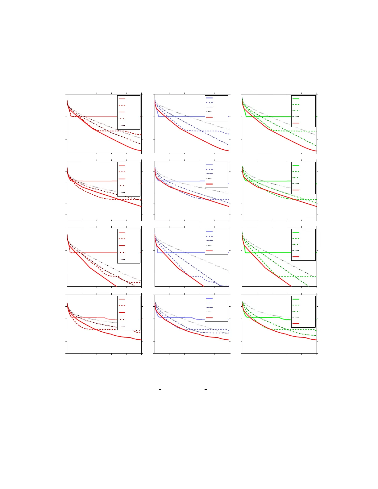
Con v ergence Rates of Inexact Pro ximal-Gradien t Metho ds for Con v ex Optimization Mark Sc hmidt mark.schmidt@inria.fr Nicolas Le Roux nicolas@le-roux.name F rancis Bac h francis.bach@ens.fr INRIA - SIERRA Pro ject - T eam Lab oratoire d’Informatique de l’ ´ Ecole Normale Sup ´ erieure P aris, F rance No vem b er 27, 2024 Abstract W e consider the problem of optimizing the sum of a smo oth conv ex function and a non-smo oth con vex function using p roximal-gradien t methods, where an error is presen t in the calculation of the gradien t of the smooth term or in the proximit y operator with resp ect to the non-smo oth term. W e show that b oth the basic pro ximal-gradien t method and the accelerated proximal-gradien t metho d achiev e the same conv ergence rate as in the error-free case, provided that the errors decrease at appropriate rates. Using these rates, we p erform as well as or b etter than a carefully chosen fixed error level on a set of structured sparsity problems. 1 In tro duction In recen t years the imp ortance of taking adv antage of the structure of con vex optimization problems has b ecome a topic of in tense researc h in the machine learning communit y . This is particularly true of tec hniques for non-smo oth optimization, where taking adv an tage of the structure of non-smo oth terms seems to b e crucial to obtaining go od p erformance. Pro ximal-gradient metho ds and ac c eler ate d pro ximal-gradient metho ds [1, 2] are among the most imp ortan t methods for taking adv antage of the structure of man y of the non- smo oth optimization problems that arise in practice. In particular, these methods address comp osite optimization problems of the form minimize x ∈ R d f ( x ) : = g ( x ) + h ( x ) , (1) where g and h are conv ex functions but only g is smo oth. One of the most w ell-studied instances of this t yp e of problem is ` 1 -regularized least squares [3, 4], minimize x ∈ R d 1 2 k Ax − b k 2 + λ k x k 1 , 1 where we use k · k to denote the standard ` 2 -norm. Pro ximal-gradient metho ds are an app ealing approac h for solving these t yp es of non-smo oth optimization problems b ecause of their fast theoretical con vergence rates and strong prac- tical p erformance. While classical subgradien t metho ds only achiev e an error level on the ob jective function of O (1 / √ k ) after k iterations, pro ximal-gradient metho ds hav e an error of O (1 /k ) while ac c eler ate d proximal-gradien t metho ds futher reduce this to O (1 /k 2 ) [1, 2]. That is, accelerated proximal-gradien t methods for non-smo oth conv ex optimization ac hieve the same optimal conv ergence rate that accelerated gradient metho ds ac hieve for smo oth optimization. Eac h iteration of a proximal-gradien t metho d requires the calculation of the proximit y op erator, pro x L ( y ) = arg min x ∈ R d L 2 k x − y k 2 + h ( x ) , (2) where L is the Lipschitz constan t of the gradien t of g . W e can efficien tly compute an analytic solution to this problem for sev eral notable choices of h , including the case of ` 1 -regularization and disjoin t group ` 1 -regularization [5, 6]. Ho wev er, in many scenarios the pro ximity operator ma y not ha ve an analytic solution, or it ma y b e very exp ensive to compute this solution exactly . This includes imp ortan t problems suc h as total-v ariation regularization and its generalizations like the graph-guided fused-LASSO [7, 8], nuclear- norm regularization and other regularizers on the singular v alues of matrices [9, 10], and differen t form ulations of ov erlapping group ` 1 -regularization with general groups [11, 12]. Despite the difficulty in computing the exact pro ximity op erator for these regularizers, efficien t metho ds hav e b een developed to compute appr oximate proximit y op erators in all of these cases ; accelerated pro jected gradien t and Newton-lik e methods that w ork with a smo oth dual problem hav e b een used to compute approximate pro ximity op erators in the context of total-v ariation regularization [7, 13], Krylov subspace metho ds and low-rank represen tations hav e b een used to compute approximate pro ximity op erators in the context of n uclear-norm regularization [9, 10], and v ariants of Dykstra’s algorithm (and related dual metho ds) hav e b een used to compute approximate proximit y op erators in the context of o verlapping group ` 1 -regularization [12, 14, 15]. It is known that pro ximal-gradient metho ds that use an approximate proximit y op erator con verge under only w eak assumptions [16, 17]; w e briefly review this and other related w ork in the next section. How ev er, despite the man y recent w orks sho wing impressive em- pirical p erformance of (accelerated) pro ximal-gradient metho ds that use an approximate pro ximity op erator [7, 9, 10, 13, 14, 15], up un til recently there w as no theoretical analysis on how the error in the calculation of the proximit y op erator affects the con vergence r ate of pro ximal-gradient metho ds. In this w ork, w e sho w in several contexts that, pro vided the error in the proximit y op erator calculation is controlled in an appropriate w a y , inexact pro ximal-gradient strategies achiev e the same conv ergence rates as the corresp onding exact metho ds. In particular, in Section 4 we first consider con vex ob jectives and analyze the in- exact proximal-gradien t (Prop osition 1) and accelerated pro ximal-gradient (Prop osition 2) metho ds. W e then analyze these tw o algorithms for strongly conv ex ob jectives (Prop osi- tion 3 and Prop osition 4). Note that, in these analyses, we also consider the p ossibility 2 that there is an error in the calculation of the gradient of g . W e then presen t an exp eri- men tal comparison of v arious inexact proximal-gradien t strategies in the con text of solving a structured sparsity problem (Section 5). 2 Related W ork The algorithm we shall fo cus on in this pap er is the proximal-gradien t metho d x k = pro x L  y k − 1 − (1 /L )( g 0 ( y k − 1 ) + e k )  , (3) where e k is the error in the calculation of the gradien t and the proximit y problem (2) is solv ed inexactly so that x k has an error of ε k in terms of the pro ximal ob jective function (2). In the basic proximal-gradien t method w e c ho ose y k = x k , while in the accelerated pro ximal- gradien t me thod we c ho ose y k = x k + β k ( x k − x k − 1 ) , where the sequence { β k } is chosen to accelerate the con vergence rate. There is a substan tial amoun t of work on metho ds that use an exact pro ximity operator but ha ve an error in the gradient calculation, corresp onding to the sp ecial case where ε k = 0 but e k is non-zero. F or e xample, when the e k are indep enden t, zero-mean, and finite- v ariance random v ariables, then pro ximal-gradient metho ds ac hieve the (optimal) error lev el of O (1 / √ k ) [18, 19]. This is different than the scenario w e analyze in this pap er since w e do not assume un biased nor indep enden t errors but instead consider a sequence of errors con verging to 0. This leads to faster conv ergence rates and makes our analysis applicable to the case of deterministic and ev en adversarial errors. Sev eral authors hav e recen tly analyzed the case of a fixed deterministic error in the gradien t, and shown that accelerated gradient metho ds achiev e the optimal con vergence rate up to some accuracy that depends on the fixed error lev el [20, 21, 22], while the earlier work of [23] analyzes the gradien t metho d in the con text of a fixed error lev el. This contrasts with our analysis where b y allo wing the error to c hange at ev ery iteration w e can ac hieve con vergence to the optimal solution. Also, w e can tolerate a large error in early iterations when we are far from the solution, whic h may lead to substan tial computational gains. Other authors ha ve analyzed the conv ergence rate of the gradient and pro jected-gradient metho ds with a decreasing sequence of errors [24, 25] but this analysis do es not consider the imp ortan t class of accelerated gradien t metho ds. In con trast, the analysis of [22] allows a decreasing sequence of errors (though conv ergence rates in this context are not explicitly mentioned) and considers the accelerated pro jected-gradien t metho d. Ho w ever, the authors of this w ork only consider the case of an exact pro jection step and they assume the av ailability of an oracle that yields global low er and upp er b ounds on the function. This non-intuitiv e oracle leads to a no vel analysis of smo othing metho ds, but also to slow er conv ergence rates than pro ximal-gradient metho ds. The analysis of [21] considers errors in b oth the gradien t and pro jection op erators for accelerated pro jected-gradien t metho ds but requires that the domain of the function is compact. None of these works consider proximal-gradien t metho ds. 3 In the con text of pr oximal-p oint algorithms, there is a substan tial literature on using inexact pro ximity op erators with a decreasing sequence of errors, dating back to the seminal work of Ro c k afellar [26]. Accelerated pro ximal-p oin t metho ds with a decreasing sequence of errors ha ve also b een examined, b eginning with [27]. How ev er, unlik e proximal-gradien t metho ds where the pro ximity op erator is only c omputed with resp ect to the non-smo oth function h , pro ximal-p oin t metho ds require the calculation of the proximit y op erator with resp ect to the full ob jective function. In the con text of comp osite optimization problems of the form (1), this requires the calculation of the proximit y op erator with resp ect to g + h . Since it ignores the structure of the problem, this proximit y op erator may b e as difficult to compute (even approximately) as the minimizer of the original problem. Con vergence of inexact proximal-gradien t metho ds can b e established with only weak as- sumptions on the metho d used to approximately solv e (2). F or example, we can establish that inexact pro ximal-gradient metho ds conv erge under some closedness assumptions on the mapping induced b y the approximate proximit y op erator, and the assumption that the algorithm used to compute the inexact proximit y op erator ac hieves sufficient descen t on problem (2) compared to the previous iteration x k − 1 [16]. Conv ergence of inexact pro ximal- gradien t metho ds can also b e established under the assumption that the norms of the errors are summable [17]. Ho w ever, these prior w orks did not consider the r ate of con vergence of inexact proximal-gradien t metho ds, nor did they consider accelerated proximal-gradien t metho ds. Indeed, the authors of [7] c hose to use the non-accelerated v ariant of the proximal- gradien t algorithm since even con v ergence of the accelerated proximal-gradien t metho d had not b een established under an inexact proximit y op erator. While preparing the final version of this work, [28] indep enden tly gav e an analysis of the accelerated proximal-gradien t metho d with an inexact proximit y op erator and a decreasing sequence of errors (assuming an exact gradient). F urther, their analysis leads to a w eaker dep endence on the errors than in our Prop osition 2. Ho wev er, while we only assume that the proximal problem can b e solved up to a certain accuracy , they make the m uch stronger assumption that the inexact proximit y op erator yields an ε k -sub differen tial of h [28, Defini- tion 2.1]. Our analysis can b e mo dified to give an impro ved dependence on the errors under this stronger assumption. In particular, the terms in √ ε i disapp ear from the expressions of A k , e A k and b A k . In the case of Prop ositions 1 and 2, this leads to the optimal con v ergence rate with a slo w er decay of ε i . More details ma y b e found after Lemma 2 in the Ap- p endix. More recently , [29] gav e an alternative analysis of an accelerated proximal-gradien t metho d with an inexact proximit y op erator and a decreasing sequence of errors (assuming an exact gradient), but under a non-intuitiv e assumption on the relationship b et ween the appro ximate s olution of the proximal problem and the ε k -sub differen tial of h . 3 Notation and Assumptions In this w ork, we assume that the smo oth function g in (1) is conv ex and differen tiable, and that its gradient g 0 is Lipschitz-con tinuous with constant L , meaning that for all x and y in R d w e ha v e k g 0 ( x ) − g 0 ( y ) k 6 L k x − y k . 4 This is a standard assumption in differen tiable optimization, see [30, § 2.1.1]. If g is twice- differen tiable, this corresp onds to the assumption that the eigenv alues of its Hessian are b ounded ab o ve by L . In Prop ositions 3 and 4 only , we will also assume that g is µ -strongly con vex (see [30, § 2.1.3]), meaning that for all x and y in R d w e ha v e g ( y ) > g ( x ) + h g 0 ( x ) , y − x i + µ 2 || y − x || 2 . Ho wev er, apart from Prop ositions 3 and 4, w e only assume that this holds with µ = 0, whic h is equiv alent to con vexit y of g . In con trast to these assumptions on g , we will only assume that h in (1) is a low er semi- con tinuous prop er conv ex function (see [31, § 1.2]), but will not assume that h is differentiable or Lipsc hitz-contin uous. This allo ws h to be an y real-v alued con v ex function, but also allo ws for the p ossibilit y that h is an extended real-v alued conv ex function. F or example, h could b e the indicator function of a con vex set, and in this case the pro ximity op erator b ecomes the pro jection op erator. W e will use x k to denote the parameter v ector at iteration k , and x ∗ to denote a minimizer of f . W e assume that suc h an x ∗ exists, but do not assume that it is unique. W e use e k to denote the error in the calculation of the gradient at iteration k , and we use ε k to denote the error in the pro ximal ob jective function ac hieved by x k , meaning that L 2 k x k − y k 2 + h ( x k ) 6 ε k + min x ∈ R d  L 2 k x − y k 2 + h ( x )  , (4) where y = y k − 1 − (1 /L )( g 0 ( y k − 1 ) + e k )). Note that the pro ximal optimization problem (2) is strongly conv ex and in practice we are often able to obtain such b ounds via a duality gap (e.g., see [12] for the case of o verlapping group ` 1 -regularization). 4 Con v ergence Rates of Inexact Pro ximal-Gradien t Metho ds In this section we presen t the analysis of the conv ergence rates of inexact proximal-gradien t metho ds as a function of the sequences of solution accuracies to the proximal problems { ε k } , and the sequences of magnitudes of the errors in the gradien t calculations {k e k k} . W e shall use ( H ) to denote the set of four assumptions which will b e made for eac h prop osition: • g is conv ex and has L -Lipsc hitz-contin uous gradient; • h is a lo wer semi-contin uous prop er conv ex function; • The function f = g + h attains its minim um at a certain x ∗ ∈ R n ; • x k is an ε k -optimal solution to the pro ximal problem (2) in the sense of (4). W e first consider the basic proximal-gradien t metho d in the con vex case : 5 Prop osition 1 (Basic pro ximal-gradien t metho d - Conv exity) Assume ( H ) and that we iter ate r e cursion (3) with y k = x k . Then, for al l k > 1 , we have f 1 k k X i =1 x i ! − f ( x ∗ ) 6 L 2 k  k x 0 − x ∗ k + 2 A k + p 2 B k  2 , (5) with A k = k X i =1 k e i k L + r 2 ε i L ! , B k = k X i =1 ε i L . The pro of may b e found in the Appendix. Note that while w e hav e stated the prop osition in terms of the function v alue achiev ed b y the a verage of the iterates, it trivially also holds for the iteration that ac hieves the low est function v alue. This result implies that the w ell- kno wn O (1 /k ) conv ergence rate for the gradien t metho d without errors stil l holds when b oth {k e k k} and { √ ε k } are summable. A sufficient condition to achiev e this is for k e k k and √ ε k to decrease as O (1 /k 1+ δ ) for any δ > 0. Note that a faster conv ergence of these tw o errors will not impro ve the con vergence rate but will yield a b etter constant factor. It is interesting to consider what happens if {k e k k} or { √ ε k } is not summable. F or instance, if k e k k and √ ε k decrease as O (1 /k ), then A k gro ws as O (log k ) (note that B k is alwa ys smaller than A k ) and the con vergence of the function v alues is in O  log 2 k k  . Finally , a necessary condition to obtain conv ergence is that the partial sums A k and B k need to b e in o ( √ k ). W e no w turn to the case of an ac c eler ate d proximal-gradien t metho d. W e fo cus on a basic v ariant of the algorithm where β k is set to ( k − 1) / ( k + 2) [32, Eq. (19) and (27)]: Prop osition 2 (Accelerated pro ximal-gradien t metho d - Conv exity) Assume ( H ) and that we iter ate r e cursion (3) with y k = x k + k − 1 k +2 ( x k − x k − 1 ) . Then, for al l k > 1 , we have f ( x k ) − f ( x ∗ ) 6 2 L ( k + 1) 2  k x 0 − x ∗ k + 2 e A k + q 2 e B k  2 , (6) with e A k = k X i =1 i k e i k L + r 2 ε i L ! , e B k = k X i =1 i 2 ε i L . In this case, w e require the series { k k e k k} and { k √ ε k } to b e summable to ac hieve the optimal O (1 /k 2 ) rate, whic h is an (unsurprisingly) stronger constraint than in the basic case. A sufficien t condition is for k e k k and √ ε k to decrease as O (1 /k 2+ δ ) for any δ > 0. Note that, as opp osed to Prop osition 1 that is stated for the av erage iterate, this b ound is for the last iterate x k . Again, it is in teresting to see what happ ens when the summabilit y assumption is not met. First, if k e k k or √ ε k decreases at a rate of O (1 /k 2 ), then k ( k e k k + √ e k ) decreases as O (1 /k ) and e A k gro ws as O (log k ) (note that e B k is alw ays smaller than e A k ), yielding a conv ergence rate of O  log 2 k k 2  for f ( x k ) − f ( x ∗ ). Also, and p erhaps more interestingly , if k e k k or √ ε k 6 decreases at a rate of O (1 /k ), Eq. (6) does not guaran tee con v ergence of the function v alues. More generally , the form of e A k and e B k indicates that errors hav e a greater effect on the accelerated metho d than on the basic metho d. Hence, as also discussed in [22], unlik e in the error-free case, the accelerated metho d ma y not necessarily b e b etter than the basic metho d b ecause it is more sensitiv e to errors in the computation. In the case where g is str ongly con vex it is p ossible to obtain linear con vergence rates that dep end on the ratio γ = µ/L, as opp osed to the sublinear conv ergence rates discussed ab ov e. In particular, w e obtain the follo wing conv ergence rate on the iterates of the basic proximal-gradien t metho d: Prop osition 3 (Basic pro ximal-gradien t metho d - Strong conv exit y) Assume ( H ), that g is µ -str ongly c onvex, and that we iter ate r e cursion (3) with y k = x k . Then, for al l k > 1 , we have: k x k − x ∗ k 6 (1 − γ ) k ( k x 0 − x ∗ k + ¯ A k ) , (7) with ¯ A k = k X i =1 (1 − γ ) − i k e i k L + r 2 ε i L ! . A consequence of this prop osition is that w e obtain a linear rate of conv ergence even in the presence of errors, pro vided that k e k k and √ ε k decrease linearly to 0. If they do so at a rate of Q 0 < (1 − γ ), then the conv ergence rate of k x k − x ∗ k is linear with constant (1 − γ ), as in the error-free algorithm. If we ha ve Q 0 > (1 − γ ), then the conv ergence of k x k − x ∗ k is linear with constant Q 0 . If w e hav e Q 0 = (1 − γ ), then k x k − x ∗ k conv erges to 0 as O ( k (1 − γ ) k ) = o  [(1 − γ ) + δ 0 ] k  for all δ 0 > 0. Finally , we consider the accelerated proximal-gradien t algorithm when g is strongly conv ex. W e fo cus on a basic v ariant of the algorithm where β k is set to (1 − √ γ ) / (1 + √ γ ) [30, § 2.2.1]: Prop osition 4 (Accelerated pro ximal-gradien t metho d - Strong conv exit y) Assume ( H ), that g is µ -str ongly c onvex, and that we iter ate r e cursion (3) with y k = x k + 1 − √ γ 1+ √ γ ( x k − x k − 1 ) . Then, for al l k > 1 , we have f ( x k ) − f ( x ∗ ) 6 (1 − √ γ ) k  p 2( f ( x 0 ) − f ( x ∗ )) + b A k r 2 µ + q b B k  2 , (8) with b A k = k X i =1  k e i k + p 2 Lε i  (1 − √ γ ) − i/ 2 , b B k = k X i =1 ε i (1 − √ γ ) − i . Note that while w e ha ve stated the result in terms of function v alues, w e obtain an analogous result on the iterates b ecause b y strong con vexit y of f w e hav e µ 2 || x k − x ∗ || 2 ≤ f ( x k ) − f ( x ∗ ) . 7 This proposition implies that w e obtain a linear rate of conv ergence in the presence of errors pro vided that || e k || 2 and ε k decrease linearly to 0. If they do so at a rate Q 0 < (1 − √ γ ), then the constan t is (1 − √ γ ), while if Q 0 > (1 − √ γ ) then the constan t will b e Q 0 . Thus, the accelerated inexact proximal-gradien t metho d will hav e a faster conv ergence rate than the exact basic proximal-gradien t metho d provided that Q 0 < (1 − γ ). Oddly , in our analysis of the strongly conv ex case, the accelerated metho d is less sensitive to errors than the basic metho d. Ho w ever, unlike the basic metho d, the accelerated metho d requires kno wing µ in addition to L . If µ is missp ecified, then the conv ergence rate of the accelerated metho d ma y be slo wer than the basic metho d. 5 Exp erimen ts W e tested the basic inexact proximal-gradien t and accelerated proximal-gradien t metho ds on the CUR-like factorization optimization problem in tro duced in [33] to appro ximate a giv en matrix W , min X 1 2 k W − W X W k 2 F + λ row n r X i =1 || X i || p + λ col n c X j =1 || X j || p . Under an appropriate choice of p , this optimization problem yields a matrix X with sparse ro ws and sparse columns, meaning that en tire rows and columns of the matrix X are set to exactly zero. In [33], the authors used an accelerated pro ximal-gradient metho d and chose p = ∞ since under this c hoice the proximit y op erator can b e computed exactly . How ev er, this has the undesirable effect that it also encourages all v alues in the same ro w (or column) to hav e the same magnitude. The more natural c hoice of p = 2 w as not explored since in this case there is no known algorithm to exactly compute the proximit y op erator. Our exp erimen ts fo cused on the case of p = 2. In this case, it is p ossible to very quickly compute an appro ximate pro ximity op erator using the block coordinate descent (BCD) algorithm presen ted in [12], which is equiv alent to the proximal v ariant of Dykstra’s algo- rithm introduced by [34]. In our implementation of the BCD metho d, we alternate b et ween computing the proximit y op erator with resp ect to the rows and to the columns. Since the BCD metho d allo ws us to compute a duality gap when solving the proximal problem, we can run the metho d until the dualit y gap is b elow a giv en error threshold ε k to find an x k +1 satisfying (4). In our exp erimen ts, w e used the four data sets examined by [33] 1 and we choose λ row = . 01 and λ col = . 01, which yielded approximately 25–40% non-zero en tries in X (depending on the data set). Rather than assuming w e are giv en the Lipsc hitz constan t L , on the first iteration we set L to 1 and following [2] w e double our estimate an ytime g ( x k ) > g ( y k − 1 ) + h g 0 ( y k − 1 ) , x k − y k − 1 i + ( L/ 2) || x k − y k − 1 || 2 . W e tested three different w ays to terminate the approximate pro ximal problem, eac h parameterized b y a parameter α : • ε k = 1 /k α : Running the BCD algorithm until the duality gap is b elo w 1 /k α . 1 The datasets are freely a v ailable at http://www.gems- system.org . 8 • ε k = α : Running the BCD algorithm until the duality gap is b elo w α . • n = α : Running the BCD algorithm for a fixed num b er of iterations α . Note that all three strategies lead to global conv ergence in the case of the basic proximal- gradien t method, the first t wo give a con vergence rate up to some fixed optimalit y tolerance, and in this pap er w e hav e shown that the first one (for large enough α ) yields a conv ergence rate for an arbitrary optimalit y tolerance. Note that the iterates pro duced by the BCD iterations are sp arse , so we exp ected the algorithms to sp end the ma jority of their time solving the proximit y problem. Th us, we used the function v alue against the num b er of BCD iterations as a measure of p erformance. W e plot the results after 500 BCD iterations for the four data sets for the pro ximal-gradient metho d in Figure 1, and the accelerated pro ximal-gradient metho d in Figure 2. In these plots, the first column v aries α using the c hoice ε k = 1 /k α , the second column v aries α using the c hoice ε k = α , and the third column v aries α using the c hoice n = α . W e also include one of the b est metho ds from the first column in the second and third columns as a reference. In the context of proximal-gradien t metho ds the choice of ε k = 1 /k 3 , whic h is one choice that ac hieves the fastest conv ergence rate according to our analysis, giv es the b est p erformance across all four data sets. How ev er, in these plots w e also see that reasonable p erformance can b e ac hieved b y an y of the three strategies ab o v e provided that α is c hosen carefully . F or example, c ho osing n = 3 or c ho osing ε k = 10 − 6 b oth give reasonable performance. How ever, these are only empirical observ ations for these data sets and they ma y b e ineffectiv e for other data sets or if we change the n umber of iterations, while we hav e given theoretical justification for the c hoice ε k = 1 /k 3 . Similar trends are observed for the case of accelerated pro ximal-gradien t metho ds, though the choice of ε k = 1 /k 3 (whic h no longer achiev es the fastest conv ergence rate according to our analysis) no longer dominates the other metho ds in the accelerated setting. F or the SRBCT data set the choice ε k = 1 /k 4 , whic h is a c hoice that ac hieves the fastest con vergence rate up to a p oly-logarithmic factor, yields b etter p erformance than ε k = 1 /k 3 . In terestingly , the only choice that yields the fastest p ossible con vergence rate ( ε k = 1 /k 5 ) had reasonable p erformance but did not give the b est p erformance on any data set. This seems to reflect the trade-off b et ween p erforming inner BCD iterations to ac hieve a small dualit y gap and p erforming outer gradien t iterations to decrease the v alue of f . Also, the constan t terms which were not taken into accoun t in the analysis do play an imp ortan t role here, due to the relativ ely small n umber of outer iterations p erformed. 6 Discussion An alternative to inexact pro ximal metho ds for solving structured sparsity problems are smo othing metho ds [35] and alternating direction methods [36]. Ho wev er, a ma jor dis- adv antage of both these approac hes is that the iterates are not sparse, so they can not tak e adv antage of the sparsity of the problem when running the algorithm. In con trast, the metho d prop osed in this pap er has the app ealing prop ert y that it tends to generate 9 100 200 300 400 500 10 −10 10 −5 10 0 ε k = 1/k ε k = 1/k 2 ε k = 1/k 3 ε k = 1/k 4 ε k = 1/k 5 100 200 300 400 500 10 −10 10 −5 10 0 n=1 n=2 n=3 n=5 ε k = 1/k 3 100 200 300 400 500 10 −10 10 −5 10 0 ε k =1e−2 ε k =1e−4 ε k =1e−6 ε k =1e−10 ε k = 1/k 3 100 200 300 400 500 10 −10 10 −8 10 −6 10 −4 10 −2 10 0 ε k = 1/k ε k = 1/k 2 ε k = 1/k 3 ε k = 1/k 4 ε k = 1/k 5 100 200 300 400 500 10 −10 10 −8 10 −6 10 −4 10 −2 10 0 n=1 n=2 n=3 n=5 ε k = 1/k 3 100 200 300 400 500 10 −10 10 −8 10 −6 10 −4 10 −2 10 0 ε k =1e−2 ε k =1e−4 ε k =1e−6 ε k =1e−10 ε k = 1/k 3 100 200 300 400 500 10 −10 10 −5 10 0 ε k = 1/k ε k = 1/k 2 ε k = 1/k 3 ε k = 1/k 4 ε k = 1/k 5 100 200 300 400 500 10 −10 10 −5 10 0 n=1 n=2 n=3 n=5 ε k = 1/k 3 100 200 300 400 500 10 −10 10 −5 10 0 ε k =1e−2 ε k =1e−4 ε k =1e−6 ε k =1e−10 ε k = 1/k 3 100 200 300 400 500 10 −10 10 −8 10 −6 10 −4 10 −2 10 0 ε k = 1/k ε k = 1/k 2 ε k = 1/k 3 ε k = 1/k 4 ε k = 1/k 5 100 200 300 400 500 10 −10 10 −8 10 −6 10 −4 10 −2 10 0 n=1 n=2 n=3 n=5 ε k = 1/k 3 100 200 300 400 500 10 −10 10 −8 10 −6 10 −4 10 −2 10 0 ε k =1e−2 ε k =1e−4 ε k =1e−6 ε k =1e−10 ε k = 1/k 3 Figure 1: Ob jective function against num b er of proximal iterations for the proximal-gradien t metho d with different strategies for terminating the approximate proximit y calculation. F rom top to b ottom w e hav e the 9 T umors , Br ain T umor1 , L eukemia1 , and SRBCT data sets. 10 100 200 300 400 500 10 −10 10 −5 10 0 ε k = 1/k ε k = 1/k 2 ε k = 1/k 3 ε k = 1/k 4 ε k = 1/k 5 100 200 300 400 500 10 −10 10 −5 10 0 n=1 n=2 n=3 n=5 ε k = 1/k 4 100 200 300 400 500 10 −10 10 −5 10 0 ε k =1e−2 ε k =1e−4 ε k =1e−6 ε k =1e−10 ε k = 1/k 4 100 200 300 400 500 10 −10 10 −8 10 −6 10 −4 10 −2 10 0 ε k = 1/k ε k = 1/k 2 ε k = 1/k 3 ε k = 1/k 4 ε k = 1/k 5 100 200 300 400 500 10 −10 10 −8 10 −6 10 −4 10 −2 10 0 n=1 n=2 n=3 n=5 ε k = 1/k 4 100 200 300 400 500 10 −10 10 −8 10 −6 10 −4 10 −2 10 0 ε k =1e−2 ε k =1e−4 ε k =1e−6 ε k =1e−10 ε k = 1/k 4 100 200 300 400 500 10 −10 10 −5 10 0 ε k = 1/k ε k = 1/k 2 ε k = 1/k 3 ε k = 1/k 4 ε k = 1/k 5 100 200 300 400 500 10 −10 10 −5 10 0 n=1 n=2 n=3 n=5 ε k = 1/k 4 100 200 300 400 500 10 −10 10 −5 10 0 ε k =1e−2 ε k =1e−4 ε k =1e−6 ε k =1e−10 ε k = 1/k 4 100 200 300 400 500 10 −10 10 −8 10 −6 10 −4 10 −2 10 0 ε k = 1/k ε k = 1/k 2 ε k = 1/k 3 ε k = 1/k 4 ε k = 1/k 5 100 200 300 400 500 10 −10 10 −8 10 −6 10 −4 10 −2 10 0 n=1 n=2 n=3 n=5 ε k = 1/k 4 100 200 300 400 500 10 −10 10 −8 10 −6 10 −4 10 −2 10 0 ε k =1e−2 ε k =1e−4 ε k =1e−6 ε k =1e−10 ε k = 1/k 4 Figure 2: Ob jective function against num b er of proximal iterations for the ac c eler ate d pro ximal-gradient metho d with different strategies for terminating the approximate prox- imit y calculation. F rom top to b ottom w e hav e the 9 T umors , Br ain T umor1 , L eukemia1 , and SRBCT data sets. 11 sparse iterates. F urther, the accelerated smo othing metho d only has a conv ergence rate of O (1 /k ), and the p erformance of alternating direction methods is often sensitive to the exact c hoice of their p enalt y parameter. On the other hand, while our analysis suggests using a sequence of errors like O (1 /k α ) for α large enough, the practical performance of inexact pro ximal-gradients metho ds will b e sensitive to the exac t choice of this sequence. Although w e hav e illustrated the use of our results in the context of a structured sparsit y problem, inexact pro ximal-gradien t metho ds are also used in other applications such as total-v ariation [7, 8] and n uclear-norm [9, 10] regularization. This work pro vides a theoreti- cal justification for using inexact proximal-gradien t metho ds in these and other applications, and suggests some guidelines for practioners that do not wan t to lose the app ealing conv er- gence rates of these methods. F urther, although our experiments and m uch of our discussion fo cus on errors in the calculation of the proximit y operator, our analysis also allo ws for an error in the calculation of the gradien t. This may also be useful in a v ariety of con texts. F or example, errors in the calculation of the gradient arise when fitting undirected graphical mo dels and using an iterativ e metho d to appro ximate the gradient of the log-partition func- tion [37]. Other examples include using a reduced set of training examples within kernel metho ds [38] or subsampling to solv e semidefinite programming problems [39]. In our analysis, we assume that the smo othness constan t L is kno wn, but it would b e in teresting to extend metho ds for estimating L in the exact case [2] to the case of inexact algorithms. In the context of accelerated metho ds for strongly conv ex optimization, our analysis also assumes that µ is known, and it w ould b e interesting to explore v ariants that do not make this assumption. W e also note that if the basic pro ximal-gradient metho d is giv en kno wledge of µ , then our analysis can b e modified to obtain a faster linear conv ergence rate of (1 − γ ) / (1 + γ ) instead of (1 − γ ) for strongly-conv ex optimization using a step size of 2 / ( µ + L ), see Theorem 2.1.15 of [30]. Finally , we note that there has b een recen t in terest in inexact proximal Newton-like metho ds [40], and it w ould b e interesting to analyze the effect of errors on the conv ergence rates of these metho ds. Ac kno wledgements Mark Sc hmidt, Nicolas Le Roux, and F rancis Bac h are supp orted b y the Europ ean Researc h Council (SIERRA-ERC-239993). App endix: Pro ofs of the prop ositions W e first pro ve a lemma whic h will b e used for the propositions. Lemma 1 Assume that the nonne gative se quenc e { u k } satisfies the fol lowing r e cursion for al l k > 1 : u 2 k 6 S k + k X i =1 λ i u i , 12 with { S k } an incr e asing se quenc e, S 0 > u 2 0 and λ i > 0 for al l i . Then, for al l k > 1 , then u k 6 1 2 k X i =1 λ i +   S k + 1 2 k X i =1 λ i ! 2   1 / 2 Pro of W e prov e the result by induction. It is true for k = 0 (by assumption). W e assume it is true for k − 1, and we denote b y v k − 1 = max { u 1 , . . . , u k − 1 } . F rom the recursion, we th us get ( u k − λ k / 2) 2 6 S k + λ 2 k 4 + v k − 1 k − 1 X i =1 λ i leading to u k 6 λ k 2 + S k + λ 2 k 4 + v k − 1 k − 1 X i =1 λ i ! 1 / 2 and thus v k 6 max    v k − 1 , λ k 2 + S k + λ 2 k 4 + v k − 1 k − 1 X i =1 λ i ! 1 / 2    The t wo terms in the maxim um are equal if v 2 k − 1 = S k + v k − 1 P k i =1 λ i , i.e., for v ∗ k − 1 = 1 2 P k i =1 λ i +  S k +  1 2 P k i =1 λ i  2  1 / 2 . If v k − 1 6 v ∗ k − 1 , then v k 6 v ∗ k − 1 since the tw o terms in the max are increasing functions of v k − 1 . If v k − 1 > v ∗ k − 1 , then v k − 1 > λ k 2 +  S k + λ 2 k 4 + v k − 1 P k − 1 i =1 λ i  1 / 2 . Hence, v k 6 v k − 1 , and the induction hypotheses ensure that the prop ert y is satisfied for k . The follo wing lemma will allow us to characterize the elements of the ε k -sub differen tial of h at x k , ∂ ε k h ( x k ). As a reminder, the ε -sub differential of a con vex function a at x is the set of vectors y such that a ( t ) − a ( x ) > y > ( t − x ) − ε for all t . Lemma 2 If x i is an ε i -optimal solution to the pr oximal pr oblem (2) in the sense of (4) , then ther e exists f i such that k f i k 6 q 2 ε i L and L  y i − 1 − x i − 1 L ( g 0 ( y i − 1 ) + e i ) − f i  ∈ ∂ ε i h ( x i ) . Pro of W e first recall some prop erties of ε -sub differen tials (see, e.g., [41, Section 4.3] for more details). By definition, x is an ε -minimizer of a conv ex function a if and only if a ( x ) 6 inf y ∈ R n a ( y ) + ε . This is equiv alent to 0 b elonging to the ε -sub differen tial ∂ ε a ( x ). If a = a 1 + a 2 , where b oth a 1 and a 2 are conv ex, w e hav e ∂ ε a ( x ) ⊂ ∂ ε a 1 ( x ) + ∂ ε a 2 ( x ). 13 If a 1 ( x ) = L 2 k x − z k 2 , then ∂ ε a 1 ( x ) =  y ∈ R n     L 2    x − z − y L    2 6 ε  =  y ∈ R n , y = Lx − Lz + Lf     L 2 k f k 2 6 ε  . If a 2 = h and x is an ε -minimizer of a 1 + a 2 , then 0 b elongs to ∂ ε a ( x ). Since ∂ ε a ( x ) ⊂ ∂ ε a 1 ( x ) + ∂ ε a 2 ( x ), w e hav e that 0 is the sum of an elemen t of ∂ ε a 1 ( x ) and of an element of ∂ ε h ( x ). Hence, there is an f such that Lz − Lx − Lf ∈ ∂ ε h ( x ) with k f k 6 r 2 ε L . (9) Using z = y i − 1 − (1 /L )( g 0 ( y i − 1 ) + e i ) and x = x i , this implies that there exists f i suc h that k f i k 6 q 2 ε i L and L  y i − 1 − x i − 1 L ( g 0 ( y i − 1 ) + e i ) − f i  ∈ ∂ ε i h ( x i ) . In [28, Definition 2.1], Eq. (9) is replaced by Lz − Lx ∈ ∂ ε h ( x ). Hence, their definition of an appro ximate solution is equiv alen t to ours but using f = 0. If w e replace k f i k b y 0 in the pro of of Prop osition 2, w e get the O (1 /k 2 ) con vergence rate using any sequence of errors { ε k } necessary to achiev e the O (1 /k 2 ) rate in [28, Th. 4.4]. W e can also make the same assumption on f in Proposition 1 to ac hieve the optimal con v ergence rate with a decay of √ ε k in O  1 /k 0 . 5+ δ  instead of O  1 /k 1+ δ  . 6.1 Basic pro ximal-gradien t metho d with errors in the con vex case W e now giv e the pro of of Prop osition of 1. Pro of Since x k is an ε k -optimal solution to the proximal problem (2) in the sense of (4), w e can use Lemma 2 to yield that there exists f k suc h that k f k k 6 q 2 ε k L and L  x k − 1 − x k − 1 L ( g 0 ( x k − 1 ) + e k ) − f k  ∈ ∂ ε i h ( x k ) . W e now b ound g ( x i ) and h ( x i ) as follows: g ( x i ) 6 g ( x i − 1 ) +  g 0 ( x i − 1 ) , x i − x i − 1  + L 2 k x i − x i − 1 k 2 using L-Lipschitz gradient and the conv exity of g , 6 g ( x ∗ ) +  g 0 ( x i − 1 ) , x i − 1 − x ∗  +  g 0 ( x i − 1 ) , x i − x i − 1  + L 2 k x i − x i − 1 k 2 using conv exity of g . 14 Using the ε i -subgradien t, we ha ve h ( x i ) 6 h ( x ∗ ) −  g 0 ( x i − 1 ) + e i + L ( x i + f i − x i − 1 ) , x i − x ∗  + ε i . Adding the tw o together, w e get: f ( x i ) = g ( x i ) + h ( x i ) = f ( x ∗ ) + L 2 k x i − x i − 1 k 2 − L h x i − x i − 1 , x i − x ∗ i + ε i − h e i + Lf i , x i − x ∗ i = f ( x ∗ ) + L 2 h x i − x i − 1 , x i − x i − 1 − 2 x i + 2 x ∗ i + ε i − h e i + Lf i , x i − x ∗ i = f ( x ∗ ) + L 2 h x i − x ∗ − ( x i − 1 − x ∗ ) , ( x ∗ − x i ) + ( x ∗ − x i − 1 ) i + ε i − h e i + Lf i , x i − x ∗ i = f ( x ∗ ) − L 2 k x i − x ∗ k 2 + L 2 k x i − 1 − x ∗ k 2 + ε i − h e i + Lf i , x i − x ∗ i f ( x i ) 6 f ( x ∗ ) − L 2 k x i − x ∗ k 2 + L 2 k x i − 1 − x ∗ k 2 + ε i + ( k e i k + p 2 Lε i ) · k x i − x ∗ k using Cauch y-Sch wartz and k f i k 6 q 2 ε i L . Mo ving f ( x ∗ ) on the other side and summing from i = 1 to k , we get: k X i =1 [ f ( x i ) − f ( x ∗ )] 6 − L 2 k x k − x ∗ k 2 + L 2 k x 0 − x ∗ k 2 + k X i =1 ε i + k X i =1 h ( k e i k + p 2 Lε i ) · k x i − x ∗ k i , i.e. k X i =1 [ f ( x i ) − f ( x ∗ )] + L 2 k x k − x ∗ k 2 6 L 2 k x 0 − x ∗ k 2 + k X i =1 ε i + k X i =1 h ( k e i k + p 2 Lε i ) · k x i − x ∗ k i . (10) Eq. (10) has tw o purp oses. The first one is to b ound the v alues of k x i − x ∗ k using the recursiv e definition. Once w e hav e a b ound on these quantities, we shall b e able to b ound the function v alues using only k x 0 − x ∗ k and the v alues of the errors. 6.1.1 Bounding k x i − x ∗ k W e now need to b ound the quantities k x i − x ∗ k in terms of k x 0 − x ∗ k , e i and ε i . Dropping the first term in Eq. (10), whic h is positive due to the optimalit y of f ( x ∗ ), we hav e: k x k − x ∗ k 2 6 k x 0 − x ∗ k 2 + 2 L k X i =1 ε i + 2 k X i =1 " k e i k L + r 2 ε i L ! · k x i − x ∗ k # W e now use Lemma 1 (using S k = k x 0 − x ∗ k 2 + 2 L P k i =1 ε i and λ i = 2  k e i k L + q 2 ε i L  ) to get k x k − x ∗ k 6 k X i =1 k e i k L + r 2 ε i L ! +   k x 0 − x ∗ k 2 + 2 L k X i =1 ε i + " k X i =1 k e i k L + r 2 ε i L !# 2   1 / 2 . 15 Denoting A k = P k i =1  k e i k L + q 2 ε i L  and B k = P k i =1 ε i L , we get k x k − x ∗ k 6 A k +  k x 0 − x ∗ k 2 + 2 B k + A 2 k  1 / 2 . Since A i and B i are increasing sequences ( k e i k and ε i b eing p ositiv e), we hav e for i 6 k k x i − x ∗ k 6 A i +  k x 0 − x ∗ k 2 + 2 B i + A 2 i  1 / 2 6 A k +  k x 0 − x ∗ k 2 + 2 B k + A 2 k  1 / 2 6 A k + k x 0 − x ∗ k + p 2 B k + A k using the p ositivity of k x 0 − x ∗ k 2 , B k and A 2 k . 6.1.2 Bounding the function v alues No w that w e hav e a common b ound for all k x i − x ∗ k with i 6 k , w e can upp er-bound the righ t-hand side of Eq. (10) using only terms dep ending on k x 0 − x ∗ k , e i and ε i . Indeed, discarding L 2 k x k − x ∗ k 2 whic h is p ositiv e, Eq. (10) b ecomes k X i =1 [ f ( x i ) − f ( x ∗ )] 6 L 2 k x 0 − x ∗ k 2 + LB k + LA k ( A k + k x 0 − x ∗ k + p 2 B k + A k ) 6 L 2 k x 0 − x ∗ k 2 + LB k + 2 LA 2 k + LA k k x 0 − x ∗ k + LA k p 2 B k 6 L 2  k x 0 − x ∗ k + 2 A k + p 2 B k  2 . Since f is con vex, we get f 1 k k X i =1 x i ! − f ( x ∗ ) 6 1 k k X i =1 [ f ( x i ) − f ( x ∗ )] 6 L 2 k  k x 0 − x ∗ k + 2 A k + p 2 B k  2 . 6.2 Accelerated pro ximal-gradient metho d with errors in the con v ex case W e now giv e the pro of of Prop osition 2. Pro of Defining θ k = 2 / ( k + 1) v k = x k − 1 + 1 θ k ( x k − x k − 1 ) , 16 w e can rewrite the up date for y k as y k = (1 − θ k +1 ) x k + θ k +1 v k , b ecause (1 − θ k +1 ) x k + θ k +1 v k = (1 − 2 k + 2 ) x k + 2 k + 2 [ x k − 1 + k + 1 2 ( x k − x k − 1 )] = x k − 2 k + 2 ( x k − x k − 1 ) + k + 1 k + 2 ( x k − x k − 1 ) = x k − k − 1 k + 2 ( x k − x k − 1 ) = y k . Because g 0 is Lipschitz and g is conv ex, we get for any z that g ( x k ) 6 g ( y k − 1 ) +  g 0 ( y k − 1 ) , x k − y k − 1  + L 2 k x k − y k − 1 k 2 6 g ( z ) +  g 0 ( y k − 1 ) , y k − 1 − z  +  g 0 ( y k − 1 ) , x k − y k − 1  + L 2 k x k − y k − 1 k 2 . Because − [ g 0 ( y k − 1 ) + e k + L ( x k + f k − y k − 1 )] ∈ ∂ ε k h ( x k ), we hav e for an y z that h ( x k ) 6 ε k + h ( z ) +  L ( y k − 1 − x k ) − g 0 ( y k − 1 ) − e k + Lf k , x k − z  = ε k + h ( z ) +  g 0 ( y k − 1 ) , z − x k  + L h x k − y k − 1 , z − x k i + h e k + Lf k , z − x k i Adding these b ounds together giv es: g ( x k ) + h ( x k ) = f ( x k ) 6 ε k + f ( z ) + L h x k − y k − 1 , z − x k i + L 2 k x k − y k − 1 k 2 + h e k + Lf k , z − x k i Cho osing z = θ k x ∗ + (1 − θ k ) x k − 1 giv es f ( x k ) 6 ε k + f ( θ k x ∗ + (1 − θ ) x k − 1 ) + L h x k − y k − 1 , θ k x ∗ + (1 − θ k ) x k − 1 − x k i + L 2 k x k − y k − 1 k 2 + h e k + Lf k , θ k x ∗ + (1 − θ k ) x k − 1 − x k i 6 ε k + θ k f ( x ∗ ) + (1 − θ k ) f ( x k − 1 ) + L h x k − y k − 1 , θ k x ∗ + (1 − θ k ) x k − 1 − x k i + L 2 k x k − y k − 1 k 2 + h e k + Lf k , θ k x ∗ + (1 − θ k ) x k − 1 − x k i (11) using the conv exit y of f and the fact that θ k is in [0 , 1]. Since θ k x ∗ + (1 − θ k ) x k − 1 − x k = θ k ( x ∗ − v k ) and x k − y k − 1 = θ k v k + (1 − θ k ) x k − 1 − y k − 1 = θ k v k − θ k v k − 1 , 17 w e ha v e L h x k − y k − 1 , θ k x ∗ + (1 − θ k ) x k − 1 − x k i = Lθ 2 k h v k − v k − 1 , x ∗ − v k i = − Lθ 2 k k v k − x ∗ k 2 + Lθ 2 k h v k − x ∗ , v k − 1 − x ∗ i (12) L 2 k x k − y k − 1 k 2 = Lθ 2 k 2 k v k − v k − 1 k 2 = Lθ 2 k 2  k v k − x ∗ k 2 + k v k − 1 − x ∗ k 2 − 2 h v k − x ∗ , v k − 1 − x ∗ i  (13) h e k + Lf k , θ k x ∗ + (1 − θ k ) x k − 1 − x k i = θ k h e k + Lf k , x ∗ − v k i . Summing Eq. (12) and (13), we get L h x k − y k − 1 , θ k x ∗ + (1 − θ k ) x k − 1 − x k i + L 2 k x k − y k − 1 k 2 = Lθ 2 k 2  k v k − 1 − x ∗ k 2 − k v k − x ∗ k 2  Mo ving all function v alues in Eq. (11) to the left-side, we then get f ( x k ) − θ k f ( x ∗ ) − (1 − θ k ) f ( x k − 1 ) 6 Lθ 2 k  k v k − 1 − x ∗ k 2 − k v k − x ∗ k 2  + ε k + θ k h e k + Lf k , x ∗ − v k i . Reordering the terms and dividing by θ 2 k giv es 1 θ 2 k ( f ( x k ) − f ( x ∗ ))+ L 2 k v k − x ∗ k 2 6 1 − θ k θ 2 k ( f ( x k − 1 ) − f ( x ∗ ))+ L 2 k v k − 1 − x ∗ k 2 + ε k θ 2 k + 1 θ k h e k + Lf k , x ∗ − v k i . No w w e use that for all k greater than or equal to 1, 1 − θ k θ 2 k 6 1 θ 2 k − 1 to apply this recursiv ely and obtain 1 θ 2 k ( f ( x k ) − f ( x ∗ )) + L 2 k v k − x ∗ k 2 6 1 − θ 0 θ 2 0 ( f ( x 0 ) − f ( x ∗ )) + L 2 k v 0 − x ∗ k 2 + k X i =1 ε i θ 2 i + k X i =1 1 θ i ( k e i k + p 2 Lε i ) · k x ∗ − v i k using k f i k 6 q 2 ε i L . Since v 0 = x 0 and θ 0 = 2, we get f ( x k ) − f ( x ∗ )+ Lθ 2 k 2 k v k − x ∗ k 2 6 Lθ 2 k 2 k x 0 − x ∗ k 2 + θ 2 k k X i =1 ε i θ 2 i + θ 2 k k X i =1 1 θ i  k e i k + p 2 Lε i  ·k x ∗ − v i k . (14) As in the previous pro of, we will no w use Eq. (14) to first b ound the v alues of k v i − x ∗ k then, using these b ounds, b ound the function v alues. 18 6.2.1 Bounding k v i − x ∗ k W e now need to b ound the quan tities k v i − x ∗ k in terms of k x 0 − x ∗ k , e i and ε i . k v k − x ∗ k 2 6 k x 0 − x ∗ k 2 + 2 L k X i =1 ε i θ 2 i + k X i =1 2 θ i k e i k L + r 2 ε i L ! · k x ∗ − v i k . Since θ i = 2 / ( i + 1), 1 θ i = i +1 2 6 i since i > 1. Thus, we ha ve k v k − x ∗ k 2 6 k x 0 − x ∗ k 2 + 2 L k X i =1 i 2 ε i + k X i =1 2 i k e i k L + r 2 ε i L ! · k x ∗ − v i k . F rom Lemma 1 (using S k = k x 0 − x ∗ k 2 + 2 L P k i =1 i 2 ε i and λ i = 2 i  k e i k L + q 2 ε i L  ), and denoting e A k = P k i =1 i  k e i k L + q 2 ε i L  and e B k = P k i =1 i 2 ε i L , we get k v k − x ∗ k 6 e A k +  k x 0 − x ∗ k 2 + 2 e B k + e A 2 k  1 / 2 . Since e A i and e B i are increasing sequences, w e also ha ve for i 6 k : k v i − x ∗ k 6 e A i +  k x 0 − x ∗ k 2 + 2 e B i + e A 2 i  1 / 2 6 k x 0 − x ∗ k + 2 e A i + e B 1 / 2 i √ 2 6 k x 0 − x ∗ k + 2 e A k + e B 1 / 2 k √ 2 . 6.2.2 Bounding the function v alues Dropping Lθ 2 k 2 k v k − x ∗ k 2 in Eq. (14) (since it is positive), w e th us hav e f ( x k ) − f ( x ∗ ) 6 Lθ 2 k 2  k x 0 − x ∗ k 2 + 2 e B k + 2 e A k  k x 0 − x ∗ k + 2 e A k + q 2 e B k  6 Lθ 2 k 2  k x 0 − x ∗ k 2 + 2 e B k + 2 e A k k x 0 − x ∗ k + 4 e A 2 k + 2 e A k q 2 e B k  6 Lθ 2 k 2  k x 0 − x ∗ k + 2 e A k + q 2 e B k  2 and 1 θ 2 k ( f ( x k ) − f ( x ∗ )) 6 L 2  k x 0 − x ∗ k + 2 e A k + q 2 e B k  2 . 19 6.3 Basic proximal-gradien t metho d with errors in the strongly con v ex case Belo w is the pro of of Prop osition 3 Pro of Again, there exists f i suc h that k f i k 6 q 2 ε i L and L  x i − 1 − x i − 1 L ( g 0 ( x i − 1 ) + e i ) − f i  ∈ ∂ ε i h ( x i ) . Since x ∗ is optimal, we ha ve that x ∗ = pro x L  x ∗ − 1 L g 0 ( x ∗ )  . W e first separate f k , the error in the proximal, from the rest: k x k − x ∗ k 2 =     pro x L  x k − 1 − 1 L g 0 ( x k − 1 ) − 1 L e k  + f k − prox L  x ∗ − 1 L g 0 ( x ∗ )      2 =     pro x L  x k − 1 − 1 L g 0 ( x k − 1 ) − 1 L e k  − prox L  x ∗ − 1 L g 0 ( x ∗ )      2 + k f k k 2 + 2  f k , pro x L  x k − 1 − 1 L g 0 ( x k − 1 ) − 1 L e k  − prox L  x ∗ − 1 L g 0 ( x ∗ )  6     pro x L  x k − 1 − 1 L g 0 ( x k − 1 ) − 1 L e k  − prox L  x ∗ − 1 L g 0 ( x ∗ )      2 + 2 ε k L + 2 r 2 ε k L     pro x L  x k − 1 − 1 L g 0 ( x k − 1 ) − 1 L e k  − prox L  x ∗ − 1 L g 0 ( x ∗ )      using Cauch y-Sch wartz and k f k k 6 q 2 ε k L 6     x k − 1 − 1 L g 0 ( x k − 1 ) − 1 L e k − x ∗ + 1 L g 0 ( x ∗ )     2 + 2 ε k L + 2 r 2 ε k L     x k − 1 − 1 L g 0 ( x k − 1 ) − 1 L e k − x ∗ + 1 L g 0 ( x ∗ )     using the non-expansiveness of the proximal 6     x k − 1 − 1 L g 0 ( x k − 1 ) − 1 L e k − x ∗ + 1 L g 0 ( x ∗ )     2 + 2 ε k L + 2 r 2 ε k L      x k − 1 − x ∗ − 1 L ( g 0 ( x k − 1 ) − g 0 ( x ∗ ))     + k e k k L  using the triangular inequalit y . 20 W e contin ue this computation, but no w separating e k , the error in the gradient, from the rest: k x k − x ∗ k 2 = k x k − 1 − x ∗ − 1 L ( g 0 ( x k − 1 ) − g 0 ( x ∗ )) k 2 + k e k k 2 L 2 − 2 L  e k , x k − 1 − x ∗ − 1 L ( g 0 ( x k − 1 ) − 1 L g 0 ( x ∗ ))  + 2 ε k L + 2 r 2 ε k L  k x k − 1 − x ∗ − 1 L ( g 0 ( x k − 1 ) − g 0 ( x ∗ )) k + k e k k L  6 k x k − 1 − x ∗ − 1 L ( g 0 ( x k − 1 ) − g 0 ( x ∗ )) k 2 + k e k k 2 L 2 + 2 L k e k kk x k − 1 − x ∗ − 1 L ( g 0 ( x k − 1 ) − g 0 ( x ∗ )) k + 2 ε k L + 2 r 2 ε k L  k x k − 1 − x ∗ − 1 L ( g 0 ( x k − 1 ) − g 0 ( x ∗ )) k + k e k k L  using Cauch y-Sch wartz 6 k x k − 1 − x ∗ − 1 L ( g 0 ( x k − 1 ) − g 0 ( x ∗ )) k 2 + k e k k 2 L 2 + 2 ε k L + 2 L r 2 ε k L k e k k + 2 k e k k L + 2 r 2 ε k L !     x k − 1 − x ∗ − 1 L ( g 0 ( x k − 1 ) − g 0 ( x ∗ ))     . W e now need to bound   x k − 1 − x ∗ − 1 L ( g 0 ( x k − 1 ) − g 0 ( x ∗ ))   to get the final result. W e ha ve: k x k − 1 − x ∗ − 1 L ( g 0 ( x k − 1 ) − g 0 ( x ∗ )) k 2 = k x k − 1 − x ∗ k 2 + 1 L 2 k g 0 ( x k − 1 ) − g 0 ( x ∗ ) k 2 − 2 L  g 0 ( x k − 1 ) − g 0 ( x ∗ ) , x k − 1 − x ∗  6 k x k − 1 − x ∗ k 2 + 1 L 2 k g 0 ( x k − 1 ) − g 0 ( x ∗ ) k 2 − 2 L  1 L + µ k g 0 ( x k − 1 ) − g 0 ( x ∗ ) k 2 + Lµ L + µ k x k − 1 − x ∗ k 2  using theorem 2.1.12 of [30] = (1 − 2 µ L + µ ) k x k − 1 − x ∗ k 2 + 1 L  1 L − 2 L + µ  k g 0 ( x k − 1 ) − g 0 ( x ∗ ) k 2 6 (1 − 2 µ L + µ ) k x k − 1 − x ∗ k 2 + µ 2 L ( 1 L − 2 L + µ ) k x k − 1 − x ∗ k 2 using the negativity of 1 L − 2 L + µ and the strong con vexit y of g =  1 − µ L  2 k x k − 1 − x ∗ k 2 . Th us k x k − x ∗ k 2 6  1 − µ L  2 k x k − 1 − x ∗ k 2 + k e k k 2 L 2 + 2 ε k L + 2 L r 2 ε k L k e k k + 2 k e k k L + 2 r 2 ε k L !  1 − µ L  k x k − 1 − x ∗ k = "  1 − µ L  k x k − 1 − x ∗ k + k e k k L + r 2 ε k L # 2 . 21 T aking the square ro ot of b oth sides and applying the b ound recursively yields k x k − x ∗ k 6  1 − µ L  k k x 0 − x ∗ k + k X i =1  1 − µ L  k − i k e i k L + r 2 ε i L ! . 6.4 Accelerated proximal-gradien t metho d with errors in the strongly con v ex case W e now giv e the pro of of Prop osition 4. Pro of W e hav e (following [30]) x k = y k − 1 − 1 L g 0 ( y k − 1 ) . W e define α 2 k = (1 − α k ) α 2 k − 1 + µ L α k v k = x k − 1 + 1 α k − 1 ( x k − x k − 1 ) θ k = α k − µ L 1 − µ L y k = x k + θ k ( v k − x k ) . If we choose α 0 = √ γ , then this yields y k = x k + 1 − √ γ 1 + √ γ ( x k − x k − 1 ) . W e can bound g ( x k ) with g ( x k ) 6 g ( y k − 1 ) + h g 0 ( y k − 1 ) , x k − y k − 1 i + L 2 k x k − y k − 1 k 2 using the conv exit y of g 6 g ( z ) + h g 0 ( y k − 1 ) , y k − 1 − z i + h g 0 ( y k − 1 ) , x k − y k − 1 i + L 2 k x k − y k − 1 k 2 − µ 2 k y k − 1 − z k 2 using the µ -strong con vexit y of g . Using Lemma 2, w e hav e that − [ g 0 ( y k − 1 ) + e k + L ( x k + f k − y k − 1 )] ∈ ∂ ε k h ( x k ). Hence, we ha ve for an y z that h ( x k ) 6 ε k + h ( z ) +  L ( y k − 1 − x k ) − g 0 ( y k − 1 ) − e k − Lf k , x k − z  = ε k + h ( z ) +  g 0 ( y k − 1 ) , z − x k  + L h x k − y k − 1 , z − x k i + h e k + Lf k , z − x k i 22 Adding these tw o b ounds, we get for any z f ( x k ) 6 ε k + f ( z ) + L h x k − y k − 1 , z − x k i + L 2 k x k − y k − 1 k 2 − µ 2 k y k − 1 − z k 2 + h e k + Lf k , z − x k i . Using z = α k − 1 x ∗ + (1 − α k − 1 ) x k − 1 , we get f ( x k ) 6 ε k + f ( α k − 1 x ∗ + (1 − α k − 1 ) x k − 1 ) + L h x k − y k − 1 , α k − 1 x ∗ + (1 − α k − 1 ) x k − 1 − x k i + L 2 k x k − y k − 1 k 2 − µ 2 k y k − 1 − α k − 1 x ∗ − (1 − α k − 1 ) x k − 1 k 2 + h e k + Lf k , α k − 1 x ∗ + (1 − α k − 1 ) x k − 1 − x k i 6 ε k + α k − 1 f ( x ∗ ) + (1 − α k − 1 ) f ( x k − 1 ) + L h x k − y k − 1 , α k − 1 x ∗ + (1 − α k − 1 ) x k − 1 − x k i + L 2 k x k − y k − 1 k 2 − µ 2 k y k − 1 − α k − 1 x ∗ − (1 − α k − 1 ) x k − 1 k 2 − µ 2 α k − 1 (1 − α k − 1 ) k x ∗ − x k − 1 k 2 + h e k + Lf k , α k − 1 x ∗ + (1 − α k − 1 ) x k − 1 − x k i using the µ -strong con vexit y of f . W e can replace x k − y k − 1 using x k − y k − 1 = x k − x k − 1 − θ k − 1 ( v k − 1 − x k − 1 ) = θ k − 1 x k − 1 + θ k − 1 α k − 1 ( x k − x k − 1 ) +  1 − θ k − 1 α k − 1  ( x k − x k − 1 ) − θ k − 1 v k − 1 = θ k − 1 ( v k − v k − 1 ) +  1 − θ k − 1 α k − 1  ( x k − x k − 1 ) . W e also ha ve (1 − α k − 1 ) x k − 1 − x k = − α k − 1 v k α k − 1 x ∗ + (1 − α k − 1 ) x k − 1 − x k = α k − 1 ( x ∗ − v k ) , and y k − 1 − α k − 1 x ∗ − (1 − α k − 1 ) x k − 1 = y k − 1 − α k − 1 ( x ∗ − v k ) − x k = α k − 1 ( v k − x ∗ ) − θ k − 1 ( v k − v k − 1 ) −  1 − θ k − 1 α k − 1  ( x k − x k − 1 ) 23 Th us, f ( x k ) 6 ε k + α k − 1 f ( x ∗ ) + (1 − α k − 1 ) f ( x k − 1 ) − Lθ k − 1 α k − 1 h v k − v k − 1 , v k − x ∗ i − L ( α k − 1 − θ k − 1 ) h x k − x k − 1 , v k − x ∗ i + Lθ 2 k − 1 2 k v k − v k − 1 k 2 + L  1 − θ k − 1 α k − 1  2 2 k x k − x k − 1 k 2 + Lθ k − 1  1 − θ k − 1 α k − 1  h v k − v k − 1 , x k − x k − 1 i − µα 2 k − 1 2 k v k − x ∗ k 2 − µθ 2 k − 1 2 k v k − v k − 1 k 2 − µ  1 − θ k − 1 α k − 1  2 2 k x k − x k − 1 k 2 + µα k − 1 θ k − 1 h v k − x ∗ , v k − v k − 1 i + µ ( α k − 1 − θ k − 1 ) h v k − x ∗ , x k − x k − 1 i − µθ k − 1  1 − θ k − 1 α k − 1  h v k − v k − 1 , x k − x k − 1 i − µ 2 α k − 1 (1 − α k − 1 ) k x ∗ − x k − 1 k 2 + α k − 1 h e k + Lf k , x ∗ − v k i . T o av oid unnecessary clutter, we shall denote E k the additional term induced by the errors, i.e. E k = ε k + α k − 1 h e k + Lf k , x ∗ − v k i . Before reordering the terms together, w e shall also replace all instances of v k − v k − 1 with v k − x ∗ − ( v k − 1 − x ∗ ): f ( x k ) 6 E k + α k − 1 f ( x ∗ ) + (1 − α k − 1 ) f ( x k − 1 ) − Lθ k − 1 α k − 1 k v k − x ∗ k 2 + Lθ k − 1 α k − 1 h v k − 1 − x ∗ , v k − x ∗ i − L ( α k − 1 − θ k − 1 ) h x k − x k − 1 , v k − x ∗ i + ( L − µ ) θ 2 k − 1 2 k v k − x ∗ k 2 + ( L − µ ) θ 2 k − 1 2 k v k − 1 − x ∗ k 2 − ( L − µ ) θ 2 k − 1 h v k − x ∗ , v k − 1 − x ∗ i + ( L − µ )  1 − θ k − 1 α k − 1  2 2 k x k − x k − 1 k 2 + Lθ k − 1  1 − θ k − 1 α k − 1  h v k − x ∗ , x k − x k − 1 i − Lθ k − 1  1 − θ k − 1 α k − 1  h v k − 1 − x ∗ , x k − x k − 1 i − µα 2 k − 1 2 k v k − x ∗ k 2 + µα k − 1 θ k − 1 k v k − x ∗ k 2 − µα k − 1 θ k − 1 h v k − x ∗ , v k − 1 − x ∗ i + µ ( α k − 1 − θ k − 1 ) h v k − x ∗ , x k − x k − 1 i − µθ k − 1  1 − θ k − 1 α k − 1  h v k − x ∗ , x k − x k − 1 i + µθ k − 1  1 − θ k − 1 α k − 1  h v k − 1 − x ∗ , x k − x k − 1 i − µ 2 α k − 1 (1 − α k − 1 ) k x ∗ − x k − 1 k 2 . 24 With a bit of w ell-needed cleaning, this b ecomes f ( x k ) 6 E k + α k − 1 f ( x ∗ ) + (1 − α k − 1 ) f ( x k − 1 ) + " L − µ 2 ( θ k − 1 − α k − 1 ) 2 − Lα 2 k − 1 2 # k v k − x ∗ k 2 + ( L − µ ) θ 2 k − 1 2 k v k − 1 − x ∗ k 2 + ( L − µ ) θ k − 1 ( α k − 1 − θ k − 1 ) h v k − 1 − x ∗ , v k − x ∗ i + ( L − µ )( θ k − 1 − α k − 1 )  1 − θ k − 1 α k − 1  h x k − x k − 1 , v k − x ∗ i − ( L − µ ) θ k − 1  1 − θ k − 1 α k − 1  h v k − 1 − x ∗ , x k − x k − 1 i + ( L − µ )  1 − θ k − 1 α k − 1  2 2 k x k − x k − 1 k 2 − µ 2 α k − 1 (1 − α k − 1 ) k x ∗ − x k − 1 k 2 . W e can rewrite x k − x k − 1 using x k − x k − 1 = α k − 1 ( v k − x k − 1 ) = α k − 1 ( v k − x ∗ ) − α k − 1 ( x k − 1 − x ∗ ) . W e ma y now compute the co efficients for the following terms: k v k − x ∗ k 2 , k v k − 1 − x ∗ k 2 , h v k − 1 − x ∗ , v k − x ∗ i , h x k − 1 − x ∗ , v k − x ∗ i , h x k − 1 − x ∗ , v k − 1 − x ∗ i and k x ∗ − x k − 1 k 2 . F or k v k − x ∗ k 2 , we hav e L − µ 2 ( θ k − 1 − α k − 1 ) 2 − Lα 2 k − 1 2 | {z } k v k − x ∗ k 2 term − ( L − µ )( θ k − 1 − α k − 1 ) 2 | {z } h x k − x k − 1 , v k − x ∗ i term + ( L − µ )( θ k − 1 − α k − 1 ) 2 2 | {z } k x k − x k − 1 k 2 term = − Lα 2 k − 1 2 . F or k v k − 1 − x ∗ k 2 , there is only one term and w e k eep ( L − µ ) θ 2 k − 1 2 . F or h v k − 1 − x ∗ , v k − x ∗ i , we get ( L − µ ) θ k − 1 ( α k − 1 − θ k − 1 ) | {z } h v k − 1 − x ∗ , v k − x ∗ i term − ( L − µ ) θ k − 1 ( α k − 1 − θ k − 1 ) | {z } h v k − 1 − x ∗ , x k − x k − 1 i term = 0 . F or h x k − 1 − x ∗ , v k − x ∗ i , we get ( L − µ )( θ k − 1 − α k − 1 ) 2 | {z } h x k − x k − 1 , v k − x ∗ i term − ( L − µ )( θ k − 1 − α k − 1 ) 2 | {z } k x k − x k − 1 k 2 term = 0 . 25 F or h x k − 1 − x ∗ , v k − 1 − x ∗ i , we get ( L − µ ) θ k − 1 ( α k − 1 − θ k − 1 ) | {z } h v k − 1 − x ∗ , x k − x k − 1 i term = ( L − µ ) θ k − 1 ( α k − 1 − θ k − 1 ) . F or k x ∗ − x k − 1 k 2 , we get ( L − µ )( θ k − 1 − α k − 1 ) 2 2 | {z } k x k − x k − 1 k 2 term − µ 2 α k − 1 (1 − α k − 1 ) | {z } k x ∗ − x k − 1 k 2 term = − µ 2 θ k − 1 (1 − α k − 1 ) . Hence, we hav e f ( x k ) 6 E k + α k − 1 f ( x ∗ ) + (1 − α k − 1 ) f ( x k − 1 ) − Lα 2 k − 1 2 k v k − x ∗ k 2 + ( L − µ ) θ 2 k − 1 2 k v k − 1 − x ∗ k 2 + ( L − µ ) θ k − 1 ( α k − 1 − θ k − 1 ) h v k − 1 − x ∗ , x k − 1 − x ∗ i − µ 2 θ k − 1 (1 − α k − 1 ) k x k − 1 − x ∗ k 2 − θ k − 1 ( L − µ ) 2 ( θ k − 1 − α k − 1 ) 2 2 µ (1 − α k − 1 ) k v k − 1 − x ∗ k 2 + θ k − 1 ( L − µ ) 2 ( θ k − 1 − α k − 1 ) 2 2 µ (1 − α k − 1 ) k v k − 1 − x ∗ k 2 , the last tw o lines allo wing us to complete the square. W e ma y no w factor it to get f ( x k ) 6 E k + α k − 1 f ( x ∗ ) + (1 − α k − 1 ) f ( x k − 1 ) − Lα 2 k − 1 2 k v k − x ∗ k 2 + ( L − µ ) θ 2 k − 1 2 k v k − 1 − x ∗ k 2 − µ 2 θ k − 1 (1 − α k − 1 )     x k − 1 − x ∗ − ( L − µ )( α k − 1 − θ k − 1 ) µ (1 − α k − 1 ) ( v k − 1 − x ∗ )     2 + θ k − 1 ( L − µ ) 2 ( θ k − 1 − α k − 1 ) 2 2 µ (1 − α k − 1 ) k v k − 1 − x ∗ k 2 . Discarding the term depending on x k − 1 − x ∗ and regrouping the terms dep ending on k v k − 1 − x ∗ k 2 , we hav e f ( x k ) 6 E k + α k − 1 f ( x ∗ ) + (1 − α k − 1 ) f ( x k − 1 ) − Lα 2 k − 1 2 k v k − x ∗ k 2 + ( Lα k − 1 − µ ) α k − 1 2 k v k − 1 − x ∗ k 2 . 26 Reordering the terms, w e hav e f ( x k ) − f ( x ∗ )+ Lα 2 k − 1 2 k v k − x ∗ k 2 6 (1 − α k − 1 ) ( f ( x k − 1 ) − f ( x ∗ ))+ ( Lα k − 1 − µ ) α k − 1 2 k v k − 1 − x ∗ k 2 + E k . (15) W e can rewrite Eq. (15) as f ( x k ) − f ( x ∗ ) + Lα 2 k − 1 2 k v k − x ∗ k 2 6 (1 − α k − 1 ) f ( x k − 1 ) − f ( x ∗ ) + Lα 2 k − 2 2 k v k − 1 − x ∗ k 2 ! + Lα 2 k − 1 − µα k − 1 − (1 − α k − 1 ) Lα 2 k − 2 2 k v k − 1 − x ∗ k 2 + E k . Using α k = r µ L and denoting δ k = f ( x k ) − f ( x ∗ ) + µ 2 k v k − x ∗ k 2 , (16) w e get the following recursion: δ k 6  1 − r µ L  δ k − 1 + E k . (17) Applying this relationship recursiv ely , w e get δ k 6  1 − r µ L  k δ 0 + k X t =1 E t  1 − r µ L  k − t . (18) Since E k = ε k + α k − 1 h e k + Lf k , x ∗ − v k i , we can bound it by E k 6 ε k + r µ L  k e k k + p 2 Lε k  k v k − x ∗ k (19) using k f k k 6 q 2 ε k L . Plugging Eq. (19) in to Eq. (18), we get δ k 6  1 − r µ L  k δ 0 + k X t =1  ε t + r µ L  k e t k + p 2 Lε t  k v t − x ∗ k   1 − r µ L  − t ! . (20) Again, we shall use Eq. (18) to first b ound the v alues of k v i − x ∗ k , then the function v alues themselv es. 27 6.4.1 Bounding k v i − x ∗ k W e will no w use Lemma 1 to b ound the v alue of k v k − x ∗ k . Since k v k − x ∗ k 2 is b ounded by 2 δ k µ (using Eq. (16)), w e can use Eq. (18) to get k v k − x ∗ k 2 6 2 µ  1 − r µ L  k " δ 0 + k X t =1 ε t  1 − r µ L  − t # + 2 √ Lµ k X t =1  k e t k + p 2 Lε t   1 − r µ L  k − t k v t − x ∗ k . Multiplying b oth sides by  1 − q µ L  − k yields  1 − r µ L  − k k v k − x ∗ k 2 6 2 µ " δ 0 + k X t =1 ε t  1 − r µ L  − t # + 2 √ Lµ k X t =1  k e t k + p 2 Lε t   1 − r µ L  − t/ 2  1 − r µ L  − t/ 2 k v t − x ∗ k . (21) Using Lemma 1 with S k = 2 µ " δ 0 + k X t =1 ε t  1 − r µ L  − t # and λ i = 2 √ Lµ  k e i k + √ 2 Lε i   1 − q µ L  − i/ 2 , w e get  1 − r µ L  − k/ 2 k v k − x ∗ k 6 1 2 k X t =1 λ t +   2 µ δ 0 + 2 µ b B k + 1 2 k X t =1 λ t ! 2   1 / 2 . (22) with b B k = k X t =1 ε t  1 − r µ L  − t Since b B t is an increasing sequence and the λ t are p ositiv e, we ha ve for i 6 k  1 − r µ L  − i/ 2 k v i − x ∗ k 6 1 2 i X t =1 λ t +   2 µ δ 0 + 2 µ b B i + 1 2 i X t =1 λ t ! 2   1 / 2 6 1 2 i X t =1 λ t + s 2 δ 0 µ + s 2 b B i µ + 1 2 i X t =1 λ t = k X t =1 λ t + s 2 δ 0 µ + s 2 b B k µ . 28 Hence, k v i − x ∗ k 6  1 − r µ L  i/ 2   k X t =1 λ t + s 2 δ 0 µ + s 2 b B k µ   . (23) 6.4.2 Bounding the function v alues Denoting b A k = µ 2 P k t =1 λ t = q µ L P t  k e t k + √ 2 Lε t   1 − q µ L  − t/ 2 , we obtain after plug- ging Eq. (23) in to Eq. (20) δ k 6  1 − r µ L  k " δ 0 + k X t =1 ε t  1 − r µ L  − t # + r µ L k X t =1  k e t k + p 2 Lε t   1 − r µ L  k − t/ 2   2 b A k µ + s 2 δ 0 µ + s 2 b B k µ   =  1 − r µ L  k   δ 0 + b B k + µ 2 k X t =1 λ t   2 b A k µ + s 2 δ 0 µ + s 2 b B k µ     =  1 − r µ L  k   δ 0 + b B k + b A k   2 b A k µ + s 2 δ 0 µ + s 2 b B k µ     6  1 − r µ L  k  p δ 0 + b A k r 2 µ + q b B k  2 . Using the L -Lipschitz gradien t of f and the fact that v 0 = x 0 , we hav e p δ 0 = r f ( x 0 ) − f ( x ∗ ) + µ 2 k v 0 − x ∗ k 2 6 p 2( f ( x 0 ) − f ( x ∗ )) . Hence, discarding the term k v k − x ∗ k 2 of δ k , we hav e f ( x k ) − f ( x ∗ ) 6  1 − r µ L  k  p 2( f ( x 0 ) − f ( x ∗ )) + b A k r 2 µ + q b B k  2 . (24) References [1] A. Beck and M. T eb oulle. A fast iterative shrink age-thresholding algorithm for linear inv erse problems. SIAM Journal on Imaging Scienc es , 2(1):183–202, 2009. 29 [2] Y. Nestero v. Gradient methods for minimizing comp osite ob jectiv e function. CORE Discussion Pap ers , (2007/76), 2007. [3] R. Tibshirani. Regression shrink age and selection via the Lasso. Journal of the R oyal Statistic al So ciety: Series B , 58(1):267–288, 1996. [4] S.S. Chen, D.L. Donoho, and M.A. Saunders. Atomic decomp osition by basis pursuit. SIAM Journal on Scientific Computing , 20(1):33–61, 1998. [5] S.J. W righ t, R.D. Now ak, and M.A.T. Figueiredo. Sparse reconstruction b y separable approx- imation. IEEE T r ansactions on Signal Pr o c essing , 57(7):2479–2493, 2009. [6] F. Bac h, R. Jenatton, J. Mairal, and G. Ob ozinski. Conv ex optimization with sparsit y-inducing norms. In S. Sra, S. Now ozin, and S.J. W right, editors, Optimization for Machine L e arning . MIT Press, 2011. [7] J. F adili and G. Peyr ´ e. T otal v ariation pro jection with first order schemes. IEEE T r ansactions on Image Pr o c essing , 20(3):657–669, 2011. [8] X. Chen, S. Kim, Q. Lin, J.G. Carb onell, and E.P . Xing. Graph-structured multi-task regression and an efficient optimization metho d for general fused Lasso. , 2010. [9] J.-F. Cai, E.J. Cand` es, and Z. Shen. A singular v alue thresholding algorithm for matrix com- pletion. SIAM Journal on Optimization , 20(4), 2010. [10] S. Ma, D. Goldfarb, and L. Chen. Fixed point and Bregman iterativ e methods for matrix rank minimization. Mathematic al Pr o gr amming , 128(1):321–353, 2011. [11] L. Jacob, G. Ob ozinski, and J.-P . V ert. Group Lasso with ov erlap and graph Lasso. ICML , 2009. [12] R. Jenatton, J. Mairal, G. Obozinski, and F. Bach. Proximal metho ds for sparse hierarc hical dictionary learning. JMLR , 12:2297–2334, 2011. [13] A. Barbero and S. Sra. F ast Newton-type metho ds for total v ariation regularization. ICML , 2011. [14] J. Liu and J. Y e. F ast ov erlapping group Lasso. , 2010. [15] M. Schmidt and K. Murphy . Con vex structure learning in log-linear mo dels: Bey ond pairwise p oten tials. AIST A TS , 2010. [16] M. Patriksson. A unifie d fr amework of desc ent algorithms for nonline ar pr o gr ams and vari- ational ine qualities . PhD thesis, Department of Mathematics, Link¨ oping Universit y , Sweden, 1995. [17] P .L. Com b ettes. Solving monotone inclusions via comp ositions of nonexpansive av eraged oper- ators. Optimization , 53(5-6):475–504, 2004. [18] J. Duchi and Y. Singer. Efficien t online and batc h learning using forw ard backw ard splitting. JMLR , 10:2873–2898, 2009. [19] J. Langford, L. Li, and T. Zhang. Sparse online learning via truncated gradien t. JMLR , 10:777–801, 2009. [20] A. d’Aspremon t. Smo oth optimization with appro ximate gradient. SIAM Journal on Optimiza- tion , 19(3):1171–1183, 2008. [21] M. Baes. Estimate sequence methods: extensions and approximations. IF OR internal rep ort, ETH Zurich, 2009. 30 [22] O. Dev older, F. Glineur, and Y. Nestero v. First-order metho ds of smooth conv ex optimization with inexact oracle. CORE Discussion Pap ers , (2011/02), 2011. [23] A. Nedic and D. Bertsek as. Conv ergence rate of incremental subgradien t algorithms. Sto chastic Optimization: Algorithms and Applic ations , pages 263–304, 2000. [24] Z.-Q. Luo and P . Tseng. Error b ounds and conv ergence analysis of feasible descen t methods: A general approach. Annals of Op er ations R ese ar ch , 46-47(1):157–178, 1993. [25] M.P . F riedlander and M. Schmidt. Hybrid deterministic-sto chastic metho ds for data fitting. arXiv:1104.2373 , 2011. [26] R.T. Ro c k afellar. Monotone op erators and the proximal point algorithm. SIAM Journal on Contr ol and Optimization , 14(5):877–898, 1976. [27] O. G ¨ uler. New proximal p oin t algorithms for conv ex minimization. SIAM Journal on Opti- mization , 2(4):649–664, 1992. [28] S. Villa, S. Salzo, L. Baldassarre, and A. V erri. Accelerated and inexact forward-bac kward algorithms. Optimization Online , 2011. [29] K. Jiang, D. Sun, and K.C. T oh. An inexact accelerated proximal gradient metho d for large scale linearly constrained con vex SDP. Optimization Online , 2011. [30] Y. Nesterov. Intr o ductory L e ctur es on Convex Optimization: A Basic Course . Springer, 2004. [31] D.P . Bertsek as. Convex optimization the ory . Athena Scien tific, 2009. [32] P . Tseng. On accelerated proximal gradien t metho ds for conv ex-concav e optimization, 2008. [33] J. Mairal, R. Jenatton, G. Ob ozinski, and F. Bach. Conv ex and netw ork flow optimization for structured sparsity . JMLR , 12:2681–2720, 2011. [34] H.H. Bauschk e and P .L. Combettes. A Dykstra-like algorithm for tw o monotone op erators. Pacific Journal of Optimization , 4(3):383–391, 2008. [35] Y. Nesterov. Smooth minimization of non-smo oth functions. Math. Pr o g. , 103(1):127–152, 2005. [36] P .L. Combettes and J.-C. Pesquet. Pro ximal splitting metho ds in signal pro cessing. In H.H. Bauschk e, R.S. Burac hik, P .L. Com b ettes, V. Elser, D.R. Luke, and H. W olko wicz, edi- tors, Fixe d-Point Algorithms for Inverse Pr oblems in Scienc e and Engine ering , pages 185–212. Springer, 2011. [37] M.J. W ainwrigh t, T.S. Jaakkola, and A.S. Willsky . T ree- rew eigh ted b elief propagation algo- rithms and approximate ML estimation by pseudo-momen t matching. AIST A TS , 2003. [38] J. Kivinen, A.J. Smola, and R.C. Williamson. Online learning with kernels. IEEE T r ansactions on Signal Pr o c essing , 52(8):2165–2176, 2004. [39] A. d’Aspremont. Subsampling algorithms for semidefinite programming. , 2009. [40] M. Schmidt, D. Kim, and S. Sra. Pro jected Newton-type metho ds in mac hine learning. In S. Sra, S. Now ozin, and S. W right, editors, Optimization for Machine L e arning . MIT Press, 2011. [41] D.P . Bertsek as, A. Nedi ´ c, and A.E. Ozdaglar. Convex Analysis and Optimization . A thena Scien tific, 2003. 31