Spectral clustering based on local linear approximations

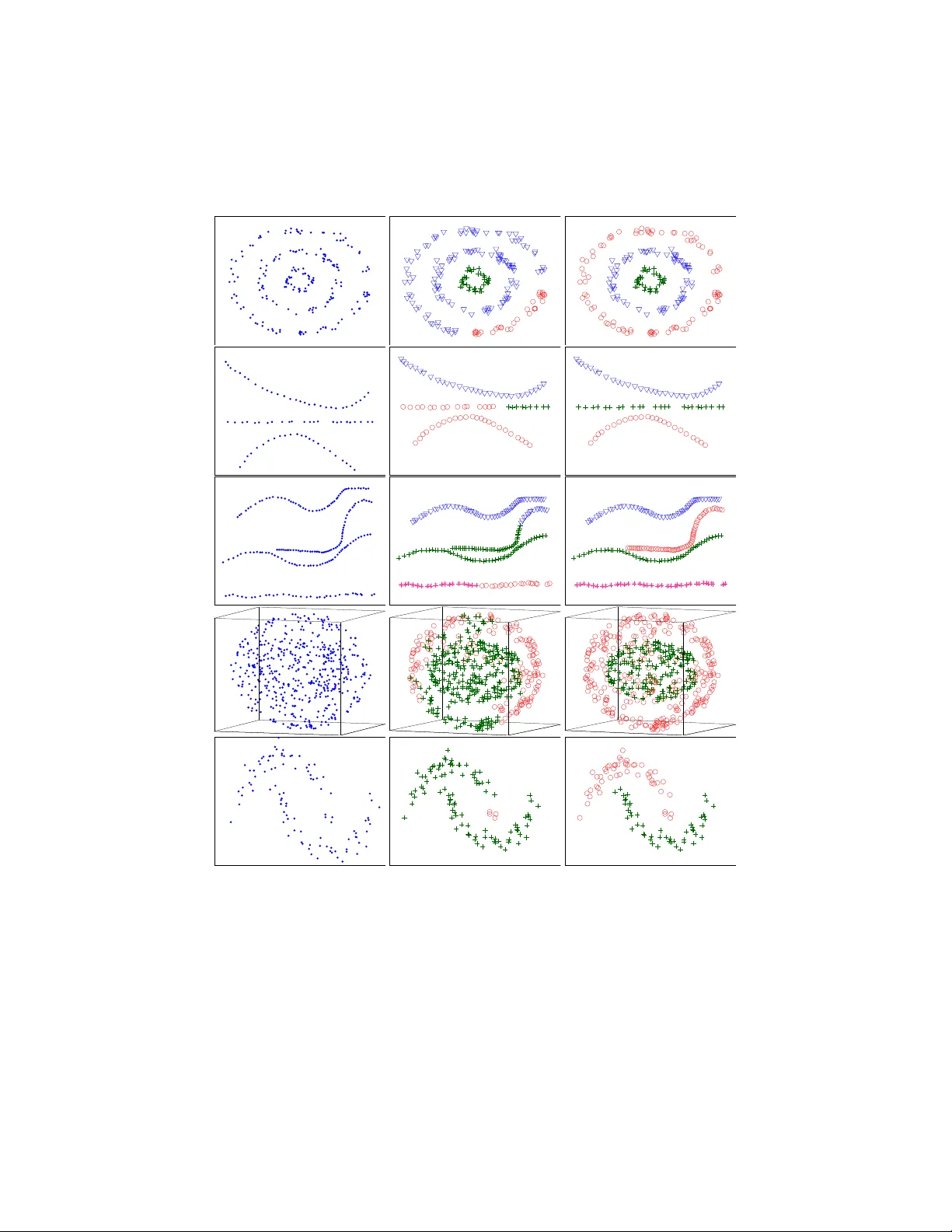
Electronic Journal of Statistics ISSN: 1935-7524 arXiv: stat.ML/1001.1323 Sp ectral Clustering Based on Lo cal Linear Appro ximations Ery Arias-Castro ∗ , Dep artment of Mathematics, University of California, San Die go, e-mail: eariasca@ucsd.edu and Guangliang Chen , Dep artment of Mathematics, Duke University, e-mail: glchen@math.duke.edu and Gilad Lerman , Dep artment of Mathematics, University of Minnesota, Twin Cities, e-mail: lerman@umn.edu Abstract: In the context of clustering, we assume a generativ e mo del where each cluster is the result of sampling points in the neighborho od of an embedded smooth surface; the sample may b e con taminated with outliers, which are modeled as points sampled in space a wa y from the clusters. W e consider a protot yp e for a higher-order spectral clustering metho d based on the residual from a lo cal linear approximation. W e obtain theoretical guarantees for this algorithm and show that, in terms of b oth separation and robustness to outliers, it outperforms the standard spectral clustering algorithm (based on pairwise distances) of Ng, Jordan and W eiss (NIPS ’01). The optimal choice for some of the tuning parameters depends on the dimension and thic kness of the clusters. W e pro vide estimators that come close enough for our theoretical purp oses. W e also discuss the cases of clus- ters of mixed dimensions and of clusters that are generated from smo other surfaces. In our exp eriments, this algorithm is sho wn to outperform pairwise spectral clustering on b oth simulated and real data. AMS 2000 sub ject classiﬁcations: 62H30, 62G20; 68T10. Keyw ords and phrases: Sp ectral clustering; Higher-order aﬃnities; Lo- cal linear approximation; Lo cal polynomial approximation; Detection of clusters in point clouds; Dimension estimation; Nearest-neighbor search. 1. In tro duction In a n umber of mo dern applications, the data appear to cluster near some low- dimensional structures. In the particular setting of manifold learning [ 51 , 47 , 7 , 22 , 17 ], the data are assumed to lie near manifolds em b edded in Euclidean space. When m ultiple manifolds are presen t, the foremost task is separating them, meaning the recov ery of the diﬀerent comp onen ts of the data asso ciated with ∗ corresponding author 1 imsart-ejs ver. 2011/11/15 file: higher-order-ejs-112811.tex date: October 23, 2018 Arias-Castr o, Chen and L erman/Higher Order Sp e ctral Clustering 2 the diﬀeren t manifolds. Manifold clustering naturally occurs in the h uman visual cortex, which excels at grouping p oints into clusters of v arious shap es [ 41 , 21 ]. It is also relev an t for a n um b er of mo dern applications. F or example, in cos- mology , galaxies seem to cluster forming v arious geometric structures such as one-dimensional ﬁlamen ts and tw o-dimensional w alls [ 52 , 39 ]. In motion segmen- tation, feature vectors extracted from moving ob jects and track ed along diﬀeren t views cluster along aﬃne or algebraic surfaces [ 35 , 23 , 53 , 10 ]. In face recognition, images of faces in ﬁxed pose under v arying illumination conditions cluster near lo w-dimensional aﬃne subspaces [ 31 , 6 , 19 ], or along lo w-dimensional manifolds when introducing additional p oses and camera views. In the last few years sev eral algorithms for multi-manifold clustering w ere in tro duced; we discuss them individually in Section 1.3.3 . W e focus here on sp ectral clustering metho ds, and in particular, study a protot ypical m ultiw ay metho d relying on lo cal linear appro ximations, with precursors appearing in [ 12 , 1 , 48 , 2 , 27 ]. W e refer to this method as Higher-Order Sp ectral Clustering (HOSC). W e establish theoretical guarantees for this metho d within a standard mathematical framew ork for multi-manifold clustering. Compared with all other algorithms we are a ware of, HOSC is able to separate clusters that are muc h closer together; equiv alently , HOSC is accurate under muc h low er sampling rate than an y other algorithm we kno w of. Roughly sp eaking, a typical algorithm for m ulti-manifold clustering relies on lo cal characteristics of the p oint cloud in a w a y that presupp oses that all p oints, or at least the v ast ma jority of the p oin ts, in a (small enough) neighborho o d are from a single cluster, except in places lik e in tersections of clusters. In contrast, though HOSC is also a lo cal metho d, it can work with neigh b orho o ds where tw o or more clusters co exist. 1.1. Higher-Or der Sp e ctr al Clustering (HOSC) W e introduce our higher-order spectral clustering algorithm in this section, trac- ing its origins to the sp ectral clustering algorithm of Ng et al. [ 42 ] and the sp ectral curv ature clustering of Chen and Lerman [ 12 , 11 ]. Sp ectral metho ds are based on building a neighborho o d graph on the data p oin ts and partitioning the graph using its Laplacian [ 22 , 34 ], which is closely related to the extraction of connected comp onents. The version in tro duced by Ng et al. [ 42 ] is an em blematic example—we refer to this approac h as SC. It uses an aﬃnit y based on pairwise distances. Giv en a scale parameter  > 0 and a kernel φ , deﬁne α ( x 1 , x 2 ) =  φ ( k x 1 − x 2 k / ) , x 1 6 = x 2 ; 0 , x 1 = x 2 . (1) ( k · k denotes the Euclidean norm.) Standard c hoices include the heat kernel φ ( s ) = exp( − s 2 ) and the simple kernel φ ( s ) = 1 {| s | < 1 } . Let x 1 , . . . , x N ∈ R D denote the data p oints. SC starts by computing all pairwise aﬃnities W = ( W ij ), with W ij = α ( x i , x j ), for i, j = 1 , . . . , N . It then computes the matrix Z = ( Z ij ) : Z ij = W ij / ( D i D j ) 1 / 2 , where D i = P 1 ≤ j ≤ N W ij is the degree of imsart-ejs ver. 2011/11/15 file: higher-order-ejs-112811.tex date: October 23, 2018 Arias-Castr o, Chen and L erman/Higher Or der Sp ectr al Clustering 3 the i th point in the graph with similarit y matrix W . Note that I − Z is the corresp onding normalized Laplacian. Providing the algorithm with the num b er of clusters K , SC con tinues b y extracting the top K eigen vectors of Z , obtaining a matrix U ∈ R N × K , and after normalizing its ro ws, uses them to embed the data in to R K . The algorithm concludes by applying K -means to the embedded p oin ts. See Algorithm 1 for a summary . Algorithm 1 Sp ectral Clustering (SC) [ 42 ] Input: x 1 , x 2 , ..., x N : the data points  : the aﬃnity scale K : the num b er of clusters Output: A partition of the data into K disjoint clusters Steps: 1: Compute the aﬃnity matrix W = ( W ij ), with W ij = α ( x i , x j ). 2: Compute the Z = ( Z ij ) : Z ij = W ij / ( D i D j ) 1 / 2 , where D i = P j W ij . 3: Extract U = [ u 1 , . . . , u K ], the top K eigenv ectors of Z . 4: Renormalize each row of U to hav e unit norm, obtaining a matrix V . 5: Apply K -means to the row v ectors of V in R K to ﬁnd K clusters. 6: Accordingly group the original p oints into K disjoint clusters. Sp ectral methods utilizing m ultiwa y aﬃnities w ere prop osed to better exploit additional structure presen t in the data. The spectral curv ature clustering (SCC) algorithm of Chen and Lerman [ 12 , 11 ] w as designed for the case of h ybrid linear mo deling where the manifolds are assumed to b e aﬃne, a setting that arises in motion segmen tation [ 35 ]. Assuming that the subspaces are all of dimension d — a parameter of the algorithm, SCC starts b y computing the (p olar) curv ature of all ( d + 2)-tuples, creating an N ⊗ ( d +2) -tensor. The tensor is then ﬂattened in to a matrix A whose product with its transpose, W = AA 0 , is used as an aﬃnit y matrix for the sp ectral algorithm SC. (In practice, the algorithm is randomized for computational tractabilit y .) Kernel spectral curv ature clustering (KSCC) [ 10 ] is a kernel version of SCC designed for the case of algebraic surfaces. The SCC algorithm (and therefore KSCC) is not lo calized in space as it ﬁts a parametric mo del that is global in nature. The metho d w e study here ma y b e seen as a lo calization of SCC, which is appropriate in our nonparametric setting since the manifolds resemble aﬃne surfaces lo cally . This type of approach is men tioned in publications on aﬃnity tensors [ 1 , 48 , 2 , 27 ] and is studied here for the ﬁrst time, to our knowledge. As discussed in Section 4 , all reasonable v arian ts ha ve similar theoretical prop erties, so that we choose one of the simplest v ersions to ease the exp osition. Concretely , we consider a m ultiwa y aﬃnit y that com bines pairwise distances b etw een nearest neighbors and the residual from the b est d -dimensional local linear appro ximation. F ormally , giv en a set of m ≥ d + 2 p oin ts, x 1 , . . . , x m , deﬁne Λ d ( x 1 , . . . , x m ) = min L ∈A d max j =1 ,...,m dist( x j , L ) , (2) where dist( x , S ) := inf s ∈ S k x − s k for a subset S ⊂ R D and A d denotes the set imsart-ejs ver. 2011/11/15 file: higher-order-ejs-112811.tex date: October 23, 2018 Arias-Castr o, Chen and L erman/Higher Or der Sp ectr al Clustering 4 of d -dimensional aﬃne subspaces in R D . In other words, Λ d ( x 1 , . . . , x m ) is the width of the thinnest tub e (or band) around a d -dimensional aﬃne subspace that con tains x 1 , . . . , x m . (In our implemen tation, w e use the mean-square error; see Section 3 .) Given scale parameters  > η > 0 and a kernel function φ , deﬁne the follo wing aﬃnit y: α d ( x 1 , . . . , x m ) = 0 if x 1 , . . . , x m are not distinct; otherwise: α d ( x 1 , . . . , x m ) = φ  diam( x 1 , . . . , x m )   · φ  Λ d ( x 1 , . . . , x m ) η  , (3) where diam( x 1 , . . . , x m ) is the diameter of { x 1 , . . . , x m } . See Figure 1 for an illustration. Fig 1: The circle is of radius / 2 and the band is of half-width η . Assuming we use the simple kernel, the m -tuple on the left has aﬃnity α d equal to one, while the other t wo m -tuples hav e aﬃnity equal to zero, the ﬁrst one for having a diameter exceeding  and the second one for b eing ‘thick er’ than η . Giv en data points x 1 , . . . , x N and approximation dimension d , w e compute all m -w ay aﬃnities, and then obtain pairwise similarities b y clique expansion [ 2 ] (note that several other options are p ossible [ 12 , 48 , 27 ]): W ij = X i 1 ,...,i m − 2 α d ( x i , x j , x i 1 , . . . , x i m − 2 ) . (4) Though it is tempting to c ho ose m equal to d + 2, a larger m allows for more tolerance to weak separation and small sampling rate. The down side is what app ears to b e an impractical computational burden, since the mere computation of W in ( 4 ) requires order O ( N m ) ﬂops. In Section 1.4 , w e discuss ho w to reduce the computational complexit y to O ( N 1+ o (1) ) ﬂops, essentially without compromising p erformance. Once the aﬃnit y matrix W is computed, the SC algorithm is applied. W e call the resulting pro cedure higher-order sp ectral clustering (HOSC), summarized in Algorithm 2 . Note that HOSC is (essen tially) equiv alent to SC when η ≥  , and equiv alen t to SCC when  = ∞ . imsart-ejs ver. 2011/11/15 file: higher-order-ejs-112811.tex date: October 23, 2018 Arias-Castr o, Chen and L erman/Higher Or der Sp ectr al Clustering 5 Algorithm 2 Higher Order Sp ectral Clustering (HOSC) Input: x 1 , x 2 , ..., x N : the data points d, m : the appro ximation dimension and aﬃnity order , η : the aﬃnity scales K : the num b er of clusters Output: A partition of the data into K disjoint clusters Steps: 1: Compute the aﬃnity matrix W = ( W ij ) according to ( 4 ). 2: Apply SC (Algorithm 1 ). 1.2. Gener ative Mo del It is time to in tro duce our framework. W e assume a generativ e mo del where the clusters are the result of sampling p oints near surfaces em b edded in an ambien t Euclidean space, sp eciﬁcally , the D -dimensional unit hypercub e (0 , 1) D . F or a surface S ⊂ (0 , 1) D and τ > 0, deﬁne its τ -neighborho o d as B ( S , τ ) = { x ∈ (0 , 1) D : dist( x , S ) < τ } . The reach of S is the supremum ov er τ > 0 such that, for each x ∈ B ( S, τ ), there is a unique p oint realizing inf {k x − s k : s ∈ S } [ 20 ]. It is well-kno wn that, for C 2 submanifolds, the reach b ounds the radius of curv ature from be- lo w [ 20 , Lem. 4.17]. F or a connection to computational geometry , the reach coincides with the condition num b er introduced in [ 43 ] for submanifolds with- out b oundary . Let vol d ( S ) denote the d -dimensional Hausdorﬀ measure, and ∂ S the b oundary of S within (0 , 1) D . F or an in teger 1 ≤ d ≤ D − 1 and a constant κ ≥ 1, let S 2 d ( κ ) b e the class of d -dimensional, connected, C 2 submanifolds S ⊂ (0 , 1) D of 1 /κ ≤ diam( S ) ≤ κ and reach( S ) ≥ 1 /κ , and if S has a b ound- ary , ∂ S is a ( d − 1)-dimensional C 2 submanifold with reach( ∂ S ) ≥ 1 /κ . Given surfaces S 1 , . . . , S K ∈ S 2 d ( κ ) and τ < 1 /κ , w e generate clusters X 1 , . . . , X K b y sampling N k p oin ts uniformly at random in B ( S k , τ ), the τ -neigh b orho o d of S k in (0 , 1) D , for all k = 1 , . . . , K . W e call τ the jitter level. Except for Section 2.3 , where we allow for in tersections, we assume that the surfaces are separated b y a distance of at least δ ≥ 0, i.e. dist( S k , S ` ) := inf x ∈ S k inf y ∈ S ` k x − y k ≥ δ, ∀ k 6 = `. (5) In that case, b y the triangle inequalit y , the actual clusters are separated by at least δ − 2 τ , i.e. dist( X k , X ` ) ≥ δ − 2 τ . W e assume that the clusters are comparable in size b y requiring that N k ≤ ζ N ` for all k 6 = ` , for some ﬁnite constant ζ . Let x 1 , . . . , x N denote the data p oints th us generated. See Figure 2 for an illustration. Giv en data X := { x 1 , . . . , x N } , we aim at recov ering the clusters X 1 , . . . , X K . F ormally , a clustering algorithm is a function taking data X , and p ossibly other imsart-ejs ver. 2011/11/15 file: higher-order-ejs-112811.tex date: October 23, 2018 Arias-Castr o, Chen and L erman/Higher Or der Sp ectr al Clustering 6 Fig 2: This ﬁgure illustrates the generative mo del. Left: Three surfaces (here curves) with their τ -neighborho o d. The curves are separated by at least δ . Righ t: Poin ts sam- pled within the tubular neighborho o ds of the surfaces. tuning parameters, and outputs a partition of X . W e sa y that it is ‘perfectly accurate’ if the output partition coincides with the original partition of X into X 1 , . . . , X K . Our main fo cus is on relating the sample size N and the separation requiremen t in ( 5 ) (in order for HOSC to cluster correctly), and in particular w e let τ and δ v ary with N . This dep endency is left implicit. In con trast, we assume that d, K, ζ are ﬁxed. Also, w e assume that d, τ , K are kno wn throughout the pap er (except for Section 2.1 where we consider their estimation). Though our setting is already quite general, we discuss some imp ortant extensions in Section 4 . W e will also consider the situation where outliers may be present in the data. By outliers w e mean p oin ts that w ere not sampled near any of the underlying surfaces. W e consider a simple mo del where outliers are p oints sampled uni- formly in (0 , 1) D \ S k B ( S k , δ 0 ) for some δ 0 > 0, in general diﬀerent from δ . That is, outliers are at least a distance δ 0 a w ay from the surfaces. W e let N 0 denote the num b er of outliers, while N still denotes the total n umber of data p oin ts, including outliers. See Figure 3 for an illustration. 1.3. Performanc e in terms of Sep ar ation and R obustness 1.3.1. Performanc e of SC A n um b er of pap ers analyze SC under generativ e mo dels similar to ours [ 3 , 54 , 44 , 40 ], and the closely related metho d of extracting connected comp onen ts of the neighborho o d graph [ 3 , 37 , 9 , 36 ]. The latter necessitates a compactly sup- p orted kernel φ and may b e implemen ted via a union-of-balls estimator for the imsart-ejs ver. 2011/11/15 file: higher-order-ejs-112811.tex date: October 23, 2018 Arias-Castr o, Chen and L erman/Higher Or der Sp ectr al Clustering 7 Fig 3: This ﬁgure illustrates the generativ e mo del with outliers included in the data. supp ort of the densit y [ 16 ]. Under the weak er (essentially Lipschitz) regularity assumption C − 1  d ≤ v ol d ( B ( s ,  ) ∩ S ) ≤ C  d , ∀  ∈ (0 , 1 /C ) , ∀ s ∈ S, (6) Arias-Castro [ 3 ] shows that SC with a compactly supp orted kernel is accurate if δ − 2 τ  sep N :=  log N N  1 /d ∨ τ 1 − d/D  log N N  1 /D . (7) ( a ∨ b denotes the maxim um of a and b and a N  b N if a N /b N → ∞ as N → ∞ ). With the heat k ernel, the same result holds up to a √ log N multiplicativ e factor. See also [ 37 , 36 ], whic h prov e a similar result for the metho d of extracting connected components under stronger regularit y assumptions. At the v ery least, ( 7 ) is necessary for the union-of-balls approach and for SC with a compactly supp orted kernel, because sep N is the order of magnitude of the largest distance b et w een a p oint and its closest neigh b or from the same cluster [ 45 ]. Note that ( 6 ) is v ery natural in the con text of clustering as it preven ts S from b eing to o narrow in some places and p ossibly confused with t wo or more disconnected surfaces. And, when C in ( 6 ) is large enough and κ is small enough, it is satisﬁed b y an y surface S b elonging to S 2 d ( κ ). Indeed, suc h a surface resem bles an aﬃne subspace lo cally and ( 6 ) is obviously satisﬁed for an aﬃne surface. When outliers ma y b e presen t in the data, as a prepro cessing step, we iden tify as outliers data p oints with low connectivity in the graph with aﬃnity matrix W , and remov e these p oints from the data b efore pro ceeding with clustering. (This is done b etw een Steps 1 and 2 in Algorithm 1 .) In the con text of spectral imsart-ejs ver. 2011/11/15 file: higher-order-ejs-112811.tex date: October 23, 2018 Arias-Castr o, Chen and L erman/Higher Or der Sp ectr al Clustering 8 clustering, this is very natural; see, e.g., [ 12 , 37 , 3 ]. Using the pairwise aﬃnity ( 1 ), outliers are prop erly iden tiﬁed if δ 0 − τ satisﬁes the low er bound in ( 7 ) and if the sampling is dense enough, sp eciﬁcally [ 3 ], N k ≥ ( N d/D ∨ N τ D − d ) log ( N ) , ∀ k = 1 , . . . , K. (8) When the surfaces are only required to b e of Lipsc hitz regularit y as in ( 6 ), we are not aw are of any metho d that can ev en detect the presence of clusters among outliers if the sampling is substantially sparser. 1.3.2. Performanc e of HOSC Metho ds using higher-order aﬃnities are obviously more complex than metho ds based solely on pairwise aﬃnities. Indeed, HOSC dep ends on more parame- ters and is computationally more demanding than SC. One, therefore, wonders whether this higher level of complexity is justiﬁed. W e show that HOSC do es impro v e on SC in terms of clustering p erformance, b oth in terms of required separation b etw een clusters and in terms of robustness to outliers. Our main con tribution in this pap er is to establish a separation requirement for HOSC whic h is substan tially weak er than ( 7 ) when the jitter τ is small enough. Sp eciﬁcally , HOSC op erates under the separation δ − 2 τ  ( τ ∧ sep N ) ∨ sep 2 N , (9) where a ∧ b denotes the minim um of a and b , and sep N is the separation re- quired for SC with a compactly supp orted k ernel, deﬁned in ( 7 ). This is prov ed in Theorem 1 of Section 2 . In particular, in the jitterless case (i.e. τ = 0), the magnitude of the separation required for HOSC is (roughly) the square of that for SC at the same sample size; equiv alently , at a given separation, HOSC re- quires (roughly) the square ro ot of the sample size needed by SC to correctly iden tify the clusters. 0 0.2 0.4 0.6 0.8 1 0 0.1 0.2 0.3 0.4 0.5 0.6 0.7 0.8 0.9 1 Fig 4: Left: data. Middle: output from SC. Right: output from HOSC. The sampling is muc h sparser than in the original pap er of Ng et al. [ 42 ], which is why SC fails. This ﬁgure is part of Figure 13 in Section 3 , which displays more n umerical exp erimen ts. That HOSC requires less separation than SC is also observed n umerically . In Figure 4 w e compare the outputs of SC and HOSC on the emblematic example imsart-ejs ver. 2011/11/15 file: higher-order-ejs-112811.tex date: October 23, 2018 Arias-Castr o, Chen and L erman/Higher Or der Sp ectr al Clustering 9 of concen tric circles given in [ 42 ] (here with three circles). While the former fails completely , the latter is p erfectly accurate. Indeed, SC requires that the ma jority of points in an  -ball around a giv en data p oin t come from the cluster con taining that point. In con trast, HOSC is able to prop erly operate in situations where the separation betw een clusters is so small, or the sampling rate is so low, that any suc h neigh b orho o d is empt y of data points except for the one point at the cen ter. T o further illustrate this point, consider the simplest p ossible setting consisting of t w o parallel line segments in dimension D = 2, separated by a distance δ > 0, sp eciﬁcally , S 1 := { ( t, 0) : t ∈ [0 , 1] } and S 2 := { ( t, δ ) : t ∈ [0 , 1] } . Supp ose N / 2 p oin ts are sampled uniformly on eac h of these line segments. It is well-kno wn that the t ypical distance b et w een a p oin t on S k and its nearest neigh b or on S k is of order O (1 / N ); see [ 45 ]. Hence, a method computing lo cal statistics requires neigh b orho o ds of radius at least of order 1 / N , for otherwise some neigh b orho o ds are empty . F rom ( 9 ), HOSC is p erfectly accurate when δ = (log N ) 3 / N 2 , say . When the separation δ is that small, t ypical ball of radius of order 1 / N around a data p oin t con tains ab out as many points from S 1 as from S 2 (th us SC cannot w ork). See Figure 5 for an illustration. 0 1 0 5 x 10 −3 0 1 0 5 x 10 −3 Fig 5: Clustering results obtained by SC (left) and HOSC (right) on a data set of tw o lines with small separation ( δ = 0 . 005). 100 p oints are sampled from each line, equally spaced (at a distance 0 . 01). Note that the inter-point separation on the same cluster is twice as large as the separation b etw een clusters. In this case, SC cannot separate the tw o lines correctly , as we ha ve argued. In contrast, HOSC performs p erfectly when clustering the data, which again agrees with the theory and our exp ectation. W e ha ve also tried increasing the separation δ from 0 . 005 to 0 . 025, in whic h case both SC and HOSC perform correctly . As a bonus, w e also sho w that HOSC is able to resolve intersections in some (v ery) special cases, while SC is incapable of that. See Prop osition 6 and also Figure 12 . T o mak e HOSC robust to outliers, w e do exactly as describ ed ab ov e, iden- tifying outliers as data p oints with lo w connectivity in the graph with aﬃnit y matrix W , this time computed using the multiw ay aﬃnity ( 3 ). The separation and sampling requirements are substan tially weak er than ( 8 ), sp eciﬁcally , δ 0 − τ imsart-ejs ver. 2011/11/15 file: higher-order-ejs-112811.tex date: October 23, 2018 Arias-Castr o, Chen and L erman/Higher Or der Sp ectr al Clustering 10 is required to satisfy the low er b ound in ( 9 ) and the sampling N k  ( N d/ (2 D − d ) ∨ N τ D − d ) log ( N ) , ∀ k = 1 , . . . , K. (10) This is established in Prop osition 5 , and again, w e are not aw are of an y metho d for detection that is reliable when the sampling is substantially sparser. F or example, when τ = 0 and we are clustering curv es ( d = 1) in the plane ( D = 2) (with background outliers), the sampling requirement in ( 8 ) is roughly N k  N 1 / 2 log( N ), compared to N k  N 1 / 3 log( N ) in ( 10 ). In Figure 6 b elow we compare b oth SC and HOSC on outliers detection, using the data in Figure 4 but further corrupted with 33 . 3% outliers. 0 0.2 0.4 0.6 0.8 1 0 0.1 0.2 0.3 0.4 0.5 0.6 0.7 0.8 0.9 1 Fig 6: Left: data with outliers. Middle: outliers (black dots) detected by SC. Right: outliers (blac k dots) detected by HOSC. This ﬁgure is part of Figure 15 in Section 3 , where more outliers-remov al experiments are conducted. 1.3.3. Other Metho ds W e focus on comparing HOSC and SC to make a strong p oint that higher-order metho ds ma y b e preferred to simple pairwise metho ds when the underlying clusters are smooth and the jitter level is small. In fact, w e believe that no metho d suggested in the literature is able to comp ete with HOSC in terms of separation requirements. W e quickly argue why . The algorithm of Kushnir et al. [ 32 ] is m ultiscale in nature and is rather complex, incorp orating lo cal information (density , dimension and principal di- rections) within a soft sp ectral clustering approach. In the con text of semi- sup ervised learning, Goldb erg et al. [ 25 ] in tro duce a sp ectral clustering metho d based on a lo cal principal comp onents analysis (PCA) to utilize the unlab eled p oin ts. Both metho ds rely on lo cal PCA to estimate the lo cal geometry of the data and they b oth operate by coarsening the data, even tually applying sp ec- tral clustering to a small subset of p oints acting as representativ e hubs for other p oin ts in their neighborho o ds. They b oth implicitly require that, for the most part, the v ast ma jority of data points in eac h neigh b orho o d where the statistics are computed come from a single cluster. Souvenir and Pless [ 49 ] suggest an al- gorithm that starts with ISOMAP and then alternates in EM-fashion b etw een the cluster assignmen t and the computation of the distances betw een p oints and clusters—this is done in a lo w er dimensional Euclidean space using an MDS em- b edding. Though this iterativ e metho d app ears very c hallenging to be analyzed, imsart-ejs ver. 2011/11/15 file: higher-order-ejs-112811.tex date: October 23, 2018 Arias-Castr o, Chen and L erman/Higher Or der Sp ectr al Clustering 11 it relies on pairwise distances computed as a prepro cessing step to deriv e the geo desic distances, which implicitly assumes that the p oints in small enough neigh b orho o ds are from the same manifold. Thus, like the SC algorithm, all these methods eﬀectively rely on neighborho o ds where only one cluster dom- inates. This is strong evidence that their separation requirements are at best similar to that of SC. The metho ds of Haro et al. [ 30 ] and Gionis et al. [ 24 ] are solely based on the lo cal dimension and density , and are p ow erless when the underlying manifolds are of same dimension and sampled more or less uni- formly , which is the fo cus of this pap er. The metho d of Guo et al. [ 29 ] relies on minimizing an energy that, just as HOSC, incorp orates the diameter and lo cal curv ature of m -tuples, with m = 3 for curves and m = 4 for surfaces in 3D, and the minimization is combinatorial ov er the cluster assignment. In principle, this metho d could b e analyzed with the arguments w e deplo y here. That said, it seems computationally intractable. 1.4. Computational Consider ations Th us it appears that HOSC is superior to SC and other metho ds in terms of separation b etw een clusters and robustness to outliers, when the clusters are smo oth and the jitter is small. But is HOSC even computationally tractable? Assume K and D are ﬁxed. The algorithm starts with building the neigh- b orho o d graph (i.e., computing the matrix W ). This may b e done by brute force in O ( mN m ) ﬂops. Clearly , this ﬁrst step is prohibitive, in particular since w e recommend using a (mo derately) large m . Ho wev er, w e may restrict com- putations to p oints within distance  , which essentially corresp onds to using a compactly supported kernel φ . Hence, we could apply a range search algorithm to reduce computations. Alternatively , at each point we ma y restrict computa- tions to its ` = ω N log( N ) nearest neighbors, with ω N → ∞ , or in a slightly diﬀeren t fashion, adapt the local scaling metho d proposed in [ 56 ] b y replac- ing  in α d ( x i 1 , . . . , x i m ) by (  i 1 · · ·  i m ) 1 /m , where  i denotes the distance b e- t w een x i and its ` th nearest neighbor. The reason is that the central condition ( 12 ) eﬀectiv ely requires that the degree at each p oint be of order log( N ) m − 1 (roughly), which is guaranteed if the ` -nearest neighbors are included in the computations; see [ 3 , 36 ] for rigorous arguments leading to that conclusion. In lo w dimensions, D = O (log log N ), a range search and ` -nearest-neighbor searc h may be computed eﬀectiv ely with kd-trees in O ( N p oly(log N )) ﬂops. In higher dimensions, it is essen tial to use metho ds that adapt to the in trinsic dimensionalit y of the data. Assuming that d is small, the method suggested in [ 8 ] has a similar computational complexity . Hence, the (approximate) aﬃnit y matrix W can b e computed in order O ( N p oly(log N )) + O ( N · ` m ); assuming m ≤ log( N ) / ( ω N log log( N )), this is of order O ( N 1+1 /ω N ). This is within the p ossible choices for m in Theorem 1 . Assume we use the ` -nearest-neighbor approximation to the neighborho o d graph, with ` = ω N log( N ). Then computing Z may b e done in O ( N 1+1 /ω N ) ﬂops, since the aﬃnity matrix W has at most ` m = O ( N 1 /ω N ) non-zero co eﬃ- cien ts p er ro w. Then extracting the leading K eigen vectors of Z ma y be done in imsart-ejs ver. 2011/11/15 file: higher-order-ejs-112811.tex date: October 23, 2018 Arias-Castr o, Chen and L erman/Higher Or der Sp ectr al Clustering 12 O ( K N 1+1 /ω N ) ﬂops, using Lanczos-type algorithms [ 15 ]. Thus w e may run the ` -nearest neigh b or v ersion of HOSC in O ( N 1+1 /ω N ) ﬂops, and it ma y be shown to p erform comparably . W e actually implemen ted the ` -nearest-neigh b or v ariant of HOSC and tried it on a num b er of simulated datasets and a real dataset from motion segmen tation. The results are presen ted in Section 3 . The code is publicly av ailable online [ 13 ]. 1.5. Content The rest of the pap er is organized as follo ws. The main theoretical results are in Section 2 where we pro vide theoretical guaran tees for HOSC, including in con texts where outliers are presen t or the underlying clusters intersect. W e em- phasize that HOSC is only able to separate intersecting clusters under very stringen t assumptions. In the same section w e also address the issue of estimat- ing the parameters that need to b e pro vided to HOSC. In theory at least, they ma y b e c hosen automatically . In Section 3 we implemented our own version of HOSC and rep ort on some n umerical exp eriments in v olving both simulated and real data. Section 4 discusses a num b er of imp ortant extensions, suc h as when the surfaces self-in tersect or hav e b oundaries, which are excluded from the main discussion for simplicity . W e also discuss the case of manifolds of diﬀeren t in- trinsic dimensions, suggesting an approac h that runs HOSC multiple times with diﬀeren t d . And we describe a k ernel v ersion of HOSC that could tak e adv antage of higher degrees of smo othness. Other extensions are also men tioned, including the use of diﬀerent k ernels. The pro ofs are p ostp oned to the App endix. 2. Theoretical Guaran tees Our main result pro vides conditions under whic h HOSC is p erfectly accurate with probability tending to one in the framew ork introduced in Section 1.2 . Throughout the pap er, we state and pro v e our results when the surfaces ha v e no b oundary and for the simple kernel φ ( s ) = 1 {| s | < 1 } , for conv enience and ease of exposition. W e discuss the case of surfaces with boundaries in Section 4.2 and the use of other k ernels in Section 4.5 . Theorem 1. Consider the gener ative mo del of Se ction 1.2 . F or ρ N → ∞ slow ly (e.g., ρ N = log log N ), assume the p ar ameters of HOSC satisfy log N ≥ m ≥ log N √ log ρ N , (11)  ≥  ρ 2 N log N N  1 /d ∨ τ 1 − d/D  ρ 2 N log N N  1 /D . (12) and η ≥  ∧ ( τ + ρ N  2 ) (13) imsart-ejs ver. 2011/11/15 file: higher-order-ejs-112811.tex date: October 23, 2018 Arias-Castr o, Chen and L erman/Higher Or der Sp ectr al Clustering 13 Assume that ( 5 ) holds with δ − 2 τ >  ∧ ρ N η . (14) Under these c onditions, when N is lar ge enough, HOSC is p erfe ctly ac cur ate with pr ob ability at le ast 1 − N − ρ N . T o relate this to the separation requirement stated in the Introduction, the condition ( 9 ) is obtained from ( 14 ) b y choosing  and η equal to their resp ective lo w er b ounds in ( 12 ) and ( 13 ). W e further comment on the theorem. First, the result holds if ρ N = ρ and ρ is suﬃcien tly large. W e state and prov e the result when ρ N → ∞ as a matter of conv enience. Also, by ( 11 ) and ( 14 ), the w eak est separation requirement is ac hiev ed when m is at least of order sligh tly less than O (log N ) so that ρ N is of order O (1). Ho wev er, as discussed in Section 1.4 , the algorithm is not computationally tractable unless m = o (log N ). This is another reason why w e fo cus on the case where ρ N → ∞ . Regarding the constrain ts ( 12 )-( 13 ) on  and η , they are there to guaran tee that, with probabilit y tending to one, eac h cluster is ‘strongly’ connected in the neighborho o d graph. Note that the b ound on  is essen tially the same as that required b y the pairwise sp ectral metho d SC [ 3 , 36 ]. In turn, once each cluster is ‘strongly’ connected in the graph, clusters are assumed to b e separated enough that they are ‘weakly’ connected in the graph. The low er b ound ( 14 ) quantiﬁes the required separation for that to happ en. Note that it is speciﬁc to the simple k ernel. F or example, the heat k ernel would require a multiplicativ e factor prop ortional to √ log N . So how do es HOSC compare with SC? When the jitter is large enough that τ  (log( N ) / N ) 1 /d , we ha ve η ≥  and the lo cal linear appro ximation contribu- tion to ( 3 ) do es not come into pla y . In that case, the tw o algorithms will output the same clustering (see Figure 7 for an example). 0 1 −0.01 0 0.01 0.02 0.03 0 1 −0.01 0 0.01 0.02 0.03 Fig 7: Clustering results obtained by SC (left) and HOSC (righ t) on the data set of Figure 5 , but with separation δ = 0 . 025 and jitter τ = 0 . 01. In this example, neither SC nor HOSC can successfully separate the t wo lines. This example supp orts our claim that when the jitter is large enough (relative to separation), HOSC do es not improv e o ver SC and the t wo algorithms will output the same clustering. imsart-ejs ver. 2011/11/15 file: higher-order-ejs-112811.tex date: October 23, 2018 Arias-Castr o, Chen and L erman/Higher Or der Sp ectr al Clustering 14 When the jitter is small enough that τ  (log ( N ) / N ) 1 /d , HOSC requires less separation, as demonstrated in Figure 5 . In tuitively , in this regime the clusters are sampled densely enough relative to the thickness τ that the smo othness of the underlying surfaces comes in to fo cus and eac h cluster, as a p oint cloud, b ecomes locally well-appro ximated b y a thin band. W e pro vide some n umerical exp erimen ts in Section 3 sho wing HOSC outp erforming SC in v arious settings. Th us, HOSC impro v es on SC only when the jitter is small. This condition is quite sev ere, though again, we do not know of any other metho d that can accurately cluster under the weak separation requirement display ed here, even in the jitterless case. It is p ossible that some form of scan statistic (i.e., matc hed ﬁlters) may be able to op erate under the same separation requirement without needing the jitter to b e small, how ever, we do not know ho w to compute it in our nonparametric setting—even in the case of hybrid linear mo deling where the surfaces are aﬃne, computing the scan statistic app ears to b e computationally in tractable. A t any rate, the separation required b y HOSC is essentially optimal when τ is of order O ( N − 1 /d ) or smaller. A quick argumen t for the case d = 1 and D = 2 go es as follows. Consider a line segmen t of length one and sample N p oin ts uniformly at random in its τ -neighborho o d, with τ = O (1 / N ). The claim is that this neigh b orho o d contains an empt y band of thic kness of order slightly less than O (1 / N 2 ), and therefore cannot be distinguished from tw o parallel line segmen ts. Indeed, such band of half-width λ inside that neigh b orho o d is empt y of sample p oin ts with probabilit y (1 − λ/τ ) N , whic h con verges to 1 if N λ/τ → 0, and when τ = O (1 / N ), this is the case if λ = o (1 / N 2 ). In regards to the c hoice of parameters, the recommended c hoices dep end solely on ( d, τ , K ). These mo del c haracteristics are sometimes una v ailable and w e discuss their estimation in Section 2.1 . Afterwards, we discuss issues such as outliers (Section 2.2 ) and in tersection (Section 2.3 ). 2.1. Par ameter Estimation In this section, w e prop ose some metho ds to estimate the intrinsic dimension d of the data, the jitter τ and the num b er of clusters K . Though w e show that these metho ds are consisten t in our setting, further numerical exp eriments are needed to determine their p oten tial in practice. Compared to SC, HOSC requires the sp eciﬁcation of three additional pa- rameters. This is no small issue in practice. In theory , how ever, w e recommend c ho osing d and K consistent with their true v alues,  and η as functions of τ , and m of order slightly less than log ( N ). The true unkno wns are therefore ( d, τ , K ). W e provide estimators for d and K that are consisten t, and an estimator for τ that is accurate enough for our purp oses. Speciﬁcally , we estimate d and τ using the correlation dimension [ 28 ] and an adaptation of our o wn design. The n um b er of clusters K is estimated via the eigengap of the matrix Z . imsart-ejs ver. 2011/11/15 file: higher-order-ejs-112811.tex date: October 23, 2018 Arias-Castr o, Chen and L erman/Higher Or der Sp ectr al Clustering 15 2.1.1. The Intrinsic Dimension and the Jitter L evel A n umber of metho ds hav e b een prop osed to estimate the in trinsic dimensional- it y; w e refer the reader to [ 33 ] and references th erein. The correlation dimension, ﬁrst in tro duced in [ 28 ], is perhaps the most relev ant in our context, since surfaces ma y b e close together. Deﬁne the pairwise correlation function Cor(  ) = X i X j 6 = i 1 {k x i − x j k≤  } . The authors of [ 28 ] recommend plotting log Cor(  ) v ersus log  and estimating the slop e of the linear part. W e use a slightly diﬀerent estimator that allo ws us to estimate τ too, if it is not to o small. The idea is to regress log Cor(  ) on log  and identify a kink in the curve. See Figure 8 for an illustration. −6 −5 −4 −3 −2 −1 0 1 2 3 4 5 6 7 8 9 log( ε ) log(Cor( ε )) Fig 8: A correlation curve for a simulated data set of 240 p oints sampled from the τ -neigh b orho o d of three disjoint one-dimensional curves ( d = 1) in dimension ten ( D = 10) crossing all dimensions. The jitter is τ = 0 . 01. W e see that the linear part of the curv e has slope (near) 1, which coincides with the intrinsic dimension of the curv es. The kink appears near ˆ τ := exp( − 4 . 5) = 0 . 0111, a close appro ximation to τ . Though sev eral (mostly ad ho c) metho ds ha v e been prop osed for ﬁnding kinks, we describ e a simple metho d for which we can prov e consistency . Fix ρ N → ∞ , with ρ N  log N . Deﬁne r N = −  log log( N ) − log N d log ρ N  − 2 . Let A r = log Cor( ρ − r N ). If there is r ∈ { 3 , . . . , r N − 2 D − 1 } suc h that ( A r − A r +1 ) / log ρ N > D − 1 / 2 , then let ˆ r ≥ 0 be the smallest such r ; otherwise, let ˆ r = r N − 2 D . Deﬁne ˆ τ = ρ − ˆ r N ; and also ˆ d = D , if ˆ r = 3, and ˆ d the closest integer to ( A 3 − A ˆ r ) / ( ˆ r log ρ N ), otherwise. imsart-ejs ver. 2011/11/15 file: higher-order-ejs-112811.tex date: October 23, 2018 Arias-Castr o, Chen and L erman/Higher Or der Sp ectr al Clustering 16 Prop osition 1. Consider the gener ative mo del describ e d in Se ction 1.2 with S 1 , . . . , S K ∈ S 2 d ( κ ) . Assume that τ ≤ ρ − 3 N and, if ther e ar e N 0 outliers, assume that N − N 0 ≥ N /ρ N . Then the fol lowing holds with pr ob ability at le ast 1 − N − √ ρ N : if ˆ r < r N − 2 D , then τ ∈ [ ˆ τ /ρ N , ρ N ˆ τ ] ; if ˆ r = r N − 2 D , then τ ≤ ˆ τ ; mor e over, if ˆ r > 3 , ˆ d = d . In the context of Prop osition 1 , the only time that ˆ d is inconsistent is when τ is of order ρ − 3 N or larger, in which case ˆ d = D ; this makes sense, since the region S k B ( S k , τ ) is in fact D -dimensional if τ is of order 1. Also, ˆ τ is within a ρ N factor of τ if τ is not m uc h smaller than (log ( N ) / N ) 1 /d . W e now extend this metho d to deal with a smaller τ . Consider what we just did. The quantit y Cor(  ) is the total degree of the  -neighborho o d graph built in SC. Fixing ( d, m ), we now consider the total degree of the η -neighborho o d graph built in HOSC. Deﬁne the multiw ay correlation function Cor d,m ( , η ) = X i D 1 / ( m − 1) i . Similarly , we shall regress log Cor d,m ( , η ) on log η and iden tify a kink in the curv e (Figure 9 displays suc h a curve). −12 −10 −8 −6 −4 −2 0 1 2 3 4 5 6 7 8 9 log( ε ) log(Cor( ε )) −12 −11 −10 −9 −8 −7 −6 −5 −4 2 3 4 5 log( η ) log(Cor( η )) Fig 9: Correlation curv es corresponding to SC (left) and HOSC (right) for the data set of Figure 8 , but with a muc h smaller τ = 1 e − 4. W e see that the pairwise correlation function w orks p oorly in this case, while the multiw ay correlation curve has a kink near ˆ τ := exp( − 10 . 5) = 2 . 754 e − 5, within a factor of 1 4 of the true τ . Using the multiw ay correlation function, we then prop ose an estimator ˆ τ as follo ws. W e assume that the metho d of Prop osition 1 returned ˆ r = r N − 2 D , for otherwise we know that ˆ τ is accurate. Cho ose d = ˆ d and m ≥ log( N )(log ρ N ) 2 . Note that this is the only time w e require m to b e larger than log N . Let B s = log Cor d,m ( ρ − ˆ r N , ρ − ˆ r − s N ). If there is s ∈ { 0 , . . . , ˆ r − 1 } such that ( B s − B s +1 ) / log ρ N > D − d − 1 / 2 , then let ˆ s be the smallest one; otherwise, let ˆ s = ˆ r . W e then redeﬁne ˆ τ as ˆ τ = ρ − ˆ r − ˆ s +1 N . imsart-ejs ver. 2011/11/15 file: higher-order-ejs-112811.tex date: October 23, 2018 Arias-Castr o, Chen and L erman/Higher Or der Sp ectr al Clustering 17 Prop osition 2. In the c ontext of Pr op osition 1 , assume that ˆ r = r N − 2 D . Then r e deﬁning ˆ τ as done ab ove, the fol lowing holds with pr ob ability at le ast 1 − N − √ ρ N : if ˆ s < ˆ r , then τ ∈ [ ˆ τ /ρ N , ρ N ˆ τ ] ; if ˆ s = ˆ r , then τ ≤ ˆ τ . No w, ˆ τ comes close to τ if τ is not muc h smaller than (log( N ) / N ) 2 /d . Whether this is the case, or not, the statement of Theorem 1 applies with ˆ τ in place of τ in ( 13 ). Though our metho d works in theory , it is deﬁnitely asymptotic. In practice, w e recommend using other approaches for determining the lo cation of the kink and the slop e of the linear part of the pairwise correlation function (in log- log scale). Robust regression methods with high break-do wn p oints, like least median of squares and least trimmed squares, work ed w ell in several examples. W e do not pro vide details here, as this is fairly standard, but the ﬁgures are quite evocative. 2.1.2. The Numb er of Clusters HOSC dep ends on c ho osing the n umber of clusters K appropriately . A common approac h consists in choosing K b y insp ecting the eigenv alues of Z . W e show that, prop erly tuned, this metho d is consistent within our mo del. Prop osition 3. Compute the matrix Z in HOSC with the same choic e of p a- r ameters as in The or em 1 , exc ept that know le dge of K is not ne e de d. Set the numb er of clusters e qual to the numb er of eigenvalues of Z (c ounting multiplic- ity) exc e e ding 1 − N − 2 /ρ N . Then with pr ob ability at le ast 1 − N − ρ N , this metho d cho oses the c orr e ct numb er of clusters. W e implicitly assumed that d and τ are known, or hav e b een estimated as describ ed in the previous section. The pro of of Prop osition 3 is parallel to that of [ 3 , Prop. 4], this time using the estimate provided in part (A1) of the pro of of Theorem 1 . Details are omitted. Figure 10 illustrates a situation where the n umber of clusters is correctly c ho- sen by inspection of the eigenv alues, more sp eciﬁcally , by coun ting the num b er of eigenv alue 1 in the spectrum of Z (up to n umerical error). This success is due to the fact that the clusters are well-separated, and even then, the eigengap is quite small. W e apply this strategy to more data later in Section 3 , and sho w that it can correctly identify the parameter K in some cases (see Figure 14 ). In general w e do not exp ect this metho d to w ork w ell when the data has large noise or in tersecting clusters, though we do not know of any other metho d that works in theory under our v ery weak separation requiremen ts. 2.2. When Outliers ar e Pr esent So far w e hav e only considered the case where the data is devoid of outliers. W e now assume that some outliers may be included in the data as describ ed at imsart-ejs ver. 2011/11/15 file: higher-order-ejs-112811.tex date: October 23, 2018 Arias-Castr o, Chen and L erman/Higher Or der Sp ectr al Clustering 18 1 2 3 4 5 6 0.994 0.995 0.996 0.997 0.998 0.999 1 1.001 Fig 10: The top six eigenv alues of the weigh t matrix Z obtained b y HOSC in Step 2 for the same data used in Figure 8 . Though in this example the clusters are well-separated, the eigengap is still very small (about 0.005). the end of Section 1.2 . As stated there, we lab el as outlier an y data p oint with lo w degree in the neigh b orho o d graph, as suggested in [ 12 , 37 , 3 ]. Sp eciﬁcally , w e compute D as in Step 2 of HOSC, and then lab el as outliers p oin ts x i with degree D i b elo w some threshold. Let ρ N → ∞ slo w er than any p ow er of N , e.g., ρ N = log N . W e prop ose tw o thresholds: (O1) Identify as outliers p oints with degree: D 1 / ( m − 1) i ≤ ρ − 1 N max j D 1 / ( m − 1) j . (O2) Identify as outliers p oints with degree: D 1 / ( m − 1) i ≤ ρ N N  d η D − d . T aking up the task of iden tifying outliers, only the separation betw een outliers and non-outliers is relev ant, so that we do not require an y separation b etw een the actual clusters. W e ﬁrst analyze the p erformance of (O1) , whic h requires ab out the same separation betw een outliers and non-outliers as HOSC requires b et w een p oints from diﬀeren t clusters in ( 14 ). Prop osition 4. Consider the gener ative mo del describ e d in Se ction 1.2 . Assume that N − N 0 ≥ N /ρ N and that ( 11 ) - ( 13 ) hold. In terms of sep ar ation, assume that δ 0 − τ >  ∧ ρ N η . Then with pr ob ability at le ast 1 − N − ρ N , the pr o c e dur e (O1) identiﬁes outliers without err or. W e now analyze the p erformance of (O2) , which requires a stronger separa- tion b etw een outliers and non-outliers, but op erates under very w eak sampling requiremen ts. Prop osition 5. Assume that m is as in ( 11 ) , and  = ( ρ N log( N ) / N ) 1 / (2 D − d ) , η = ( ρ N log( N ) / N ) 2 / (2 D − d ) . (15) imsart-ejs ver. 2011/11/15 file: higher-order-ejs-112811.tex date: October 23, 2018 Arias-Castr o, Chen and L erman/Higher Or der Sp ectr al Clustering 19 In terms of sep ar ation, assume that δ 0 − τ >  . In addition, supp ose that N k ≥ ρ N log( N ) N d/ (2 D − d ) ∨ N τ D − d , ∀ k = 1 , . . . , K. (16) Then with pr ob ability at le ast 1 − N − ρ N , the pr o c e dur e (O2) identiﬁes outliers without err or. If δ 0 = τ , so that outliers are sampled ev erywhere but within the τ -tubular re- gions of the underlying surfaces, then b oth (O1) and (O2) ma y miss some outliers within a short distance from some B ( S k , τ ). Sp eciﬁcally , (O1) (resp. (O2) ) ma y miss outliers within  ∧ ρ N η (resp. within  ) from some B ( S k , τ ). Using W eyl’s tub e formula [ 55 ], we see that there are order N 0 (  ∧ ρ N η ) D − d (resp. N 0  D − d ) suc h outliers, a small fraction of all outliers. The sampling requiremen t ( 16 ) is w eaker than the corresp onding requiremen t for pairwise metho ds display ed in ( 8 ). In fact, ( 16 ) is only sligh tly stronger than what is required to just detect the presence of a cluster hidden in noise. W e brieﬂy explain this p oin t. Instead of clustering, consider the task of detecting the presence of a cluster hidden among a large num b er of outliers. F ormally , w e observe the data x 1 , . . . , x N , and wan t to decide b etw een the follo wing t wo h yp otheses: under the null, the points are independent, uniformly distributed in the unit h yp ercub e (0 , 1) D ; under the alternativ e, there is a surface S 1 ∈ S 2 d ( κ ) suc h that N 1 p oin ts are sampled from B ( S 1 , τ ) as described in Section 1.2 , while the rest of the p oints, N − N 1 of them, are sampled from the unit hypercub e (0 , 1) D , again uniformly . Assuming that the parameters d and τ are known, it is shown in [ 5 , 4 ] that the scan statistic is able to separate the n ull from the alternativ e if N 1  N d/ (2 D − d ) ∨ N τ D − d . (17) W e are not aw are of a metho d that is able to solv e this detection task at a substan tially low er sampling rate, and ( 16 ) comes within a logarithmic factor from ( 17 ). W e thus obtain the remark able result that accurate clustering is p ossible within a log factor of the b est (known) sampling rate that allows for accurate detection in the same setting. 2.3. When Clusters Interse ct W e no w consider the setting where the underlying surfaces ma y intersect. The additional conditions w e introduce are implicit constrain ts on the dimension of, and the incidence angle at, the intersections. W e supp ose there is an integer 0 ≤ d int ≤ d − 1 and a ﬁnite constant C > 0 such that v ol d ( B ( S k ∩ S ` ,  ) ∩ S k ) ≤ C  d − d int , ∀  ∈ (0 , 1 /κ ) , ∀ k 6 = `. (18) (The subscript int stands for ‘in tersection’.) In addition, we assume that for some θ int ∈ (0 , π / 2], dist( x , S ` ) ≥ δ ∧ sin( θ int ) dist( x , S k ∩ S ` ) , ∀ x ∈ S k , ∀ k 6 = ` with S k ∩ S ` 6 = ∅ . (19) imsart-ejs ver. 2011/11/15 file: higher-order-ejs-112811.tex date: October 23, 2018 Arias-Castr o, Chen and L erman/Higher Or der Sp ectr al Clustering 20 ( 18 ) is slightly stronger than requiring that S k ∩ S ` has ﬁnite d int -dimensional v olume. If the surfaces are aﬃne, it is equiv alen t to the condition dim( S k ∩ S ` ) ≤ d int , ∀ k 6 = `. ( 19 ), on the other hand, is a statemen t ab out the minimum an- gle at which any tw o surfaces intersect. F or example, if the surfaces are aﬃne within distance δ of their in tersection, then ( 19 ) is equiv alent to their maxi- m um (principal) angle b eing b ounded from b elow b y θ int . See Figure 11 for an illustration. Fig 11: Illustration of intersecting surfaces. Though the h uman eye easily distinguishes the tw o clusters, the clustering task is a lot harder for machine learning algorithms. The main issue is that there are to o many data p oin ts at the intersection of the tw o tubular regions. How ev er, in v ery sp ecial cases HOSC is able to separate intersecting clusters (see Figure 12 for suc h an example). Prop osition 6. Consider the setting of The or em 1 , with ( 5 ) r eplac e d by ( 19 ). In addition, assume that ( 18 ) holds. Deﬁne γ N := N 2  d (  ∧ ρ N η ) d − d int (sin θ int ) d int − d . Then ther e is a c onstant C > 0 such that, with pr ob ability at le ast 1 − C γ N , HOSC is p erfe ctly ac cur ate. The most fav orable case is when τ = 0 and θ int = π / 2. Then with our choice of  and η in Theorem 1 , assuming ρ N increases slo wly , e.g., ρ N ≺ log N , we ha v e γ N → 0 if 2 d int < d , and partial results suggest this cannot b e impro ved substan tially . This constrain t on the in tersection of t wo surfaces is rather sev ere. Indeed, a t ypical in tersection b etw een t wo (smo oth) surfaces of same dimension d is of dimension d − 1, and if so, only curves satisfy this condition. Figure 12 pro vides a n umerical example sho wing the algorithm successfully separating t w o intersecting one-dimensional clusters. Thus, ev en with no jitter and the surfaces intersecting at right angle, HOSC is only able to separate in tersecting imsart-ejs ver. 2011/11/15 file: higher-order-ejs-112811.tex date: October 23, 2018 Arias-Castr o, Chen and L erman/Higher Or der Sp ectr al Clustering 21 clusters under exceptional circumstances. Moreov er, even when the conditions of Prop osition 6 are fulﬁlled, the probabilit y of success is no longer exp onentially small, but is at b est of order (1 / N ) 1 − 2 d int /d . That said, SC do es not seem able to properly deal with in tersections at all (see also Figure 12 ). It essen tially corresp onds to taking η =  in HOSC, in which case γ N nev er tends to zero. 0 0.2 0.4 0.6 0.8 1 0 0.1 0.2 0.3 0.4 0.5 0.6 0.7 0.8 0.9 1 Fig 12: Left: data. Middle: output from HOSC. Righ t: Output from SC. This example sho ws that HOSC is able to separate intersecting curvilinear clusters when the inci- dence angle is perp endicular and there is no jitter ( τ = 0). In particular, the conditions of Proposition 6 are satisﬁed. On the con trary , SC fails in this case. Though the implications of Prop osition 6 are rather limited, we do not know of an y other clustering metho d which prov ably separates intersecting clusters under a similar generative mo del. This is a ﬁrst small step to w ards ﬁnding such a metho d. 3. Soft ware and Numerical Exp erimen ts W e include in this section a few exp eriments where a preliminary implemen- tation of HOSC outp erforms SC, to demonstrate that higher-order aﬃnities can bring a signiﬁcant improv ement o ver pairwise aﬃnities in the con text of manifold clustering. In our implemen tation of HOSC, we used the heat kernel φ ( s ) = exp( − s 2 ). F ollowing the discussion in Section 1.4 , at each p oint w e restrict the compu- tations to its ` nearest neighbors so that we practically remo ve the lo cality parameter  from the aﬃnit y function of ( 3 ) and obtain α d ( x 1 , . . . , x m ) = ( φ (Λ d ( x 1 , . . . , x m ) /η ) , if x 2 , . . . , x m ∈ ` -NN( x 1 ) distinct; 0 , otherwise , (20) where ` -NN( x 1 ) is the set of the ` nearest neighbors of x 1 . F or computational ease, we used Λ (2) d ( x 1 , . . . , x m ) = min L ∈A d v u u t 1 m m X j =1 dist( x j , L ) 2 , (21) whic h can b e easily computed using the b ottom m − d singular v alues of the m p oints. Note that, since Λ d / √ m ≤ Λ (2) d ≤ Λ d , the results we obtained apply , imsart-ejs ver. 2011/11/15 file: higher-order-ejs-112811.tex date: October 23, 2018 Arias-Castr o, Chen and L erman/Higher Or der Sp ectr al Clustering 22 with η changed by a √ m factor, at most. (In the paper, the standard choice for η is a pow er of N , while m is of order at most log N , so this factor is indeed negligible.) In practice, w e alw a ys search a subin terv al of [0 , 1] for the b est w orking η (e.g., [ . 001 , . 1]), based on the smallest v ariance of the corresp onding clusters in the eigenspace (the ro w space of the matrix V ), as suggested in [ 42 ]. When the giv en data contains outliers, the optimal choice of η is based on the largest gap b etw een the means of the t wo sets of degrees (associated to the inliers and outliers), normalized by the maxim um degree. The co de is av ailable online [ 13 ]. 3.1. Synthetic Data W e ﬁrst generate ﬁv e syn thetic data sets in the unit cub e (0 , 1) D ( D = 2 or 3), sho wn in Figure 13 . In this exp eriment, the actual num b er of clusters (i.e. K ) and dimension of the underlying manifolds (i.e. d ) are assumed known to all algorithms. F or HOSC, we ﬁx ` = 10 , m = d + 2, and use the subinterv al [0 . 001 , 0 . 1] as the searc h in terv al of η . F or SC, w e considered t wo w ays of tuning the scale parameter  : directly , b y choosing a v alue in the int erv al [0 . 001 , 0 . 25] (SC-NJW); and by the lo cal scaling metho d of [ 56 ] (SC-LS), with the num b er of nearest neighbors ` = 5 , . . . , 15. The ﬁnal c hoices of these parameters w ere also based on the same criterion as used b y HOSC. Figure 13 exhibits the clusters found b y each algorithm when applied to the ﬁv e data sets, resp ectiv ely . Observe that HOSC succeeded in a n umber of diﬃcult situations for SC, e.g., when the sampling is sparse, or when the separation is small at some lo cations. W e also plot the leading eigenv alues of the matrix Z obtained by HOSC on eac h data set; see Figure 14 . W e see that in data sets 1, 2, 5, the num b er of eigen v alue 1 coincides with the true num b er of clusters, while in 3 and 4 there is some discrepancy b et w een the K th eigenv alue and the num b er 1. Though we do not expect the eigengap method to work well in general, Figure 14 sho ws that it can b e useful in some cases. Figure 15 displays some exp eriments including outliers. W e simply sampled p oin ts from the unit square (0 , 1) 2 uniformly at random and added them as out- liers to the ﬁrst three data sets in Figure 13 , with p ercen tages 33.3%, 60% and 60%, respectively . W e applied SC and HOSC assuming kno wledge of the propor- tion of outliers, and lab eled p oints with smallest degrees as outliers. Cho osing the threshold automatically remains a challenge; in particular, we did not test the theory . W e observe that HOSC could successfully remo ve most of the true outliers, lea ving out smo oth structures in the data; in con trast, SC tended to k eep isolated high-densit y regions, b eing insensitive to sparse smo oth structures. A h undred replications of this experiment (i.e., ﬁxing the clusters and adding randomly gen- erated outliers) sho w that the T rue Positiv e Rates (i.e., p ercentages of correctly iden tiﬁed outliers) for (SC, HOSC) are (58.1% vs 67.7%), (75.4% vs 86.8%) and (76.8% vs 88.0%), resp ectively . imsart-ejs ver. 2011/11/15 file: higher-order-ejs-112811.tex date: October 23, 2018 Arias-Castr o, Chen and L erman/Higher Or der Sp ectr al Clustering 23 0 0.2 0.4 0.6 0.8 1 0 0.1 0.2 0.3 0.4 0.5 0.6 0.7 0.8 0.9 1 0 0.2 0.4 0.6 0.8 1 0 0.1 0.2 0.3 0.4 0.5 0.6 0.7 0.8 0.9 1 0 0.2 0.4 0.6 0.8 1 0 0.1 0.2 0.3 0.4 0.5 0.6 0.7 0.8 0.9 1 0 0.2 0.4 0.6 0.8 1 0 0.1 0.2 0.3 0.4 0.5 0.6 0.7 0.8 0.9 1 0 0.2 0.4 0.6 0.8 1 0 0.1 0.2 0.3 0.4 0.5 0.6 0.7 0.8 0.9 1 Fig 13: Left column: data. (The third example shows a sphere containing an ellipsoid inside.) Middle column: b est output from SC with the scale parameter chosen by b oth searching the interv al [0 . 001 , 0 . 25] and applying lo cal scaling [ 56 ] with at most 15 nearest neighbors. Right column: output from HOSC. The optimal v alue of η is selected from the interv al [0 . 001 , 0 . 1]. W e also tried the simple kernel instead of the heat k ernel, and obtained same results except in data set 3. imsart-ejs ver. 2011/11/15 file: higher-order-ejs-112811.tex date: October 23, 2018 Arias-Castr o, Chen and L erman/Higher Or der Sp ectr al Clustering 24 1 2 3 4 5 6 0.994 0.995 0.996 0.997 0.998 0.999 1 1.001 1 2 3 4 5 6 0.965 0.97 0.975 0.98 0.985 0.99 0.995 1 1.005 1 2 3 4 5 6 7 0.99 0.992 0.994 0.996 0.998 1 1.002 1 2 3 4 0.985 0.99 0.995 1 1.005 1 2 3 4 0.997 0.998 0.999 1 1.001 Fig 14: T op eigen v alues of the matrix Z obtained by HOSC on each of the ﬁv e data sets in Figure 13 (in same order). 0 0.2 0.4 0.6 0.8 1 0 0.1 0.2 0.3 0.4 0.5 0.6 0.7 0.8 0.9 1 0 0.2 0.4 0.6 0.8 1 0 0.1 0.2 0.3 0.4 0.5 0.6 0.7 0.8 0.9 1 0 0.2 0.4 0.6 0.8 1 0 0.1 0.2 0.3 0.4 0.5 0.6 0.7 0.8 0.9 1 Fig 15: Outlier-remov al experiments. Left column: data with outliers. The percentages of outliers are 33.3%, 60% and 60%, resp ectively . Middle: outliers (blac k dots) detected b y pairwise spectral clustering (b oth SC-NJW and SC-LS, but only the b etter result is shown). Righ t: outliers (black dots) detected b y HOSC. The use of the simple kernel (instead of the heat kernel) in HOSC gives very similar results. imsart-ejs ver. 2011/11/15 file: higher-order-ejs-112811.tex date: October 23, 2018 Arias-Castr o, Chen and L erman/Higher Or der Sp ectr al Clustering 25 3.2. R e al Data W e next compare SC and HOSC using the tw o-view motion data studied in [ 10 , 46 ]. This data set con tains 13 motion sequences: (1) b oxes , (2) c arsnbus3 , (3) deliveryvan , (4) desk , (5) lightbulb , (6) manyc ars , (7) man-in-oﬃc e , (8) nrb o oks3 , (9) oﬃc e , (10) p arking-lot , (11) p osters-che ckerb o ar d , (12) p osters-keyb o ar d , and (13) toys-on-table ; and each sequence consists of tw o image frames of a 3-D dynamic scene taken by a persp ective camera (see Figure 16 for a few such sequences). Supp ose that sev eral feature p oints hav e been extracted from the mo ving ob jects in the t wo camera views of the scene. The task is to separate the tra jectories of the feature p oints according to diﬀerent motions. This applica- tion, which lies in the ﬁeld of structur e fr om motion , is one of the fundamental problems in computer vision. Fig 16: Three exemplary t w o-view motion sequences (arranged in columns): (4) desk , (6) manyc ars and (7) man-in-oﬃc e . The true clusters are displa yed in diﬀerent colors and mark ers (the black dots are outliers). Giv en a physical p oint x ∈ R 3 and its image corresp ondences in the tw o views ( x 1 , y 1 ) 0 , ( x 2 , y 2 ) 0 ∈ R 2 , one can alw ays form a join t image sample y = ( x 1 , y 1 , x 2 , y 2 , 1) 0 ∈ R 5 . It is shown in [ 46 ] that, under p ersp ectiv e camera pro- jection, all the join t image samples y corresp onding to diﬀerent motions liv e on diﬀeren t manifolds in R 5 , some having dimension 2 and others ha ving dimen- sion 4. Exploratory analysis applied to these data suggests that the manifolds in this dataset mostly hav e dimension 2 (see Figure 17 ). Therefore, we will apply our algorithm (HOSC) with d = 2 to these data sets in order to compare with pairwise sp ectral clustering (SC-NJW, SC-LS). W e use the following parameter v alues for the t w o algorithms. In HOSC, we c ho ose ` = 20 , m = d + 2 , η ∈ [ . 0001 , . 1], while in SC we try b oth searching the in terv al [ . 001 , . 5] (SC-NJW) and local scaling with at most 24 nearest neighbors (SC-LS). imsart-ejs ver. 2011/11/15 file: higher-order-ejs-112811.tex date: October 23, 2018 Arias-Castr o, Chen and L erman/Higher Or der Sp ectr al Clustering 26 −1 0 1 −0.4 −0.2 0 0.2 0.4 −0.4 −0.2 0 0.2 0.4 0.6 −1 −0.5 0 0.5 −0.5 0 0.5 −0.1 −0.05 0 0.05 0.1 −0.8 −0.6 −0.4 −0.2 0 0.2 0.4 0.6 −0.5 0 0.5 −0.1 −0.05 0 0.05 0.1 Fig 17: The true clusters of the three sequences in Figure 16 (in same order), shown in top three principal dimensions. (The outliers hav e b een remov ed from the data and th us are not display ed). These plots clearly indicate that the underlying manifolds are t wo dimensional. The original data contains some outliers. In fact, 10 sequences out of the 13 are corrupted with outliers, with the largest percentage b eing ab out 32%. W e ﬁrst manually remov e the outliers from those sequences and solely fo cus on the clustering asp ects of the tw o algorithms. Next, we add outliers bac k and compare them regarding outliers remov al. (Note that we need to provide b oth algorithms with the true p ercentage of outliers in each sequence.) By doing so w e hope to ev aluate the clustering and outliers remo v al aspects of an algorithm separately and thus in the most accurate wa y . T able 1 The misclassiﬁc ation r ates and the numb ers of true outliers dete cte d by HOSC, SC-NJW and SC-LS. In the clustering exp eriment, the outliers-fr e e data is use d; then the outliers ar e adde d b ack so that e ach of these algorithms c an b e applie d to detect them. F or SC-NJW, the tuning p ar ameter is selecte d fr om the interval [ . 001 , . 5] ; for SC-LS, a maximum of 24 ne ar est neighb ors ar e use d; for HOSC, 20 ne ar est neighb ors ar e use d and the ﬂatness p ar ameter η is sele cte d from the interval [ . 0001 , . 1] . Data Clustering Errors # T rue Outliers Detected seq. #samples #out. SC-NJW SC-LS HOSC SC-NJW SC-LS HOSC 1 115,121 2 0.85% 0.85% 0.85% 1 1 1 2 85,45,89 28 0% 0% 0% 24 24 24 3 62,192 0 30.3% 23.6% 30.3% N/A N/A N/A 4 50,50,55 45 0.65% 2.58% 1.29% 35 30 37 5 51,121,33 0 0% 0% 0% N/A N/A N/A 6 54,24,23,43 0 18.8% 0% 0% N/A N/A N/A 7 16,57 34 19.2% 19.2% 0% 17 12 26 8 129,168,91 32 22.9% 17.8% 22.9% 12 17 23 9 76,109,74 48 0% 0% 0% 36 28 36 10 19,117 4 0% 47.8% 0% 0 0 1 11 100,99,81 99 0% 1.79% 0% 42 39 73 12 99,99,99 99 0.34% 0.34% 0% 80 43 91 13 49,42 35 33.0% 15.4% 2.20% 7 6 21 T able 1 presents the results from the experiments abov e. Observe that HOSC ac hiev ed excellen t clustering results in all but t wo sequences, with zero error on eigh t sequences, one mistake on sequence (13), and tw o mistakes on eac h of imsart-ejs ver. 2011/11/15 file: higher-order-ejs-112811.tex date: October 23, 2018 Arias-Castr o, Chen and L erman/Higher Or der Sp ectr al Clustering 27 (1) and (4). W e remark that HOSC also outp erformed the algorithms in [ 10 , T able 1], in terms of clustering accuracy , but due to the main aim of this pap er, w e do not include those results in T able 1 . In contrast, each of SC-NJW and SC-LS failed on at least ﬁve sequences (with ov er 15% misclassiﬁcation rates), b oth containing the tw o bad sequences for HOSC. As a sp eciﬁc example, we displa y in Figure 18 the clusters obtained by b oth HOSC and SC on sequence (7), demonstrating again that higher order aﬃnities can signiﬁcantly improv e o v er pairwise aﬃnities in the case of manifold data. Regarding outliers remov al, HOSC is also consistently b etter than SC-NJW and SC-LS (if not equally goo d). −0.8 −0.6 −0.4 −0.2 0 0.2 0.4 0.6 −0.5 0 0.5 −0.1 −0.05 0 0.05 0.1 −0.8 −0.6 −0.4 −0.2 0 0.2 0.4 0.6 −0.5 0 0.5 −0.1 −0.05 0 0.05 0.1 Fig 18: Clustering results of b oth HOSC and SC (left to right) on sequence (7). (The truth is shown in Figure 17 , righ tmost plot). In this example, HOSC correctly found the t wo clusters, using geometric information; in contrast, SC failed b ecause it solely relies on pairwise distances. 4. Extensions 4.1. When the Underlying Surfac es Self-Interse ct In our generativ e model described in Section 1.2 w e assume that the surfaces are submanifolds, implying that they do not self-intersect. This is really for con v enience as there is essen tially no additional diﬃcult y arising from self- in tersections. If w e allo w the surfaces to self-intersect, then we b ound the maxi- m um curv ature (from abov e) and not the reach. W e could, for example, consider surfaces of the form S = f ( B d (0 , 1)), where f : B d (0 , 1) → (0 , 1) D is lo cally bi- Lipsc hitz and has bounded second deriv ative. A similar model is considered in [ 38 ] in the context of set estimation. Clearly , proving that each cluster is connected in the neigh b orho o d graph in this case is the same. The only issue is in situations where a surface comes within distance  from another surface at a lo cation where the latter in tersects itself. The geometry in v olv ed in suc h a situation is indeed complex. If w e p ostulate that no such situation arises, then our results generalize immediately to this setting. imsart-ejs ver. 2011/11/15 file: higher-order-ejs-112811.tex date: October 23, 2018 Arias-Castr o, Chen and L erman/Higher Or der Sp ectr al Clustering 28 4.2. When the Underlying Surfac es Have Boundaries When the surfaces hav e b oundaries, points near the b oundary of a surface may b e substantially connected with points on a nearb y surface. See Figure 19 for an illustration. This is symptomatic of the fact that the algorithm is not able to resolve in tersections in general, as discussed in Section 2.3 , with the notable exception of clusters of dimension d = 1, as illustrated in the ‘t wo mo ons’ example of Figure 13 . Fig 19: An example of a surface with a b oundary coming close to another surface. This is a p otentially problematic situation for HOSC as the points near the boundary of one surface and close to the other surface may be strongly connected to p oints from b oth clusters. Numerically , w e sho w in Figure 13 such an example where HOSC is successful. If we require a stronger separation b etw een the b oundary of a surface and the other surfaces, sp eciﬁcally , dist( ∂ S k , S ` ) ≥ δ ‡ , ∀ k 6 = `, (22) with δ ‡ − 2 τ >  , no p oin t near the b oundary of a cluster is close to a point from a diﬀeren t cluster. (A corresp onding requirement in the con text of outliers w ould b e that outliers b e separated from the b oundary of a cluster by at least δ 0 , ‡ , with δ 0 , ‡ − τ >  .) 4.3. When the Data is of Mixe d Dimensions In a num b er of situations, the surfaces ma y b e of diﬀeren t in trinsic dimensions. An imp ortant instance of that is the study of the distribution of galaxies in space, where the galaxies are seen to cluster along ﬁlaments ( d = 1) and walls imsart-ejs ver. 2011/11/15 file: higher-order-ejs-112811.tex date: October 23, 2018 Arias-Castr o, Chen and L erman/Higher Or der Sp ectr al Clustering 29 ( d = 2) [ 39 ]. W e prop ose a top-do wn approac h, implemen ting HOSC for each dimension d starting at D − 1 and ending at 1 (or b etw een any kno wn upper and low er b ounds for d ). A t each step, the algorithm is run on each cluster obtained from the pre- vious step, including the set of p oints identiﬁed as outliers. Indeed, when the dimension parameter of the algorithm is set larger than the dimension of the underlying surfaces, HOSC may not b e able to prop erly separate clusters. F or example, tw o parallel segments satisfying the separation requirement of Theo- rem 1 still b elong to a same plane and HOSC with dimension parameter d = 2 w ould not be able to separate the tw o line segmen ts. Another reason for process- ing the outlier bin is the greater disparity in the degrees of the data p oints in the neighborho o d graph often observ ed with clusters of diﬀeren t dimensions. At eac h step, the num b er of clusters is determined automatically according to the pro cedure describ ed in Section 2.1 , for such information is usually not a v ailable. The parameters  and η are c hosen according to ( 15 ). Partial results suggest that, under some additional sampling conditions, this top-down pro cedure is accurate under w eaker separation requirements than required b y pairwise metho ds, which handle the case of mixed dimensions seamlessly [ 3 ]. The key is that an actual cluster X k , as deﬁned in Section 1.2 , is nev er cut in to pieces. Indeed, prop erties (A1) and (A4) in the pro of of Theorem 1 , which guaran tee the connectivit y and regularit y (in te rms of comparable degrees) of the subgraph represen ted by X k , are easily seen to also b e v alid when the dimension parameter of the algorithm is set larger than d . (This observ ation might explain the success of the SCC algorithm of [ 12 ] in some mixed settings when using an upp er b ound on the in trinsic dimensions.) 4.4. Clustering Base d on L o c al Polynomial Appr oximations F or 1 ≤ d ≤ D − 1 and an in teger r ≥ 3, let S r d ( κ ) b e the sub class of S 2 d ( κ ) of d -dimensional submanifolds S such that, for ev ery x ∈ S with tangen t T x , the orthogonal pro jection S ∩ B ( x , 1 /κ ) → T x is a C r -diﬀeomorphism with all partial deriv atives of order up to r b ounded in supnorm b y κ . F or example, S r d ( κ ) includes a subclass of surfaces of the form S = f ( B d (0 , 1)), where f : B d (0 , 1) → (0 , 1) D is locally bi-Lipschitz and has its ﬁrst r deriv atives b ounded. (W e could also consider surfaces of in termediate, i.e., H¨ older smo othness, a p opular mo del in function and set estimation [ 18 , 38 ].) Giv en that surfaces in S r d are well-appro ximated lo cally by p olynomial sur- faces, it is natural to choose an aﬃnity based on the residual of the b est d - dimensional p olynomial approximation of degree at most r − 1 to a set of p oin ts x 1 , . . . , x m . This ma y b e implemen ted via the “k ernel tric k” with a p olynomial k ernel, as done in [ 10 ] for the sp ecial case of algebraic surfaces. The main dif- ference with the case of C 2 surfaces that we consider in the rest of the pap er is the degree of approximation to a surface S ∈ S r d b y its osculating algebraic surface of order r − 1; within a ball of radius  , it is of order O (  r ). P artial results suggest that, under similar conditions, the k ernel version of HOSC with r kno wn ma y b e able to op erate under a separation of the form imsart-ejs ver. 2011/11/15 file: higher-order-ejs-112811.tex date: October 23, 2018 Arias-Castr o, Chen and L erman/Higher Or der Sp ectr al Clustering 30 ( 9 ), with the exp onent 2 /d replaced by r /d and, in the presence of outliers, within a logarithmic factor of the b est known sampling rate ratio achiev ed b y an y detection metho d [ 5 , 4 ]: min k N k ≥ N d/ ( rD − ( r − 1) d ) ∨ N τ D − d . (23) Regarding the estimation of τ , deﬁning the correlation dimension using the underlying aﬃnit y deﬁned here allo ws to estimate τ accurately do wn to (essen- tially) (log( N ) / N ) r/d , if the surfaces are all in S r d ( κ ). The arguments are parallel and we omit the details. Th us, using the underlying aﬃnity deﬁned here ma y allo w for higher ac- curacy , if the surfaces are smo oth enough. Ho wev er, this comes with a larger computational burden and at the expense of introducing a new parameter r , whic h would need to be estimated if unknown, and w e do not kno w a go o d w ay to do that. 4.5. Other Extensions The setting we considered in this pap er, introduced in Section 1.2 , w as delib- erately more constrained than needed for clarity of exp osition. W e list a few generalizations b elow, all straigh tforward extensions of our work. • Sampling. Instead of the uniform distribution, w e could use any other distribution with a densit y b ounded a wa y from 0 and ∞ , or with fast deca ying tails such as the normal distribution. • Kernel. The rate of decay of the kernel φ dictates the range of the aﬃnity ( 3 ). Let ω N b e a non-decreasing sequence such that N 3 m φ ( ω N ) → 0 . F or a compactly supported k ernel, ω N = sup { s : φ ( s ) > 0 } , while for the heat kernel, we can take ω N = 2 √ m log N . As w e will take m → ∞ , φ is essen tially supp orted in [0 , ω N ] so that p oin ts that are further than ω N  apart ha ve basically zero aﬃnit y . Speciﬁcally , w e use the follo wing b ounds: φ (1) 1 {| s | < 1 } ≤ φ ( s ) ≤ 1 {| s | <ω N } + φ ( ω N ) . The results are identical, except that statemen ts of the form δ − 2 τ > Z are replaced with δ − 2 τ > ω N Z . • Me asur e of ﬂatness. As p oin ted out in the introduction, any reasonable measure of linear appro ximation could b e used instead. Our c hoice was driv en by con venience and simplicit y . App endix A: Preliminaries W e gather here some preliminary results. Recall that, for a, b ∈ R , a ∨ b := max( a, b ); a ∧ b := min( a, b ); a + = a ∨ 0. F or ( a N ) , ( b N ) ∈ R N , a N ≺ b N means a N = O ( b N ); a N  b N means b oth a N = O ( b N ) and b N = O ( a N ); a N  b N means a N = o ( b N ). F or L ∈ A d , P L denotes the orthogonal pro jection onto L . The canonical basis of R D is denoted e 1 , . . . , e D . imsart-ejs ver. 2011/11/15 file: higher-order-ejs-112811.tex date: October 23, 2018 Arias-Castr o, Chen and L erman/Higher Or der Sp ectr al Clustering 31 A.1. L ar ge Deviations Bounds The follo wing result is a simple consequence of Hoeﬀding’s or Bernstein’s in- equalities. Lemma 1 ([ 50 ], Lem. 5.3.7) . L et ( X i ) i ≥ 1 b e indep endent r andom variables in [0 , 1] . If 4 a ≤ P i E ( X i ) , P X i X i ≤ a ! ≤ exp( − a ) . If a ≥ 8 P i E ( X i ) , P X i X i ≥ a ! ≤ exp( − a ) . A.2. Some Ge ometric al R esults W e start b y quantifying how well a surface S ∈ S 2 ( κ ) is lo cally approximated b y its tangen t. Recall that, for an aﬃne subspace T , P T denotes the orthogonal pro jection onto T . F or any s ∈ S , let T s denote the tangent of S at s . Lemma 2. F or any S ∈ S 2 d ( κ ) and s ∈ S , the ortho gonal pr oje ction onto T s is inje ctive on B ( s , 1 / (4 κ )) ∩ S and P − 1 T s has Lipschitz c onstant b ounde d by √ 2 on its image, which c ontains B ( s , 1 / (8 κ )) ∩ T s . Mor e over, B ( s ,  ) ∩ S ⊂ B ( T s , κ 2 ) , ∀ , and B ( s ,  ) ∩ T s ⊂ B ( S, 2 κ 2 ) , ∀  < 1 / (8 κ ) . Pr o of. This sort of result is standard in diﬀerential geometry . W e follow the exp osition in [ 43 ]. W e note that the manifold parameter τ in [ 43 ], i.e., the in v erse of the condition num b e r, coincides with the manifold’s reach. W e thus ﬁx here an S ∈ S 2 d ( κ ) and denote τ := reac h( S ). Since 1 /κ is a lo w er b ound on the reach for manifolds in S 2 d ( κ ), we ha ve the inequalit y τ ≥ 1 /κ . Fix also a p oint s ∈ S . Applying [ 43 , Lem. 5.4], we obtain that P T s is one- to-one on B ( s ,  ) ∩ S for an y  < τ / 2, in particular,  < 1 / (2 κ ). W e obtain an estimate on the image of P T s as follows. W e note that [ 43 , pro of of Lem. 5.3] implies that P T s ( B ( s ,  ) ∩ S ) ⊇ B ( s ,  cos arcsin( / (2 τ ))) ∩ T s . (24) F urthermore, if  ≤ 1 / (4 κ ) , cos arcsin( / (2 τ )) ≥ cos arcsin( κ/ 2) ≥ p 63 / 64 > 1 / 2 . (25) imsart-ejs ver. 2011/11/15 file: higher-order-ejs-112811.tex date: October 23, 2018 Arias-Castr o, Chen and L erman/Higher Or der Sp ectr al Clustering 32 Com bining ( 24 ) and ( 25 ), we conclude that P T s ( B ( s ,  ) ∩ S ) ⊇ B ( s , / 2) ∩ T s , ∀  ≤ 1 / (4 κ ) . (26) In particular, for  = 1 / (4 κ ), we obtain that the range of P T s (when applied to B ( s , 1 / (4 κ )) ∩ S ) contains the ball B ( s , 1 / (8 κ )) ∩ T s . Next, for any s 0 ∈ B ( s , 1 / (4 κ )) ∩ S , the deriv ative of the linear op erator P T s in the direction u , a unit vector in T s 0 , is ∇ u ( P T s ) = ( P T s ) · u = cos θ 1 ( T s , span { u } ) ≥ cos θ 1 ( T s , T s 0 ) , (27) where θ 1 denotes the largest principal angle b etw een the corresp onding sub- spaces. In order to further b ound from b elow the RHS of ( 27 ), w e couple [ 43 , Props. 6.2, 6.3] and use τ ≥ 1 /κ to obtain that cos θ 1 ( T s , T s 0 ) ≥ p 1 − 2 κ k s − s 0 k . (28) Com bining ( 27 ) and ( 28 ) we conclude that P − 1 T s has Lipschitz constan t b ounded b y √ 2 in B ( s , 1 / (4 κ )) ∩ T s . F or the inclusions, we use the fact that k P T s ( x ) − x k ≤ ( κ/ 2) · k s − x k 2 , ∀ x , s ∈ S, (29) whic h app ears in [ 20 , Th. 4.18(2)]. This immediately implies the ﬁrst inclusion— whic h actually holds for any  > 0 and with κ replaced b y κ/ 2. The second inclusion follows b y combining ( 26 ) with ( 29 ). Next, w e estimate the volume of the in tersection of the neighborho o d of a surface and a ball cen tered at a p oint within that neighborho o d. Lemma 3 ([ 3 ], Lem. 1) . F or S satisfying ( 6 ), x ∈ B ( S, τ ) and , τ > 0 , v ol D ( B ( S , τ ) ∩ B ( x ,  ))   d (  ∧ τ ) D − d , vol D ( B ( S , τ ))  τ D − d . The following result is on the approximation of a set of p oin ts in the neigh- b orho o d of a d -dimensional aﬃne subspace by a d -dimensional aﬃne subspace generated by a subset of d + 1 p oints. Lemma 4. Ther e is a c onstant C > 0 dep ending only on d such that, if z 1 , . . . , z m ∈ B ( L, η ) , with L ∈ A d and m ≥ d + 2 , then ther e exists H ∈ A d gener ate d by d + 1 p oints among z 1 , . . . , z m , such that z 1 , . . . , z m ∈ B ( H , C η ) . Pr o of. F or p oints a 1 , . . . , a k , let aspan { a 1 , . . . , a k } denote the aﬃne subspace of minim um dimension passing through a 1 , . . . , a k . Let ( i 1 , i 2 ) ∈ argmax i,j k z i − z j k and, for d ≥ k ≥ 3, i k ∈ arg max i 6 = i 1 ,...,i k − 1 dist( z i , aspan { z i 1 , . . . , z i k − 1 } ) . Let A k = aspan { z i 1 , . . . , z i k +1 } , for d ≥ k ≥ 1. Deﬁne λ 1 = k z i 2 − z i 1 k and, for d ≥ k ≥ 2, λ k = dist( z i k +1 , span { z i 1 , . . . , z i k } ). Also, let v 1 = ( z i 2 − z i 1 ) /λ 1 and, imsart-ejs ver. 2011/11/15 file: higher-order-ejs-112811.tex date: October 23, 2018 Arias-Castr o, Chen and L erman/Higher Or der Sp ectr al Clustering 33 for k ≥ 2, v k = ( z i k +1 − P A k − 1 z i k +1 ) /λ k . Without loss of generalit y , assume that z i 1 is the origin, which allows us to iden tify a p oint z with the v ector z − z i 1 . T ake z ∈ { z 1 , . . . , z m } and express it as z = a 1 v 1 + · · · + a d v d + w , with w ⊥ A d . W e sho w that k w k ≤ C η for a constan t C depending only on d , which implies that z ∈ B ( A d , C η ). Let C 1 > 0, to be made suﬃcien tly large later. By construction, A 1 ⊂ · · · ⊂ A d and λ 1 ≥ · · · ≥ λ d with k P A ⊥ k − 1 z k ≤ λ k for all k = 1 , . . . , d . Consequen tly , if λ d ≤ C 1 η , then k w k ≤ k P A ⊥ d − 1 z k ≤ λ d ≤ C 1 η and w e are done. Therefore, assume that λ d > C 1 η . Deﬁne q k = P L v k . W e hav e k q k − v k k = k P L ⊥ v k k = 1 λ k k P L ⊥ P A ⊥ k − 1 z i k +1 k ≤ 1 λ k k P L ⊥ z i k +1 k ≤ η λ k ≤ 1 C 1 . Hence, for C 1 large enough, q 1 , . . . , q d are linearly indep endent, and therefore span L . Suppose this is the case and deﬁne matrices V with columns v 1 , . . . , v d and Q with columns q 1 , . . . , q d . Then, by con tinuit y , for C 1 large enough we ha v e k P L − P A d k = k Q ( Q T Q ) − 1 Q T − VV T k ≤ 1 / 2 , where k · k here denotes the (Euclidean) op erator norm. When C 1 is that large, w e hav e k P L w k = k ( P L − P A d ) w k ≤ 1 2 k w k ≤ 1 2 ( k P L w k + k P L ⊥ w k ) , so that k P L w k ≤ k P L ⊥ w k . Now, using the triangle inequality , k P L ⊥ w k ≤ k P L ⊥ z k + | a 1 |k P L ⊥ v 1 k + · · · + | a d |k P L ⊥ v d k . (30) Because z ∈ B ( L, η ), we hav e k P L ⊥ z k ≤ η . F or the other terms, w e ha ve k P L ⊥ v k k ≤ η /λ k as before, and, using the fact that, b y construction, the v 1 , . . . , v d are orthonormal with A k = span { v 1 , . . . , v k } and k P A ⊥ k − 1 z k ≤ λ k , together with the Cauch y-Sch wartz inequalit y , w e also hav e | a k | = | v T k z | =    v T k P A ⊥ k − 1 z    ≤ λ k . Hence, the RHS in ( 30 ) is b ounded by ( d + 1) η , implying k w k ≤ k P L w k + k P L ⊥ w k ≤ 2 k P L ⊥ w k ≤ 2( d + 1) η . W e then let C = max( C 1 , 2 d + 2). Belo w w e pro vide an upp er bound on the v olume of the three-w ay intersection of the neighborho o d of a surface, a ball centered at a p oint on the surface and the neigh b orho o d of an aﬃne d -dimensional subspace passing through that p oint, in terms of the angle b et w een this subspace and the tangent to the surface at that same p oint. The principal angles b etw een linear subspaces L, L 0 ∈ A d , denoted b y π 2 ≥ θ 1 ( L, L 0 ) ≥ · · · ≥ θ d ( L, L 0 ) ≥ 0 , imsart-ejs ver. 2011/11/15 file: higher-order-ejs-112811.tex date: October 23, 2018 Arias-Castr o, Chen and L erman/Higher Or der Sp ectr al Clustering 34 are recursively deﬁned as follo ws: cos θ r ( L, L 0 ) = min u ∈ L min u 0 ∈ L 0 u T u 0 = u T r u 0 r , sub ject to k u k = k u 0 k = 1; u T u s = 0 , ∀ s = 1 , . . . , r − 1; u 0 T u 0 s = 0 , ∀ s = 1 , . . . , r − 1 . Note that the orthogonality constrain ts are void when r = 1. (Some authors use the reverse ordering, e.g, [ 26 ].) Lemma 5. Consider a surfac e S ∈ S 2 d ( κ ) . Supp ose  ≥ η ∨ τ , η ≥  2 and τ > 0 . L et Ψ b e the uniform distribution on B ( S, τ ) . F or s ∈ S , let T s b e the tangent sp ac e to S at s . Then for L ∈ A d c ontaining s , Ψ( B ( s ,  ) ∩ B ( L, η )) ≺  d (1 ∧ ( η/τ )) D − d d Y j =1  1 ∧ η ∨ τ  θ j ( L, T s )  . Pr o of. Fix s ∈ S and L ∈ A d con taining s , and let T := T s and θ j := θ j ( L, T ) for short. By deﬁnition, Ψ( B ( s ,  ) ∩ B ( L, η )) = v ol D ( B ( S , τ ) ∩ B ( s ,  ) ∩ B ( L, η )) v ol D ( B ( S , τ )) . By Lemma 3 , it suﬃces to show that v ol D ( B ( S , τ ) ∩ B ( L, η ) ∩ B ( s ,  )) ≺  d ( η ∧ τ ) D − d d Y j =1  1 ∧ η ∨ τ  θ j  . W e divide the pro of into tw o cases; though the proof is similar for b oth, the ﬁrst case is simpler and allo ws us to introduce the main ideas with ease b efore generalizing to the second case. Case  2 ≤ τ . W e use Lemma 2 and the fact that τ ≥  2 , to get B ( S , τ ) ∩ B ( s ,  ) ⊂ B ( T , (1 + κ ) τ ) ∩ B ( s ,  ) . (31) Ignoring the constant factor 1 + κ , w e b ound v ol D ( B ( T , τ ) ∩ B ( L, η ) ∩ B ( s ,  )) . W e may assume without loss of generality that s is the origin and T = span { e 1 , . . . , e d } , and L = span { (cos θ 1 ) e 1 + (sin θ 1 ) e d +1 , . . . , (cos θ d ) e d + (sin θ d ) e 2 d } . imsart-ejs ver. 2011/11/15 file: higher-order-ejs-112811.tex date: October 23, 2018 Arias-Castr o, Chen and L erman/Higher Or der Sp ectr al Clustering 35 Then B ( T , τ ) = { ( z 1 , . . . , z D ) : X j >d z 2 j ≤ τ 2 } ; B ( L, η ) = { ( z 1 , . . . , z D ) : X j ≤ d ( z j sin θ j − z d + j cos θ j ) 2 + X j > 2 d z 2 j ≤ η 2 } ; B ( s ,  ) = { ( z 1 , . . . , z D ) : X j z 2 j ≤  2 } . T ake j ≤ d ; since | z d + j | ≤ τ , we ha ve | z j sin θ j − z d + j cos θ j | ≤ η ⇒ | z j | ≤ 2( η ∨ τ ) / sin θ j ≤ π ( η ∨ τ ) /θ j . Therefore, B ( T , τ ) ∩ B ( L, η ) ∩ B ( s ,  ) ⊂ d Y j =1  −  ∧ π ( η ∨ τ ) θ j ,  ∧ π ( η ∨ τ ) θ j  × B D − d (0 , η ∧ τ ) . F rom that we obtain the desired b ound. Case τ ≤  2 . The arguments here are a little diﬀerent and we simply b ound v ol D ( B ( S , τ ) ∩ B ( s ,  )) . Assume that  < 1 / (8 κ ). Because P T is contractile, w e ha v e P T ( S ∩ B ( s ,  )) ⊂ T ∩ B ( s ,  ) = B d (0 ,  ) , so that, by Lemma 2 , S ∩ B ( s ,  ) ⊂ P − 1 T ( B d (0 ,  )) , where P − 1 T : B d (0 ,  ) → S ∩ B ( s,  ). Hence, B ( S , τ ) ∩ B ( s ,  ) ⊂ { ( a , b ) : a ∈ B d (0 ,  ) , k b − P − 1 T ( a ) k ≤ τ } . And by direct integration, the set on the RHS has D -volume of order  d τ D − d since P − 1 T is Lipschitz on B d (0 ,  ) by Lemma 2 . A companion of the previous result, the following lemma pro vides a low er b ound on the angle b etw een the aﬃne subspace and the tangent. Lemma 6. L et , η > 0 , and take S ∈ S 2 d ( κ ) . Supp ose L ∈ A d is such that B ( L, η ) c ontains s ∈ S and y ∈ B ( s ,  ) . L et T s the tangent to S at s . Then θ 1 ( L, T s ) ≥ dist( y , S ) − 2 κ 2 − η  + η . Pr o of. Let T denote T s for short, and let L 0 b e the line passing through s and P L ( y ). Since L 0 ⊂ L , w e hav e θ 1 ( L, T ) ≥ θ 1 ( L 0 , T ), and using the triangle inequalit y and the fact that θ ≥ sin θ , for θ ≥ 0, this is b ounded b elo w by dist( P L ( y ) , T ) dist( P L ( y ) , s ) ≥ dist( y , T ) − η dist( s , y ) + η . imsart-ejs ver. 2011/11/15 file: higher-order-ejs-112811.tex date: October 23, 2018 Arias-Castr o, Chen and L erman/Higher Or der Sp ectr al Clustering 36 The denominator do es not exceed  + η . F or the n umerator, dist( y , T ) = k P T ( y ) − y k ≥ dist( y , S ) − dist( P T ( y ) , S ) . Since k y − s k ≤  , we ha ve P T ( y ) ∈ T ∩ B ( s ,  ), so that dist( P T ( y ) , S ) ≤ 2 κ 2 b y Lemma 2 . Consequently , the numerator is b ounded from b elow by dist( y , S ) − κ 2 − η . Next is another result estimating some volume intersections. It is similar to Lemma 5 , though the conditions are diﬀerent. Lemma 7. Consider a surfac e S ∈ S 2 d ( κ ) . L et Ψ b e the uniform distribution on B ( S, τ ) . Then for  ≥ η and τ > 0 , sup y ,L Ψ( B ( y ,  ) ∩ B ( L, η )) ≺  d (1 ∧ ( η/τ )) D − d , wher e the supr emum is over y ∈ R D and L ∈ A d , and the implicit c onstants dep end only on κ, d . Also, for  ≥ 10 η , η ≥ 10 κ 2 and τ > 0 , and any x ∈ B ( S , τ ) , sup L Ψ( B ( x ,  ) ∩ B ( L, η ))   d (1 ∧ ( η/τ )) D − d . Pr o of. The pro of is similar to that of Lemma 5 . W e divide the pro of in to tw o parts. Upp er b ound. Let x ∈ B ( S, τ ) ∩ B ( y ,  ) ∩ B ( L, η ). When η ≥ τ , we use B ( S , τ ) ∩ B ( y ,  ) ∩ B ( L, η ) ⊂ B ( S, τ ) ∩ B ( x , 2  ) , while, when η ≤ τ , we use B ( S , τ ) ∩ B ( y ,  ) ∩ B ( L, η ) ⊂ B ( L, η ) ∩ B ( x , 2  ) . In b oth cases, we conclude with Lemma 3 . L ower b ound. Let s b e the point on S closest to x , with tangent subspace T . When η ≥ 2 τ + 4 κ 2 , tak e as L the translate of T passing through x and use Lemma 2 to get B ( S , τ ) ∩ B ( x ,  ) ⊂ B ( T , τ + κ ( τ +  ) 2 ) ⊂ B ( L, η ) , and therefore B ( S , τ ) ∩ B ( x ,  ) ∩ B ( L, η ) ⊃ B ( S, τ ) ∩ B ( x ,  ) . W e then use Lemma 3 . No w, supp ose η ≤ 2 τ + 4 κ 2 and notice that, since η ≥ 10 κ 2 , w e hav e τ ≥ 3 κ 2 . First, assume that  ≥ 10 τ . W e use Lemma 2 to get B ( S , τ ) ∩ B ( x ,  ) ⊃ B ( T , τ − 2 κ 2 ) ∩ B ( s ,  ) ∩ B ( x ,  ) , and therefore, B ( S , τ ) ∩ B ( x ,  ) ∩ B ( L, η ) ⊃ B ( T , τ − 2 κ 2 ) ∩ B ( L, η ) ∩ B ( s ,  ) ∩ B ( x ,  ) . (32) imsart-ejs ver. 2011/11/15 file: higher-order-ejs-112811.tex date: October 23, 2018 Arias-Castr o, Chen and L erman/Higher Or der Sp ectr al Clustering 37 Without loss of generality , assume that x is the origin, L = span { e 1 , . . . , e d } . Since the v olume is least when k x − s k = τ , assume that s = τ e d +1 (seen as a point in space). Deﬁne ν = ( η + 2 κ 2 ) / 2 and note that ν ≤ η ∧ (2 τ ) b y the conditions on η and τ . Then B ( T , τ − 2 κ 2 ) ∩ B ( L, η ) ⊃ { ( z 1 , . . . , z D ) : X j >d +1 z 2 j + ( z d +1 − ν ) 2 ≤ ( η / 3) 2 } ; B ( s ,  ) = { ( z 1 , . . . , z D ) : X j 6 = d +1 z 2 j + ( z d +1 − τ ) 2 ≤  2 } ; B ( x ,  ) = { ( z 1 , . . . , z D ) : X j z 2 j ≤  2 } . By the conditions imp osed on , η , τ , the RHS in ( 32 ) contains B d (0 , / 10) × [ η / 4 , 3 η / 4] × B D − d − 1 (0 , η / 10) . Therefore the result. Finally assume that τ ≥ / 10 and take L passing through x and z = (1 − λ ) x + λ s , where λ = / (2 τ ). W e hav e k z − x k ≤ / 2 and k z − s k ≤ τ − / 2, so that B ( z , / 2) ⊂ B ( S, τ ) ∩ B ( x ,  ) b y the triangle inequalit y . Hence, B ( S , τ ) ∩ B ( L, η ) ∩ B ( x ,  ) ⊃ B ( L, η ) ∩ B ( z , / 2) . W e then conclude with Lemma 3 . Lemma 8. L et Ψ b e the uniform distribution on a me asur able subset A ⊂ R D of p ositive D -volume. Then for  ≥ η , sup y ,L Ψ( B ( y ,  ) ∩ B ( L, η )) ≺  d η D − d , wher e the supr emum is over y ∈ R D and L ∈ A d , and the implicit c onstant dep ends only on d and vol D ( A ) . Pr o of. The pro of is parallel to (and simpler than) that of Lemma 7 . W e omit details. A.3. A Perturb ation Bound In the pro of of Theorem 1 , we follo w the strategy outlined in [ 42 ] based on v erifying the following conditions (where (A4) has b een simpliﬁed). Let I k = { i : x i ∈ X k } and let ˚ W k denote the matrix with coeﬃcients indexed b y i, j ∈ I k and deﬁned as ˚ W ij = X i 1 ,...,i m − 2 ∈ I k α d ( x i , x j , x i 1 , . . . , x i m − 2 ) , ˚ D i = X j ∈ I k ˚ W ij . Let ˚ W ij = 0 if i ∈ I k , j ∈ I ` , with k 6 = ` . Those are the co eﬃcients of W and D under inﬁnite separation, i.e.,assuming δ = ∞ . (In fact δ >  + 2 τ is enough since we use the simple kernel.) imsart-ejs ver. 2011/11/15 file: higher-order-ejs-112811.tex date: October 23, 2018 Arias-Castr o, Chen and L erman/Higher Or der Sp ectr al Clustering 38 (A1) F or all k , the second largest eigenv alue of ˚ W k is bounded ab ov e b y 1 − γ . (A2) F or all k , ` , with k 6 = ` , X i ∈ I k X j ∈ I ` W 2 ij ˚ D i ˚ D j ≤ ν 1 . (A3) F or all k and all i ∈ I k , 1 ˚ D i X j / ∈ I k W ij ≤ ν 2   X s,t ∈ I k W 2 st ˚ D s ˚ D t   − 1 / 2 . (A4) F or all k and all i, j ∈ I k , ˚ D i ≤ Q ˚ D j . The following result is a sligh tly mo diﬁed v ersion of [ 42 , Th. 2], stated and pro v ed in [ 3 , Th. 7]. See also [ 11 , Th. 4.5]. Recall the matrix V deﬁned in Algorithm 1 . Theorem 2. L et v 1 , . . . , v N denote the r ow ve ctors of V . Under (A1) - (A4) , ther e is an orthonormal set { r 1 , . . . , r K } ⊂ R K such that, 1 N K X k =1 X i ∈ I k k v i − r k k 2 ≤ 4 Qγ − 2 ( K 2 ν 1 + K ν 2 2 ) . App endix B: Main Pro ofs F or a set A , its cardinalit y is denoted by # A . Throughout the paper, C denotes a generic constan t that do es not depend on the sample size N and satisﬁes C ≥ 1. B.1. Pr o of of The or em 1 Giv en Theorem 2 , w e turn to proving that the four conditions (A1) - (A4) hold with probability tending to one with ν 1 = ν 2 2 = ( ρ N /ζ ) − m/ 2 , γ > C − m N − 2 and Q ≤ C m for some constant C > 0. Since m log( ρ N /ζ )  log N , this implies max i =1 ,...,N min k =1 ,...,K k v i − r k k → 0 . Therefore, since the r k ’s are themselv es orthonormal, the K -means algorithm with near-orthogonal initialization outputs the p erfect clustering. W e restrict ourselves to the case where τ ≤ ( ρ 2 N log( N ) / N ) 1 /d , for otherwise η ≥  and HOSC is essentially SC, studied in [ 3 ]. With that b ound on τ , ( 12 ) reduces to  ≥ ( ρ 2 N log( N ) / N ) 1 /d . By the same token, w e assume that η ≤  , so that  ≥ η ≥ τ + ρ N  2 . T o v erify conditions (A2) , (A3) and (A4) w e need to estimate the degree of eac h vertex under inﬁnite separation and the edge weigh ts under ﬁnite separa- tion. W e start with the case of inﬁnite separation. imsart-ejs ver. 2011/11/15 file: higher-order-ejs-112811.tex date: October 23, 2018 Arias-Castr o, Chen and L erman/Higher Or der Sp ectr al Clustering 39 Prop osition 7. With pr ob ability at le ast 1 − N − ρ 2 N / ( K ζ ) , 1 {k x i − x j k≤ / 2 } N k  d ≺ ˚ W 1 / ( m − 2) ij ≺ 1 {k x i − x j k≤  } N k  d ; (33) and also, ˚ D 1 / ( m − 1) i  N k  d , (34) uniformly over i, j ∈ I k and k = 1 , . . . , K . Pr o of. Within a cluster, the linear approximation factor in ( 3 ) is a function of the pro ximit y factor. This is due to Lemma 2 . F ormally , let ˚ G i, denote the degree of x i in the neighborho o d graph built by SC, i.e. ˚ G i, = # { j ∈ I k , j 6 = i : x j ∈ B ( x i ,  ) } , Then Prop osition 7 is a direct consequence of Lemma 9 , which relates ˚ G i, to ˚ W ij and ˚ D i , and of Prop osition 8 , which estimates ˚ G i, . Lemma 9. We have 1 {k x i − x j k≤ / 2 } ( ˚ G i,/ 2 − 1) { m − 2 } ≤ ˚ W ij ≤ 1 {k x i − x j k≤  } ( ˚ G i, − 1) { m − 2 } , and, ˚ G i,/ 2 ( ˚ G i,/ 2 − 1) { m − 2 } ≤ ˚ D i ≤ ˚ G i, ( ˚ G i, − 1) { m − 2 } , wher e r { m } = r ( r − 1) · · · ( r − m + 1) . Note that r { m } ≤ r m , and r { m } ≥ ( r/ 3) m for r ≥ m . Pr o of. W e focus on the ﬁrst expression, as the second expression is obtained b y summing the ﬁrst one ov er j ∈ I k , j 6 = i , where k is suc h that i ∈ I k . Therefore, ﬁx i, j ∈ I k . The upp er b ound on ˚ W ij comes from the fact that diam( x i , x j , x 1 , . . . , x m − 2 ) ≤  ⇒ x 1 , . . . , x m − 2 ∈ B ( x i ,  ) . The low er b ound comes from x 1 , . . . , x m − 2 ∈ B ( x i , / 2) ⇒ diam( x i , x 1 , . . . , x m − 2 ) ≤ , and the fact that, x 1 , . . . , x m − 2 ∈ B ( S k , τ ) ∩ B ( x i , / 2) ⇒ x 1 , . . . , x m − 2 ∈ B ( T s i , η ) , where s i is the p oint on S k closest to x i . Indeed, take x ∈ B ( S k , τ ) ∩ B ( x i , / 2) and let s ∈ S k suc h that k x − s k ≤ τ . By the triangle inequality , k s − s i k ≤ / 2 + 2 τ , so that, b y Lemma 2 , s ∈ B ( T s i , κ ( / 2 + 2 τ ) 2 ). Therefore, x ∈ B ( T s i , κ ( / 2 + 2 τ ) 2 + τ ). W e then conclude with the fact that τ ≤  and η ≥ τ + ρ N  2 , with ρ N → ∞ . Note that N ≤ K ζ N k , which together with ( 12 ) implies N k  d (1 ∧ ( /τ )) D − d ≥ ρ 2 N / ( K ζ ) log N , ∀ k = 1 , . . . , K. (35) The follo wing b ound on ˚ G i, is sligh tly more general than needed at this p oint. imsart-ejs ver. 2011/11/15 file: higher-order-ejs-112811.tex date: October 23, 2018 Arias-Castr o, Chen and L erman/Higher Or der Sp ectr al Clustering 40 Prop osition 8. Assume that ( 35 ) holds. Then with pr ob ability at le ast 1 − N − ρ 2 N / ( K ζ ) , ˚ G i,  N k  d (1 ∧ ( /τ )) D − d , (36) uniformly over i ∈ I k and k = 1 , . . . , K . Pr o of. This is done in the pro of of [ 3 , Eq. (A4)] and we rep eat the arguments here for future reference. Let Ψ k denote the uniform distribution on B ( S k , τ ). By deﬁnition, for any (measurable) set A , Ψ k ( A ) = v ol D ( A ∩ B ( S k , τ )) v ol D ( B ( S k , τ )) . (37) Since ˚ G i, is the sum of indep endent Bernoulli random v ariables, by Lemma 1 , it suﬃces to b ound it in exp ectation. Using Lemma 3 , we ha ve E  ˚ G i,  = N k Ψ k ( B ( x i ,  ))  N k  d (1 ∧ ( /τ )) D − d . Applying Lemma 1 and ( 35 ), we then get P  ˚ G i, > 16 E ˚ G i,  ∨ P  ˚ G i, < E ˚ G i, / 8  ≤ N − 2( ρ 2 N / ( K ζ )) . W e then apply the union bound and use the fact that N · N − 2( ρ 2 N / ( K ζ )) ≤ N − ρ 2 N / ( K ζ ) , since ρ 2 N → ∞ . W e now turn to b ounding the size of the edge weigh ts W ij under ﬁnite sep- aration. W e do so by comparing them with the edge w eights under inﬁnite separation. Prop osition 9. With pr ob ability at le ast 1 − N − ρ N , ( W ij − ˚ W ij ) 1 / ( m − 2) ≺ 1 {k x i − x j k≤  } N  d /ρ N . (38) uniformly over i ∈ I k , j ∈ I ` and k , ` = 1 , . . . , K . Pr o of. If k = ` , W ij − ˚ W ij is the sum of α d ( x i , x j , x i 1 , . . . , x i m − 2 ) o v er (distinct) i 1 , . . . , i m − 2 that are not all in I k . When k 6 = ` , ˚ W ij = 0 and W ij is again the same sum except this time ov er all (distinct) i 1 , . . . , i m − 2 . Both situations are similar and we fo cus on the latter. W e assume that k x i − x j k ≤  , for otherwise the b ound is trivially satisﬁed. Note that this implies that ρ N η ≤ δ − 2 τ ≤  . Deﬁne G i, = # { j 6 = i : x j ∈ B ( x i ,  ) } , (39) whic h is the equiv alent of ˚ G i, under ﬁnite separation, as w ell as H i,,η ( L ) = # { j 6 = i : x j ∈ B ( x i ,  ) ∩ B ( L, η ) } , and H ∗ i,j,,η = max M H i,,η ( L M ) , imsart-ejs ver. 2011/11/15 file: higher-order-ejs-112811.tex date: October 23, 2018 Arias-Castr o, Chen and L erman/Higher Or der Sp ectr al Clustering 41 where the maximum is ov er all M ⊂ { 1 , . . . , N } , of size | M | = d + 1 suc h that x j ∈ B ( L M , η ). Then Prop osition 9 is a direct consequence of Lemma 10 , which relates G i, and H ∗ i,j,,η to W ij , and of Propositions 10 and 11 , which bound G i, and H ∗ i,j,,η , resp ectively . Lemma 10. Ther e is a c onstant C > 0 such that W ij ≤ ( G i, + 1) d +1 ( H ∗ i,j,,C η ) { m − d − 1 } . (40) Pr o of. By deﬁnition of the aﬃnity ( 3 ) and the triangle inequality , we ha ve W ij ≤ X M 1 {∃ L ∈ L d : x n ∈ B ( x i , ) ∩ B ( L,η ) , ∀ n ∈ M ∪{ i,j }} , where the sum is o ver M ⊂ { 1 , . . . , N } suc h that | M | = m − 2 and i, j / ∈ M . F or a subset M ⊂ { 1 , . . . , N } , of size | M | = d + 1, let L M denote the aﬃne subspace spanned by { x n , n ∈ M } . By Lemma 4 , w e may limit ourselves to subspaces L that are generated by d + 1 data p oints, obtaining W ij ≤ X M 1 { x n ∈ B ( x i , ) , ∀ n ∈ M } (41) × X M 0 1 { x n ∈ B ( x i , ) ∩ B ( L M ,C η ) , ∀ n ∈ M 0 ∪{ i,j }} , where M is an y subset of { 1 , . . . , N } of size d + 1, and M 0 is any subset of { 1 , . . . , N } \ ( M ∪ { i, j } ) suc h that M 0 ∪ M ∪ { i, j } is of size m . Such an M is of size at most m − d − 1 and do es not con tain i or j . F or any M , B ( x i ,  ) ∩ B ( L M , C η ) con tains at most H ∗ i,j,,C η data p oin ts other than x i and x j , so that the second sum is b ounded b y ( H ∗ i,j,,C η ) m − d − 1 indep enden tly of M . Similarly , B ( x i ,  ) con tains at most G i, + 1 p oints, so the ﬁrst sum is b ounded b y ( G i, + 1) d +1 . The result follows. Prop osition 10. Assume that ( 35 ) holds. Then with pr ob ability at le ast 1 − N − ρ 2 N / ( K ζ ) , G i, ≺ N  d (1 ∧ ( /τ )) D − d , (42) uniformly over i = 1 , . . . , N . Pr o of. W e hav e E ( G i, ) = X ` N ` Ψ ` ( B ( x i ,  )) . No w, by Lemma 3 , for all ` such that dist( x i , S ` ) ≤  + τ , Ψ ` ( B ( x i ,  )) ≺  d (1 ∧ ( /τ )) D − d . Hence, E ( G i, ) ≺ N  d (1 ∧ ( /τ )) D − d . W e then use Lemma 1 and ( 35 ). imsart-ejs ver. 2011/11/15 file: higher-order-ejs-112811.tex date: October 23, 2018 Arias-Castr o, Chen and L erman/Higher Or der Sp ectr al Clustering 42 Prop osition 11. With pr ob ability at le ast 1 − N − ρ N , H ∗ i,j,,η ≺ N  d ρ N , (43) uniformly over i ∈ I k , j ∈ I ` and k 6 = ` in { 1 , . . . , K } . Pr o of. F or L ∈ A d , H i,,η ( L ) is a sum of independent Bernoulli random v ari- ables, with exp ectation E ( H i,,η ( L )) = X ` N ` Ψ ` ( B ( x i ,  ) ∩ B ( L, η )) . T ake ` suc h that B ( S ` , τ ) ∩ B ( x i ,  ) ∩ B ( L, η ) 6 = ∅ , and let x b e in that set and s b e the p oint on S ` closest to x . Then by the triangle inequality and the fact that  ≥ η ≥ τ , B ( S ` , τ ) ∩ B ( x i ,  ) ∩ B ( L, η ) ⊂ B ( S ` , τ ) ∩ B ( s , 3  ) ∩ B ( L s , 3 η ) , where L s is the translate of L passing through s . Therefore, Ψ ` ( B ( x i ,  ) ∩ B ( L, η )) ≤ 1 { dist( x i ,S ` ) ≤  + τ } · sup s ∈ S ` Ψ ` ( B ( s , 3  ) ∩ B ( L s , 3 η )) . Our focus is on L such that x i , x j ∈ B ( L, η ), whic h transfers as x i , x j ∈ B ( L s , 3 η ) b y the triangle inequality . Since x i and x j b elong to diﬀeren t clusters, for a given ` , at least one of them do es not b elong to X ` . Hence, by Lemma 6 and the fact that δ  η ≥ τ + κ 2 , θ 1 ( L, T s )  δ / uniformly ov er s ∈ S ` and ` . (Remember that θ 1 ( L, T ) denotes the largest principal angle b etw een L and T .) T ogether with Lemma 5 , we th us get Ψ ` ( B ( s , 3  ) ∩ B ( L s , 3 η )) ≤ C  d ( η /δ ) . Hence, by the fact that δ ≥ ρ N η , we ha ve E ( H i,,η ( L )) ≤ C N  d ( η /δ ) ≤ C N  d /ρ N . With Lemma 1 and ( 12 ), we then get sup L P  H i,,η ( L ) > 16 C N  d /ρ N  ≤ N − 2 ρ N . Hence, by the union b ound, P  H ∗ i,j,,η > 16 C N  d /ρ N  ≤ N d +1 · N − 2 ρ N . (44) The right hand side is b ounded by N − ρ N ev en tually . W e now turn to v erifying (A1) - (A4) . • V erifying (A4) : ( 34 ) immediately implies (A4) with Q = C m for some constan t C > 0. imsart-ejs ver. 2011/11/15 file: higher-order-ejs-112811.tex date: October 23, 2018 Arias-Castr o, Chen and L erman/Higher Or der Sp ectr al Clustering 43 • V erifying (A3) : T ake k = 1 , . . . , K . By ( 33 ), ( 34 ) and ( 38 ), X i,j ∈ I k W 2 ij ˚ D i ˚ D j ≺  − 2 (1 + ( ρ N /ζ ) − 2( m − 2) ) ≺  − 2 , and also, 1 ˚ D i X j / ∈ I k W ij ≺ ( N/ N k )  − d ( ρ N /ζ ) − ( m − 1) . Since N / N k ≤ N ,   N − 1 /d and m log( ρ N /ζ )  log N , w e may take ν 2 = ( ρ N /ζ ) − m/ 2 . • V erifying (A2) : T ake k , ` = 1 , . . . , K , with k 6 = ` . Then by ( 33 ), ( 34 ) and ( 38 ), X i ∈ I k X j ∈ I ` W 2 ij ˚ D i ˚ D j ≺  − 2 d ( ρ N /ζ ) − 2( m − 2) . Since   N − 1 /d and m log ( ρ N /ζ )  log N , we may tak e ν 1 = ( ρ N /ζ ) − m . • V erifying (A1) : As suggested in [ 42 ], we approac h this through a low er b ound on the Cheeger constant. Let ˚ Z k b e the matrix obtained from ˚ W k follo wing SC. That ˚ Z k has eigen v alue 1 with m ultiplicit y 1 results from the graph b eing fully connected [ 14 ]. The Cheeger constant of ˚ W k is deﬁned as: h k = min | I |≤ N k / 2 P i ∈ I P j ∈ I k \ I ˚ W ij P i ∈ I ˚ D i , where the minimum is ov er all subsets I ⊂ I k of size | I | ≤ N k / 2. The sp ectral gap of ˚ Z k is then at least h 2 k / 2. By ( 33 )-( 34 ), there is a constant C > 0 such that, h k ≥ C − m ( N k  d ) − 1 min | I |≤ N k / 2 P i ∈ I P j ∈ I k \ I 1 {k x i − x j k≤ / 2 } | I | . F rom here, the pro of is iden tical to that of [ 3 , Eq. (A1)], which b ounds the minimum from below b y 1 / N k , so that h k ≥ C − m N − 1 k . B.2. Pr o of of Pr op osition 6 F rom the pro of of Theorem 1 , it suﬃces to verify that (A2) and (A3) still hold under the conditions of Prop osition 6 , and in view of ( 19 ), w e may fo cus on W ij for i ∈ I k and j ∈ I ` , with k 6 = ` , suc h that k x i − x j k ≤  and with x j close to an intersection, speciﬁcally , for some p 6 = ` , dist( x j , S ` ∩ S p ) ≤ ν, where ν := (sin θ int ) − 1 (  ∧ ρ N η ) . imsart-ejs ver. 2011/11/15 file: higher-order-ejs-112811.tex date: October 23, 2018 Arias-Castr o, Chen and L erman/Higher Or der Sp ectr al Clustering 44 In fact, we show that, under the conditions of Prop osition 6 , with probability at least 1 − γ N , there is no such a pair of p oin ts ( x i , x j ). F or ﬁxed ( k , `, p ), the probabilit y that x i ∼ Ψ k and x j ∼ Ψ ` satisfy these conditions is E  Ψ k ( B ( x j ,  )) 1 { x j ∈ B ( S ` ∩ S p ,ν ) }  , (45) after integrating o ver x i . By Lemma 3 , Ψ k ( B ( x j ,  )) ≺  d . where the implicit constant dep ends only on κ, d . Moreov er, by condition ( 18 ), Ψ ` ( B ( S ` ∩ S p , ν )) ≺ ν d − d int . Therefore, using the union b ound, the probability that there is such a pair of p oin ts is of order not exceeding X k,` N k N ` ·  d ν d − d int = N 2  d ν d − d int = γ N → 0 . B.3. Pr o of of Pr op ositions 4 and 5 Without loss of generality , we assume that δ 0 is small and that η ≤ / 10. Let Ψ 0 b e the uniform distribution on (0 , 1) D \ S k B ( S k , δ 0 ). By Lemma 3 , this set has D -volume of order 1 − O ( K δ D − d 0 ), with K δ D − d 0 small since K is ﬁxed. Therefore, for A ⊂ (0 , 1) D , Ψ 0 ( A )  v ol D A \ [ k B ( S k , δ 0 ) ! . Let I 0 ⊂ { 1 , . . . , N } index the outliers and let N 0 b e the num b er of outliers. In view of how the pro cedures (O1) and (O2) w ork, w e need to bound the degrees of non-outliers from b elo w and the degrees of outliers from ab ov e. The follo wing low er b ound holds N k  d (1 ∧ ( η/τ )) D − d ≥ ( ρ N / ( K ζ )) log N , ∀ k = 1 , . . . , K . (46) F or (O1) , it comes from ( 11 )-( 12 ) and the fact that, for all k 6 = 0, N k ≥ N / ( K ζ ρ N ), since N ≤ K ζ N k + N 0 , implying N k ≥ ( N − N 0 ) / ( K ζ ) , and N − N 0 ≥ N /ρ N in our assumptions. F or (O2) , it comes from ( 15 ) and ( 16 ) (and the inequality holds with ρ N in place of ρ N / ( K ζ )). In the same vein, N k (1 ∧ ( η/τ )) D − d  N η D − d , ∀ k = 1 , . . . , K . (47) W e prov e a result that is more general than what we need no w. imsart-ejs ver. 2011/11/15 file: higher-order-ejs-112811.tex date: October 23, 2018 Arias-Castr o, Chen and L erman/Higher Or der Sp ectr al Clustering 45 Prop osition 12. Assume ( 46 ) and ( 47 ) . Then with pr ob ability at le ast 1 − N − ρ N / ( K ζ ) , N k  d (1 ∧ ( η/τ )) D − d ≺ D 1 / ( m − 1) i ≺ N k  d (1 ∧ ( η/τ )) ( D − d )(1 − d +1 m − 1 ) , (48) uniformly over i ∈ I k , k 6 = 0 ; and also, D 1 / ( m − 1) i ≺ ( N − N 0 )  d (1 ∧ ( η/τ )) ( D − d )(1 − d +1 m − 1 ) ξ 1 − d +1 m − 1 1 { δ 0 ≤  + τ } + N  d η ( D − d )(1 − d +1 m − 1 ) , (49) uniformly over i ∈ I 0 , wher e ξ = 1 if τ ≥  , and ξ = 1 ∧ ( η /δ 0 ) , otherwise. Pr o of. Deﬁne H i,,η = max L ∈A d H i,,η ( L ) . Prop osition 12 is a direct consequence of Lemma 11 whic h relates D i to G i, (deﬁned in Section B.1 ) and H i,,η , and of Propositions 13 and 14 (together with ( 47 )), which bound G i, and H i,,η , resp ectively . Lemma 11. Ther e is a c onstant C > 0 such that H { m − 1 } i,/ 2 ,η ≤ D i ≤ G { d +1 } i, ( H ∗ i,,C η ) { m − d − 2 } . (50) Pr o of. W e get the upper bound by following the argumen ts in the pro of of ( 38 ). F or the low er b ound, we simply hav e D i ≥ X M : | M | = m − 1 1 {∃ L ∈ L d : x j ∈ B ( x i ,/ 2) ∩ B ( L,η ) , ∀ j ∈ M } ≥ H { m − 1 } i,/ 2 ,η . The b ounds for G i, and H i,,η that follo w are more general than needed at this p oint. In particular, the case of large τ will only b e useful in Section C . Prop osition 13. Assume ( 46 ) holds with  in plac e of η . Then with pr ob ability at le ast 1 − N − ρ N / ( K ζ ) , N k  d (1 ∧ ( /τ )) D − d ≺ G i, ≺ N k  d (1 ∧ ( /τ )) D − d + N 0  D . (51) uniformly over i ∈ I k and k = 1 , . . . , K . A lso, G i, ≺ ( N − N 0 )  d (1 ∧ ( /τ )) D − d 1 { δ 0 ≤  + τ } + N  D . (52) uniformly over i ∈ I 0 Pr o of. The pro of is similar to that of Prop osition 8 . W e b ound G i, in expecta- tion. Supp ose i ∈ I k with k 6 = 0. Then by Lemma 3 E ( G i, ) ≥ N k Ψ k B ( x i ,  )  N k  d (1 ∧ ( /τ )) D − d . imsart-ejs ver. 2011/11/15 file: higher-order-ejs-112811.tex date: October 23, 2018 Arias-Castr o, Chen and L erman/Higher Or der Sp ectr al Clustering 46 F or the upp er b ound, b y Lemma 3 and the simple b ound Ψ 0 ( B ( x i ,  )) ≺  D , w e hav e E ( G i, ) = X ` N ` Ψ ` ( B ( x i ,  )) ≺ ( N − N 0 )  d (1 ∧ ( /τ )) D − d + N 0  D , with N − N 0 ≤ ( K ζ ) N k for any k 6 = 0. As in as in Prop osition 8 , we then use Lemma 1 together with ( 46 ) and the union b ound, to conclude the pro of of ( 51 ). The pro of of ( 52 ) is identical, except that, when δ 0 > τ +  , we hav e Ψ ` ( B ( x i ,  )) = 0 if ` 6 = 0 and i ∈ I 0 . Prop osition 14. If ( 46 ) holds, then with pr ob ability at le ast 1 − N − ρ N / ( K ζ ) , H i,/ 2 ,η  N k  d (1 ∧ ( η/τ )) D − d , H ∗ i,/ 2 ,η ≺ N k  d (1 ∧ ( η/τ )) D − d + N 0  d η D − d , (53) uniformly over i ∈ I k and k 6 = 0 ; and also, H ∗ i,/ 2 ,η ≺ ( N − N 0 )  d (1 ∧ ( η/τ )) D − d ξ 1 { δ 0 ≤  + τ } + N  d η D − d . (54) uniformly over i ∈ I 0 Pr o of. First assume that i ∈ I k with k 6 = 0. F or the low er b ound in ( 53 ), let L b e a subspace such that Ψ k ( B ( x i ,  ) ∩ B ( L, η ))   d (1 ∧ ( η/τ )) D − d , whic h exists by the low er b ound in Lemma 7 . W e hav e H i,,η ≥ H i,,η ( L ), and the term on the right hand side is a sum of indep endent Bernoulli random v ariables with exp ectation E ( H i,,η ( L )) = N k Ψ k ( B ( x i ,  ) ∩ B ( L, η ))  N k  d (1 ∧ ( η/τ )) D − d . W e then apply Lemma 1 , using ( 46 ), and the union bound. F or the upper b ound in ( 53 ), the arguments are the same as in the proof of ( 43 ), except for the follo wing b ound in exp ectation, v alid for any L ∈ A d , E ( H i,,η ( L )) = X ` N ` Ψ ` ( B ( x i ,  ) ∩ B ( L, η )) ≺ ( N − N 0 )  d (1 ∧ ( η/τ )) D − d + N 0  d η D − d , b y Lemmas 7 and 8 . No w, assume that i ∈ I 0 . Again, the arguments are the same as in the pro of of ( 43 ), except that the b ounds in exp ectation are diﬀerent. Sp eciﬁcally , if δ 0 >  + τ , then Ψ ` ( B ( x i ,  ) ∩ B ( L, η )) = 0 , ∀ ` 6 = 0, so that, by Lemma 8 , for any L ∈ A d , E ( H i,,η ( L )) ≺ N 0  d η D − d . Otherwise, E ( H i,,η ( L )) ≺ ( N − N 0 )  d (1 ∧ ( η/τ )) D − d ξ + N 0  d η D − d . imsart-ejs ver. 2011/11/15 file: higher-order-ejs-112811.tex date: October 23, 2018 Arias-Castr o, Chen and L erman/Higher Or der Sp ectr al Clustering 47 W e are no w in a position to pro ve Prop ositions 4 and 5 . W e ﬁrst consider (O1) . By ( 48 ) and ( 49 ), and the fact that τ ≤ η ≤ ρ − 3 / ( D − d ) N , we ha ve max i D 1 / ( m − 1) i ≺ ( N − N 0 )  d ≺ ( N/ρ N )  d . On the one hand, by ( 48 ), D 1 / ( m − 1) i  N k  d  ( N/ρ N )  d , uniformly ov er i ∈ I k , ∀ k 6 = 0. Hence, since ρ N → ∞ , no non-outlier is identiﬁed as an outlier. On the other hand, by ( 49 ), for any i ∈ I 0 , D 1 / ( m − 1) i ≺ N  d ( ξ 1 − d +1 m − 1 + η D − d − d +1 m − 1 )  N  d /ρ 2 N , since ξ ≺ η /δ 0 ≺ ρ − 3 N and η ≤  ≤ ρ − 3 / ( D − d ) N . Hence, all outliers are identiﬁed as such. W e now consider (O2) . On the one hand, b y ( 48 ) and ( 16 ), and the expression for  and η , we ha ve D 1 / ( m − 1) i  N k  d (1 ∧ ( η/τ )) D − d  ρ 3 N log N  ρ 2 N N  d η D − d , uniformly o ver k 6 = 0 and i ∈ I k . Hence, no non-outlier is iden tiﬁed as an outlier. On the other hand, b y ( 49 ), for any i ∈ I 0 , D 1 / ( m − 1) i ≺ N  d η D − d − d +1 m − 1 ≺ N  d η D − d , whic h comes from m  log ( N ) / log( ρ N ). Hence, all outliers are identiﬁed as suc h. App endix C: Pro ofs for the Estimation of Parameters C.1. Pr o of of Pr op osition 1 Recalling the deﬁnition of G i, in ( 39 ), we ha ve Cor(  ) = X i G i, . Let  r = ρ − r N and let r 0 b e the integer deﬁned b y  r 0 +1 < τ ≤  r 0 . Deﬁne r ∗ N := ((1 − d/D ) r 0 + ( d/D ) r N )) ∧ r N , and note that, for r ≤ r ∗ N , ( 46 ) with  in place of η is satisﬁed for  r . As there are only order log N suc h r ’s, Prop osition 13 and the union b ound imply that, with probability at least 1 − log( N ) N − ρ N / ( K ζ ) , ( N /ρ N ) 2  d r (1 ∧ (  r /τ )) D − d ≺ Cor(  r ) ≺ ( N/ρ N ) 2  d r (1 ∧ (  r /τ )) D − d , uniformly ov er r ≤ r ∗ N . Note that w e used the fact that N 2  D r  ( N/ρ N ) 2  d r (1 ∧ (  r /τ )) D − d , which holds since r , r 0 ≥ 3. When this is the case, A r =  2 log N − dr log ρ N + O (1) , r ≤ r 0 ; 2 log N − Dr log ρ N − ( D − d ) log τ + O (1) , r > r 0 . imsart-ejs ver. 2011/11/15 file: higher-order-ejs-112811.tex date: October 23, 2018 Arias-Castr o, Chen and L erman/Higher Or der Sp ectr al Clustering 48 In particular, for r ≤ r ∗ N , A r − A r +1 log ρ N =  d + o (1) , r ≤ r 0 − 1; D + o (1) , r ≥ r 0 + 1 . F rom the ﬁrst part, w e see that ˆ r ≥ r 0 ∧ ( r N − d 2 D/d e ), since d ≤ D − 1 and ρ N → ∞ . T o use the second part, note that r 0 + 2 ≤ r ∗ N if, and only if, r 0 ≤ r N − d 2 D /d e . If this is the case, ˆ r ≤ r 0 + 1. F rom this follows the statement in Prop osition 1 . C.2. Pr o of of Pr op osition 2 W e follow the proof of Proposition 1 . W e assume that ˆ d = d , which happ ens with probability tending to one. Let η s = ρ − ˆ r − s N and s 0 = r 0 − ˆ r . Deﬁne s ∗ N := ((2 D d + d − 2) / ( D − d ) + s 0 ) ∧ ( ˆ r − 1) , and note that, for s ≤ s ∗ N , ( 46 ) is satisﬁed for  ˆ r and η s . Indeed, using the fact that  ˆ r ≥ (log( N ) / N ) 1 /d ρ 2 D +1 N and τ ≤ ρ − r 0 N , we get N k  d ˆ r (1 ∧ ( η s /τ )) D − d ≥ ( N / ( K ζ ) ρ N )(log( N ) / N ) ρ (2 D +1) d N (1 ∧ ρ ( s 0 − s )( D − d ) N ) = ρ N log( N ) · ρ − 2+(2 D +1) d − ( D − d )( s − s 0 ) + N , and the exp onen t in ρ N is non-negative b y the upp er b ound on s . As there are only order log N such s ’s, Prop osition 12 and the union b ound imply that, with probabilit y at least 1 − log( N ) N − ρ N / ( K ζ ) , Cor(  ˆ r , η s )  ( N /ρ N ) 2 ζ − 1  d ˆ r (1 ∧ ( η s /τ )) D − d , Cor(  ˆ r , η s ) ≺ ( N /ρ N ) 2  d ˆ r (1 ∧ ( η s /τ )) D − d − ( d +1) / ( m − 1) , uniformly ov er s ≤ s ∗ N . Note that we used the fact that N 2  d ˆ r η D − d s  ( N/ρ N ) 2  d ˆ r (1 ∧ ( η s /τ )) D − d . When this is the case, B s = 2 log N − d ˆ r log ρ N + O (1) , when s ≤ s 0 , and B s = 2 log N − D ˆ r log ρ N + ( − ( D − d ) + O (1 /m ))( s log ρ N + log τ ) + O (1) , when s > s 0 . In particular, for s ≤ s ∗ N , B s − B s +1 log ρ N =  o (1) , s ≤ s 0 − 1; D − d + o (1) , s = s 0 + 1 . F rom here the arguments are parallel to those used in Prop osition 1 . imsart-ejs ver. 2011/11/15 file: higher-order-ejs-112811.tex date: October 23, 2018 Arias-Castr o, Chen and L erman/Higher Or der Sp ectr al Clustering 49 Ac knowledgemen ts GC w as at the Univ ersity of Minnesota, Twin Cities, for part of the pro ject. The authors w ould like to thank the Institute for Mathematics and its Applications (IMA), in particular Doug Arnold and F adil Santosa, for holding a stimulating w orkshop on m ulti-manifold mo deling that GL co-organized, and EAC and GL participated in. The authors also thank Jason Lee for providing the last dataset in Figure 13 . Finally , the authors are grateful to t wo anon ymous referees and Asso ciate Editor for providing constructive feedbac k and criticism, whic h helped impro v e the presentation of the paper. This w ork was partially supp orted b y gran ts from the National Science F oundation (DMS-06-12608, DMS-09-15160, DMS-09-15064) and a gran t from the Oﬃce of Nav al Researc h (N00014-09-1- 0258). References [1] S. Agarw al, K. Branson, and S. Belongie. Higher order learning with graphs. In Pr o c e e dings of the 23r d International Confer enc e on Machine L e arning (ICML ’06) , volume 148, pages 17–24, 2006. [2] S. Agarw al, J. Lim, L. Zelnik-Manor, P . Perona, D. Kriegman, and S. Be- longie. Bey ond pairwise clustering. In Pr o c e e dings of the 2005 IEEE Computer So ciety Confer enc e on Computer Vision and Pattern R e c o gni- tion (CVPR ’05) , volume 2, pages 838–845, 2005. [3] E. Arias-Castro. Clustering based on pairwise distances when the data is of mixed dimensions. IEEE T r ans. Inform. The ory , 57(3):1692–1706, 2011. In press. Av ailable from . [4] E. Arias-Castro, D. L. Donoho, X. Huo, and C. A. T ov ey . Connect the dots: how man y random p oints can a regular curv e pass through? A dv. in Appl. Pr ob ab. , 37(3):571–603, 2005. [5] E. Arias-Castro, B. Efros, and O. Levi. Netw orks of p olynomial pieces with application to the analysis of p oint clouds and images. J. Appr ox. The ory , 162(1):94–130, 2010. [6] R. Basri and D. Jacobs. Lam b ertian reﬂectance and linear subspaces. IEEE T r ans. Pattern Anal. Mach. Intel l. , 25(2):218–233, 2003. [7] M. Belkin and P . Niy ogi. Laplacian eigenmaps for dimensionalit y reduction and data representation. Neur al Computation , 15(16):1373–1396, 2003. [8] A. Beygelzimer, S. Kak ade, and J. Langford. Cov er trees for nearest neigh- b or. In Pr o c e e dings of the 23r d International Confer enc e on Machine L e arn- ing (ICML ’06) , pages 97–104, 2006. [9] M. R. Brito, E. L. Ch´ av ez, A. J. Quiroz, and J. E. Y ukich. Connectivit y of the mutual k -nearest-neighbor graph in clustering and outlier detection. Statist. Pr ob ab. L ett. , 35(1):33–42, 1997. [10] G. Chen, S. Atev, and G. Lerman. Kernel sp ectral curv ature clustering (KSCC). In Dynamic al Vision Workshop), IEEE 12th International Con- fer enc e on Computer Vision , pages 765–772, Kyoto, Japan, 2009. imsart-ejs ver. 2011/11/15 file: higher-order-ejs-112811.tex date: October 23, 2018 Arias-Castr o, Chen and L erman/Higher Or der Sp ectr al Clustering 50 [11] G. Chen and G. Lerman. F oundations of a multi-w ay sp ectral clustering framew ork for h ybrid linear mo deling. F ound. Comput. Math. , 9(5):517– 558, 2009. [12] G. Chen and G. Lerman. Sp ectral curv ature clustering (SCC). Int. J. Comput. Vision , 81(3):317–330, 2009. [13] G. Chen, G. Lerman, and E. Arias-Castro. Higher order sp ectral clustering (hosc) algorithm. Matlab co de. Current version av ailable at http://www. math.duke.edu/ ~ glchen/hosc.html . [14] F. R. K. Chung. Sp e ctr al gr aph the ory , v olume 92 of CBMS R e gional Con- fer enc e Series in Mathematics . Published for the Conference Board of the Mathematical Sciences, W ashington, DC, 1997. [15] J. K. Cullum and R. A. Willough by . L anczos Algorithms for L ar ge Symmet- ric Eigenvalue Computations, Vol. 1: The ory . Classics in Applied Mathe- matics. Society for Industrial and Applied Mathematics (SIAM), Philadel- phia, P A, 2002. [16] L. Devro y e and G. L. Wise. Detection of abnormal b eha vior via nonpara- metric estimation of the supp ort. SIAM J. Appl. Math. , 38(3):480–488, 1980. [17] D. L. Donoho and C. Grimes. Image manifolds which are isometric to euclidean space. J. Math. Imaging Vis. , 23(1):5–24, 2005. [18] R. M. Dudley . Metric en tropy of some classes of sets with diﬀeren tiable b oundaries. J. Appr ox. The ory , 10:227–236, 1974. [19] R. Epstein, P . Hallinan, and A. Y uille. 5 ± 2 eigenimages suﬃce: An empir- ical inv estigation of low-dimensional lighting mo dels. In IEEE Workshop on Physics-b ase d Mo deling in Computer Vision , pages 108–116, June 1995. [20] H. F ederer. Curv ature measures. T r ans. Amer. Math. So c. , 93:418–491, 1959. [21] D. J. Field, A. Hay es, and R. F. Hess. Con tour integration by the human visual system: Evidence for a local ‘asso ciation ﬁeld’. Vision R ese ar ch , 33(2):173–193, 1993. [22] M. Filippone, F. Camastra, F. Masulli, and S. Ro vetta. A surv ey of kernel and sp ectral metho ds for clustering. Pattern R e c o gn. , 41(1):176–190, 2008. [23] Z. F u, W. Hu, and T. T an. Similarity based v ehicle tra jectory clustering and anomaly detection. In Pr o c e e dings of the IEEE International Confer enc e on Image Pr o c essing (ICIP ’05). , v olume 2, pages 602–605, 2005. [24] A. Gionis, A. Hinneburg, S. Papadimitriou, and P . Tsaparas. Dimension induced clustering. In Pr o c e e dings of the eleventh ACM SIGKDD Inter- national Confer enc e on Know le dge Disc overy in Data Mining (KDD ’05) , pages 51–60, New Y ork, NY, USA, 2005. [25] A. Goldberg, X. Zh u, A. Singh, Z. Xu, and R. No wak. Multi-manifold semi-sup ervised learning. In Twelfth International Confer enc e on A rtiﬁcial Intel ligenc e and Statistics (AIST A TS) , 2009. [26] G. H. Golub and C. F. V an Loan. Matrix Computations . Johns Hopkins Studies in the Mathematical Sciences. Johns Hopkins Univ ersity Press, Bal- timore, MD, third edition, 1996. [27] V. Govindu. A tensor decomp osition for geometric grouping and segmen- imsart-ejs ver. 2011/11/15 file: higher-order-ejs-112811.tex date: October 23, 2018 Arias-Castr o, Chen and L erman/Higher Or der Sp ectr al Clustering 51 tation. In Pr o c e e dings of the 2005 IEEE Computer So ciety Confer enc e on Computer Vision and Pattern R e c o gnition (CVPR ’05) , volume 1, pages 1150–1157, June 2005. [28] P . Grassb erger and I. Pro caccia. Measuring the strangeness of strange attractors. Physic a D , 9:189–208, 1983. [29] Q. Guo, H. Li, W. Chen, I.-F. Shen, and J. Parkkinen. Manifold clustering via energy minimization. In ICMLA ’07: Pr o c e e dings of the Sixth Interna- tional Confer enc e on Machine L e arning and Applic ations , pages 375–380, W ashington, DC, USA, 2007. IEEE Computer So ciety . [30] G. Haro, G. Randall, and G. Sapiro. Stratiﬁcation learning: Detecting mixed densit y and dimensionalit y in high dimensional point clouds. A d- vanc es in Neur al Information Pr o c essing Systems (NIPS) , 19:553, 2007. [31] J. Ho, M. Y ang, J. Lim, K. Lee, and D. Kriegman. Clustering appearances of ob jects under v arying illumination conditions. In Pr o c e e dings of Inter- national Confer enc e on Computer Vision and Pattern R e c o gnition (CVPR ’03) , volume 1, pages 11–18, 2003. [32] D. Kushnir, M. Galun, and A. Brandt. F ast m ultiscale clustering and manifold identiﬁcation. Pattern R e c o gn. , 39(10):1876–1891, 2006. [33] E. Levina and P . Bick el. Maxim um likelihoo d estimation of in trinsic di- mension. In A dvanc es in Neur al Information Pr o c essing Systems (NIPS) , v olume 17, pages 777–784. MIT Press, Cambridge, Massac husetts, 2005. [34] U. Luxburg. A tutorial on sp ectral clustering. Statistics and Computing , 17(4):395–416, 2007. [35] Y. Ma, A. Y. Y ang, H. Derksen, and R. F ossum. Estimation of subspace arrangemen ts with applications in mo deling and segmenting mixed data. SIAM R eview , 50(3):413–458, 2008. [36] M. Maier, M. Hein, and U. V on Luxburg. Cluster iden tiﬁcation in nearest- neigh b or graphs. In Algorithmic L e arning The ory , pages 196–210. Springer, 2007. [37] M. Maier, M. Hein, and U. von Luxburg. Optimal construction of k- nearest-neigh b or graphs for identifying noisy clusters. The or. Comput. Sci. , 410(19):1749–1764, 2009. [38] E. Mammen and A. B. Tsybako v. Asymptotical minimax recov ery of sets with smo oth b oundaries. Ann. Statist. , 23(2):502–524, 1995. [39] V. Mart ´ ınez and E. Saar. Statistics of the Galaxy Distribution . Chapman and Hall/CRC press, Boca Raton, 2002. [40] H. Nara yanan, M. Belkin, and P . Niy ogi. On the relation b etw een lo w densit y separation, sp ectral clustering and graph cuts. In B. Sch¨ olkopf, J. Platt, and T. Hoﬀman, editors, A dvanc es in Neur al Information Pr o- c essing Systems (NIPS) , volume 19. MIT Press, Cambridge, MA, 2007. [41] H. Neumann, A. Y azdan bakhsh, and E. Mingolla. Seeing surfaces: The brain’s vision of the w orld. Physics of Life R eviews , 4(3):189–222, 2007. [42] A. Y. Ng, M. I. Jordan, and Y. W eiss. On sp ectral clustering: Analysis and an algorithm. In A dvanc es in Neur al Information Pr o c essing Systems (NIPS) , volume 14, pages 849–856, 2002. [43] P . Niyogi, S. Smale, and S. W einberger. Finding the homology of submani- imsart-ejs ver. 2011/11/15 file: higher-order-ejs-112811.tex date: October 23, 2018 Arias-Castr o, Chen and L erman/Higher Or der Sp ectr al Clustering 52 folds with high conﬁdence from random samples. Discr ete Comput. Ge om. , 39(1):419–441, 2008. [44] B. P elletier and P . Pudlo. Operator norm con v ergence of spectral clustering on level sets. Journal of Machine L e arning R ese ar ch , 12:385–416, 2011. [45] M. Penrose. R andom Ge ometric Gr aphs , volume 5 of Oxfor d Studies in Pr ob ability . Oxford Universit y Press, Oxford, 2003. [46] S. Rao, A. Y ang, S. Sastry , and Y. Ma. Robust algebraic segmentation of mixed rigid-b o dy and planar motions from t wo views. International Journal of Computer Vision , 88(3):425–446, 2010. [47] S. Row eis and L. Saul. Nonlinear dimensionality reduction b y lo cally linear em b edding. Scienc e , 290(5500):2323–2326, 2000. [48] A. Shash ua, R. Zass, and T. Hazan. Multi-w ay clustering using sup er- symmetric non-negative tensor factorization. In Pr o c e e dings of the Eur o- p e an Confer enc e on Computer Vision (ECCV ’06) , volume 4, pages 595– 608, 2006. [49] R. Souv enir and R. Pless. Manifold clustering. In IEEE International Confer enc e on Computer Vision (ICCV ’05) , v olume 1, pages 648–653, 2005. [50] M. T alagrand. The Generic Chaining . Springer Monographs in Mathemat- ics. Springer-V erlag, Berlin, 2005. [51] J. B. T enenbaum, V. de Silv a, and J. C. Langford. A global geometric frame- w ork for nonlinear dimensionalit y reduction. Scienc e , 290(5500):2319–2323, 2000. [52] R. V aldarnini. Detection of non-random patterns in cosmological gra vita- tional clustering. Astr onomy & Astr ophysics , 366:376–386, 2001. [53] R. Vidal and Y. Ma. A uniﬁed algebraic approach to 2-D and 3-D motion segmen tation and estimation. Journal of Mathematic al Imaging and Vision , 25(3):403–421, 2006. [54] U. v on Luxburg, M. Belkin, and O. Bousquet. Consistency of spectral clustering. Ann. Statist. , 36(2):555–586, 2008. [55] H. W eyl. On the volume of tub es. Amer. J. Math. , 61(2):461–472, 1939. [56] L. Zelnik-Manor and P . Perona. Self-tuning sp ectral clustering. In A dvanc es in Neur al Information Pr o c essing Systems (NIPS) , v olume 17, pages 1601– 1608, 2004. s imsart-ejs ver. 2011/11/15 file: higher-order-ejs-112811.tex date: October 23, 2018

Spectral clustering based on local linear approximations

Original Paper

Comments & Academic Discussion

Leave a Comment

Original Paper

Related Papers

Comments & Academic Discussion

Leave a Comment