Summarizing posterior distributions in signal decomposition problems when the number of components is unknown

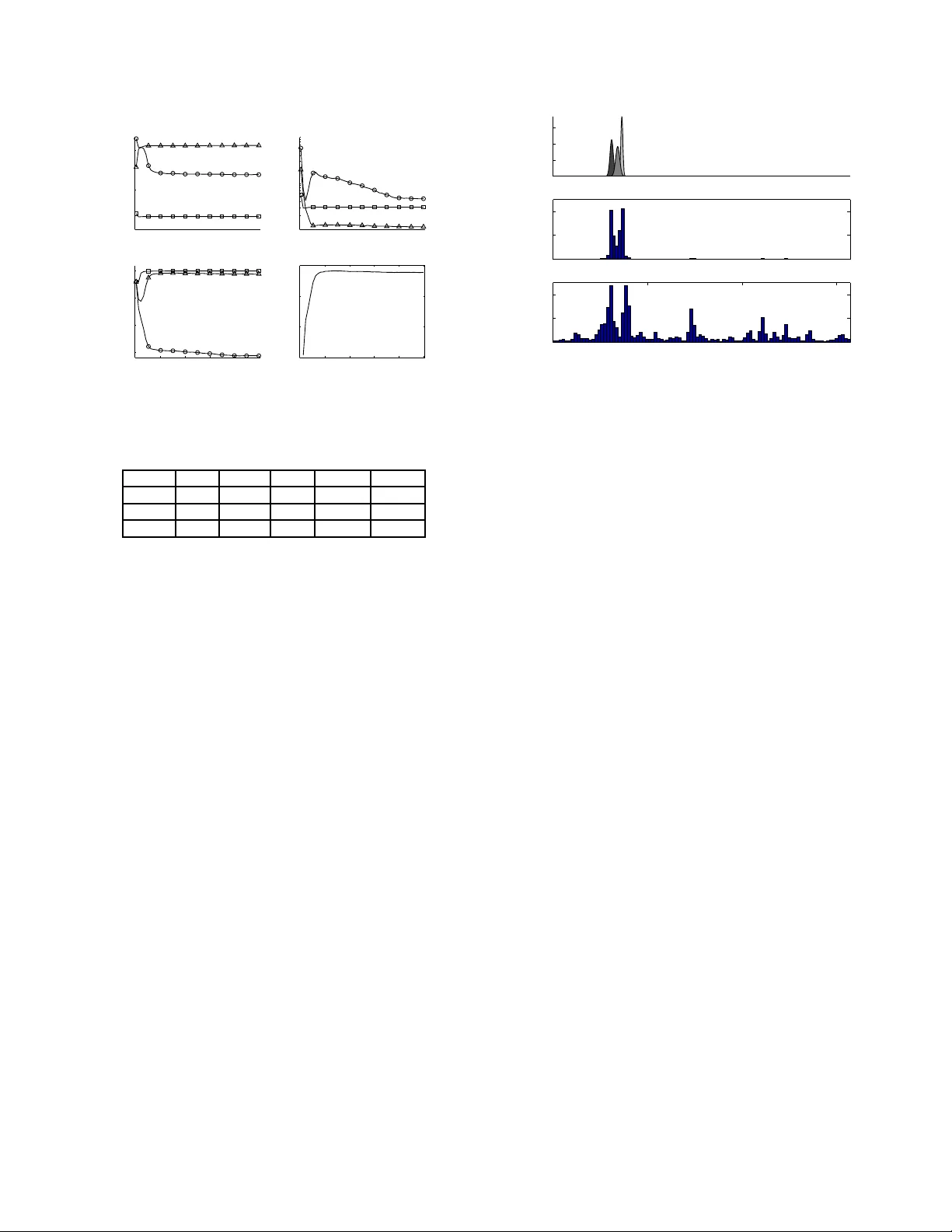
SUMMARIZING POSTERIOR DISTRIBUT IONS IN SIGNAL DECOMPOSITION PR OBLEMS WHEN THE NUMBER OF COMPONENTS IS UNKNO WN Alir eza Roodaki, J ulien Bect, and Gilles Fleury E3S—SUPELEC Systems Sciences Dept. of Signal Processing and Electronic Systems, SUPELEC, Gif-sur-Yv ette, F rance. Email: { alireza.roodaki, julien.bect, gilles.fleury } @supelec.fr ABSTRA CT This paper addresses the problem of summarizing the posterior distributions that typically arise, in a Bayesian framew ork, when dealing with signal decomposition problems wit h unknown number of components. Such posterior distributions are defined over union of subspaces of dif f ering dimensionality and can be sampled from using modern Monte Carlo t echniques, for instance the increasingly popular RJ-MCMC method . No generic approach is av ailable, how- e ver , to summarize the resulting variable-dimension al samples and extract fro m them component-spe cific parameters. W e propose a nov el approach to this problem, which consists in approximating the complex posterior of interest by a “simple”—bu t still v ariable-dimensional—parametric distribution. The distance between the two distrib utions is measured using the Kullback - Leibler diver gence, and a St ochastic E M-type al gorithm, driv en by the RJ-MCMC sa mpler , is proposed to estimate the parameters. The proposed algorithm is illustrated on the fundamental signal process- ing example of joint detection and estimation of sinusoids in white Gaussian noise. Index T erms — Bayesian inference; Posterior summarization; T r ans-dimensional MCMC; Label-switching; Stochastic EM. 1. INTRODUCTION No wadays, o wing to the advent of Markov C hain Monte Carlo (MCMC) sampling methods [1], Bayesian data analysis is consid- ered as a con ventional approach in machine learning, signal and image processing, and data mining problems—to name but a fe w . Ne vertheless, in many applications, practical challenges remain in the process of extracting, from the generated samples, quantities of interest to summarize the posterior distribution. Summarization consists, loosely speaking, in providing a fe w simple yet interpretable parameters and/or graphics to the end-user of a statistical method. For instance, in the case of a scalar parame- ter with a unimodal posterior distribution, measures of location and dispersion (e.g., the empirical mean and the standard deviation , or the median and the interquartile range) are t ypically provided in ad- dition to a graphical summary of the distr ibution (e.g., a histogram or a kerne l density estimate). In the case of multimodal distribu- tions summarization becomes more difficult but can be carried out using, for instance, the app roximation of the posterior by a Gaussian Mixture Model (GMMs) [2]. This paper addresses the problem of summarizing posterior dis- tributions in t he case of trans-dimensional problems, i.e. “the prob- lems in which the number of things that we don’ t kno w is one of the things that we don’t kno w” [3]. The problem of signal decomposi- tion when the number o f componen ts is u nkno wn is an imp ortant e x- ample of su ch p roblems. Let y = ( y 1 , y 2 , . . . , y N ) t be a v ector of N observ ations, where the superscript t stands for vecto r transposi- tion. In signal deco mposition pro blems, the model sp ace is a finite or countable set of models, M = {M k , k ∈ K} , where K ⊂ N is an index set. It is assumed here that, under M k , there are k compo nents with component-spec ific parameters θ k,j ∈ Θ ⊂ R d . W e denote by θ k = ( θ k, 1 , . . . , θ k,k ) ∈ Θ k the vector of component-spec ific parameters. In a Bayesian frame work, a joint posterior distribution is obtained through Bayes’ formula for the model index k and the vector of component-specific parameters, after assigning prior dis- tributions on them : f ( k, θ k ) ∝ p ( y | k , θ k ) p ( θ k | k ) p ( k ) , where ∝ indicates proportionality . This joint posterior distribution, defined over a union of subspaces of differing dimensionality , com- pletely describes t he information (and the associated uncertainty) provid ed by the data y about t he candidate models and the vecto r of unkno wn parameters. 1.1. Illustrative ex ample: sinusoid detection In this example, it is assumed that under M k , y can be written as a linear combination of k si nusoids observ ed in white Gaus- sian noise. The unknown component-specific parameters are θ k = { a k , ω k , φ k } , where a k , ω k and φ k are the vectors of amplitudes, radial frequencies and phases, respecti vely . W e use the hierarchical model, prior distributions, and Rev ersible Jump MCMC (RJ-MCMC) sampler [ 3] proposed in [4] f or this problem; the interested reader is thus referred to [3, 4] for more details. Figure 1 represents the posterior distributions of both the num- ber of components k and the sorted 1 radial frequencies ω k gi ven k obtained using the RJ-MCMC sampler . Each ro w is dedicated to one v alue of k , for 2 ≤ k ≤ 4 ; observe that, other models have negligi- ble posterior probabilities. In the expe riment, the observed signal of length N = 64 consists of t hree sinusoids with amplitudes a k = (20 , 6 . 32 , 20) t and radial frequencies ω k = (0 . 63 , 0 . 68 , 0 . 73) t . The SNR , k D k . a k k 2 N σ 2 is set to the moderate value of 7 d B , where D k is the design matrix and σ 2 is the noise v ariance. Roughly speaking, two approaches co-exist in the literature for such situations: Bayesian Model Selection (BMS) and Bayesian Model A v eraging (BMA). The BMS approach ranks models ac- cording to their posterior probabilities p ( k | y ) , selects one model, 1 Owing to t he in va riance of both the likelihoo d and the prior un der per- mutation of the components, component-spec ific marginal posteriors are all equal: this is t he “la bel-swit ching” phenomenon [5, 6 , 7]. Identifia bility con- straints (such as sorting) are the simplest way of deal ing with this issue. P S f r a g r e p l a c e m e n t s 59 . 5% 30 . 8% 7 . 8% k 5 9 . 5 3 0 . 8 7 . 8 ω k 0 . 5 0 . 75 1 2 3 4 Fig. 1 : Posteriors of k (left) and sorted radial frequencies, ω k , gi ven k (ri ght). The true number of compon ents is three. The vertical dashed lines in the right figure locate the true radial frequencies. and then summarizes the posterior under the (fi xed-d imensional) selected model. T his i s at t he price of l oosing valu able information provid ed by the other (discarded) models. For instance, in the ex- ample of Figure 1, all i nformation about t he small—and t herefore harder to detect—middle compo nent is lost by selecting the most a posteriori probable model M 2 . The BMA approach consists in reporting results that are av eraged over all possible models; it is, therefore, not appropriate for studying compone nt-specific parame- ters, the number of which changes in each model 2 . More information concerning these two approaches can be found in [3 ] and references therein. T o the best of our kno w ledge, no generic method i s currently av ailable, that would allow to sum- marize the information that i s so easily read on Figure 1 for this very simple exa mple: namely , that ther e seem to be three sinusoidal componen ts in the observed noisy signal, the middle one having a smaller pr obability of pr esence than the others . 1.2. Out line of the paper In this paper , we propose a novel approach to summarize the poste- rior distributions ov er variable-dimensiona l subspaces that typically arise in signal decomposition problems with an unkn o wn number of components. It consists in approximating the complex posterior distribution with a parametric model (of varying-dimen sionality), by minimization of t he Kullback -Leibler ( KL) di ver gence between the two distributions. A Stochastic EM (SEM)-type algorithm [8], driv en by the output of an RJ-MCMC sampler , is used to estimate the parameters of the approximate model. Our approach shares some simil arities wit h the relabeling algo- rithms proposed in [6, 7] to solv e th e “label switching” prob lem, and also with the EM algorithm used in [9 ] in the context of adaptiv e MCMC algorithms (both in a fixed -dimensional setting). The main contribution of this paper is the introduction of an original variable- dimensional parametric model, which allo w s to tackle directly the difficu lt problem of approximating a distri bution defined ov er a union of subspaces of differing dimensionality—and thus provides a fi rst solution to the “trans-dimensional label-switching” problem, 2 See, howe ver , the intensi ty plot provided in Section 3 (middle plot on Figure 4) as a n exampl e of a BMA summary relate d to a componen t-specific paramete r . so to speak. The paper is organ ized as follows. Section 2 introduces the pro- posed model and stochastic algorithm. Section 3 il lustrates the ap- proach using the sinusoid detection e xample already discussed in the introduction. F inally , Section 4 conclud es the paper and gi ves direc- tions for future work. 2. PROPOSED ALGORITHM Let F denote the target posterior distribution, defined on the v ariable-dimensional space X = S k max k =0 { k } × Θ k . W e assume that F admits a probability density f unction (pdf) f , wit h respect to the k d -dimensional Lebesgue measure on each { k } × Θ k , k ∈ K . T o keep things simple, we also assume that Θ = R d . Our objectiv e i s to approximate the exa ct posterior density f using a “simple” parametric model q η , where η is the vector of parameters defining the model. The pdf q η will also be de- fined on the variable-dimensio nal space X (i.e., it is not a fi xed- dimensional approx imation as in the BMS approa ch). W e assume that a Monte Carlo sampling method is av ailable, e.g. a RJ-MCMC sampler [3], to gen erate M samples fro m f , which we deno te by x ( i ) =  k ( i ) , θ ( i ) k ( i )  , for i = 1 , . . . , M . 2.1. V ariable-dimensional parametric model Let us describe the proposed parametric model from a generati ve point of vie w . As in a traditi onal GMM, we assume t hat there is a certain numbe r L of “Gaussian components” in the ( approximate) posterior , each generating a d -variate Gaussian v ector with mean µ l and co v ariance matrix Σ l , 1 ≤ l ≤ L . An X -va lued random variable x = ( k , θ k ) , with 0 ≤ k ≤ L , is generated as f ollo ws. F irst, each of the L compone nts can be ei- ther present or absent according to a binary indicator v ari able ξ l ∈ { 0 , 1 } . These Bernoulli variables are assumed to be independent, and we denote by π l ∈ (0; 1] the “probability of presence” of the l th Gaussian component. Second, giv en the indicator va riables, k = P L l =1 ξ l Gaussian vectors are generated by the Gaussian compo- nents that are present ( ξ l = 1 ) and randomly arranged in a vector θ k = ( θ k, 1 , . . . , θ k,k ) . W e denote by q η the pdf of the random v ari able x that is thus generated, with η l = ( µ l , Σ l , π l ) the vector of p arameters of the l th Gaussian compon ent, 1 ≤ l ≤ L , and η = ( η 1 , . . . , η L ) . Remark. In contrast with GMMs, where only one component is present at a t ime (i.e., k = 1 in our notations), there is no constraint here on the sum of the probabilities of presence. 2.2. Estimating the model parameters One way to fit the parametric distrib ution q η ( x ) to the p oste- rior f ( x ) is to minimize the KL di vergence of f from q η , denoted by D K L ( f ( x ) k q η ( x )) . Thus, we define the criterion to be minimized as J ( η ) , D K L ( f ( x ) k q η ( x )) = Z X f ( x ) log f ( x ) q η ( x ) d x . Using samples generated by the RJ-MCMC sampler , this crit erion can be approx imated as J ( η ) ≃ ˆ J ( η ) = − 1 M M X i =1 log  q η ( x ( i ) )  + C . At the r th iteration, S-step draw allocation vectors z ( i,r ) ∼ p  · | x ( i ) , ˆ η ( r − 1)  , for i = 1 , . . . , M . M-step estimate ˆ η ( r ) such that ˆ η ( r ) = argmax η M X i =1 log p  x ( i ) , z ( i,r ) | η  . Fig. 2 : SEM algorithm. where C is a constant that does not depend on η . One should note that minimizing ˆ J ( η ) amounts t o estimating η such t hat ˆ η = argmax η M X i =1 log  q η ( x ( i ) )  . (1) No w , we assume that each element of the i th observ ed sam- ple x ( i ) j , for j = 1 , . . . , k i , has arisen from one of the L Gaussian componen ts contained in q η . At this point, i t is natural to introduce allocation v ectors z ( i ) correspondin g to the i th observ ed sample x ( i ) , for i = 1 , . . . , M , as latent va riables. The element z ( i ) j = l indi- cates that x ( i ) j is allocated to the l th Gaussian component. Hence, gi ven the allocation ve ctor z ( i ) and the parameters of th e model η , the conditional distribution of the observed samples, i.e., the model’ s likelihood, is p ( x ( i ) | z ( i ) , η ) = k ( i ) Y j =1 N ( x ( i ) j | µ z ( i ) j , Σ z ( i ) j ) . It turns out that the E M-type algorithms, which have been used in si milar works [6, 7, 9], are not appropriate for solving this prob- lem, as computing the expectation in the E- step is intricate. More explicitly , in our problem the computational burde n of the summa- tion in the E-step over the set of all possible allocation vectors z increases very rapidly wit h k . In fact, e ven for moderate values of k , say , k = 10 , t he summation is far too expe nsiv e to compute as it in volv es k ! ≈ 3 . 6 10 6 terms. In this paper , we propose t o use SEM [8], a v ariation of the EM algorithm in which the E-step is substituted with st ochastic simulation of the latent v ariables fr om their conditiona l posterior distributions gi ven the previous estimates of the unkn o wn parameters. In other words, for i = 1 , . . . , M , t he allocation vectors z ( i ) are drawn from p ( · | x ( i ) , ˆ η ( r ) ) . This step is called the Stochastic (S)-step. Then, these r andom samples are used to construct the so-called pseud o-completed l ikelihood which reads p  x ( i ) , z ( i ) | η  = k ( i ) Y j =1 N  x ( i ) j | µ z ( i ) j , Σ z ( i ) j  × 1 Z ( z ( i ) ) k ( i ) ! L Y l =1 π ξ ( i ) l l (1 − π l ) (1 − ξ ( i ) l ) , (2) where Z is the set of all allocation vectors and ξ ( i ) l = 1 if and only if there is a j ∈ { 1 , . . . , k ( i ) } such that z ( i ) j = l . The proposed SEM-type algorithm for our problem is described in Figure 2. Direct sa mpling from p ( · | x ( i ) , ˆ η ( r ) ) , as required by the S-step, is unfortunately not feasible. Instead, since p ( z ( i ) | x ( i ) , ˆ η ( r ) ) ∝ p ( x ( i ) , z ( i ) | ˆ η ( r ) ) can be computed up to a normalizing constant, we de vised an Independe nt Metropolis-Hasting (I-MH) algorithm to construct a Marko v chain with p ( z ( i ) | x ( i ) , ˆ η ( r ) ) as i ts stationary distribution. 2.3. Robustified algorithm Preliminary experiments with the model and method described in the pre vious sections prov ed to be disappointing. T o understand why , it must be remembered t hat the pdf q η we are looking for is only an appr oximation (hope fully a good o ne) of the true po sterior f . For in- stance, for high v alues of k , the posterior typically in volv es a diffuse part which can not properly represented by the parametric model (this can be seen quite clearly for k = 4 on Figure 1). Therefore, for any η , some samples generated by t he RJ-MCMC sampler are outliers with respect t o q η (i.e., the true posterior can be considered as a contaminated ve rsion o f q η ) w hich causes pro blems when using a maximum likelihoo d-type estimate such as (1). These rob ustness issues were solv ed, in this paper , using two modifications of the algorithm (only i n the one-dimensional case up to now). F irst, robust estimates [10] of the means and v ariances of a Gaussian distribution, based on the median and the interquartile range, are used instead of the empirical means and variances in the M-step. Second, a Poisson process component (with uniform inten- sity) i s added to the model, i n order to account for the diffuse part of the posterior and allow for a number L of Gaussian componen ts which is smaller than the maximum observ ed k ( i ) . Remark. S imilar rob ustness concerns are widespread in t he cluster- ing literature; see, e.g., [11] and the references therein. 3. RESUL TS In this section, we will in vestigate the capability of the proposed algorithm for summarizing variable-dimensiona l posterior distribu- tions. W e emphasize again that the output of the trans-dimensional Monte Carlo sampler , e.g. RJ-MCMC in this paper , is considered as the observed data for our algorithm. Regarding t he fact that in this paper we pro vide results for the sinusoids’ radial frequencies, the proposed parametric model consists of uni v ariate Gaussian compo- nents. In other words, the space of component-specific parameters Θ = (0; π ) ⊂ R . But we belie ve that our algorithm is not limited to the problems with one-dimensional componen t-specific parameters. Therefore, in this section, it is assumed that each Gaussian compo- nent has a mean µ , a variance s 2 , and a probability of presence π to be estimated. Before launching t he algorithm, first, we need to initiali ze the parametric model. It is natural to deduce the number L of Gaussian componen ts from the posterior distribution of k . Here, we set it to the 90 th percentile to ke ep all the probable models in the play . T o initialize the Gaussian components’ parameters, i.e. µ and s 2 , we used the robust estimates of the posterior of the sorted radial frequencies gi ven k = L . W e ran the “rob ustified” stochastic algorithm introdu ced in Sec- tion 2 on the specific example shown in Figure 1, for 50 iterations, with L = 3 G aussian co mponents (the posterior probability of { k ≤ 3 } i s approximately 90.3%). Figure 3 illustrates the ev olution of model parameters η together with the crit erion J . T wo substan- tial facts can be deduced from this figure; first, the increasing be- havior of the criterion J , which is almost constant after t he 10 th iteration. Second, the con vergen ce of the parameters of parametric model, esp. means µ and prob abilities of presenc e π , though usin g a nai ve initiali zation procedure. Indeed after the 40 th iteration there is no significant mov e i n the parameter estimates. T able 1 presents the P S f r a g r e p l a c e m e n t s µ s 2 π SEM iteration J SEM iteration 10 20 30 40 50 10 20 30 40 50 0 5 1 0 1 5 2 0 2 5 3 0 3 5 4 0 4 5 5 0 0 5 1 0 1 5 2 0 2 5 3 0 3 5 4 0 4 5 5 0 1 2 3 0 . 25 0 . 5 0 . 75 1 10 − 4 10 − 3 10 − 2 0 . 6 0 . 66 0 . 72 Fig. 3 : Performance of the proposed summarizing algorithm on the sinusoid detection example. There are three Gaussian compon ents in the model. Comp µ s π µ BM S s BM S 1 0 . 62 0 . 01 7 1 0 . 62 0 . 016 2 0 . 68 0 . 02 1 0 . 22 — — 3 0 . 73 0 . 01 1 0 . 97 0 . 73 0 . 012 T able 1 : Summaries of the variable-dimen sional posterior distribu- tion sho wn i n Figure 1; The proposed approach vs. BMS. summaries provided by the proposed method along with the ones obtained using the B MS approach . Contrary to BMS, the method that we proposed has enabled us to benefit from the information of all probable models to giv e summaries about the middle harder to detect component. Turnin g to the r esults of our approach, it can be seen that the estimated means are compatible wit h the true radial frequencies. Furthermore, t he estimated probabilities of presence are consistent with uncertainty of them in the variab le-dimensional posterior sho wn in F igure 1. Note the small estimated standard de- viations which indicate our robu stifying strategies ha ve been useful. The pdf ’ s of the estimated Gaussian compo nents are sho wn i n Figure 4 (top). Comparing with t he posterior of sorted radial fre- quencies sho wn in Figure 1, it can be inferred that the proposed al- gorithm has managed to remo ve the label-switching pheno menon i n a variable-dimension al problem. Furthe rmore, the intensity plot of the all ocated samples to the point process component is depicted in Figure 4 (bottom). This presents the outliers in the observed samples which cannot be be described by the Gaussian compon ents. Note that withou t the po int process comp onent these outliers w ould be a l- located to the Gaussian components which can, consequently , yield in a significant deterioration of parameter estimates. 4. CONCLUSION In this paper , we ha ve proposed a novel algorithm to summarize pos- terior distr ibutions defined ov er union of subspaces of dif f ering di- mensionality . For this purpose, a variable-dimension al parametric model has been designed to approximate the posterior of interest. The parameters of the approximate model hav e been estimated by means of a SEM-type algo rithm, using samples from the posterior f generated by an RJ-MCMC algorithm. Modifications of our initial P S f r a g r e p l a c e m e n t s pdf intensity intensity ω k 0 1 2 3 0 0 . 5 1 1 . 5 2 2 . 5 3 0 0 . 5 1 1 . 5 2 2 . 5 3 0 1 2 0 10 20 0 10 20 30 Fig. 4 : The pdf of fit ted Gaussian components (top), the histogram intensity of all radial frequencies samples (middle), and the his- togram intensity of the allocated samples to t he Poisson point pro- cess compone nt (bottom). SEM-type algorithm have been proposed, in order to cope with the lack of robustness of maximum likelihood-type estimates. The rel- e v ance of the proposed algorithm, both for summarizing and for re- labeling v ari able-dimensional posterior distributions, h as been illus- trated on the problem of detecting and estimating sinusoids in Gaus- sian white noise. W e believ e that this algorithm can be used in the vast domain of signal decomposition and mixture model analysis to enhance in- ference in t rans-dimensional problems. For t his purpose, generaliz- ing the proposed algorithm t o the m ultiv ariate case and an alyzing its con verge nce properties is considered as future work. Another impor- tant point would be to use a more reliable initialization proce dure. Refer ences [1] C.P . Robert a nd G. Casella, Monte Carlo Statistical Methods (se cond edition) , Springer V erlag, 2004. [2] M. W est, “Approximating posterior distrib utions by mixture, ” J. Roy . Stat. Soc. B Met. , vol. 55, no. 2, pp. 409–422, 1993. [3] P . J. Green, “R ever sible jump MCMC computation and B ayesian model determi- nation, ” Biometrika , vol. 82, no. 4, pp. 711–732, 1995. [4] C. Andrieu and A. Douce t, “Joint Bayes ian model s election and estimation of noisy s inusoids via reversible jump MCMC,” IEEE Trans. Signal Process. , vol. 47, no. 10, pp. 2667–2676, 1999. [5] S. Richardson and P . J . Green, “On Baye sian analysis of mixtures with an un- known number of components, ” J. Roy. Stat. Soc. B Met. , vol. 59, no. 4, pp. 731–792, 1997. [6] M. Stephens, “Dealing with label switching i n mixture models, ” J. Roy. Stat. Soc. B Met. , pp. 795–809, 2000. [7] M. Sperrin, T . J aki, a nd E. Wit, “Probabilistic relabelling s trategies for the label switching problem in bayesian mixture models, ” Stat. and Comput. , vol. 20, pp. 357–366, 2010. [8] G. Celeux and J. Diebolt, “The SEM algorithm : a probabilistic teacher algorithm deriv ed from t he EM algorithm for the mixture problem, ” C omp. Statis. Quaterly , vol. 2, pp. 73–82, 1985. [9] Y . Bai, R. V . Craiu, and A. F . Di Narzo, “Divide and conquer: a mixture-based approach to regional adaptation f or MCMC, ” J. Comput. Gra ph. Stat. , , no. 0, pp. 1–17, 2011. [10] P . J. Huber and E . M. Ronchetti, R obust statistics (2nd Edition) , Wil ey ., 2009. [11] R.N. Dav ´ e a nd R. Krishnapuram, “Robust clustering methods: a unified view , ” IEEE T rans. Fuzzy Sys. , vol. 5, no. 2, pp. 270–293, 1997.