Optimization with Sparsity-Inducing Penalties

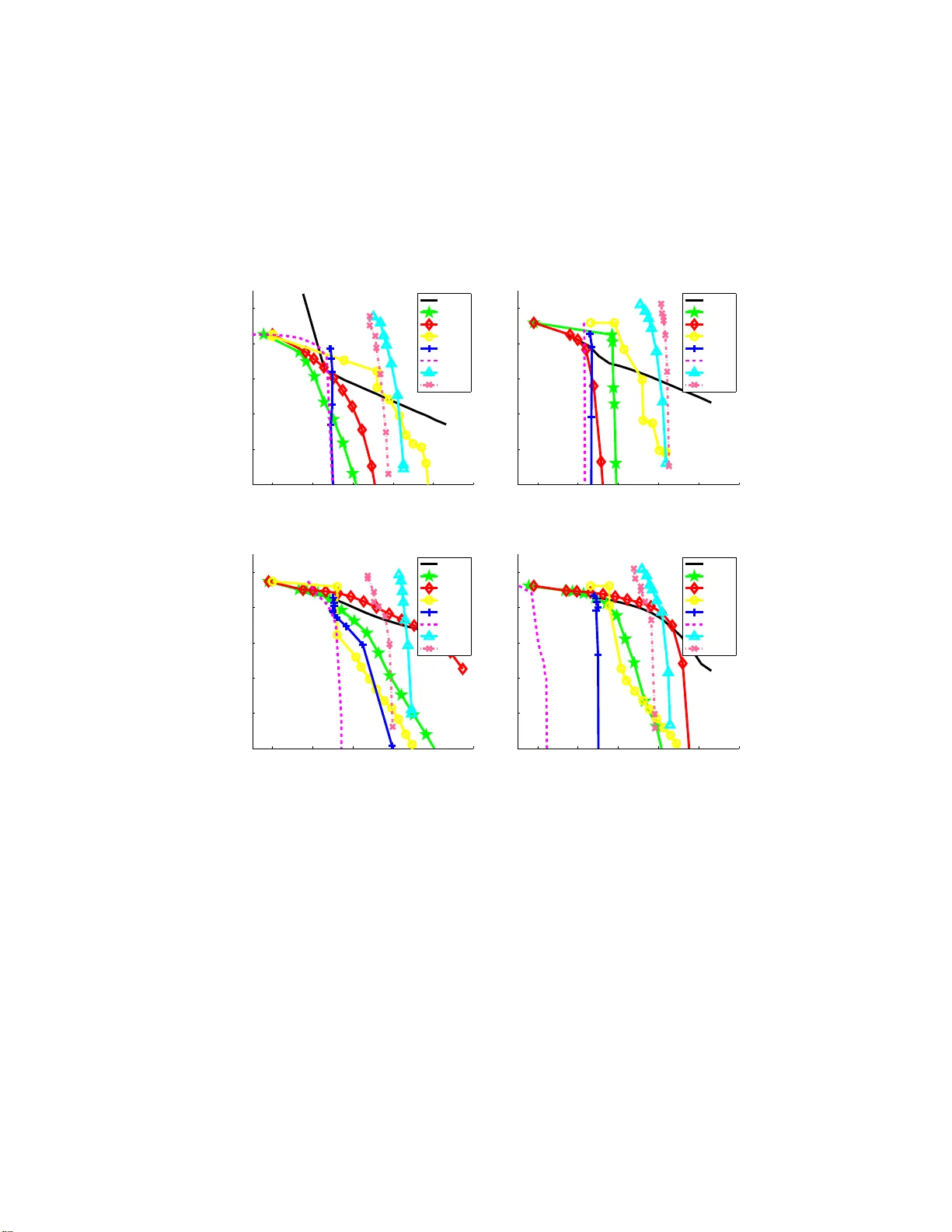
Optimization with Spa rsit y-Inducin g P enalties F rancis Bac h 1 , Ro d olphe Jenatton 2 , Julien Mairal 3 and Guillaume Ob ozinski 4 1 INRIA - SIERRA Pr oje ct-T e a m, L ab or atoir e d’Informa tique de l’Ec ole Normale Sup´ erieur e, 23 , avenue d’Italie, Paris, 7501 3, F r a nc e, fr an- cis.b ach @inria.fr 2 INRIA - SIERRA Pr oje ct-T e am, r o dolphe.j enatt on@inria.fr 3 Dep artmen t of Statistics, Un iversity of California , Berkeley, CA 94720- 1776, USA, julien@stat.b erkeley.e du 4 INRIA - SIERRA Pr oje ct-T e am, guil laume.ob ozinski@inria.fr Abstract Sparse estimation metho ds are aimed at usin g or obtaining parsimo- nious represent ations of data or mo dels. Th ey were ﬁrst dedicated to linear v ariable selection b ut n um er ou s extensions hav e n o w emerged suc h as s tructured sparsity or k ernel s electio n . It turn s out that many of the related estimat ion problems can b e cast as conv ex optimiza- tion problems b y regularizing the empirical risk with appropriate non- smo oth n orm s. The goal of this pap er is to presen t from a general p er- sp ectiv e o ptimization tools and te chniques dedicated to s uc h sparsit y- inducing p enalties. W e cov er pro ximal metho ds, blo c k-co ord inate de- scen t, reweig hted ℓ 2 -p enalized tec hn iqu es, wo r k in g-set and homotop y metho ds, as w ell as n on-con v ex formulations and extensions, and pro- vide an extensive set of exp erimen ts to compare v arious algorithms from a computational p oin t of view. Contents 1 In tro duction 1 1.1 Notatio n 5 1.2 Loss F unctions 6 1.3 Sparsit y-In d ucing Norms 7 1.4 Optimization T o ols 15 1.5 Multiple Kernel Learning 31 2 Generic Metho ds 38 3 Pro ximal Metho ds 41 3.1 Principle of Proxima l Metho d s 41 3.2 Algorithms 43 3.3 Computing the Pro ximal Op erator 44 3.4 Pro ximal Metho ds for Structur ed MKL 49 4 (Blo c k) Co ordinate Descen t Algorithms 54 i ii Con tents 4.1 Co ordinate Descen t for ℓ 1 -Regularizati on 54 4.2 Block-Coordin ate Descen t for ℓ 1 /ℓ q -Regularizati on 56 4.3 Block-coordinate descent f or MKL 58 5 Rew eigh te d- ℓ 2 Algorithms 59 5.1 V ariational formulatio n s for group ed ℓ 1 -norms 59 5.2 Quadratic V ariational F orm ulation for General Norms 61 6 W orking-Set and Homotop y Met ho ds 65 6.1 W orking-Set T ec hniques 65 6.2 Homotop y Metho d s 67 7 Sparsit y and N onconv ex Opt imization 72 7.1 Greedy Algorithms 72 7.2 Rew eigh ted- ℓ 1 Algorithms with DC-Programming 75 7.3 Sparse Matrix F actorization and Dictionary Learning 77 7.4 Ba y esian Metho ds 79 8 Quan tit ativ e Ev aluation 82 8.1 Sp eed Benc hmarks for Lasso 83 8.2 Group-Sparsity for Multi-task Learning 87 8.3 Structured Sparsity 88 8.4 General Commen ts 94 9 Extensions 96 10 Conclusions 98 Ac kno wledgements 101 References 102 1 Intro duction The principle of pars im ony is central to man y areas of science: the sim- plest explanation of a giv en phen omenon should b e preferred o v er m ore complicated ones. In the con text of m ac hine learning, it tak es the form of v ariable or f eature selection, and it is commonly used in t wo situa- tions. First, to mak e the mo del or the prediction more in terpretable or computationally c heap er to use, i.e., eve n if the un derlying problem is not sparse, one lo oks for the b est sparse approxima tion. S econd, spar- sit y can also b e used give n pr ior kn o wledge that the mo del should b e sparse. F or v ariable selection in linear mo d els, parsim ony m a y b e directly ac hiev ed by p enalization of the empirical risk or the log-lik eliho o d by the cardinalit y of the supp ort 1 of the w eigh t vect or. How ever, this leads to h ard com binatorial pr oblems (see, e.g., [97, 137]). A traditional con- v ex app ro ximation of th e problem is to replace th e cardinalit y of the supp ort by the ℓ 1 -norm. Estimators may then b e obtained as solutions of con ve x pr ograms. Casting spars e estimat ion as con vex optimization problems has 1 W e call the set of non-zeros en tries of a v ector the s upport. 1 2 Introduction t w o main b eneﬁts: First, it leads to eﬃcien t estimat ion algorithms— and this pap er fo cus es pr imarily on these. Second, it allo ws a fruit- ful theoretica l analysis answering fundamen tal questions related to es- timation consistency , p r ediction eﬃciency [19, 100] or mo d el consis- tency [145, 158]. In particular, when the spars e mo del is assumed to b e well -sp eciﬁed, regularization by the ℓ 1 -norm is ad ap ted to h igh- dimensional problems, where the n umb er of v ariables to learn from ma y b e exp onent ial in the n u mb er of observ ations. Reducing parsimon y to ﬁnding the mo del of lo west cardinalit y turns out to b e limiting, and structur e d p arsimony [15, 65, 63, 67] has emerged as a natural extension, w ith applicat ions to computer vision [32, 63, 71], text pro cessing [69], bioinformatics [65, 74] or au- dio pro cessing [81]. S tructured sparsit y ma y b e ac hiev ed by p enalizing other fu nctions than the cardin alit y of the su pp ort or r egularizing by other norms than the ℓ 1 -norm. In this pap er, w e fo cus primarily on norms which can b e written as linear combinatio ns of n orm s on subsets of v ariables, but w e also consider traditional extensions suc h as mul- tiple ke rn el learning and sp ectral norm s on matrices (see Sections 1.3 and 1.5). One m ain ob jectiv e of this pap er is to presen t metho ds whic h are adapted to most sparsit y-inducing norms with loss functions p o- ten tially b eyo nd least-squares. Finally , similar to ols are used in other communities suc h as signal pro cessing. While the ob jectiv es and the problem set-ups are diﬀerent , the resulting conv ex optimizati on problems are often similar, and most of the tec hniqu es review ed in this pap er also app ly to sparse estimation problems in signal p ro cessing. Moreo ve r, w e consider in Section 7 non- con v ex formulat ions and extensions. This pap er aims at p ro viding a general o v erview of the main opti- mization tec hn iqu es that hav e emerged as most relev ant and eﬃcien t for metho ds of v ariable selection based on sp ars it y-inducing n orms. W e surve y and compare sev eral algorithmic app r oac h es as th ey apply to the ℓ 1 -norm, group norms, but also to n orms inducing structured spar- sit y and to general m ultiple k ernel learning problems. W e complemen t these by a pr esen tation of s ome greedy and n on-con v ex metho ds. Ou r present ation is essen tially b ased on existing literature, but the pro cess of constructing a general framew ork leads naturally to new results, 3 connections and p oints of view. This monograph is organized as follo ws: Sections 1.1 and 1.2 intro d uce resp ectiv ely the notati ons us ed throughout the manuscript and th e optimization problem (1.1) wh ic h is cen tral to th e learning framework that we will consider. Section 1.3 giv es an o verview of common sp arsit y and structured sparsit y-indu cing norms, w ith some of their prop erties and examples of structures whic h th ey can enco de. Section 1.4 p ro vides an essen tially self-con tained presen tation of concepts and to ols from conv ex analysis that will b e needed in the rest of the m anuscript, and whic h are relev ant to understand algorithms for solving th e main optimization problem (1.1). S p eciﬁcally , since sparsit y inducing n orms are non-diﬀerentia ble con vex functions 2 , we in tro du ce relev an t element s of subgradien t theory and F enchel dualit y—which are particularly we ll suited to form ulate the optimalit y conditions as- so ciated to learning problems regularized with these norms. W e also in tro d u ce a general qu adratic v ariational formulat ion f or a certain class of norm s in S ection 1.4.2; the part on sub quadratic norms is essen tially relev an t in view of sections on stru ctured m ultiple kernel learning and can safely b e skip p ed in a ﬁrst reading. Section 1.5 introd uces multiple kernel le arning (MKL) and s h o ws that it can b e interpreted as an extension of plain sp arsit y to repro- ducing k ernel Hilb ert spaces (RKHS ), b ut formulated in the d ual. Th is connection is fu rther exploited in Section 1.5.2, where its is sh own ho w stru ctured counte rp arts of MKL can b e asso ciated with struc- tured sparsit y-inducing norms. These sections rely on Section 1.4.2. All sections on MKL can b e skipp ed in a ﬁrst reading. In Section 2, we discuss classical app roac hes to solving th e opti- mization problem arising from simple sparsit y-inducing norms, suc h as in terior p oin t metho d s and subgradient descen t, and p oin t at their shortcomings in the con text of mac hine learning. 2 Throughout this paper , we refer to sparsity-inducing norms suc h as the ℓ 1 -norm as non- smo oth norms; note that all nor m s are non-diﬀerentiable at zero, but some norms hav e more non-diﬀerentiabilit y p oint s (see more details in Section 1.3). 4 Introduction Section 3 is dev oted to a simple pr esen tation of pr o ximal metho ds. After t wo short sections in tro du cing th e main concepts and algorithms, the longer S ection 3.3 fo cusses on the pr oximal op er ator and present s algorithms to compute it for a v ariet y of norms. S ection 3.4 shows ho w pro ximal metho d s for structured n orms extend naturally to the RKHS/MKL setting. Section 4 presents blo c k co ordin ate descen t algorithms, which pro- vide an eﬃcient alt ern ativ e to pro ximal metho d for sep ar able norms lik e the ℓ 1 - and ℓ 1 /ℓ 2 -norms, and can b e applied to MKL. This section uses the concept of proximal op erator int ro duced in Section 3. Section 5 presents reweig hted- ℓ 2 algorithms that are b ased on th e quadratic v ariational form u lations in tro d uced in Sectio n 1.4.2. These algorithms are particularly relev ant for the least-squares loss, for which they take the form of iterat ive rew eigh ted least-squares algorithms (IRLS). S ection 5.2 pr esents a generally applicable quadratic v aria- tional form u lation for general n orms th at extends the v ariational for- m ulation of S ection 1.4.2. Section 6 co v ers algorithmic schemes that tak e adv an tage computa- tionally of the spars it y of the solution b y extending the supp ort of the solution grad u ally . These s chemes are particularly relev an t to construct appro ximate or exact regularizat ion p aths o f solutions for a range of v al- ues of the regularization parameter. S p eciﬁcally , Section 6.1 pr esen ts w orking-set tec hniqu es, whic h are meta-algorithms th at can b e used with th e optimization sc hemes pr esen ted in all the p revious c hapters. Section 6.2 fo cuses on the homotop y algorithm, whic h can eﬃcien tly construct the en tire regularization path of th e Lasso. Section 7 presents nonconv ex as we ll as Ba y esian approac h es that pro vide alternativ es to, or extensions of the conv ex metho ds that were present ed in the p revious sections. More precisely , Section 7.1 presen ts so-calle d greedy algo rithm s , that aim at solving the cardinalit y con- strained p roblem and in clud e matc hin g pur suit, orthogonal matching pursu it and f orw ard s electio n ; S ection 7.2 presents contin u ous opti- mization pr oblems, in whic h the p en alty is chosen to b e closer to the so-calle d ℓ 0 -p enalt y (i.e. , a p enalization of the cardinalit y of the mo del regardless of the amplitude of the coeﬃcient s) at the exp en se of losing 1.1. Notation 5 con v exit y , and corresp ondin g optimiza tion schemes. Section 7.3 dis- cusses the application of sparse norms regularization to the problem of m atrix factoriza tion, whic h is intrinsicall y non conv ex, bu t for whic h the algorithms pr esen ted in the rest of this monograph are relev an t. Fi- nally , w e discuss brieﬂy in Section 7.4 Bay esian app roac hes to sp arsit y and the relations to sp ars it y-inducing norms. Section 8 pr esen ts exp eriments comparin g th e p erformance of the algorithms presente d in S ections 2, 3, 4, 5, in terms of sp eed of con- v ergence of the algorithms. Precisely , Section 8.1 is dev oted to th e ℓ 1 - regularization case, and S ection 8.2 and 8.3 are resp ectiv ely co vering the ℓ 1 /ℓ p -norms with disj oin t groups and to more general structured cases. W e discuss br ieﬂy metho ds and cases wh ic h were not co v ered in the rest of the monograph in S ection 9 and w e conclude in Section 10. Some of the material f rom this pap er is take n from an earlier b o ok c hapter [12] and the dissertations of Ro dolph e Jenatton [66] and Julien Mairal [86]. 1.1 Notation V ectors are denoted b y b old low er case letters and matrices b y up- p er case ones. W e deﬁn e for q ≥ 1 th e ℓ q -norm of a vecto r x in R n as k x k q := ( P n i =1 | x i | q ) 1 /q , where x i denotes the i -th co ordinate of x , and k x k ∞ := max i =1 ,...,n | x i | = lim q →∞ k x k q . W e also deﬁne the ℓ 0 -p enalt y as the n u mb er of nonzero elemen ts in a v ector: 3 k x k 0 := # { i s.t. x i 6 = 0 } = lim q → 0 + ( P n i =1 | x i | q ). W e consider the F rob enius norm of a m a- trix X in R m × n : k X k F := ( P m i =1 P n j =1 X 2 ij ) 1 / 2 , where X ij denotes the en try of X at ro w i and column j . F or an integer n > 0, and for any subset J ⊆ { 1 , . . . , n } , w e d enote by x J the v ector of size | J | conta inin g the entries of a v ector x in R n indexed b y J , and by X J the matrix in R m ×| J | con taining the | J | columns of a matrix X in R m × n indexed b y J . 3 Note that it would be more proper to write k x k 0 0 instead of k x k 0 to be consisten t with the traditional notation k x k q . How eve r , for the sake of simpl icity , we will ke ep this notation unc hanged in the rest of the pap er. 6 Introduction 1.2 Loss Functions W e consider in th is p ap er con v ex optimization p roblems of the form min w ∈ R p f ( w ) + λ Ω( w ) , (1.1) where f : R p → R is a conv ex d iﬀeren tiable fu n ction and Ω : R p → R is a sparsit y-ind ucing—t ypically n onsmo oth and non-Euclidean—norm. In sup er v ised learning, w e pr edict outputs y in Y from obser- v ations x in X ; these observ ations are usually represented by p - dimensional v ectors w ith X = R p . In this sup ervised setting, f generally corresp onds to th e empirical risk of a loss f unction ℓ : Y × R → R + . More precisely , giv en n pairs of data p oin ts { ( x ( i ) , y ( i ) ) ∈ R p × Y ; i = 1 , . . . , n } , w e h a v e for linear mo d els 4 f ( w ) := 1 n P n i =1 ℓ ( y ( i ) , w ⊤ x ( i ) ). Typica l examples of diﬀeren tiable loss functions are the square loss for least squares regression, i.e., ℓ ( y , ˆ y ) = 1 2 ( y − ˆ y ) 2 with y in R , and the logistic loss ℓ ( y , ˆ y ) = log (1 + e − y ˆ y ) for log istic regression, with y in {− 1 , 1 } . Clearly , several loss fun ctions of in terest are non-diﬀerentia ble, suc h as the hinge loss ℓ ( y , ˆ y ) = (1 − y ˆ y ) + or the absolute d eviation loss ℓ ( y , ˆ y ) = | y − ˆ y | , for wh ic h most of the approac h es w e present in this monograph wo uld not b e app licable or requir e app ropriate mo d iﬁ ca- tions. Giv en the tutorial c haracter of this monograph, we restrict our- selv es to smo oth fu n ctions f , whic h we consider is a reasonably broad setting, and w e refer the inte rested reader to appropriate references in Section 9. W e r efer the readers to [127] for a more complete d escrip tion of loss functions. P enalty or constrain t ? Giv en our conv ex data-ﬁtting term f ( w ), w e consider in this pap er addin g a con vex p enalt y λ Ω( w ). Within such a con v ex optimiza tion framew ork, this is essential ly equiv alent to add ing a constrain t of the form Ω( w ) ≤ µ . More precisely , und er w eak as- sumptions on f and Ω (on top of con v exit y), from Lagrange multiplier theory (see [20], Section 4.3) w is a solution of the constrained p roblem for a certain µ > 0 if and only if it is a solution of the p enalized prob- lem for a certain λ ≥ 0. T h us, the t wo r egularization paths, i.e., the 4 In Section 1.5, we consider extensions to non-linear predictors through multiple kernel learning. 1.3. Sparsit y-I nducing Norms 7 set of solutions when λ and µ v ary , are equiv alen t. Ho wev er, there is no d irect mapping b et wee n corresp onding v alues of λ and µ . Moreo ver, in a mac hine learning context , w h ere th e parameters λ and µ hav e to b e selected, for example through cross-v alidation, the p en alized for- m ulation tends to b e empirically easier to tun e, as th e p erformance is usually quite r obust to sm all c h an ges in λ , while it is not robust to small c hanges in µ . Finally , w e could also replace the p enalization with a norm by a p enalizatio n with the squ ared n orm. Indeed, follo wing the same reasoning as for the non-squared n orm, a p enalt y of the form λ Ω( w ) 2 is “equiv alen t” to a constraint of the form Ω( w ) 2 6 µ , whic h itself is equiv alen t to Ω ( w ) 6 µ 1 / 2 , and thus to a p enalt y of th e form λ ′ Ω( w ) 2 , for λ ′ 6 = λ . T h us , using a squared norm, as is often done in the con text of multiple kernel learning (see Section 1.5), do es not c han ge the regularization pr op erties of the formula tion. 1.3 Spa rsit y-Induc ing Norms In this section, we presen t v arious norms as well as their m ain sp arsit y- inducing eﬀects. These eﬀects ma y b e illustrated geometrica lly throu gh the singularities of the corresp onding unit balls (see Figure 1.4). Sparsit y through the ℓ 1 -norm. When one knows a priori that the solutions w ⋆ of problem (1.1) sh ould ha ve a few non -zero co eﬃcient s, Ω is often chose n to b e the ℓ 1 -norm, i.e., Ω( w ) = P p j =1 | w j | . Th is leads for in stance to the Lasso [134] or b asis pu rsuit [37] with the square loss and to ℓ 1 -regularized logistic regression (see, for instance, [76, 128]) with the logistic loss. Regularizing by the ℓ 1 -norm is known to in duce sparsit y in the sense that, a num b er of co eﬃcien ts of w ⋆ , dep endin g on the strength of the regularization, will b e exactly equal to zero. ℓ 1 /ℓ q -norms. In some situations, the coeﬃcient s of w ⋆ are n aturally partitioned in subsets, or gr oups , of v ariables. Th is is t yp ically the case, when w orking with ordinal v ariables 5 . It is then natural to select or re- 5 Ordinal v ariables are int eger-v alued v ar iables enco ding leve ls of a certain feature, suc h as lev els of severit y of a certain symptom i n a biomedical application, where the v alues do not correspond to an intrinsic linear scale: in that case it i s common to in tro duce a v ector of 8 Introduction mo v e simultane ously all the v ariables forming a group. A r egularizatio n norm exploiting explicitly th is group structure, or ℓ 1 - gr oup norm , can b e sho wn to imp ro v e the p rediction p erformance and/or in terpretabil- it y of the learned mo dels [62, 84, 107, 117, 142, 156]. The arguably simplest group norm is the so-called- ℓ 1 /ℓ 2 norm: Ω( w ) := X g ∈ G d g k w g k 2 , (1.2) where G is a partition of { 1 , . . . , p } , ( d g ) g ∈ G are some strictly p ositiv e w eigh ts, and w g denotes the vec tor in R | g | recording the co eﬃcients of w indexed b y g in G . Without loss of generali ty we ma y assume all w eights ( d g ) g ∈ G to b e equal to one (when G is a p artition, we can rescale the v alues of w appropriately). As deﬁned in Eq. (1.2 ), Ω is kno wn as a mixed ℓ 1 /ℓ 2 -norm. I t b eha v es lik e an ℓ 1 -norm on the v ector ( k w g k 2 ) g ∈ G in R | G | , and th erefore, Ω ind u ces group sp arsit y . In other w ords, eac h k w g k 2 , and equiv alently eac h w g , is encouraged to b e set to zero. On the other hand, within the groups g in G , the ℓ 2 -norm do es not promote sparsity . Combined with th e square loss, it leads to the gr oup L asso formula tion [142, 156]. Note that when G is the set of singletons, we retriev e the ℓ 1 -norm. More general mixed ℓ 1 /ℓ q -norms for q > 1 are also used in the literature [157] (using q = 1 leads to a w eigh ted ℓ 1 -norm with no group-sparsity eﬀect s): Ω( w ) = X g ∈ G k w g k q := X g ∈ G d g  X j ∈ g | w j | q  1 /q . In practice though, the ℓ 1 /ℓ 2 - an d ℓ 1 /ℓ ∞ -settings remain the most p op- ular ones. Note that us in g ℓ ∞ -norms ma y ha ve the und esired eﬀect to fa v or solutions w with man y comp onents of equ al m agnitud e (due to the extra non-diﬀerentia bilities a w a y from zero). Group ed ℓ 1 -norms are t ypically used w hen extra-kno wledge is a v ailable regarding an appropri- ate partition, in particular in the pr esence of categorical v ariables with orthogonal enco ding [117], f or m ulti-task learnin g where join t v ariable selection is d esired [107], and for m ultiple k ernel learning (see Sec- tion 1.5). binary v ari ables, eac h encoding a sp eciﬁc leve l of the symptom, that enco des collectively this single feature. 1.3. Sparsit y-I nducing Norms 9 Fig. 1.1: (Left) The set of b lue groups to p enalize in order to select con tiguous patterns in a sequence. (Righ t) In red, an example of s u c h a nonzero pattern with its corresp onding zero pattern (hatc hed area). Norms for o v erlapping groups: a direct form ulation. In an attempt to b etter encod e structural links b et w een v ariables at pla y (e.g., spatial or hierarc hical links related to the p h ysics of the problem at hand ), recen t researc h has explored the setting where G in Eq. (1.2) can con tain groups of v ariables that overlap [9, 65, 67, 74, 121, 157]. In this case, if the group s sp an th e en tire set of v ariables, Ω is s till a norm, and it yields spars ity in th e f orm of sp eciﬁc patterns of v ariables. More p recisely , the solutions w ⋆ of pr oblem (1.1) can b e shown to h a v e a set of zero coeﬃcients, or simp ly zer o p attern , that corresp onds to a union of some groups g in G [67]. This prop ert y mak es it p ossible to con trol the sparsit y p atterns of w ⋆ b y appr op r iately deﬁning the groups in G . Note that here the w eigh ts d g should not b e tak en equ al to one (see, [67] for more details). This form of structur e d sp arsity h as notably pro v en to b e useful in v arious con texts, which w e no w illustrate through concrete examples: - O ne-dimensional sequence: Giv en p v ariables orga nized in a sequ ence, if w e wan t to select only con tiguous nonzero patterns, w e represen t in Figure 1.1 the set of groups G to consider. In this case, we ha ve | G | = O ( p ). Imp osing the con tiguit y of the nonzero patterns is for instance relev an t in the con text of time series, or for the diagnosis of tumors, based on the proﬁles of arr ayCGH [113]. Indeed, b ecause of the s p eciﬁc spatial organiza tion of bacterial artiﬁcial c hromosomes along the genome, the set of d iscr im in ativ e 10 Introduction Fig. 1.2: V ertical and horizonta l group s: (Left) the set of b lue and green groups to p enalize in order to select rectangles. (Righ t) In red, an exam- ple of nonzero pattern r eco vered in this s etting, with its corresp onding zero pattern (hatc hed area). features is exp ected to h a v e sp eciﬁc con tiguous patterns. - T w o-dimensional grid: In th e same w ay , assume no w that the p v ariables are organize d on a t wo-dimensional grid. If w e w ant the p ossible nonzero patterns P to b e the set of all rectangles on this grid , the appropriate groups G to consider can b e shown (see [67]) to b e those represen ted in Figure 1.2. In th is setting, we ha v e | G | = O ( √ p ). Sparsit y-indu cing regu- larizatio n s built up on su c h grou p structures ha ve resulted in go o d p er f ormances for b ac kground su btraction [63, 87, 89], top ographic dictionary learning [73, 89], w a v elet-based denoising [112], and for face r ecognition with corru ption by o cclusions [71]. - H ie ra rc hical structure: A third interesting example as- sumes that the v ariables hav e a h ierarc hical structur e. Sp ecif- ically , w e consider that the p v ariables corresp ond to the no des of tree T (or a forest of trees). Moreo ver, we assume that we wa nt to select the v ariables according to a certain order: a feature can b e selected only if all its ancestors in T are already selected. This hierarchica l rule can b e shown to lead to the family of group s d ispla ye d on Figure 1.3. This resulting p enalt y was ﬁr s t used in [157]; since then, this group structure has led to numerous applicatio n s , 1.3. Sp arsit y-I nducing Norms 11 Fig. 1.3: Left: example of a tree-structured set of group s G (dashed con tours in red), corresp ond ing to a tree T with p = 6 no d es represented b y blac k circles. Right: example of a s parsit y pattern in d uced b y the tree-structured norm corresp onding to G ; the groups { 2 , 4 } , { 4 } and { 6 } are set to zero, so that the corresp onding no d es (in gra y) that form subtrees of T a re remo ve d. The remaining nonzero v ariables { 1 , 3 , 5 } form a ro oted and connected subtree of T . This sparsit y pattern ob eys the follo wing equiv alent rules: (i) if a no de is selected, the same go es for all its ancestors; (ii) if a no de is not selected, then its descendant are not selected. for instance, w a vele t-based d enoising [15, 63, 70, 157], hierarc hical dictionary learning for b oth topic mod eling and image restoration [69, 70], log-linear mo dels for the selection of p oten tial orders of inte r action in a probabilistic graphical mo del [121], bioinform atics, to exploit the tree s tructure of gene net wo rk s for multi- task regression [74], and multi-sca le mining of fMRI data for the prediction of some cognitiv e task [68]. More recen tly , this hierarchica l p enalt y w as p ro ve d to b e eﬃcien t f or template selectio n in natural language pro cessing [93]. - E xtensions: T he p ossible c hoices for the sets of groups G are not limited to th e aforement ioned examples. More com- 12 Introduction plicated top ologie s can b e considered, for instance, thr ee- dimensional spaces discretized in cub es or spherical v olumes discretized in slices; f or instance, see [143] for an applicatio n to n euroimaging that pursues this idea. Moreo ver, directed acyclic graphs that extend s the trees presen ted in Figur e 1.3 ha ve notably pro ven to b e u seful in th e conte xt of h ierarc hi- cal v ariable selection [9, 121, 157], Norms for o verlapping groups: a latent v ariable formulation. The family of norms deﬁned in Eq. (1.2) is adapted to interse ction- close d sets of nonzero patterns. How eve r , some applications exhibit structures that can b e more n aturally mo delled b y union-close d families of supp orts. This idea w as dev elop ed in [65, 106] w here, giv en a set of groups G , the follo wing latent gr oup L asso norm wa s prop osed: Ω union ( w ) := min v ∈ R p ×| G | X g ∈ G d g k v g k q s.t. ( P g ∈ G v g = w , ∀ g ∈ G , v g j = 0 if j / ∈ g . The idea is to introdu ce laten t parameter vecto rs v g constrained eac h to b e s u pp orted on the corresp onding group g , which should explain w linearly and which are themselve s r egularized by a usu al ℓ 1 /ℓ q -norm. Ω union reduces to the usual ℓ 1 /ℓ q norm when groups are disjoin t and pro vides therefore a diﬀeren t generalization of the latte r to the case of ov erlappin g groups than the norm considered in the previous para- graphs. In fact, it is easy to see that solving Eq. (1.1) with the n orm Ω union is equiv alen t to solving min ( v g ∈ R | g | ) g ∈ G 1 n n X i =1 ℓ  y ( i ) , X g ∈ G v g g ⊤ x ( i ) g  + λ X g ∈ G d g k v g k q (1.3) and setting w = P g ∈ G v g . This last equation sho ws that u sing th e norm Ω union can b e interpreted as implicitly du p licating the v ariables b elonging to sev eral groups and regularizing with a w eight ed ℓ 1 /ℓ q norm for disjoint groups in the expanded space. It sh ou ld b e noted that a careful c hoice of th e w eight s is muc h more imp ortant in the situation of o v erlappin g groups than in th e case of d isjoin t group s , as it inﬂ uences p ossible sparsity patterns [106]. 1.3. Sp arsit y-I nducing Norms 13 This laten t v ariable formulation pu s hes some of the vect ors v g to zero wh ile ke eping others w ith no zero comp onen ts, hence leading to a ve ctor w w ith a supp ort whic h is in general the union of the se- lected groups. Interestingly , it can b e seen as a con vex relaxation of a non-con vex p enalt y encouraging similar sparsity patterns whic h was in tro d u ced by [63]. Moreo v er, this norm can also b e interpreted as a particular case of the family of atomic norms , whic h w ere recen tly in- tro duced by [35]. Gr aph L asso. One t yp e of a p riori kno wledge commonly encoun- tered take s the form of graph d eﬁned on the set of input v ariables, whic h is su c h that conn ected v ariables are more lik ely to b e simultane- ously r elev an t or irrelev ant; this t yp e of prior is common in genomics where regulation, co-expression or in teraction n et w orks b et w een genes (or their expression level) used as predictors are often a v ailable. T o fa v or the selection of neigh b ors of a selected v ariable, it is p ossible to consider the edges of th e graph as groups in the pr evious form u lation (see [65, 112]). Patterns c onsisting of a smal l numb er of intervals. A qu ite similar situation o ccur s, when one kno ws a priori—t ypically for v ariables form- ing sequences (times series, strin gs, p olymers)—that the sup p ort should consist of a small num b er of conn ected sub sequences. In that case, one can consider the sets of v ariables forming connected s ubsequences (or connected subsequences of length at most k ) as the o v erlapping groups. Multiple k ernel learning. F or most of the sparsit y-indu cing terms describ ed in this pap er, we ma y r eplace real v ariables and their ab s olute v alues by pre-deﬁ n ed groups of v ariables with their Euclidean norm s (w e hav e already seen such examples with ℓ 1 /ℓ 2 -norms), or more gen- erally , b y m emb ers of repro d ucing kernel Hilb ert sp aces. As s ho wn in Section 1.5, most of the to ols that w e p resen t in this pap er are appli- cable to th is case as well, thr ough appr opriate mo diﬁcations and b or- ro wing of to ols from ke r n el metho ds. These to ols hav e applications in particular in m ultiple k ernel learning. Note that this extension r equires to ols from con vex analysis presente d in Section 1.4. 14 Introduction T race norm. In learning prob lems on matrices, such as matrix com- pletion, the r ank p la ys a similar r ole to the cardinalit y of the sup p ort for v ectors. Indeed, the rank of a matrix M may b e seen as the num- b er of n on-zero singular v alues of M . T he rank of M h o w eve r is not a con tin uous function of M , and, follo wing the con v ex relaxation of the ℓ 0 -pseudo-norm into the ℓ 1 -norm, w e ma y relax th e rank of M into the sum of its singular v alues, w hic h h app ens to b e a norm, and is often referred to as the trace n orm or nuclear norm of M , and wh ic h we denote by k M k ∗ . As shown in this pap er, many of the to ols designed for the ℓ 1 -norm m a y b e extended to the trace norm. Using the trace norm as a con vex surrogate for rank has many applications in con trol theory [49], matrix completio n [1, 131], multi- task learning [110], or m ulti-lab el classiﬁcation [4], where lo w-rank priors are adapted. Sparsit y-inducing prope rt ies: a geometrical in tuit ion. Al- though we consider in Eq. (1.1) a regularized f orm ulation, as already describ ed in Section 1.2, we could equiv alentl y fo cus on a c onstr aine d problem, that is, min w ∈ R p f ( w ) suc h that Ω( w ) ≤ µ, (1.4) for some µ ∈ R + . The set of s olutions of Eq. (1.4) parameterized b y µ is the same as that of Eq. (1.1), as describ ed b y some v alue of λ µ dep end ing on µ (e.g., see Section 3.2 in [20 ]). A t optimalit y , the gradient of f ev aluated at an y solution ˆ w of (1.4) is kno wn to b elong to the normal cone of B = { w ∈ R p ; Ω( w ) ≤ µ } at ˆ w [20]. In other words, for suﬃcientl y small v alues of µ , i.e., so that the constraint is activ e, the lev el set of f for the v alue f ( ˆ w ) is tangen t to B . As a consequen ce, the geometry of the ball B is directly related to th e p rop erties of the solutions ˆ w . If Ω is tak en to b e the ℓ 2 -norm, then the resu lting ball B is the stand ard, isotropic, “roun d ” b all that do es not fav or any sp eciﬁc direction of the space. O n the other hand , when Ω is the ℓ 1 -norm, B corresp onds to a d iamond-shap ed pattern in t w o dimens ions, and to a p yramid in three dimensions. In p articular, B is anisotropic and exhibits some singular p oints due to the extra n on- smo othness of Ω. Moreo ve r, these singular p oin ts are lo cated along the 1.4. Optimization T ools 15 axis of R p , so that if the lev el set of f h app ens to b e tangen t at one of those p oin ts, sparse solutions are obtained. W e d ispla y in Figure 1.4 the balls B for the ℓ 1 -, ℓ 2 -, and t w o diﬀerent grou p ed ℓ 1 /ℓ 2 -norms. Extensions. The design of sparsit y-indu cing norms is an act ive ﬁeld of research and similar to ols to the ones we present h ere can b e d eriv ed for other n orms. As shown in Section 3, computing the pr o ximal op- erator r eadily leads to eﬃcien t algorithms, and for the extensions we present b elow, these op erators can b e eﬃcien tly computed. In order to imp ose pr ior kn o wledge on the supp ort of predictor, the norms b ased on ov erlappin g ℓ 1 /ℓ ∞ -norms can b e sh o wn to b e con ve x relaxations of submo du lar functions of the sup p ort, and fu r ther ties can b e made b et we en conv ex optimization and com binatorial optimization (see [10] for more details). Moreo ver, similar dev elopmen ts may b e car- ried through for norm s which tr y to en force that the predictors ha ve man y equal comp onents and that the resulting clusters h a v e sp eciﬁc shap es, e.g., con tiguous in a pre-deﬁned order, see some examples in Section 3, and, e.g., [11, 33, 87, 135, 144] and references therein. 1.4 Optimizat ion T o ols The to ols u sed in this pap er are relativ ely basic and shou ld b e accessible to a broad audience. Most of them can b e foun d in classical b o oks on con v ex optimization [18 , 20, 25, 105], bu t for self-co ntainedness, w e present here a few of them related to non-smo oth unconstrained optimization. In particular, these tools allo w the deriv ation of rigorous appro ximate optimalit y conditions based on dualit y gaps (instead of relying on weak stopping criteria b ased on small changes or lo w-norm gradien ts). Subgradien ts. Give n a con ve x function g : R p → R and a v ector w in R p , let us deﬁn e the sub diﬀer ential of g at w as ∂ g ( w ) := { z ∈ R p | g ( w )+ z ⊤ ( w ′ − w ) ≤ g ( w ′ ) for all vec tors w ′ ∈ R p } . The elemen ts of ∂ g ( w ) are called th e sub gr adients of g at w . Note that all con vex f u nctions deﬁned on R p ha ve non-emp t y sub diﬀerenti als at 16 Introduction (a) ℓ 2 -norm ball. (b) ℓ 1 -norm ball . (c) ℓ 1 /ℓ 2 -norm ball : Ω( w ) = k w { 1 , 2 } k 2 + | w 3 | . (d) ℓ 1 /ℓ 2 -norm ball : Ω( w ) = k w k 2 + | w 1 | + | w 2 | . (e) Ω union ball f or G =  { 1 , 3 } , { 2 , 3 }  . (f ) Ω union ball f or G =  { 1 , 3 } , { 2 , 3 } , { 1 , 2 }  . Fig. 1.4: Comp arison b et w een d iﬀeren t balls of s p arsit y-indu cing norms in th ree dimens ions. Th e singular p oin ts ap p earing on these b alls de- scrib e the sparsity- ind ucing b eha vior of the und erlying norms Ω. 1.4. Optimization T ools 17 ev ery p oint . This deﬁn ition admits a clear geometric in terpretation: an y s ubgradient z in ∂ g ( w ) deﬁnes an aﬃne fu nction w ′ 7→ g ( w ) + z ⊤ ( w ′ − w ) whic h is tangen t to the graph of th e fun ction g (b ecause of the conv exity of g , it is a lo wer-boun ding tangen t). Moreo v er, there is a b ijection (one-to-one corresp ond en ce) b et w een suc h “tangent aﬃne functions” and the su b gradien ts, as illustrated in Figur e 1.5. w (a) Smo oth case. w (b) Non-smooth case. Fig. 1.5: Red curve s rep r esen t the graph of a smo oth (left) and a n on- smo oth (righ t) f unction f . Blue aﬃne f unctions represent sub gradien ts of the function f at a p oin t w . Sub diﬀeren tials are usefu l for studying n onsmo oth optimization problems b ecause of the follo wing prop osition (whose pro of is straight- forw ard fr om the deﬁnition): Prop osition 1.1 ( Subgradien ts at Optima lity). F or an y conv ex fu nction g : R p → R , a p oin t w in R p is a global minim um of g if and only if th e condition 0 ∈ ∂ g ( w ) holds. Note that the concept of sub d iﬀerential is mainly u seful for nonsmo oth functions. If g is diﬀeren tiable at w , th e set ∂ g ( w ) is indeed the single- ton {∇ g ( w ) } , where ∇ g ( w ) is the gradient of g at w , and the condi- tion 0 ∈ ∂ g ( w ) reduces to the classical ﬁ rst-order optimalit y condition ∇ g ( w ) = 0. As a simple example, let us consid er the follo wing opti- 18 Introduction mization problem min w ∈ R 1 2 ( x − w ) 2 + λ | w | . Applying the previous prop osition and n oting th at th e sub diﬀerentia l ∂ | · | is { +1 } for w > 0, {− 1 } f or w < 0 and [ − 1 , 1] for w = 0, it is easy to show that th e un ique solution admits a closed form called the soft-thr esholding op erator, follo wing a terminology int ro duced in [43]; it can b e wr itten w ⋆ = ( 0 if | x | ≤ λ (1 − λ | x | ) x otherwise , (1.5) or equiv alentl y w ⋆ = sign( x )( | x | − λ ) + , wh er e s ign( x ) is equal to 1 if x > 0, − 1 if x < 0 and 0 if x = 0. Th is op erator is a core comp onen t of many optimiza tion tec hniqu es for sp arse estimatio n , as we s h all see later. Its counterpart for non-conv ex optimization pr oblems is the h ard- thresholding op erator. Both of them are presen ted in Figure 1.6. Note that similar d ev elopmen ts could b e carried through u sing directional deriv ativ es instead of su bgradien ts (see, e.g., [20 ]). x w ⋆ λ − λ (a) soft-thresholding op erator, w ⋆ = sign( x )( | x | − λ ) + , min w 1 2 ( x − w ) 2 + λ | w | . x w ⋆ √ 2 λ − √ 2 λ (b) hard-thresholding op er ator w ⋆ = 1 | x |≥ √ 2 λ x min w 1 2 ( x − w ) 2 + λ 1 | w | > 0 . Fig. 1.6: Soft- and hard -thresholding op erators. 1.4. Optimization T ools 19 Dual norm and optimality conditions. Th e next concept we in- tro duce is the dual n orm, whic h is imp ortan t to study sparsity-i nd ucing regularizations [9, 67, 100]. It n otably arises in the analysis of estima- tion b ound s [100 ], and in the design of working-set strategies as will b e sho wn in Section 6.1. The du al norm Ω ∗ of the norm Ω is deﬁned for an y vect or z in R p b y Ω ∗ ( z ) := max w ∈ R p z ⊤ w such that Ω( w ) ≤ 1 . (1.6) Moreo ver, the dual norm of Ω ∗ is Ω itself, and as a consequence, th e form ula ab o v e holds also if th e roles of Ω and Ω ∗ are exc hanged. I t is easy to show that in th e case of an ℓ q -norm, q ∈ [1; + ∞ ], th e dual norm is the ℓ q ′ -norm, with q ′ in [1; + ∞ ] su c h that 1 q + 1 q ′ = 1. In particular, the ℓ 1 - and ℓ ∞ -norms are d ual to eac h other, and the ℓ 2 -norm is s elf-du al (dual to itself ). The dual norm p la ys a d irect r ole in computing optimalit y condi- tions of sparse regularized pr oblems. By applying Prop osition 1.1 to Eq. (1.1), we obtain the follo wing p rop osition: Prop osition 1.2 ( Optimality Conditions for Eq. (1.1)). L et us consider problem (1.1) where Ω is a norm on R p . A v ector w in R p is optimal if and only if − 1 λ ∇ f ( w ) ∈ ∂ Ω ( w ) with ∂ Ω( w ) = ( { z ∈ R p ; Ω ∗ ( z ) ≤ 1 } if w = 0 , { z ∈ R p ; Ω ∗ ( z ) = 1 and z ⊤ w = Ω( w ) } otherwise . (1.7) Computing the sub d iﬀeren tial of a n orm is a cla ssical course exer- cise [20] and its pro of will b e p resen ted in the next section, in Re- mark 1.1. As a consequence, the v ector 0 is solution if and only if Ω ∗  ∇ f ( 0 )  ≤ λ . Note that this shows that for all λ larger th an Ω ∗  ∇ f ( 0 )  , w = 0 is a solution of th e regularized optimizatio n problem (hence this v alue is the start of the non-trivial r egularizatio n path). These general optimalit y conditions can b e s p ecialized to the Lasso problem [134], also kn own as b asis pursu it [37]: min w ∈ R p 1 2 n k y − X w k 2 2 + λ k w k 1 , (1.8) 20 Introduction where y is in R n , and X is a d esign matrix in R n × p . With Eq. (1.7 ) in hand, we can no w d eriv e necessary and suﬃcient optimalit y conditions: Prop osition 1.3 ( Optimality Conditions for the Lasso). A v ector w is a solution of the Lasso p roblem (1.8) if and only if ∀ j = 1 , . . . , p, ( | X ⊤ j ( y − X w ) | ≤ nλ if w j = 0 X ⊤ j ( y − X w ) = nλ sgn( w j ) if w j 6 = 0 , (1.9) where X j denotes the j -th column of X , and w j the j -th entry of w . Pr o of. W e apply Prop osition 1.2. The condition − 1 λ ∇ f ( w ) ∈ ∂ k w k 1 can b e rewr itten: X ⊤ ( y − X w ) ∈ nλ∂ k w k 1 , w hic h is equiv alen t to: (i) if w = 0, k X ⊤ ( y − X w ) k ∞ ≤ nλ (using the fact th at the ℓ ∞ - norm is du al to the ℓ 1 -norm); (ii) if w 6 = 0, k X ⊤ ( y − X w ) k ∞ = nλ and w ⊤ X ⊤ ( y − X w ) = nλ k w k 1 . It is th en easy to c h eck that these conditions are equiv alen t to Eq. (1.9). As we will see in Section 6.2, it is p ossible to derive from these condi- tions in teresting prop erties of the Lasso, as well as eﬃcient algorithms for solving it. W e ha v e presente d a useful du alit y tool for n orms. More generally , there exists a r elated concept for conv ex functions, which we no w introdu ce. 1.4.1 F enc hel Conjugat e and Dua lity Gaps Let us denote b y f ∗ the F enc hel conjugate of f [116], deﬁ ned b y f ∗ ( z ) := sup w ∈ R p [ z ⊤ w − f ( w )] . F enc hel conjugates are particularly useful to d eriv e dual p roblems and dualit y gaps 6 . Und er mild conditions, the conjugate of the conju gate of a con ve x fun ction is itself, leading to the follo wing representat ion of f as a maxim um of aﬃne functions: f ( w ) = sup z ∈ R p [ z ⊤ w − f ∗ ( z )] . 6 F or many of our norms, co nic duali t y tool s w ould suﬃce (see, e.g., [25]). 1.4. Optimization T ools 21 In the conte xt of this tutorial, it is notably usefu l to sp ecify the expres- sion of the conjugate of a norm. Perhaps su rprisingly and misleadingly , the conjugate of a norm is not equal to its dual n orm, but corresp onds instead to the ind icator function of the u nit ball of its du al norm. More formally , let us introdu ce the indicator fu n ction ι Ω ∗ suc h that ι Ω ∗ ( z ) is equal to 0 if Ω ∗ ( z ) ≤ 1 and + ∞ otherwise. T hen, w e ha ve the follo w- ing well -known results, whic h app ears in sev eral text b o oks (e.g., see Example 3.26 in [25]): Prop osition 1.4 ( F enc hel Conjugate of a Norm). Let Ω b e a norm on R p . The follo wing equ ality holds for an y z ∈ R p sup w ∈ R p [ z ⊤ w − Ω( w )] = ι Ω ∗ ( w ) = ( 0 if Ω ∗ ( z ) ≤ 1 + ∞ otherwise . Pr o of. On the one h and, assume that the dual norm of z is greater th an one, that is, Ω ∗ ( z ) > 1. According to the d eﬁnition of the du al norm (see Eq. (1.6)), and since the supr em um is tak en o ver the compact set { w ∈ R p ; Ω( w ) ≤ 1 } , there exists a vecto r w in this ball such that Ω ∗ ( z ) = z ⊤ w > 1. F or any scalar t ≥ 0, consider v = t w and notice that z ⊤ v − Ω( v ) = t [ z ⊤ w − Ω( w )] ≥ t, whic h s h o ws that when Ω ∗ ( z ) > 1, the F enc hel conjugate is u n b ounded. No w, assu me that Ω ∗ ( z ) ≤ 1. By applying the generalized Cauch y - Sc hw artz’s inequalit y , we obtain for an y w z ⊤ w − Ω( w ) ≤ Ω ∗ ( z ) Ω ( w ) − Ω( w ) ≤ 0 . Equalit y holds f or w = 0 , and the conclusion follo ws. An imp ortan t and useful d ualit y result is th e so-called F enchel-Y oung inequalit y (see [20]), whic h we will shortly illustrate geometrically: Prop osition 1.5 ( F enc hel-Y oung Inequality). Let w b e a ve ctor in R p , f b e a fun ction on R p , and z b e a v ector in the domain of f ∗ (whic h we assume non-empt y). W e ha ve then the follo w in g inequ ality f ( w ) + f ∗ ( z ) ≥ w ⊤ z , 22 Introduction with equalit y if and only if z is in ∂ f ( w ). W e can no w illustrate geometrically the du alit y principle b et wee n a function and its F enchel conjugate in Figure 1.4.1. Remark 1.1. With Prop osition 1.4 in place, we can formally (and easily) p ro ve the relationship in Eq. (1.7) that mak e explicit the su b d- iﬀeren tial of a norm . Based on Prop osition 1.4, w e in d eed kno w th at the conjugate of Ω is ι Ω ∗ . Applying the F enc hel-Y oung inequalit y (Prop o- sition 1.5), we h a v e z ∈ ∂ Ω( w ) ⇔ h z ⊤ w = Ω( w ) + ι Ω ∗ ( z ) i , whic h leads to the desired conclusion. F or m an y ob jectiv e fun ctions, the F en c hel conjugate admits closed forms, and can therefore b e computed eﬃcien tly [20]. Th en, it is p os- sible to deriv e a dualit y gap for pr ob lem (1.1) from standard F enchel dualit y arguments (see [20]), as sho wn in the follo wing p rop osition: Prop osition 1.6 ( Dualit y for Problem (1.1)). If f ∗ and Ω ∗ are r esp ectiv ely the F enc h el conjugate of a conv ex and diﬀeren tiable function f and the dual norm of Ω, then we ha v e max z ∈ R p : Ω ∗ ( z ) ≤ λ − f ∗ ( z ) ≤ min w ∈ R p f ( w ) + λ Ω( w ) . (1.10) Moreo ver, equalit y h olds as so on as the domain of f has non-empt y in terior. Pr o of. This resu lt is a sp eciﬁc instance of Theorem 3.3.5 in [20]. In par- ticular, we use the fact that the conjugate of a n orm Ω is the in dicator function ι Ω ∗ of the u nit ball of th e dual norm Ω ∗ (see Prop osition 1.4). If w ⋆ is a solution of Eq. (1.1 ), and w , z in R p are suc h that Ω ∗ ( z ) ≤ λ , this prop osition implies th at w e hav e f ( w ) + λ Ω( w ) ≥ f ( w ⋆ ) + λ Ω( w ⋆ ) ≥ − f ∗ ( z ) . (1.11) 1.4. Optimization T ools 23 w ⋆ ( z ) w f ( w ) C = − f ∗ ( z ) C + w ⊤ z b b b (a) F enche l conjugate, tangent h yp erplanes and subgradien ts. w f ( w ) w ⊤ z 1 − f ∗ ( z 1 ) w ⊤ z 2 − f ∗ ( z 2 ) w ⊤ z 3 − f ∗ ( z 3 ) (b) The graph of f i s the env elope of the tangen t hyperplanes P ( z ). Fig. 1.7: F or all z in R p , we den ote by P ( z ) the hyperp lane with nor- mal z and tangen t to the graph of the conv ex function f . Fig. (a): F or an y con tact p oin t b et ween the graph of f and an hyp erplane P ( z ), w e ha ve that f ( w ) + f ∗ ( z ) = w ⊤ z and z is in ∂ f ( w ) (the F enchel-Y oung inequalit y is an equalit y). Fig. (b): the graph of f is the conv ex env elop e of the collectio n of hyper p lanes ( P ( z )) z ∈ R p . 24 Introduction The diﬀerence b et w een the left and r igh t term of Eq. (1.11) is called a dualit y gap. It represents the diﬀerence b et w een the v alue of the primal ob jectiv e fu nction f ( w ) + λ Ω ( w ) an d a dual ob jectiv e fun ction − f ∗ ( z ), where z is a dual v ariable. The prop osition sa ys that th e dualit y gap for a pair of optima w ⋆ and z ⋆ of the pr imal an d dual problem is equal to 0. When the optimal du alit y gap is zero on e sa ys that str ong duality holds. In our situation, the du alit y gap for the pair of prim al/dual problems in Eq. (1.10), ma y b e decomp osed as the su m of tw o n on-negativ e terms (as the consequence of F enchel- Y oun g inequalit y):  f ( w ) + f ∗ ( z ) − w ⊤ z  + λ  Ω( w ) + w ⊤ ( z /λ ) + ι Ω ∗ ( z /λ )  . It is equal to zero if and only if the t wo terms are simultaneously equal to zero. Dualit y gaps are imp ortan t in conv ex optimization b ecause they pro vide an upp er b ound on the diﬀerence b et wee n the curren t v alue of an ob jectiv e fu nction and the optimal v alue, whic h make s it p ossible to set prop er stopp ing criteria for iterativ e optimization algorithms. Giv en a cu rrent iterate w , computing a dualit y gap requires c ho osing a “go o d” v alue for z (and in particular a feasible one). Giv en that at optimalit y , z ( w ⋆ ) = ∇ f ( w ⋆ ) is th e unique solution to the dual prob lem, a natural c hoice of d ual v ariable is z = min  1 , λ Ω ∗ ( ∇ f ( w ))  ∇ f ( w ), whic h reduces to z ( w ⋆ ) at the optim um and therefore yields a zero dualit y gap at optimalit y . Note that in most form ulations that we w ill consid er, the function f is of the form f ( w ) = ψ ( X w ) with ψ : R n → R a n d X a design matrix. Indeed, this corresp onds to linear prediction on R p , giv en n observ ations x i , i = 1 , . . . , n , and the pr edictions X w = ( w ⊤ x i ) i =1 ,...,n . T ypically , the F enc h el conjugate of ψ is easy to compute 7 while the design matrix X makes it hard 8 to compute f ∗ . In that case, Eq. (1.1) can b e rewritten as min w ∈ R p , u ∈ R n ψ ( u ) + λ Ω( w ) s.t. u = X w , (1.12) 7 F or the least-squares loss with output vec tor y ∈ R n , we hav e ψ ( u ) = 1 2 k y − u k 2 2 and ψ ∗ ( β ) = 1 2 k β k 2 2 + β ⊤ y . F or the logistic loss, we hav e ψ ( u ) = P n i =1 log(1 + exp( − y i u i )) and ψ ∗ ( β ) = P n i =1 (1 + β i y i ) log(1 + β i y i ) − β i y i log( − β i y i ) if ∀ i, − β i y i ∈ [0 , 1] and + ∞ otherwise. 8 It would r equir e to compute the pseudo-inv erse of X . 1.4. Optimization T ools 25 and equiv alentl y as the optimization of the Lagrangian min w ∈ R p , u ∈ R n max α ∈ R n ψ ( u ) + λ Ω( w ) + λ α ⊤  X w − u  , min w ∈ R p , u ∈ R n max α ∈ R n  ψ ( u ) − λ α ⊤ u  + λ  Ω( w ) + α ⊤ X w  , (1.13) whic h is obtained b y in tro du cing the Lagrange multi p lier α for the constrain t u = X w . T he corresp ondin g F enc hel d ual 9 is then max α ∈ R n − ψ ∗ ( λ α ) such that Ω ∗ ( X ⊤ α ) ≤ 1 , (1.14) whic h d o es not require any in version of X ⊤ X (wh ic h would b e required for computing the F enc hel conju gate of f ). Thus, give n a candidate w , w e consider α = min  1 , λ Ω ∗ ( X ⊤ ∇ ψ ( X w ))  ∇ ψ ( X w ), and can get an u p- p er b oun d on optimalit y using primal (1.12) and d ual (1.14) problems. Concrete examples of su c h d u alit y gaps for v arious sparse regularized problems are presente d in app endix D of [86], and are implemen ted in the op en-source soft w are SP AMS 10 , w hic h we hav e u sed in th e exp eri- men tal section of this pap er. 1.4.2 Quadratic V ariational F orm ulat ion of Norms Sev eral v ariational f orm ulations are associated with norms, the most natural one b eing the one that resu lts directly from (1.6) applied to the dual norm: Ω( w ) = m ax z ∈ R p w ⊤ z s.t. Ω ∗ ( z ) ≤ 1 . Ho w eve r, another t yp e of v ariational f orm is qu ite u seful, esp ecially for sparsit y-indu cing norms; among other p urp oses, as it is ob tained by a v ariational upp er-b ound (as opp osed to a lo w er-b ound in the equation ab o ve ), it leads to a general algorithmic scheme for learning p roblems regularized with this norm, in whic h the diﬃculties associated with optimizing the loss and that of optimizing the n orm are partially de- coupled. W e p resen t it in Section 5 . W e introd u ce this v ariational form ﬁrst for the ℓ 1 - and ℓ 1 /ℓ 2 -norms and subsequently generalize it to norms that w e call sub quadr atic norms . 9 F enc hel conjugacy naturally extends to this case; see Theorem 3 . 3 . 5 in [20] for more details. 10 http://www.di.en s.fr/willow/SPAMS/ 26 Introduction The case of the ℓ 1 - and ℓ 1 /ℓ 2 -norms. The tw o basic v ariational iden tities we use are, for a, b > 0, 2 ab = inf η ∈ R ∗ + η − 1 a 2 + η b 2 , (1.15) where the inﬁmum is attained at η = a/b , and, for a ∈ R p + ,  p X i =1 a i  2 = inf η ∈ ( R ∗ + ) p p X i =1 a 2 i η i s.t. p X i =1 η i = 1 . (1.16) The last id en tit y is a direct consequence of the Cauc hy-Sc hw artz in- equalit y: p X i =1 a i = p X i =1 a i √ η i · √ η i ≤  p X i =1 a 2 i η i  1 / 2  p X i =1 η i  1 / 2 . (1.17) The inﬁ ma in the pr evious expressions can b e replaced by a minimiza- tion if the function q : R × R + → R + with q ( x, y ) = x 2 y is extended in (0 , 0) using th e conv entio n “0/0=0”, since th e resu lting fu nction 11 is a prop er closed conv ex function. W e will use this con v entio n implicitly from n o w on. The minim um is then attained when equalit y holds in the Cauc hy-Sc hw artz inequalit y , that is for √ η i ∝ a i / √ η i , whic h leads to η i = a i k a k 1 if a 6 = 0 and 0 else. In tro d ucing th e simplex △ p = { η ∈ R p + | P p i =1 η i = 1 } , w e apply these v ariational forms to the ℓ 1 - and ℓ 1 /ℓ 2 -norms (with non o verla p - ping groups) with k w k ℓ 1 /ℓ 2 = P g ∈ G k w g k 2 and | G | = m , so that we obtain directly: k w k 1 = min η ∈ R p + 1 2 p X i =1 h w 2 i η i + η i i , k w k 2 1 = min η ∈△ p p X i =1 w 2 i η i , k w k ℓ 1 /ℓ 2 = min η ∈ R m + 1 2 X g ∈ G h k w g k 2 2 η g + η g i , k w k 2 ℓ 1 /ℓ 2 = min η ∈△ m X g ∈ G k w g k 2 2 η g . Quadratic v ariational forms for sub quadratic norms. T he v ariational form of the ℓ 1 -norm adm its a natural generalization f or 11 This extension is in fact the function ˜ q : ( x, y ) 7→ min n t ∈ R + |  t x x y   0 o . 1.4. Optimization T ools 27 certain norms that w e call sub quadr atic norms. Before we in tro du ce them, w e review a few usefu l prop erties of n orms. I n th is section, we will denote | w | the v ector ( | w 1 | , . . . , | w p | ). Deﬁnition 1.1 (Absolute and monotonic norm). W e sa y that: • A norm Ω is absolute if for all v ∈ R p , Ω( v ) = Ω( | v | ). • A norm Ω is monotonic if for all v , w ∈ R p s.t. | v i | ≤ | w i | , i = 1 , . . . , p , it holds that Ω( v ) ≤ Ω( w ). These deﬁnitions are in fact equiv alen t (see, e.g., [16]): Prop osition 1.7. A norm is monotonic if and only if it is absolute . Pr o of. If Ω is monotonic, the fact that   v   =   | v |   implies Ω( v ) = Ω( | v | ) so that Ω is absolute. If Ω is absolute, w e ﬁ rst sho w that Ω ∗ is absolute. Indeed, Ω ∗ ( κ ) = max w ∈ R p , Ω( | w | ) ≤ 1 w ⊤ κ = max w ∈ R p , Ω( | w | ) ≤ 1 | w | ⊤ | κ | = Ω ∗ ( | κ | ) . Then if | v | ≤ | w | , since Ω ∗ ( κ ) = Ω ∗ ( | κ | ), Ω( v ) = max κ ∈ R p , Ω ∗ ( | κ | ) ≤ 1 | v | ⊤ | κ | ≤ max κ ∈ R p , Ω ∗ ( | κ | ) ≤ 1 | w | ⊤ | κ | = Ω( w ) . whic h sh o ws that Ω is m onotonic. W e n o w introdu ce a family of n orms, which hav e recen tly b een studied in [94]. Deﬁnition 1.2 ( H -norm). Let H b e a compact con v ex su bset of R p + , suc h that H ∩ ( R ∗ + ) p 6 = ∅ , we sa y that Ω H is an H -norm if Ω H ( w ) = min η ∈ H P p i =1 w 2 i η i . The next prop osition sh o ws that Ω H is ind eed a n orm and c haracterizes its dual norm. 28 Introduction Prop osition 1.8. Ω H is a norm and Ω ∗ H ( κ ) 2 = max η ∈ H P p i =1 η i κ 2 i . Pr o of. First, since H con tains at least one elemen t whose comp onents are all strictly p ositiv e, Ω is ﬁ nite on R p . Sym metry , n onnegativit y and homogeneit y of Ω H are straight forward from the d eﬁnitions. Deﬁnite- ness results fr om the fact that H is b ound ed. Ω H is con vex, since it is obtained b y min im ization of η in a joint ly con vex formulati on. Thus Ω H is a norm. Finally , 1 2 Ω ∗ H ( κ ) 2 = max w ∈ R p w ⊤ κ − 1 2 Ω H ( w ) 2 = max w ∈ R p max η ∈ H w ⊤ κ − 1 2 w ⊤ Diag( η ) − 1 w . The form of the du al norm follo w s by maximizing w.r.t. w . W e ﬁnally int ro duce the family of norms that w e call sub quadr atic . Deﬁnition 1.3 (Sub quadratic Norm). L et Ω and Ω ∗ a pair of ab- solute du al norms. Let ¯ Ω ∗ b e the function d eﬁned as ¯ Ω ∗ : κ 7→ [Ω ∗ ( | κ | 1 / 2 )] 2 where w e use the notation | κ | 1 / 2 = ( | κ 1 | 1 / 2 , . . . , | κ p | 1 / 2 ) ⊤ . W e say that Ω is sub quadr atic if ¯ Ω ∗ is con v ex. With this deﬁnition, we h a v e: Lemma 1.1. If Ω is sub q u adr atic , then ¯ Ω ∗ is a norm, and denoting ¯ Ω the dual norm of the latter, we ha v e: Ω( w ) = 1 2 min η ∈ R p + X i w 2 i η i + ¯ Ω( η ) Ω( w ) 2 = min η ∈ H X i w 2 i η i where H = { η ∈ R p + | ¯ Ω( η ) ≤ 1 } . Pr o of. Note th at by construction, ¯ Ω ∗ is homogeneous, symmetric and deﬁnite ( ¯ Ω ∗ ( κ ) = 0 ⇒ κ = 0). I f ¯ Ω ∗ is conv ex then ¯ Ω ∗ ( 1 2 ( v + u )) ≤ 1 2  ¯ Ω ∗ ( v ) + ¯ Ω ∗ ( u )  , whic h by homogeneit y sho ws that ¯ Ω ∗ also s atisﬁes 1.4. Optimization T ools 29 the triangle inequalit y . T ogether, these prop erties show that ¯ Ω ∗ is a norm. T o prov e the ﬁrs t iden tit y w e ha v e, applying (1.15), and since Ω is absolute, Ω( w ) = max κ ∈ R p + κ ⊤ | w | s.t. Ω ∗ ( κ ) ≤ 1 = max κ ∈ R p + p X i =1 κ 1 / 2 i | w i | s.t. Ω ∗ ( κ 1 / 2 ) 2 ≤ 1 = max κ ∈ R p + min η ∈ R p + 1 2 p X i =1 w 2 i η i + κ ⊤ η s.t. ¯ Ω ∗ ( κ ) ≤ 1 = min η ∈ R p + max κ ∈ R p + 1 2 p X i =1 w 2 i η i + κ ⊤ η s.t. ¯ Ω ∗ ( κ ) ≤ 1 , whic h pro ve s the ﬁrst v ariational formulation (note that w e can s w itc h the order of the max and min op erations b ecause strong dualit y holds, whic h is d u e to the non-emptiness of the u nit ball of the d u al norm). The second one follo ws s im ilarly b y applying (1.16) instead of (1.15). Ω( w ) 2 = max κ ∈ R p +  p X i =1 κ 1 / 2 i | w i |  2 s.t. Ω ∗ ( κ 1 / 2 ) 2 ≤ 1 = max κ ∈ R p + min ˜ η ∈ R p + p X i =1 κ i w 2 i ˜ η i s.t. p X i =1 ˜ η i = 1 , ¯ Ω ∗ ( κ ) ≤ 1 = max κ ∈ R p + min η ∈ R p + p X i =1 w 2 i η i s.t. η ⊤ κ = 1 , ¯ Ω ∗ ( κ ) ≤ 1 . Th u s, giv en a sub quadr atic n orm, we may deﬁne a con ve x set H , namely the intersect ion of the unit ball of ¯ Ω with the p ositiv e orthant R p + , such that Ω( w ) 2 = min η ∈ H P p i =1 w 2 i η i , i.e., a sub quadratic norm is an H -norm. W e no w sho w that these t wo prop erties are in fact equiv- alen t. Prop osition 1.9. Ω is sub quadr atic if and only if it is an H -norm. 30 Introduction Pr o of. The previous lemma sho w that su b qu ad r atic norms are H - norms. C on ve rsely , let Ω H b e an H -norm. By construction, Ω H is absolute, and as a result of Prop. 1.8, ¯ Ω ∗ H ( w ) =  Ω ∗ H ( | w | 1 / 2 )  2 = max η ∈ H P i η i | w i | , whic h sho ws that ¯ Ω ∗ H is a con vex function, as a maxim um of conv ex fu n ctions. It should b e n oted that the set H leading to a giv en H -norm Ω H is not unique; in particular H is not necessarily th e in tersection of the unit ball of a norm w ith the p ositiv e orthant. Ind eed, for th e ℓ 1 -norm, w e can tak e H to b e the unit simplex. Prop osition 1.10. Giv en a conv ex co mp act set H , let Ω H b e the asso ciated H -norm and ¯ Ω H as deﬁned in Lemma 1.1. Deﬁne the mirror image of H as the set Mirr( H ) = { v ∈ R p | | v | ∈ H } and denote the conv ex h ull of a set S b y Con v( S ). Then the u nit ball of ¯ Ω H is Con v(Mirr( H )). Pr o of. By construction: ¯ Ω ∗ H ( κ ) = Ω ∗ H ( | κ | 1 / 2 ) 2 = max η ∈ H η ⊤ | κ | = max | w |∈ H w ⊤ κ = max w ∈ Conv(Mirr( H )) w ⊤ κ , since the maxim um of a conv ex fun ction o ver a conv ex set is attained at its extreme p oint s. But C = Con v(Mirr ( H )) is by construction a cen trally symmetric conv ex set, wh ic h is b ound ed and closed lik e H , and whose in terior con tains 0 s in ce H cont ains at least one p oin t whose comp onent s are strictly p ositive . Th is imp lies by T heorem 15.2 in [116] that C is the u nit ball of a norm (namely x 7→ inf { λ ∈ R + | x ∈ λC } ), whic h by dualit y has to b e the unit ball of ¯ Ω H . This prop osition com bined with th e result of Lemma 1.1 therefore sho ws that if Con v(Mirr( H )) = Con v(Mirr( H ′ )) then H and H ′ de- ﬁne the same norm. Sev eral instances of the general v ariational form we considered in this section ha v e app eared in the literature [71, 110, 111]. F or norms that are not sub quadratic, it is often the case that their dual norm 1.5. Multiple Kernel Learning 31 is itself su b quad r atic, in which case s y m metric v ariational forms can b e obtained [2]. Finally , w e show in Section 5 that all norms admit a qu adratic v ariational form provided the bilinear form considered is allo wed to b e non-diagonal. 1.5 Multiple Kerne l Le a rning A seemingly u n related problem in mac hine lea rn ing, the problem of multiple ke rnel le arning is in fact in timately connected with sparsit y- inducing norms by d ualit y . I t actually corresp onds to the most natu- ral extension of sp arsit y to repro d ucing k ernel Hilb ert sp aces. W e will sho w that for a large class of n orms and, among them, man y sp arsit y- inducing norms, th ere exists for eac h of them a corresp onding multiple k ernel learning scheme, and, vice-v ersa, eac h multiple kernel learning sc heme deﬁ nes a new norm. The problem of k ernel learning is a priori qu ite u n related with par- simon y . It emerges as a consequence of a con v exit y prop ert y of the so-calle d “k ernel trick”, whic h we no w d escrib e. Consider a learning problem with f ( w ) = ψ ( X w ). As seen b efore, this corresp onds to lin- ear predictions of the form X w = ( w ⊤ x i ) i =1 ,...,n . Assume that this learning problem is this time r egularized this time by the square of the norm Ω (as sh o wn in Section 1.2, this d o es not c hange the regulariza- tion prop erties), so the w e ha ve the follo wing optimization p r oblem: min w ∈ R p f ( w ) + λ 2 Ω( w ) 2 . (1.18) As in Eq. (1.12) we can in tro d u ce the linear constrain t min u ∈ R n , w ∈ R p ψ ( u ) + λ 2 Ω( w ) 2 s.t. u = X w , (1.19) and reformulat e th e problem as the sadd le p oin t problem min u ∈ R n , w ∈ R p max α ∈ R n ψ ( u ) + λ 2 Ω( w ) 2 − λ α ⊤ ( u − X w ) . (1.20) Since the primal p roblem (1.19) is a con v ex pr ob lem w ith feasible linear constrain ts, it satisﬁes S later’s qualiﬁcation conditions and the order 32 Introduction of maximization and minimization can b e exc hanged: max α ∈ R n min u ∈ R n , w ∈ R p ( ψ ( u ) − λ α ⊤ u ) + λ  1 2 Ω( w ) 2 + α ⊤ X w ) . (1.21) No w, the minim ization in u and w can b e p erformed indep end en tly . One prop erty of norms is that the F enc hel conjugate of w 7→ 1 2 Ω( w ) 2 is κ 7→ 1 2 Ω ∗ ( κ ) 2 ; this can b e easily v eriﬁed by ﬁnding the ve ctor w ac hieving equalit y in the sequ ence of in equalities κ ⊤ w ≤ Ω( w ) Ω ∗ ( κ ) ≤ 1 2  Ω( w ) 2 + Ω ∗ ( κ ) 2  . As a consequence, the dual optimization pr oblem is max α ∈ R n − ψ ∗ ( λ α ) − λ 2 Ω ∗ ( X ⊤ α ) 2 . (1.22) If Ω is the Eu clidean norm (i.e., the ℓ 2 -norm) then the pr evious problem is simply G ( K ) := max α ∈ R n − ψ ∗ ( λ α ) − λ 2 α ⊤ K α with K = X X ⊤ . (1.23) F o cussing on this last case, a few remarks are cru cial: (1) The dual p roblem dep end s on the design X only through the k ernel matrix K = X X ⊤ ∈ R n × n . (2) G is a c onvex function of K (as a maximum of linear fu nc- tions). (3) The s olutions w ⋆ and α ⋆ to the primal and dual p roblems satisfy w ⋆ = X ⊤ α ⋆ = P n i =1 α ⋆ i x i . (4) The exact same du alit y result app lies for the generalizatio n to w , x i ∈ H for H a Hilb ert space. The ﬁr st r emark suggests a wa y to solve learning problems that are non-linear in the inputs x i : in particular consider a non- linear mapping φ whic h maps x i to a high-dimensional φ ( x i ) ∈ H w ith H = R d for d ≫ p or p ossibly an inﬁ nite dimensional Hilb ert space. Th en consider the problem (1.18) with no w f ( w ) = ψ  ( h w , φ ( x i ) i ) i =1 ,...,n  , whic h is t ypically of the form of an empirical risk f ( w ) = 1 n P n i =1 ℓ ( y ( i ) , h w , φ ( x i ) i ). It b ecomes high-dimensional to solv e in th e primal, while it is simply solve d in the du al b y c ho osing a 1.5. Multiple Kernel Learning 33 k ernel matrix with entries K i,j = h φ ( x i ) , φ ( x j ) i , whic h is adv ant ageous as so on as n 2 ≤ d ; this is the so-called “kernel tric k” (see more details in [123, 127]). In particular if w e consider fun ctions h ∈ H where H is a repr o- ducing ke rn el Hilb ert s pace (RKHS) with repro du cing ke r n el K then min h ∈ H ψ  ( h ( x i )) i =1 ,...,n  + λ 2 k h k 2 H (1.24) is solv ed by s olving Eq. (1.23) w ith K i,j = K ( x i , x j ). When applied to the map p ing φ : x 7→ K ( x , · ), th e thir d remark ab o ve yields a sp eciﬁc v ersion of the r epresen ter th eorem of Kimmeldorf and W ah ba [75] 12 stating that h ⋆ ( · ) = P n i =1 α ⋆ i K ( x i , · ). In this case, th e predictions ma y b e written equiv alen tly as h ( x i ) or h w , φ ( x i ) i , i = 1 , . . . , n . As sho wn in [79], the fact that G is a con v ex f unction of K suggests the p ossibilit y of op timizing the ob jectiv e with resp ect to the choice of the k ernel itself by solving a problem of the form min K ∈ K G ( K ) where K is a con v ex set of kernel matrices. In particular, give n a ﬁnite set of k ernel fun ctions ( K i ) 1 ≤ i ≤ p it is natural to consid er to ﬁ nd the b est line ar com bination of k ernels, which requires to add a p ositiv e deﬁniteness constraint on the ke rn el, leading to a semi-deﬁnite pr ogram [79]: min η ∈ R p G ( P p i =1 η i K i ) s.t. P p i =1 η i K i  0 , tr( P p i =1 η i K i ) ≤ 1 . (1.25) Assuming that the ke rn els ha v e equal trace, the t w o constrain ts of th e previous program are a v oided b y considerin g conv ex com b inations of k ernels, whic h leads to a qu ad r atically-c onstrained quadr atic program (QCQP) [78]: min η ∈ R p + G ( P p i =1 η i K i ) s.t. P p i =1 η i = 1 . (1.26) W e now present a reformulation of Eq. (1.26) usin g sparsit y-indu cing norms (see [7, 13, 111] for m ore details). 12 Note that this pro vides a pro of of the represen ter theorem for c onvex losses only and that the parameters α ar e obtained through a dual maximization problem. 34 Introduction 1.5.1 F rom ℓ 1 /ℓ 2 -Regularization to MKL As w e p resen ted it ab o v e, MKL arises from optimizing the ob jectiv e of a learning problem w.r.t. to a con v ex combinatio n of ke r n els, in the con text of plain ℓ 2 - or Hilb ert norm regularizatio n, whic h seems a pri- ori u nrelated to sparsit y . W e will sho w in this section that, in fact, the primal prob lem corresp onding exactly to MKL (i.e., Eq. 1.26 ) is an ℓ 1 /ℓ 2 -regularized pr oblem (with the ℓ 1 /ℓ 2 - n orm deﬁned in Eq. (1.2)), in the sense that its dual is th e MKL problem for the set of k ern els asso ciated with eac h of th e groups of v ariables. Th e pro of to estab- lish the relation b et w een the tw o relies on the v ariational form ulation present ed in S ection 1.4.2. W e ind eed ha ve , assu ming that G is a p artition of { 1 , . . . , p } , with | G | = m , and △ m denoting the simp lex in R m , min w ∈ R p ψ ( X w ) + λ 2  P g ∈ G k w g k 2  2 = min w ∈ R p , η ∈△ m ψ ( X w ) + λ 2 X g ∈ G k w g k 2 2 η g = min e w ∈ R p , η ∈△ m ψ ( P g ∈ G η 1 / 2 g X g e w g ) + λ 2 X g ∈ G k e w g k 2 2 = min e w ∈ R p , η ∈△ m ψ ( f X e w ) + λ 2 k e w k 2 2 s.t. f X = [ η 1 / 2 g 1 X g 1 , . . . , η 1 / 2 g m X g m ] = min η ∈△ m max α ∈ R n − ψ ∗ ( λ α ) − λ 2 α ⊤  P g ∈ G η g K g  α = min η ∈△ m G ( P g ∈ G η g K g ) , where the third line results from the c hange of v ariable e w g η 1 / 2 g = w g , and the last step from the deﬁn ition of G in Eq. (1.23). Note th at ℓ 1 -regularizatio n corresp onds to the sp ecial case where groups are singletons and wh er e K i = x i x ⊤ i is a rank-one kernel matrix. In other words, MKL with rank-one ke rn el m atrices (i.e., feature spaces of dimen sion one) is equ iv alen t to ℓ 1 -regularizatio n (and thus simpler algorithms can b e brough t to b ear in this situation). W e hav e sho wn th at learning con v ex com binations of k ernels through Eq. (1.26) turns out to b e equiv alen t to an ℓ 1 /ℓ 2 -norm p enal- 1.5. Multiple Kernel Learning 35 ized problems. In other w ords, learning a linear combinatio n P m i =1 η i K i of kernel matrices, sub j ect to η b elonging to the simp lex △ m is equiv a- len t to p enalizing the empirical r isk with an ℓ 1 -norm applied to norms of p redictors k w g k 2 . T his link b etw een the ℓ 1 -norm and the sim p lex ma y b e extended to other norms, among others to the sub quadratic norms in tro du ced in Section 1.4.2. 1.5.2 Structured Multiple Kernel L earning In th e relation established b et w een ℓ 1 /ℓ 2 -regularizatio n and MKL in the previous section, the ve ctor of we ights η for the diﬀerent k ernels corresp onded with the v ector of optimal v ariational parameters deﬁ ning the norm . A natural w ay to extend MKL is, instead of considering a con v ex com bination of k ernels, to consider a linear com bin ation of the same ke rn els, but w ith p ositiv e weig hts satisfying a diﬀerent set of constrain ts than the simp lex constraint s. Giv en the relation b et w een k ernel weig hts and the v ariational form of a n orm , we will b e able to sho w that, f or norms that ha ve a v ariational form as in Lemm a 1.8, w e can generalize the corresp ond ence b et w een the ℓ 1 /ℓ 2 -norm and MKL to a corresp ondence b et w een other stru ctured norms and stru ctured MKL sc hemes. Using the same line of pro of as in th e previous section, and giv en an H -norm (or equiv alentl y a sub q u adratic n orm) Ω H as deﬁned in 36 Introduction Deﬁnition 1.2, we ha v e: min w ∈ R p ψ ( X w ) + λ 2 Ω H ( w ) 2 (1.27) = min w ∈ R p , η ∈ H ψ ( X w ) + λ 2 p X i =1 w 2 i η i = min e w ∈ R p , η ∈ H ψ ( P p i =1 η 1 / 2 i X i e w i ) + λ 2 p X i =1 e w 2 i = min e w ∈ R p , η ∈ H ψ ( f X e w ) + λ 2 k e w k 2 2 s.t. f X = [ η 1 / 2 1 X 1 , . . . , η 1 / 2 p X p ] = min η ∈ H max α ∈ R n − ψ ∗ ( λ α ) − λ 2 α ⊤  P p i =1 η i K i  α = min η ∈ H G ( P p i =1 η i K i ) . This results sh o ws th at the regularization w ith the norm Ω H in the primal is equiv alen t to a multiple k ernel learning form ulation in whic h the k ernel wei ghts are constrained to b elong to th e conv ex set H , whic h deﬁnes Ω H v ariationally . Note that w e h a v e assum ed that H ⊂ R p + , so that formulat ions suc h as (1.25), where p ositiv e semideﬁniteness of P p i =1 η i K i has to b e added as a constraint, are not included. Giv en the relationship of MKL to the pr oblem of learning a fun c- tion in a r ep ro ducing k ernel Hilb ert space, the p revious result suggests a n atural extension of structur ed sparsit y to the RKHS settings. In- deed let, h = ( h 1 , . . . , h p ) ∈ B := H 1 × . . . × H p , where H i are RKHSs. It is easy to v erify that Λ : h 7→ Ω H  ( k h 1 k H 1 , . . . , k h p k H p )) is a con- v ex function, using the v ariational formulati on of Ω H , and since it is also non-negativ e deﬁ n ite and homogeneous, it is a norm 13 . Moreo ver, the learnin g p roblem obtained by s u mming th e predictions from the diﬀeren t RK HSs, i.e., min h ∈ B ψ  ( h 1 ( x i ) + . . . + h p ( x i )) i =1 ,...,n  + λ 2 Ω H  ( k h 1 k H 1 , . . . , k h p k H p )  2 (1.28) 13 As we show i n Section 3.4, it actually suﬃcient to assume that Ω is monotonic for Λ to be a norm. 1.5. Multiple Kernel Learning 37 is equiv alen t, b y the ab o v e deriv ation, to th e MKL problem min η ∈ H G ( P p i =1 η i K i ) with [ K i ] j,j ′ = K i ( x j , x j ′ ) for K i the repr o- ducing k ernel of H i . See Section 3.4 for more details. This means that, for most of the structured sp arsit y-inducing norms that w e hav e considered in S ection 1.3, we m ay replace ind ividual v ari- ables b y whole Hilb ert spaces. F or example, tree-structured sparsity (and its extension to directed acyclic graphs) w as explored in [9] where eac h no de of the graph w as a R K HS, with an ap p lication to non-linear v ariable selection. 2 Generic M etho ds The problem deﬁned in Eq. (1.1) is conv ex, as so on as b oth the loss f and the regularizer Ω are conv ex f unctions. In this section, we consider optimization strategies whic h are essentiall y blind to problem struc- ture. The ﬁr st of these tec hn iqu es is su bgradien t descent (see, e.g., [18]), whic h is widely applicable, has lo w runn ing time complexit y p er iterations, but has a slo w conv ergence rate. As opp osed to proximal metho ds presente d in Section 3.1, it do es not u se pr oblem structure. A t the other end of the sp ectrum, the second strategy is to consider reform ulations suc h as linear programs (LP), quadratic pr ograms (QP) or more generally , second-order cone programming (SOCP ) or s emid ef- inite pr ogramming (SDP) p roblems (see, e.g., [25]). The latter s trategy is usually only p ossible with the square loss and make s use of general- purp ose optimizat ion toolb oxes. Moreo ve r, these to olb oxes are only adapted to small-scale problems an d usually lead to s olution with v ery high precision (lo w dualit y gap), w hile simpler iterativ e method s can b e app lied to large-scale problems bu t only leads to solution with lo w precision, whic h is suﬃcien t in most applications to mac h ine learn- ing (see [22] for a detailed d iscussion). 38 39 Subgradien t descent. F or all con v ex unconstrained p roblems, su b- gradien t descen t can b e used as so on as one su b gradien t can b e com- puted eﬃcientl y . In our s etting, this is p ossible wh en a subgradient of the loss f , and a subgradient of the regularizer Ω can b e computed. T his is tru e f or all th e norms that w e ha v e considered. T he corresp ond ing algorithm consists of the follo wing iterations: w t +1 = w t − α t β ( s + λ s ′ ) , w h ere s ∈ ∂ f ( w t ) , s ′ ∈ ∂ Ω( w t ) , with α a w ell-c hosen p ositiv e p arameter and β t ypically 1 or 1 / 2. Un- der certain conditions, these up dates are globally con v ergent. More precisely , w e ha ve, from [101 ], F ( w t ) − min w ∈ R p F ( w ) = O ( log t √ t ) f or Lipsc hitz-con tinuous function and β = 1 / 2. Ho w eve r, the con ve rgence is in pr actice s lo w (i.e., man y iterations are needed), and the solutions obtained are usually not sparse. This is to b e contrast ed w ith the pro x- imal metho ds p resen ted in the n ext section which are less generic bu t more adap ted to sparse problems, with in p articular conv ergence r ates in O (1 /t ) and O (1 /t 2 ). Reform ulation as LP , QP , SOCP , SDP . F or all the sp arsit y- inducing norms we consider in th is pap er the corresp onding regularized least-square p r oblem can b e represented b y standard mathematical p ro- gramming problems, all of them b eing S DPs, and often simpler (e.g., QP). F or example, f or the ℓ 1 -norm regularized least-square r egression, w e can reformulate min w ∈ R p 1 2 n k y − X w k 2 2 + λ Ω( w ) as min w + , w − ∈ R p + 1 2 n k y − X w + + X w − k 2 2 + λ (1 ⊤ w + + 1 ⊤ w − ) , whic h is a qu adratic program. Group ed norm s with com binations of ℓ 2 - norms leads to an SOCP , i.e., min w ∈ R p 1 2 n k y − X w k 2 2 + λ P g ∈ G d g k w g k 2 ma y b e form ulated as min w ∈ R p , ( t g ) g ∈ G ∈ R | G | + 1 2 n k y − X w k 2 2 + λ X g ∈ G d g t g s.t ∀ g ∈ G , k w g k 2 ≤ t g . Other p r oblems can b e similarly cast (for th e trace n orm, see [8, 49]). General-purp ose to olb o xes can then b e used, to get s olutions with h igh 40 Generic Metho ds precision (lo w dualit y gap). Ho wev er, in the con text of mac hine learn- ing, this is in eﬃcien t for tw o reasons: (1) these to olb o xes are generic and blind to problem str u cture and tend to b e to o slo w, or cannot ev en run b ecause of memory problems, (2) as outlined in [22], h igh precision is not necessary for mac hine learning problems, and a d ualit y gap of the order of mac hin e precision (whic h wo u ld b e a t ypical result from suc h to olb o xes) is not n ecessary . W e present in the follo w ing sections metho ds that are adapted to problems regularized by s p arsit y-indu cing norm s. 3 Pro ximal M etho ds This c hapter r eviews a class of tec hniqu es referred to as pr oximal meth- o ds , where, the non-smo oth comp onent of th e ob jectiv e (1.1) will only b e inv olv ed in the computations thr ou gh an asso ciated pr oximal op er- ator , whic h we formally deﬁne subsequently . The pr esentati on that w e mak e of p ro ximal metho ds in this chapter is delib erately simpliﬁed, and to b e rigorous the metho d s that we will refer to as p r o ximal metho d s in this section are kno wn as forwar d- b ackwar d splitting metho d s. W e refer the inte rested r eader to S ection 9 for a broader view and references. 3.1 Principle of Proximal Metho ds Pro ximal method s (i.e., forwa rd -bac kw ard splitting metho ds ) are sp eciﬁcally tailored to optimize an ob jective of the form (1.1), i.e., whic h can b e wr itten as the sum of a generic sm o oth diﬀerentiable function f with Lipsc hitz-con tinuous gradien t, and a non -d iﬀeren tiable function λ Ω. They hav e dr a wn in cr easing atten tion in the m ac hine learnin g com- m un ity , esp ecially b ecause of their conv ergence rates and their abilit y to 41 42 Pro x imal Metho ds deal with large nonsmo oth conv ex problems (e.g., [17, 38, 103, 151]). Pro ximal metho d s can b e describ ed as follo ws: at eac h iteration the function f is linearized aroun d th e curren t p oint and a problem of the form min w ∈ R p f ( w t ) + ∇ f ( w t ) ⊤ ( w − w t ) + λ Ω( w ) + L 2 k w − w t k 2 2 (3.1) is solv ed. The quadratic term, called proximal term, k eeps the u p date in a neigh b orh o o d of the current iterat e w t where f is close to its linear appro ximation; L > 0 is a parameter, wh ic h should essentia lly b e an up p er b ound on th e Lipschitz constan t of ∇ f and is t ypically set with a line-searc h. This problem can b e rewritten as min w ∈ R p 1 2   w −  w t − 1 L ∇ f ( w t )    2 2 + λ L Ω( w ) . (3.2 ) It should b e noted that wh en the nonsmo oth term Ω is not present, the solution of the pr evious proximal problem, also kn o wn as the b ac k- w ard or implicit step, just yields the standard gradient up date rule w t +1 ← w t − 1 L ∇ f ( w t ). F ur thermore, if Ω is the indicator function of a set ι C , i.e., deﬁn ed by ι C ( x ) = 0 for x ∈ C and ι C ( x ) = + ∞ otherwise, then solving (3.2) yields the p ro jected gradient up date with pro jection on the set C . This su ggests that th e solution of the proximal problem pro vides an interesting generalizatio n of gradien t up dates, an d moti- v ates the in tro d uction of the n otion of a pr oximal op er ator asso ciated with the regularization term λ Ω. The p ro ximal op erator, which we will denote Pro x µ Ω , w as deﬁned in [95] as the function that maps a vecto r u ∈ R p to the un iqu e 1 solution of min w ∈ R p 1 2 k u − w k 2 2 + µ Ω( w ) . (3.3) This op erator is clearly cen tral to proximal metho ds s ince their main step consists in computing Pr o x λ L Ω  w t − 1 L ∇ f ( w t )  . In S ection 3.3, we present analytical forms of pro ximal op erators asso ciated with simp le norm s and algorithms to compute them in s ome more elab orate cases. Note that the proximal term in Eq . (3.1) could 1 Since the ob jective i s strongly conv ex. 3.2. Algorithms 43 b e rep laced by any Bregman dive r gences (see, e.g., [140]), wh ic h ma y b e useful in settings where extra constrain ts (suc h as non-negativit y) are added to the problem. 3.2 Algo rithms The basic pro ximal algorithm uses the solution of problem (3.2) as the n ext u p date w t +1 ; h o w ever fast v arian ts suc h as the accelerated algorithm presen ted in [103] or FIST A [17] main tain t w o v ariables and use them to com bine at marginal extra compu tational cost the solution of (3.2) with information ab out previous steps. Often, an upp er b ound on the Lipschitz constan t of ∇ f is not kn o wn, and even if it is 2 , it is often b etter to obtain a lo cal estimate. A suitable v alue for L can b e obtained by iterativ ely increasing L by a constan t factor until the condition f ( w ⋆ L ) ≤ f ( w t ) + ∇ f ( w t ) ⊤ ( w ⋆ L − w t ) + L 2 k w ⋆ L − w t k 2 2 (3.4) is met, where w ⋆ L denotes the solution of (3.3 ). F or fun ctions f wh ose gradien ts are Lipschitz -cont inuous, the basic pro ximal algorithm has a global con verge nce rate in O ( 1 t ) where t is the num b er of iterations of the algorithm. Accelerated algorithms like FIST A can b e shown to hav e global conv ergence rate— on the obje ctive function —in O ( 1 t 2 ), whic h has b een p r o v ed to b e optimal for the class of ﬁrst-order tec hniques [101]. Note that, unlike for the simple pr o ximal scheme, we cannot guar- an tee that the sequence of iterates generated b y the accelerat ed version is itself con vergen t [38]. P erhaps more imp ortan tly , b oth b asic (IST A) and accelerated [103] pro ximal methods are adaptive in the sense that if f is strongly con v ex—and the problem is therefore b etter conditioned—the con v er- gence is actually linear (i.e., with rates in O ( C t ) for some constan t C < 1; see [103]). Finally , it sh ould b e noted that accelerat ed sc hemes are not n ecessarily d escen t algorithms, in the sense that the ob jectiv e 2 F or pr oblems common i n machine learning where f ( w ) = ψ ( X w ) and ψ is t wice diﬀeren- tiable, then L may be chosen to b e the largest eigenv alue of 1 n X ⊤ X times the supremum o ver u ∈ R n of the largest eigen v alue of the Hessian of ψ at u . 44 Pro x imal Metho ds do es not necessarily decrease at eac h iteration in spite of the glo b al con v ergence prop erties. 3.3 Computing the Proxim al Op erato r Computing the pr oximal op er ator eﬃciently and exactly allo ws to at- tain the fast con vergence rates of pro ximal m etho ds. 3 W e therefore fo cus h ere on prop erties of this op erator and on its computation for sev eral spars ity-inducing n orms. F or a complete stud y of the prop er- ties of the proxima l op erator, we r efer the int erested reader to [39]. Dual proximal op erat or. In the case where Ω is a norm, by F enc hel dualit y , the follo w in g problem is du al (see Prop osition 1.6) to problem (3.2): max v ∈ R p − 1 2  k v − u k 2 2 − k u k 2  suc h that Ω ∗ ( v ) ≤ µ. (3.5) Lemma 3.1 (Relation to Dual Pro ximal Op erator). Let Pro x µ Ω b e the pro ximal op erator asso ciated w ith the regulariza- tion µ Ω, w here Ω is a norm, and Pro j { Ω ∗ ( · ) ≤ µ } b e the pro jector on the ball of r adius µ of the du al n orm Ω ∗ . Then Pro j { Ω ∗ ( · ) ≤ µ } is the pr o ximal op erator for the du al prob lem (3.5) and, denoting the iden tit y I d , these t wo op erators satisfy the relation Pro x µ Ω = I d − Pro j { Ω ∗ ( · ) ≤ µ } . (3.6) Pr o of. By P rop osition 1.6, if w ⋆ is optimal for (3.3) and v ⋆ is op timal for (3.5), w e ha v e 4 − v ⋆ = ∇ f ( w ⋆ ) = w ⋆ − u . Sin ce v ⋆ is the pro jection of u on the ball of radiu s µ of the norm Ω ∗ , the result follo ws. This lemma shows that the proxima l op erator can alw a ys b e compu ted as the residual of a Euclidean pr o jection onto a conv ex set. More general results app ear in [39]. 3 Note, how ev er, that fast conv ergence r ates can also b e achiev ed whi le solving approxi- mately the pro ximal problem, as long as the precision of the appro ximation iteratively increases with an appropriate rate (see [122] for more details). 4 The dual v ar iable from F enchel dualit y is − v in this case. 3.3. Computing the Proximal Op erator 45 ℓ 1 -norm regularization. Using optimalit y conditions for (3.5) and then (3.6) or subgradient condition (1.7) app lied to (3.3), it is easy to c hec k that Pro j {k·k ∞ ≤ µ } and Pro x µ k·k 1 resp ectiv ely satisfy:  Pro j {k·k ∞ ≤ µ } ( u )  j = min  1 , µ | u j |  u j , and  Pro x µ k·k 1 ( u )  j =  1 − µ | u j |  + u j = sgn( u j )( | u j | − µ ) + , for j ∈ { 1 , . . . , p } , with ( x ) + := max( x, 0). Note that Pro x µ k·k 1 is comp onent wise the soft-thr esholding op er ator of [43] presente d in S ec- tion 1.4. ℓ 1 -norm constraint. Sometimes, the ℓ 1 -norm is u sed as a h ard con- strain t and , in that case, the optimization p roblem is min w f ( w ) suc h that k w k 1 ≤ C. This problem can still b e viewe d as an in stance of (1.1 ), with Ω deﬁned b y Ω( u ) = 0 if k u k 1 ≤ C and Ω( u ) = + ∞ otherwise. Pro ximal metho ds th us apply and the corresp onding proximal op erator is the p ro jection on the ℓ 1 -ball, itself an instance of a quadr atic c ontinuous knapsack pr oblem for whic h eﬃcien t pivo t algorithms with linear complexit y ha ve b een prop osed [27, 85]. Note that w hen p enalizing by the du al n orm of the ℓ 1 -norm, i.e., the ℓ ∞ -norm, the pro ximal op erator is also equiv alent to the pro jection onto an ℓ 1 -ball. ℓ 2 2 -regularization (ridge re gression). T his regularization function do es not ind uce sparsit y and is therefore s lightly oﬀ topic here. It is nonetheless w idely used and it is w orth men tioning its p ro ximal op er - ator, whic h is a scaling op erator: Pro x µ 2 k . k 2 2 [ u ] = 1 1 + µ u . ℓ 1 + ℓ 2 2 -regularization (Elastic-net [159]). This regularization function combines the ℓ 1 -norm and the classical squared ℓ 2 -p enalt y . F or 46 Pro x imal Metho ds a vecto r w in R p , it can b e written Ω( w ) = k w k 1 + γ 2 k w k 2 2 , where γ > 0 is an add itional parameter. It is not a norm, but the pro ximal op erator can b e obtained in closed form: Pro x µ ( k . k 1 + γ 2 k . k 2 2 ) = Prox µγ 2 k . k 2 2 ◦ Prox µ k . k 1 = 1 µγ + 1 Pro x µ k . k 1 . Similarly to the ℓ 1 -norm, w hen Ω is us ed as a constrain t instead of a p enalt y , the proxi mal op erator can b e obtained in linear time using piv ot algorithms (see [87], App endix B.2). 1D-total v ariat ion. Originally introdu ced in the image pro cess- ing comm u nit y [118], th e tot al-v ariation p enalt y encourages piece- wise constan t signals. It can b e found in the s tatistics literature un - der th e name of “fused lasso” [135]. F or one-dimensional signals, it can b e seen as the ℓ 1 -norm of ﬁnite diﬀerences f or a vect or w in R p : Ω TV-1D ( w ) := P p − 1 i =1 | w i +1 − w i | . E v en though n o closed form is av ailable for Pro x µ Ω TV-1D , it can b e easily obtained u sing a mo d- iﬁcation of the h omotop y algorithm presen ted later in this pap er in Section 6.2 (see [58, 59]). Similarly , it is p ossible to com bine this p enalt y with the ℓ 1 - and squ ared ℓ 2 -p enalties and eﬃcient ly com- pute Prox Ω TV-1D + γ 1 k . k 1 + γ 2 2 k . k 2 2 or us e s uc h a regularization function in a constrained form u lation (see [87], App endix B.2). Anisotropic 2D-total v ariation. The regularization function ab o ve can b e extended to more than one dimension. F or a tw o dimensional-signal W in R p × l this p enalt y is deﬁned as Ω TV-2D ( W ) := P p − 1 i =1 P l − 1 j =1 | W i +1 ,j − W i,j | + | W i,j +1 − W i,j | . In terestingly , it has b een sho wn in [34] th at the corresp ond ing p ro ximal op erator can b e obtained b y solving a p arametric maxim um ﬂ ow problem. ℓ 1 /ℓ q -norm (“group Lasso”). If G is a partition of { 1 , . . . , p } , the dual norm of the ℓ 1 /ℓ q norm is the ℓ ∞ /ℓ q ′ norm, with 1 q + 1 q ′ = 1. It is easy to show th at the orthogonal pr o jection on a unit ℓ ∞ /ℓ q ′ ball is obtained by pro jecting s eparately eac h su b vec tor u g on a un it ℓ q ′ -ball 3.3. Computing the Proximal Op erator 47 in R | g | . F or the ℓ 1 /ℓ 2 -norm Ω : w 7→ P g ∈ G k w g k 2 w e h av e [Pro x µ Ω ( u )] g =  1 − λ k u g k 2  + u g , g ∈ G . (3.7) This is shown easily b y considerin g that the sub grad ient of the ℓ 2 -norm is ∂ k w k 2 =  w k w k 2  if w 6 = 0 or ∂ k w k 2 = { z | k z k 2 ≤ 1 } if w = 0 and b y applyin g the result of Eq. (1.7). F or the ℓ 1 /ℓ ∞ -norm, whose du al norm is the ℓ ∞ /ℓ 1 -norm, an eﬃ- cien t algorithm to compute the p ro ximal op erator is based on Eq. (3.6). Indeed this equation indicates that the pr o ximal op erator can b e com- puted on eac h group g as the r esidual of a pr o j ection on an ℓ 1 -norm ball in R | g | ; the latter is done eﬃcien tly with the previously menti oned linear-time algorithms. ℓ 1 /ℓ 2 -norm constrain t. When the ℓ 1 /ℓ 2 -norm is used as a constrain t of the form Ω( w ) ≤ C , computing the proxima l op erator amoun ts to p erform an orthogonal pr o j ection onto the ℓ 1 /ℓ 2 -ball of r adius C . It is ea sy to sho w that s uc h a p roblem can b e recast as an orthogo nal pro jection onto the simplex [42]. W e k n o w for instance that there ex- ists a parameter µ ≥ 0 suc h that the solution w ⋆ of the pro j ection is Pro x µ Ω [ u ] whose form is giv en in Equation (3.7). As a consequence, there exists scalars z g ≥ 0 suc h that w ⋆ g = z g k u g k 2 u g (where to simplify but without loss of generalit y we assume all the u g to b e non-zero). By optimizing o ve r the scalars z g , one can equiv alen tly rewr ite the pro jection as min ( z g ) g ∈ G ∈ R | G | + 1 2 X g ∈ G ( k u g k 2 − z g ) 2 s.t. X g ∈ G z g ≤ C, whic h is a Eu clidean pro jection of the v ector [ k u g k 2 ] g ∈ G in R | G | on to a simplex 5 . The optimization problem ab o v e is then solv ed in linear time using the previously mentioned p iv ot algorithms [27, 85]. W e h a v e sho wn ho w to compute the pro ximal op erator of group- norms when the groups form a partition. In general, the case where 5 This result also fol l o ws from Lemma 3.3 appli ed to the compute the proximal op erator of the ℓ ∞ /ℓ 2 -norm which is dually related to the pro j ection on the ℓ 1 /ℓ 2 -norm 48 Pro x imal Metho ds groups o v erlap is more complicate d b ecause the regularization is no longer separable. Nonetheless, in some cases it is still p ossib le to com- pute eﬃcien tly th e proxima l op erator. Hierarc hical ℓ 1 /ℓ q -norms. Hierarc hical n orms w ere prop osed in [157]. F ollo wing [69], w e focu s on the case of a norm Ω : w 7→ P g ∈ G k w g k q , with q ∈ { 2 , ∞} , where the set of groups G is tr e e- structur e d , meaning that t w o groups are either disjoint or one is in- cluded in the other. Let  b e a total ord er suc h that g 1  g 2 if and only if either g 1 ⊂ g 2 or g 1 ∩ g 2 = ∅ . 6 Then, if g 1  . . .  g m with m = | G | , and if w e deﬁn e Π g as (a) the pro ximal op erator w g 7→ Prox µ k·k q ( w g ) on th e su b space corresp onding to group g and (b ) the identit y on the orthogonal, it can b e s h o wn [69] th at: Pro x µ Ω = Π g m ◦ . . . ◦ Π g 1 . (3.8) In other wo rd s, the pr o ximal op erator asso ciated w ith the norm can b e obtained as the composition of the p r o ximal operators associated with ind ividual groups pr o vided th at the ordering of the groups is well c hosen. Note that this r esult d o es not hold for q / ∈ { 1 , 2 , ∞} (see [69] for more d etails). In terms of complexit y , Pr o x µ Ω can b e compu ted in O ( p ) op erations when q = 2 and O ( pd ) when q = ∞ , where d is the depth of the tree. Com bined ℓ 1 + ℓ 1 /ℓ q -norm (“sparse group Lasso”), with q ∈ { 2 , ∞} . T he p ossibilit y of combining an ℓ 1 /ℓ q -norm th at take s adv an- tage of sp arsit y at the group lev el with an ℓ 1 -norm that ind uces sparsity within the group s is quite natural [50, 130]. Such regularizations are in fact a sp ecial case of the hierarchica l ℓ 1 /ℓ q -norms presen ted ab o v e and the corresp ondin g p ro ximal op erator is therefore r eadily computed b y applying ﬁr s t the pro ximal op erator asso ciated with the ℓ 1 -norm (soft-thresholding) and the one associated with th e ℓ 1 /ℓ q -norm (group soft-thresholding). 6 F or a tree-structured G such an order exists. 3.4. Pro ximal Metho ds for S tructured MKL 49 Ov erlapping ℓ 1 /ℓ ∞ -norms. When the groups o v erlap b ut do not ha ve a tree str u cture, computing the pro ximal op erator has pro ven to b e more diﬃcult, bu t it can still b e d one eﬃcien tly w hen q = ∞ . In deed, as sh o wn in [88], there exists a dual relation b et we en suc h an op erator and a quadratic m in -cost ﬂow p roblem on a p articular graph, whic h can b e tackl ed usin g netw ork ﬂo w op timization techniques. Moreo ver, it m a y b e extended to more general s ituations w here str uctured sp arsit y is expressed through sub mo dular functions [10]. T race norm and sp ectral functions. The pro ximal op erator for the trace n orm, i.e., the uniqu e minimizer of 1 2 k M − N k 2 F + µ k M k ∗ for a ﬁxed matrix M , may b e ob tained by computing a singular v alue decomp osition of N and then r eplacing the singular v alues by their soft-thresholded v ersions [29]. This r esult can b e easily extended to the case of sp ectral fu nctions. Assu me that the p enalt y Ω is of the form Ω ( M ) = ψ ( s ) where s is a vec tor carrying the singular v al- ues of M and ψ a con v ex function wh ich is in v arian t b y p ermu- tation of the v ariables (see, e.g., [20 ]). Then, it can b e sho wn that Pro x µ Ω [ N ] = U Diag (Prox µψ [ s ]) V ⊤ , where U Diag( s ) V ⊤ is a singu- lar v alue decomp osition of N . 3.4 Pro ximal Metho ds fo r Structured MKL In this section we show ho w proxima l metho d s can b e applied to solv e m ultiple k ernel learning pr oblems. More precisely , we follo w [96] w ho sho wed, in the conte xt of plain MKL th at proxi mal algorithms are applicable in a RKHS. W e extend and presen t here this idea to the general case of stru ctured MKL, showing that the proximal op erator for the structured RKHS norm ma y b e obtained from the p ro ximal op erator of the corresp onding sub qu ad r atic norms. Giv en a coll ection of repr o ducing k ernel Hilb ert spaces H 1 , . . . , H p , w e consider the Cartesian pro duct B := H 1 × . . . × H p , equipp ed with the norm k h k B := ( k h 1 k 2 H 1 + . . . + k h p k 2 H p ) 1 / 2 , where h = ( h 1 , . . . , h p ) with h i ∈ H i . The set B is a Hilb ert sp ace, in which gradien ts and su b gradien ts are well d eﬁned and in which we can extend some algorithms that we 50 Pro x imal Metho ds considered in the Euclidean case easily . In the follo wing, w e will consider a monotonic norm as deﬁn ed in Deﬁnition 1.1. T h is is motiv ated b y the fact that a monotonic n orm ma y b e comp osed with norms of elements of Hilb ert sp aces to deﬁnes a norm on B : Lemma 3.2. Let Ω b e a monotonic norm on R p with dual norm Ω ∗ , then Λ : h 7→ Ω  ( k h 1 k H 1 , . . . , k h p k H p )  is a norm on B w hose d ual norm is Λ ∗ : g 7→ Ω ∗  ( k g 1 k H 1 , . . . , k g p k H p )  . Moreo v er the subgradient of Λ is ∂ Λ( h ) = A ( h ) with A ( h ) := { ( u 1 s 1 , . . . , u p s p ) | u ∈ B ( h ) , s i ∈ ∂ k · k H i ( h i ) } with B ( h ) := ∂ Ω  ( k h 1 k H 1 , . . . , k h p k H p )  . Pr o of. It is clear that Λ is symmetric, nonnegativ e deﬁnite and homo- geneous. Th e triangle inequalit y results fr om the fact that Ω is mono- tonic. Indeed the latter prop erty implies that Λ( h + g ) = Ω  ( k h i + g i k H i ) 1 ≤ i ≤ p  ≤ Ω  ( k h i k H i + k g i k H i ) 1 ≤ i ≤ p  and the r esult follo ws from applying the triangle inequalit y for Ω. Moreo ver, we h a v e the generalized C auc hy-Sc hw arz inequality: h h, g i B = X i h h i , g i i H i ≤ X i k h i k H i k g i k H i ≤ Λ( h ) Λ ∗ ( g ) , and it is easy to c heck that equalit y is attained if and only if g ∈ A ( h ). This sim u ltaneously sho ws th at Λ( h ) = max g ∈ B , Λ ∗ ( g ) ≤ 1 h h, g i B (as a consequence of Prop osition 1.4) and that ∂ Λ( h ) = A ( h ) (by Prop osi- tion 1.2). W e consider n o w a learning pr oblem of the form: min h =( h 1 ,...,h p ) ∈ B f ( h 1 , . . . , h p ) + λ Λ( h ) , (3.9) with, typica lly , follo wing Section 1.5, f ( h ) = 1 n P n i =1 ℓ ( y ( i ) , h ( x i )). Th e structured MK L case corresp onds more sp eciﬁcally to the case where f ( h ) = 1 n P n i =1 ℓ  y ( i ) , h 1 ( x i ) + . . . + h p ( x i )  . Note that the problem w e consider h er e is regularized w ith Λ and not Λ 2 as opp osed to th e form ulations (1.24) and (1.28) considered in Section 1.5 . T o apply th e pro ximal metho ds introdu ced in this chapter using k · k B as the proximal term requires one to b e able to solv e the pr o ximal 3.4. Pro ximal Metho ds for S tructured MKL 51 problem: min h ∈ B 1 2 k h − g k 2 B + µ Λ( h ) . (3.10) The follo wing lemma shows that if we k n o w ho w to compute the pro ximal op erator of Ω for an ℓ 2 pro ximity term in R p , we can readily compute the p ro ximal op erator of Λ for the p ro ximit y deﬁned by th e Hilb ert norm on B . Indeed, to obtain the image of h by the p r o ximal op erator asso ciated with Λ, it su ﬃ ces to apply th e pro ximal op erator of Ω to the v ector of norms ( k h 1 k H 1 , . . . , k h p k H p ) which yields a vec tor ( y 1 , . . . , y p ), and to scale in eac h space H i , the function h i b y y i / k h i k H i . Precisely: Lemma 3.3. Pro x µ Λ ( g ) = ( y 1 s 1 , . . . , y p s p ) where s i = 0 if g i = 0, s i = g i k g i k H i if g i 6 = 0 and y = Prox µ Ω  ( k g i k H i ) 1 ≤ i ≤ p  . Pr o of. T o lighten the notations, w e write k h i k f or k h i k H i if h i ∈ H i . The optimalit y condition for p roblem (3.10) is h − g ∈ − µ∂ Λ so that w e hav e h i = g i − µ s i u i , with u ∈ B ( h ) , s i ∈ ∂ k · k H i ( h i ). T he last equation implies th at h i , g i and s i are colinear. If g i = 0 then the fact that Ω is monoto n ic implies that h i = s i = 0. If on the other hand, g i 6 = 0 w e h a v e h i = g i (1 − µ u i k g i k ) + and th us k h i k = ( k g i k − µ u i ) + and h i = s i k h i k , but by deﬁnition of y i w e h a v e y i = ( k g i k − µ u i ) + , which sho ws the result. This resu lts sh ows ho w to compute the pro ximal op erator at an abstract lev el. F or th e algorithm to b e pr actical , w e need to show that the corr esp onding computation can b e p erformed by manipulating a ﬁnite n umb er of parameters. F ortunately , we can app eal to a repr esen ter theorem to that end , whic h leads to the follo wing lemma: Lemma 3.4. Assume that f or all i , g i = P n j =1 α ij K i ( x j , · ). Then the solution of prob lem (3.10) is of the form h i = P n j =1 β ij K i ( x j , · ). Let 52 Pro x imal Metho ds y = Pro x µ Ω  ( q α ⊤ k K k α k ) 1 ≤ k ≤ p  . Then if α i 6 = 0, β i = y i √ α ⊤ i K i α i α i and otherwise β i = 0. Pr o of. W e ﬁr st show that a repr esenter theorem holds. F or eac h i let h / / i b e the comp onent of h i in th e span of K i ( x j , · ) 1 ≤ j ≤ n and h ⊥ i = h i − h / / i . W e can rewrite th e ob jectiv e of problem (3.10) as 7 1 2 p X i =1  k h / / i k 2 + k h ⊥ i k 2 − 2 h h / / i , g i i H i + k g i k 2  + µ Ω  ( k h / / i k 2 + k h ⊥ i k 2 ) 1 ≤ i ≤ p  , from wh ic h, given that Ω is assumed monotonic, it is clear that set- ting h ⊥ i = 0 for all i can only d ecrease the ob jectiv e. T o conclude, the form of the solution in β results fr om the fact th at k g i k 2 H i = P 1 ≤ j,j ′ ≤ n α ij α ij ′ h K i ( x j , · ) , K i ( x j ′ , · ) i H i and h K i ( x j , · ) , K i ( x j ′ , · ) i H i = K i ( x j , x j ′ ) b y the repro ducing p rop erty , and by iden tiﬁcation (note that if the k ernel matrix K i is not in ve rtible the solution migh t not b e unique in β i ). Finally , in the last lemma w e assumed that the fun ction g i in the pro ximal pr oblem could b e represented as a linear combinatio n of the K i ( x j , · ). Since g i is t ypically of the form h t i − 1 L ∂ ∂ h i f ( h t 1 , . . . , h t p ), then the result follo ws by linearity if the gradient is in the span of the K i ( x j , · ). The follo wing lemma sh ows that this is indeed the case: Lemma 3.5. F or f ( h ) = 1 n P n j =1 ℓ ( y ( j ) , h 1 ( x j ) , . . . , h p ( x j )) then ∂ ∂ h i f ( h ) = n X j =1 α ij K i ( x j , · ) f or α ij = 1 n ∂ i ℓ ( y ( j ) , h 1 ( x j ) , . . . , h p ( x j )) , where ∂ i ℓ denote the partial deriv ative of ℓ w.r.t. to its i + 1-th scalar comp onent . Pr o of. This result follo w s from the rules of comp osition of d iﬀeren tia- tion applied to the fu nctions ( h 1 , . . . , h p ) 7→ ℓ  y ( j ) , h h 1 , K 1 ( x j , · ) i H 1 , . . . , h h p , K p ( x j , · ) i H p  , 7 W e denote again k h i k for k h i k H i , when the RHKS norm used is implied by the argument. 3.4. Pro ximal Metho ds for S tructured MKL 53 and the fact that, since h i 7→ h h i , K i ( x j , · ) i H i is linear, its gradient in the RKHS H i is just K i ( x j , · ). 4 (Blo ck) Co o rdin ate De scent Algo rithms Co ordinate d escen t algorithms solving ℓ 1 -regularized learning pr ob lems go bac k to [52]. They optimize (exactly or approximate ly) the ob jectiv e function with resp ect to one v ariable at a time wh ile all others are k ept ﬁxed. Note th at, in general, coord inate d escen t algorithms are not nec- essarily conv ergent f or n on -sm o oth optimization (cf. [18], p.636); they are ho wev er app licable in this setting b ecause of a sep ar ability prop ert y of the nonsmo oth regularizer we consider (see end of Section 4.1). 4.1 Co ordi nate Descent fo r ℓ 1 -Regula rization W e consider ﬁrst the follo wing sp ecial case of the one-dimensional ℓ 1 - regularized problem: min w ∈ R 1 2 ( w − w 0 ) 2 + λ | w | . (4.1) As sho wn in (1.5), the minimizer w ⋆ can be obtained by so ft- thr esholding : w ⋆ = Prox λ |· | ( w 0 ) :=  1 − λ | w 0 |  + w 0 . ( 4.2) 54 4.1. Coordinate Descent for ℓ 1 -Regularization 55 Lasso case. In the case of the square loss, the minimization with resp ect to a single co ordinate can b e written as min w j ∈ R ∇ j f ( w t ) ( w j − w t j ) + 1 2 ∇ 2 j j f ( w t )( w j − w t j ) 2 + λ | w j | , with ∇ j f ( w ) = 1 n X ⊤ j ( X w − y ) and ∇ 2 j j f ( w ) = 1 n X ⊤ j X j indep end en t of w . Since the ab o v e equation is of the form (4.1), it can b e solv ed in closed form: w ⋆ j = Prox λ ∇ 2 j j f |·|  w t j − ∇ j f ( w t j ) / ∇ 2 j j f  . (4.3) In other words, w ⋆ j is obtained b y solving the unregularized problem with resp ect to co ord inate j and soft-thresholding the solution. This is the u p date prop osed in the sho oting algorithm of F u [52], whic h cycles through all v ariables in a ﬁxed order. 1 Other cycling sc hemes are p ossible (see, e.g., [104]). An eﬃcient implemen tation is obtained if the qu an tit y X w t − y or ev en b etter ∇ f ( w t ) = 1 n X ⊤ X w t − 1 n X ⊤ y is kept up dated. 2 Smo oth loss. F or m ore general smo oth losses, lik e the logistic loss, the optimization with resp ect to a single v ariable cannot b e solve d in closed form . It is p ossible to solv e it numericall y u sing a sequence of mo diﬁed Newton steps as prop osed in [128]. W e p resen t h er e a fast algorithm of T s eng and Y un [141] based on solving just a quadr atic appro ximation of f with an inexact line searc h at eac h iteration. Let L t > 0 b e a parameter and let w ⋆ j b e the solution of min w j ∈ R ∇ j f ( w t ) ( w j − w t j ) + 1 2 L t ( w j − w t j ) 2 + λ | w j | , Giv en d = w ⋆ j − w t j where w ⋆ j is the solution of (4.3 ), the algo r ith m of Tseng and Y un p erforms a line searc h to c h o ose the largest step of the 1 Coordi nate descen t wi th a cyclic order is sometimes called a Gauss-Seidel pro cedure. 2 In the former case, at each iteration, X w − y can be up dated in Θ( n ) op erations if w j c hanges and ∇ j t +1 f ( w ) can alwa ys b e up dated in Θ( n ) oper ations. The complexit y of one cycle is therefore O ( pn ). How eve r a better complexity i s obtained in the latter case, prov ided the matrix X ⊤ X is precomputed (with complexity O ( p 2 n )). Indeed ∇ f ( w t ) is updated in Θ( p ) iterations only if w j does not stay at 0. Otherwise, if w j sta ys at 0 the step costs O (1); the complexity of one cycle is therefore Θ( ps ) where s is the n umber of non-zero v ariables at the end of the cycle. 56 (Block) Co ordinate Descent Algorithms form αd w ith α = α 0 β k and α 0 > 0 , β ∈ (0 , 1) , k ∈ N , su c h that the follo wing m o diﬁed Armijo condition is satisﬁed: F ( w t + αd e j ) − F ( w t ) ≤ σ α  ∇ j f ( w ) d + γ L t d 2 + | w t j + d | − | w t j |  , where F ( w ) := f ( w )+ λ Ω( w ), an d 0 ≤ γ ≤ 1 and σ < 1 are parameters of the algorithm. Tseng and Y u n [141] sho w that under mild conditions on f the algorithm is con v ergent and, under further assumptions, asymptoti- cally linear. In particular, if f is of the form 1 n P n i =1 ℓ ( y ( i ) , w ⊤ x ( i ) ) with ℓ ( y ( i ) , · ) a twice contin u ou s ly diﬀeren tiable con vex f unction w ith strictly p ositiv e curv ature, th e algorithm is asymptotically linear for L t = ∇ 2 j j f ( w t j ). W e refer the reader to S ection 4.2 and to [141, 150] for results un der m uch milder conditions. It s h ould b e n oted that the algo- rithm generalizes to other sep arab le regularizations than the ℓ 1 -norm. V arian ts of co ordinate descent algorithms hav e also b een considered in [54, 77, 152]. Generalizations based on the Gauss-South well rule hav e b een considered in [141]. Con verg ence of co ordinate descen t algorithms. In general, co- ordinate descent algorithms are not con vergen t for non-smo oth ob- jectiv es. T herefore, u s ing su c h sc hemes alwa ys requires a con ve rgence analysis. I n the con text of the ℓ 1 -norm r egularized sm o oth ob jectiv e, the non-diﬀerent iabilit y is sep ar able (i.e., is a su m of non-diﬀerentia ble terms that dep end on single v ariables), and this is suﬃcient for con- v ergence [18, 141]. In terms of con vergence rates, coordin ate descen t b ehav es in a similar wa y to ﬁrst-order m etho ds su c h as pr o ximal meth- o ds, i.e., if the ob jectiv e function is strongly con ve x [104, 141], then the con v ergence is linear, w hile it is slo we r if the p roblem is not strongly con v ex, e.g., in the learnin g con text, if there are stron g correla tions b et ween input v ariables [125]. 4.2 Blo ck-Co o rdinate Desc ent for ℓ 1 /ℓ q -Regula rization When Ω( w ) is the ℓ 1 /ℓ q -norm with groups g ∈ G forming a partition of { 1 , . . . , p } , the p revious metho ds are generalized by blo c k-co ordinate descen t (BCD) algorithms, wh ic h ha ve b een the fo cus of recen t work b y 4.2. Blo ck-Coordinate Descent for ℓ 1 /ℓ q -Regularization 57 Tseng and Y un [141] and W righ t [150]. T hese algorithms do not attempt to solv e exactly a redu ced problem on a blo ck of co ordinates but rather optimize a su rrogate of F in wh ic h the f unction f is substituted by a quadratic approximat ion. Sp eciﬁcally , th e BCD scheme of [141] solv es at eac h iteration a p r ob- lem of the form: min w g ∈ R | g | ∇ g f ( w t ) ⊤ ( w g − w t g )+ 1 2 ( w g − w t g ) ⊤ H t ( w g − w t g )+ λ k w g k q , (4.4) where th e p ositiv e semi-deﬁ nite m atrix H t ∈ R | g |×| g | is a parameter. Note that this ma y corresp ond to a ric her quadratic app ro ximation around w t g than th e pro ximal terms used in Sectio n 3. Ho w ev er, in practice, the ab o ve problem is solv ed in closed form if H t = L t I | g | for some scalar L t and q ∈ { 2 , ∞} 3 . In particular for q = 2, the solution w ⋆ g is obtained by gr oup-soft-thr esholding : w ⋆ g = Prox λ L t k·k 2  w t g − 1 L t ∇ g f ( w t g )  , with Pro x µ k·k 2 ( w ) =  1 − µ k w k 2  + w . In the case of general smo oth losses, the d escen t direction is given b y d = w ⋆ g − w t g with w ⋆ g as ab ov e. The next p oin t is of the form w t + α d , wh ere α is a stepsize of the form α = α 0 β k , with α 0 > 0, 0 < β < 1 , k ∈ N . T he p arameter k is c hosen large enough to s atisfy the follo wing mo diﬁed Armijo condition F ( w t + α d ) − F ( w t ) ≤ σ α  ∇ g f ( w ) ⊤ d + γ d ⊤ H t d + k w t g + d k q − k w t g k q  , for parameters 0 ≤ γ ≤ 1 and σ < 1. If f is con vex con tinuously diﬀerentia b le, lo w er b oun ded on R p and F has a u nique minimizer, provided that there exists τ , ¯ τ ﬁxed constant s suc h that for all t , τ  H t  ¯ τ , the r esults of Tseng and Y un sho w that the algorithm con ve rges (see Theorem 4.1 in [141] for br oader conditions). W right [150] p rop oses a v arian t of the algorithm, in whic h the line-searc h on α is replaced by a line searc h on the parameter L t , similar to the line-searc h strategies used in p r o ximal metho ds . 3 More generally for q ≥ 1 and H t = L t I | g | , it can be s olv ed eﬃcien tly coordinate-wise using bisection algorithms. 58 (Block) Co ordinate Descent Algorithms 4.3 Blo ck-co o rdinate descent for MKL Finally , blo ck-c o ord inate descent algorithms are also applicable to clas- sical multiple k ernel learning . W e consider the same setting and no- tation as in S ection 3.4 and we consider sp eciﬁcally the optimization problem: min h ∈ B f ( h 1 , . . . , h p ) + λ p X i =1 k h i k H i . A blo ck-coordinate algorithm can b e applied b y considering eac h RKHS H i as one “block” ; this t yp e of algorithm wa s considered in [114 ]. Ap- plying the lemmas 3.4 and 3.5 of Section 3.4, we kn o w that h i can b e represent ed as h i = P n j =1 α ij K i ( x j , · ). The algorithm then consists in p erforming successiv ely group soft- thresholding in eac h RKHS H i . Th is can b e done by w orking d irectly with the d ual p arameters α i , with a corresp ond ing proximal op erator in the dual simply formulated as: Pro x µ k·k K i ( α i ) =  1 − µ k α i k K i  + α i . with k α k 2 K = α ⊤ K α . The precise equations would b e obtained b y k ernelizing Eq. 4.4 (whic h requires k ernelizing the computation of the gradien t and the Hessian as in Lemma 3.5). W e lea ve the details to the reader. 5 Rew eighted- ℓ 2 Algo rithms Appro ximating a n onsmo oth or constrained optimization problem by a series of sm o oth un constrained problems is common in optimiza- tion (see, e.g., [25, 102, 105]). In the context of ob j ectiv e fun ctions regularized by sparsity-inducing norms, it is natural to consider v aria- tional form ulations of these norms in terms of squared ℓ 2 -norms, since man y eﬃcien t metho d s are a v ailable to solv e ℓ 2 -regularized p roblems (e.g., linear system solvers for least-squares regression). 5.1 V a riational fo rmulations for group ed ℓ 1 -no rms In th is section, we show on our motiv ating example of sums of ℓ 2 -norms of subsets ho w such formulat ions arise (see, e.g., [56, 41, 71, 110, 111]). The v ariational formulati on we hav e pr esen ted in Section 1.4.2 allo ws us to consider the follo wing function H ( w , η ) deﬁned as H ( w , η ) = f ( w ) + λ 2 p X j =1  X g ∈ G ,j ∈ g η − 1 g  w 2 j + λ 2 X g ∈ G η g . It is joint ly conv ex in ( w , η ); the minimization with resp ect to η can b e done in closed form, an d the optim um is equal to F ( w ) = f ( w ) + 59 60 Reweig hted- ℓ 2 Algorithms λ Ω( w ); as for th e minimization with resp ect to w , it is an ℓ 2 -regularized problem. Unfortunately , the alternating minimization algorithm that is im- mediately suggested is not conv ergent in general, b ecause the func- tion H is not con tin uous (in p articular around η which has zero co or- dinates). In order to m ak e the algorithm conv ergent , t wo strategies are commonly used: − Smo othing : w e can add a term of th e form ε 2 P g ∈ G η − 1 g , wh ic h yields a joint cost f unction w ith compact lev el sets on the set of p ositiv e n umb ers. Alternating minimization algorithms are then con verge nt (as a consequence of general results on blo ck co ord inate descen t), and h a v e t w o diﬀeren t iterations: (1) m inimization with r esp ect to η in closed form, thr ough η g = p k w g k 2 2 + ε , and (2) minimization w ith resp ect to w , w hic h is an ℓ 2 -regularized problem, wh ic h can b e for example solv ed in closed form for the square loss. Note h o we ver, that the second problem do es not need to b e exactl y optimized at all iterations. − First order metho d in η : while the join t cost function H ( η , w ) is not con tinuous, the fun ction I ( η ) = min w ∈ R p H ( w , η ) is con tin uous , and under general assumptions, contin u ously d iﬀeren- tiable, and is th us amenable to ﬁrst-order method s (e.g., pro ximal metho ds, gradien t d escen t). When the groups in G do not o verlap, one s uﬃcien t condition is that the fu nction f ( w ) is of the form f ( w ) = ψ ( X w ) for X ∈ R n × p an y matrix (t ypically the design matrix) and ψ a strongly con vex fu nction on R n . T his strategy is particularly in teresting when ev aluating I ( η ) is computationally c heap. In theory , the alternating s c heme consisting of optimizing alter- nately ov er η and w can b e u sed to solve learning prob lems regu- larized with any norms: on top of the sub quadratic norms deﬁned in Section 1.4.2, we indeed sho w in the next section that an y n orm ad- mits a quadratic v ariational form ulation (p oten tially deﬁned f rom a non-diagonal symmetric p ositiv e matrix). T o illustrate the prin ciple of ℓ 2 -rew eigh ted algorithms, we ﬁrst consider the sp ecial case of multiple k ernel learning; in Section 5.2, w e consider the case of the trace norm. 5.2. Quadratic V ariational F orm ulation for General Norms 61 Structured MKL. Reweig hted- ℓ 2 algorithms are fairly n atural for norms w hic h admit a diagonal v ariational form ulation (see Lemma 1.8 and [94]) and for the corresp onding multiple kernel learning pr oblem. W e consider the structured multiple learning problem p resen ted in S ec- tion 1.5.2. The alternating sc heme applied to Eq. (1.27) then tak es the follo w- ing form: for η ﬁxed, one h as to solv e a single k ernel lea r n ing prob- lem with the k ernel K = P i η i K i ; the corresp ondin g s olution in the pro du ct of RKHS s H 1 × . . . × H p (see Section 3.4) is of the f orm h ( x ) = h 1 ( x ) + . . . + h p ( x ) with h i ( x ) = η i P n j =1 α j K i ( x j , · ). Since k h i k 2 H i = η 2 i α ⊤ K i α , for ﬁ xed α , th e up date in η th en tak es the form: η t +1 ← argmin η ∈ H p X i =1 ( η t i ) 2 α t ⊤ K i α t + ε η i . Note that these up d ates p ro duce a n on-increasing sequence of v alues of the primal ob jectiv e. Moreo v er, this MKL optimization s c heme uses a p oten tially muc h more compact parameterization than p ro ximal meth- o ds since in addition to the v ariational p arameter η ∈ R p a s ingle v ector of parameters α ∈ R n is needed as opp osed to up to one s uc h vect or for eac h k ernel in the case of pr o ximal metho ds. MKL problems can also b e tac kled using ﬁrst ord er metho ds in η describ ed ab o ve : we refer the reader to [111] for an examp le in the case of classical MKL. 5.2 Quadratic Va riational Fo rmulation for General No rms W e n o w inv estigate a general v ariational form ulation of norms that nat- urally leads to a sequence of reweig hted ℓ 2 -regularized p roblems. T he form ulation is based on appro ximating the unit b all of a norm Ω with enclosing ellipsoids. See Figure 5.1. The follo wing p rop osition shows that all norms may b e exp r essed as a minimum of Euclidean norms: Prop osition 5.1. Let Ω : R p → R a norm on R p , then there exists a function g d eﬁned on the cone of p ositiv e semi-deﬁnite matrices S + p , suc h that g is con v ex, strictly p ositiv e except at zero, p ositive ly homo- 62 Reweig hted- ℓ 2 Algorithms Fig. 5.1: Example of a sparsit y-indu cing ball in tw o dimensions, with enclosing ellipsoids. Left: ellipsoids with general axis for th e ℓ 1 -norm; middle: ellipsoids with horizon tal and vertica l axis for the ℓ 1 -norm; righ t: ellipsoids for another p olyhedral norm. geneous and such th at for all w ∈ R p , Ω( w ) = min Λ ∈ S + p , g ( Λ ) 6 1 √ w ⊤ Λ − 1 w = 1 2 min Λ ∈ S + p  w ⊤ Λ − 1 w + g ( Λ )  . (5.1) Pr o of. Let Ω ∗ b e the dual n orm of Ω , d eﬁ ned as Ω ∗ ( s ) = max Ω( w ) 6 1 w ⊤ s [25]. Let g b e the fu nction deﬁned through g ( Λ ) = max Ω ∗ ( s ) 6 1 s ⊤ Λ s . This fu nction is we ll-deﬁn ed as th e maxim u m of a con tin u ou s function o v er a compact set; moreo v er, as a maxim u m of linear functions, it is con vex and p ositiv e h omogeneous. Also, for nonzero Λ , the quadratic form s 7→ s ⊤ Λ s is not iden tically zero aroun d s = 0, hence the strict p ositivit y of g . Let w ∈ R p and Λ ∈ S + p ; there exists s su ch that Ω ∗ ( s ) = 1 and w ⊤ s = Ω( w ). W e then hav e Ω( w ) 2 = ( w ⊤ s ) 2 6 ( w ⊤ Λ − 1 w )( s ⊤ Λ s ) 6 g ( Λ )( w ⊤ Λ − 1 w ) . This sho ws that Ω( w ) 6 min Λ ∈ S + p , g ( Λ ) 6 1 √ w ⊤ Λ − 1 w . Pro ving the other direction can b e done using th e follo win g limiting argumen t. Giv en w 0 ∈ R p , consider Λ ( ε ) = (1 − ε ) w 0 w ⊤ 0 + ε ( w ⊤ 0 w 0 ) I . W e ha ve w ⊤ 0 Λ ( ε ) − 1 w 0 = 1 and g ( Λ ( ε )) → g ( w 0 w ⊤ 0 ) = Ω( w 0 ) 2 . Thus, f or ˜ Λ ( ε ) = Λ ( ε ) /g ( Λ ( ε )), w e ha ve that q w ⊤ 0 ˜ Λ ( ε ) − 1 w 0 tends to Ω( w 0 ), 5.2. Quadratic V ariational F orm ulation for General Norms 63 th us Ω( w 0 ) must b e no smaller than the minimum o ver all Λ . Th e righ t-hand side of Eq. (5.1) can b e obtained b y optimizing ov er the scale of Λ . Note that while th e pro of provides a closed-form expr ession for a candidate fun ction g , it is not uniqu e, as can b e s een in the follo win g examples. T he domain of g (matrices so that g is ﬁnite) ma y b e r educed (in particular to diagonal matrices for the ℓ 1 -norm and more generally the sub-qu adratic norms deﬁned in Section 1.4.2): − F or the ℓ 1 -norm: using the candidate from the pro of, w e ha ve g ( Λ ) = max k s k ∞ ≤ 1 s ⊤ Λ s , but we could u se g ( Λ ) = T r Λ if Λ is diago- nal and + ∞ otherwise. − F or su b qu adratic norms (S ection 1.4.2), we can tak e g ( Λ ) to b e + ∞ for non-diagonal Λ , and either equal to the gauge fu nction of the set H , i.e. th e function s 7→ inf { ν ∈ R + | s ∈ ν H } , or equal to the function ¯ Ω deﬁned in Lemma 1.1, b oth applied to the diagonal of Λ . − F or the ℓ 2 -norm: g ( Λ ) = λ max ( Λ ) but w e could of course use g ( Λ ) = 1 if Λ = I and + ∞ otherwise. − F or the trace n orm: w is assumed to b e of the form w = v ect( W ) and the trace n orm of W is r egularized. The trace n orm admits the v ariational form (see [6 ]) : k W k ∗ = 1 2 inf D  0 tr( W ⊤ D − 1 W + D ) s.t. D ≻ 0 . (5.2) But tr( W ⊤ D − 1 W ) = w ⊤ ( I ⊗ D ) − 1 w , which sho ws that the r eg- ularization by the trace norm take s the form of Eq. (5.1) in whic h we can c ho ose g ( Λ ) equal to tr( D ) if Λ = I ⊗ D for some D ≻ 0 and + ∞ otherwise. The solution of the ab ov e optimization pr ob lem is giv en by D ⋆ = ( W W ⊤ ) 1 / 2 whic h can b e computed via a singular v alue decomp osition of W . The reweig hted- ℓ 2 algorithm to solv e min W ∈ R p × k f ( W ) + λ k W k ∗ therefore consists of iterating b et w een the tw o up dates (see, e.g., [6] for more details): W ← argmin W f ( W ) + λ 2 T r( W ⊤ D − 1 W ) and 64 Reweig hted- ℓ 2 Algorithms D ← ( W W ⊤ + ε I k ) 1 / 2 , where ε is a smo othing p arameter that arises from adding a term ελ 2 T r( D − 1 ) to Eq. (5.2) and prev ents the matrix f rom b ecoming sin- gular. 6 W o rking-Set and Homotop y Metho ds In this section, w e consider metho ds that explicitly tak e in to accoun t the fact that the solutions are sparse, namely w orking set metho ds and homotop y metho d s. 6.1 W orking-Set T echniques W orking-set alg orithms add ress optimization problems by s olving an increasing sequence of small su b problems of (1.1 ), which we r ecall can b e written as min w ∈ R p f ( w ) + λ Ω( w ) , where f is a conv ex smo oth function and Ω a s parsit y-indu cing norm. The w orking set, which we denote by J , refers to the su bset of v ariables in vo lved in the optimization of these subproblems. W orking-set algorithms pro ceed as follo ws: after computing a so- lution to the p roblem restricted to the v ariables in J (while setting the v ariables in J c to zero), global optimalit y is c hec ked to determine whether the algorithm has to contin u e. If this is the case, n ew v ariables en ter the working set J according to a strategy that has to b e d eﬁned. Note that we only consider f orwar d algorithms, i.e., where th e w orking 65 66 W orking-Set an d Homotopy Method s set gro ws monotonically . In other words, there are no b ackwar d steps where v ariables would b e allo wed to lea v e the set J . Provided this as- sumption is met, it is easy to see that these p ro cedures stop in a ﬁn ite n umb er of iterations. This class of algorithms is typica lly app lied to linear programming and quadratic programming problems (see, e.g., [105]), and here tak es sp eciﬁc adv anta ge of sparsit y fr om a computational p oin t of view [9, 67, 80, 107, 117, 121, 133], s ince th e sub p roblems that need to b e solved are t ypically m uch sm aller than the original one. W orking-set algorithms requ ir e three ingredien ts: • Inner-lo op solver : A t eac h iteration of the w orking-set algo- rithm, prob lem (1.1) h as to b e solv ed on J , i.e., sub ject to the add i- tional equalit y constrain t that w j = 0 for all j in J c : min w ∈ R p f ( w ) + λ Ω( w ) , su c h that w J c = 0 . (6.1) The computation can b e p erformed by any of the metho ds presented in this monograph. W orking-set algorithms should therefore b e viewe d as “meta-algo rithm s”. Sin ce solutions for successive wo r k in g sets are t ypically close to eac h other the approac h is eﬃcien t if the metho d c hosen can use warm-r estarts . • Computing the optimality conditions : Give n a solution w ⋆ of problem (6.1), it is th en necessary to chec k whether w ⋆ is also a solution for th e original p r oblem (1.1 ). T his test r elies on the du alit y gaps of pr ob lems (6.1) and (1.1). In particular, if w ⋆ is a solution of problem (6.1), it follo ws from Prop osition 1.6 in S ection 1.4 that f ( w ⋆ ) + λ Ω( w ⋆ ) + f ∗ ( ∇ f ( w ⋆ )) = 0 . In fact, the Lagrangian parameter asso ciated with the equalit y con- strain t ens ures th e feasibilit y of the du al v ariable formed from the gradien t of f at w ⋆ . In tu rn, this guarantee s that the du alit y gap of problem (6.1) v anishes. The candid ate w ⋆ is no w a solution of the full problem (1.1), i.e., with ou t the equ alit y constrain t w J c = 0, if and only if Ω ∗ ( ∇ f ( w ⋆ )) ≤ λ. (6.2) 6.2. Homotop y Meth ods 67 Condition (6.2) p oints out that the du al norm Ω ∗ is a k ey quantit y to monitor the progress of the w orking-set algorithm [67]. In simple settings, for instance wh en Ω is the ℓ 1 -norm, c hecking condition (6.2) can b e easily computed since Ω ∗ is just the ℓ ∞ -norm. In this case, condition (6.2) b ecomes | [ ∇ f ( w ⋆ )] j | ≤ λ, for all j in { 1 , . . . , p } . Note that b y using th e optimalit y of problem (6.1), the comp onen ts of the gradien t of f indexed by J are already guaran teed to b e no greater than λ . • St rategy for t he gro wth of the wo rking set : If condi- tion (6.2) is not satisﬁed for the current working set J , some inactiv e v ariables in J c ha ve to b ecome activ e. This p oint raises the questions of how many and how th ese v ariables should b e chosen. First, dep end ing on the stru cture of Ω, a single or a gr oup of inactiv e v ariables ha v e to b e consid ered to en ter the wo r k in g set. F u rthermore, one natural w a y to p ro ceed is to lo ok at the v ariables that violate condition (6.2) most. In the example of ℓ 1 -regularized least squares regression with normalized predictors, this str ategy amounts to selecting the inactiv e v ariable that h as the highest correlation with th e curren t residu al. The working-set algorithms we ha ve d escrib ed so far aim at s olv- ing problem (1.1) for a ﬁ xed v alue of the regularization parameter λ . Ho w eve r, for sp eciﬁc t yp es of loss and regularization fun ctions, the set of solutions of pr oblem (1.1) can b e obtained eﬃcien tly for all p ossible v alues of λ , w hic h is the topic of the next section. 6.2 Homotop y Metho ds W e pr esen t in this section an activ e-set 1 metho d f or solving the Lasso problem of Eq. (1.8). W e recall the Lasso formulatio n : min w ∈ R p 1 2 n k y − X w k 2 2 + λ k w k 1 , (6.3) 1 Activ e-set and working-set methods are ve ry similar ; they diﬀer in that active-set m ethods allow (or sometimes require) v ariables returning to zero to exit the set. 68 W orking-Set an d Homotopy Method s 0 0.1 0.2 0.3 0.4 0.5 0.6 −0.6 −0.4 −0.2 0 0.2 0.4 0.6 Regularization parameter weights Fig. 6.1: The w eight s w ⋆ ( λ ) are r epresen ted as fun ctions of the regu- larizatio n parameter λ . Wh en λ increases, more and more co eﬃcien ts are set to zero. These fun ctions are all piecewise aﬃne. Note that some v ariables (here one) ma y enter and lea ve the regularization p ath. where y is in R n , and X is a d esign matrix in R n × p . Even though generic working-set m etho ds in tro d uced ab o ve could b e used to solv e this formulation (see, e.g., [80]), a sp eciﬁc pr op ert y of the ℓ 1 -norm asso ciated with a quadratic loss makes it p ossible to address it more eﬃcien tly . Under mild assumptions (whic h we w ill detail later), the solution of Eq. (6.3) is uniqu e, and we den ote it by w ⋆ ( λ ) for a giv en regularization parameter λ > 0. W e use the name r e gularization p ath to denote th e function λ 7→ w ⋆ ( λ ) that asso ciates to a regularization parameter λ the corresp onding solution. W e will sho w that this fu nction is p iecewise linear, a b eha vior illus tr ated in Figure 6.1, wh er e the ent r ies of w ⋆ ( λ ) for a p articular instance of the Lasso are rep r esen ted as functions of λ . An eﬃcien t algorithm can thus b e constructed b y choosing a p artic- ular v alue of λ , for whic h ﬁn d ing this solution is trivial, and b y follo w - ing the p iecewise aﬃne path, computing the directions of the cu r ren t 6.2. Homotop y Meth ods 69 aﬃne parts, and the p oin ts where the direction changes (also kno wn as kinks). This piecewise linearit y wa s ﬁrst disco ve red and exploited in [91] in the con text of p ortfolio selection, revisited in [109 ] describing a homo topy algorithm, and studied in [45] with the LARS algo rith m . 2 Similar ideas also app ear early in the optimization literature: Find ing the f ull regularization path of the Lasso is in fact a particular instance of a p ar ametric qu adr atic pr o gr amming p roblem, for which p ath follo w- ing algorithms hav e b een dev elop ed [115]. Let us show how to construct the path. F rom the optimalit y con- ditions we ha ve p resen ted in Eq . (1.9), denoting by J := { j ; | X ⊤ j ( y − X w ⋆ ) | = nλ } the set of activ e v ariables, and d eﬁning the v ector t in {− 1; 0; 1 } p as t := sign  X ⊤ ( y − X w ⋆ )  , w e ha ve th e follo win g closed- form expression ( w ⋆ J ( λ ) = ( X ⊤ J X J ) − 1 ( X ⊤ J y − nλ t J ) w ⋆ J c ( λ ) = 0 , where we hav e assum ed the matrix X ⊤ J X J to b e in vertible (wh ic h is a suﬃcient condition to guaran tee the u niqueness of w ⋆ ). Th is is an imp ortant p oint: if one knows in ad v ance the s et J and the signs t J , then w ⋆ ( λ ) admits a simple closed-form. Moreo ver, when J and t J are ﬁ xed, the fun ction λ 7→ ( X ⊤ J X J ) − 1 ( X ⊤ J y − nλ t J ) is aﬃne in λ . With this observ ation in hand, w e can no w present the main steps of the path-follo w ing algorithm. It basically starts f r om a trivial solution of the regularizati on path, follo ws the path by exploiting this form ula, up d ating J and t J whenev er needed so that optimalit y conditions (1.9) remain satisﬁed. This pro cedure requires some assumptions—n amely that (a) the matrix X ⊤ J X J is alw a ys in vertible, and (b) that u p dating J along the p ath consists of add ing or r emoving from this set a single v ariable at the same time. Concretely , we pro ceed as follo w s: (1) Set λ to 1 n k X ⊤ y k ∞ for w h ic h it is easy to show from Eq. (1.9) that w ⋆ ( λ ) = 0 (trivial solution on the regularization path). (2) Set J := { j ; | X ⊤ j y | = nλ } . 2 Ev en though the basic version of LAR S is a bi t diﬀerent fr om the pr ocedure we hav e just describ ed, it i s closely related, and indeed a simple modiﬁcation make s it p ossible to obtain the full regularization path of Eq. (1.8). 70 W orking-Set an d Homotopy Method s (3) F ollo w the regularization path by decreasing the v alue of λ , with th e formula w ⋆ J ( λ ) = ( X ⊤ J X J ) − 1 ( X ⊤ J y − nλ t J ) kee pin g w ⋆ J c = 0, until one of the follo wing ev en ts (kink) o ccur s • There exists j in J c suc h that | X ⊤ j ( y − X w ⋆ ) | = n λ . Then, add j to the s et J . • There exists j in J suc h that a non-zero coeﬃcien t w ⋆ j hits zero. Then , remo ve j from J . W e assume that only one of su c h eve nts can occur at the same time (b). It is also easy to sh o w that th e v alue of λ corresp ondin g to the next ev ent can b e obtained in closed form suc h th at one can “jump” from a kink to another. (4) Go bac k to 3 . Let us no w brieﬂy discuss assumptions (a) and (b). When the ma- trix X ⊤ J X J is not in vertible, the regularization path is non-unique, and the algorithm fails. Th is can easily b e ﬁxed by addressing instead a sligh tly m o diﬁed formulat ion. It is p ossible to consider instead the elastic-net form ulation [159] that u ses Ω( w ) = λ k w k 1 + γ 2 k w k 2 2 . Indeed, it amoun ts to replacing the matrix X ⊤ J X J b y X ⊤ J X J + nγ I , whic h is p ositiv e deﬁn ite and therefore alw a ys in v ertible, and to apply th e same algorithm. The second assumption (b) can b e un satisﬁed in practice b ecause of the m ac hine precision. T o the b est of our kn o wledge, the algorithm will f ail in suc h cases, but w e consider this scenario un lik ely with r eal data, th ough p ossible wh en the Lasso/basis pu rsuit is u sed m ultiple times suc h as in dictionary learning, p resen ted in Section 7.3. In such situations, a p rop er u se of optimalit y conditions can detect suc h p roblems and more stable algorithms such as pr o ximal metho d s ma y then b e used. The complexit y of the ab o ve p ro cedure dep ends on the num b er of kinks of the regularization path (w h ic h is also the num b er of iterations of the algorithm). Even though it is p ossible to bu ild examples where this num b er is large, w e often observ e in p ractice that the ev ent wh ere one v ariable gets out of the activ e set is r are. The complexit y also dep end s on the implementati on. By main taining the computations of X ⊤ j ( y − X w ⋆ ) and a Cholesky decomp osition of ( X ⊤ J X J ) − 1 , it is p ossi- 6.2. Homotop y Meth ods 71 ble to obtain an implementa tion in O ( psn + ps 2 + s 3 ) op erations, w here s is the sparsit y of the solution wh en the algorithm is stopp ed (which w e appr o ximately consid er as equal to the num b er of iterations). The pro du ct p sn corresp onds to th e computation of the matrices X ⊤ J X J , ps 2 to the up dates of the correlations X ⊤ j ( y − X w ⋆ ) along th e path, and s 3 to the Cholesky decomp osition. 7 Spa rsi t y and Nonconvex Optimization In this section, w e consider alternativ e approac hes to spars e mo delling, whic h are not b ased in conv ex optimization, b ut often use con v ex op- timizatio n p roblems in inner lo ops. 7.1 Greedy Algorithm s W e consider the ℓ 0 -constrained signal decomp osition p roblem min w ∈ R p 1 2 n k y − X w k 2 2 s.t. k w k 0 ≤ s, (7.1) where s is the desired n umb er of n on-zero co eﬃcien ts of the solution, and we assu me for simplicit y that the columns of X hav e un it norm. Ev en though this problem can b e sho wn to b e NP-hard [97], greedy pro cedur es can pr o vide an appro ximate solution. Under s ome assum p- tions on the matrix X , th ey can also b e sh o wn to hav e some optimalit y guaran tees [137]. Sev eral v arian ts of these algorithms with diﬀerent names h a v e b een dev elop ed b oth by the statistic s and signal pro cessing comm u nities. I n a n utshell, they are kn o wn as forw ard selectio n tec hniques in statis- tics (see [146]), and matc hin g pursuit algorithms in signal pro cess- 72 7.1. Greedy Algorithms 73 ing [90]. All of these approac hes start with a n ull vec tor w , and it- erativ ely add n on-zero v ariables to w until the thr eshold s is reac hed. The algorithm dub b ed matching pursuit , was int ro duced in the 90’s in [90], and can b e s een as a non-cyclic co ordin ate d escent pro cedure for minimizing Eq. (7.1). It selects at eac h s tep the column x ˆ ı that is the most correlated with the residual according to the formula ˆ ı ← argmin i ∈{ 1 ,...,p } | r ⊤ x i | , where r d enotes the residual y − X w . Th en, the residual is p ro jected on x ˆ ı and the en try w ˆ ı is up d ated acco rd ing to w ˆ ı ← w ˆ ı + r ⊤ x ˆ ı r ← r − ( r ⊤ x ˆ ı ) x ˆ ı . Suc h a s im p le p r o cedure is guarantee d to decrease the ob jectiv e func- tion at eac h iteration, bu t is not to conv erge in a ﬁnite n umb er of steps (the s ame v ariable can b e selected sev eral times during the pro cess). Note that such a sc heme also app ears in statistics in b o osting p ro ce- dures [51]. Ortho gonal matching pursuit [90] was p rop osed as a ma jor v arian t of matc hing pu rsuit that ens ures the residual of the decomp osition to b e alwa ys ortho g onal to al l pr ev iously sele cte d c olumns of X . S uc h tec h- nique existed in fact in the statistics literature u nder the name forwar d sele ction [146], and a p articular implementat ion exploiting a QR ma- trix factorization also app ears in [97]. More precisely , th e algorithm is an activ e set pro cedure, w hic h sequentiall y adds one v ariable at a time to the activ e set, w hic h we d enote b y J . It provides an appr o ximate solution of Eq. (7.1) for ev ery v alue s ′ ≤ s , and stops when the de- sired lev el of sp arsit y is reac hed . Thus, it bu ilds a r egularizatio n p ath, and sh ares many similarities w ith the homotop y algorithm for solving the Lasso [45 ], even thou gh the t w o algorithms address diﬀerent opti- mization pr oblems. These similarities are also v ery strong in terms of implemen tation: Iden tical tric ks as those describ ed in Sectio n 6.2 for the homotop y algorithm can b e used, and in fact b oth algorithms hav e roughly the same complexit y (if m ost v ariables d o not lea v e the path once they h a v e en tered it). At eac h iteration, one has to c ho ose whic h 74 Sparsity and Nonconv ex Optimization new pr ed ictor should enter the activ e set J . A p ossible choic e is to lo ok for the column of X most correlated w ith the residual as in the matc hing p ursuit algorithm, but another criterion is to select the one that helps most red u cing th e ob jectiv e f unction ˆ ı ← argmin i ∈ J c min w ′ ∈ R | J | +1 1 2 n k y − X J ∪{ i } w ′ k 2 2 . Whereas this c hoice seem at ﬁ rst sigh t computationally exp ensive since it requires solving | J c | least-squares problems, the solution can in fact b e obtained eﬃcien tly using a Cholesky matrix decomp osition of the matrix X ⊤ J X J and basic linear algebra, whic h we will not detail here for simplicit y reasons (see [40] for more details). After this step, the activ e set is u p dated J ← J ∪ { ˆ ı } , and the corresp ondin g resid u al r and co eﬃcient s w are w ← ( X ⊤ J X J ) − 1 X ⊤ J y , r ← ( I − X J ( X ⊤ J X J ) − 1 X ⊤ J ) y , where r is the residu al of the orth ogonal pro jection of y on to the linear subspace spanned b y the columns of X J . It is worth noticing that one do es not need to compute these t w o quant ities in practice, bu t only up d ating the Cholesky decomp osition of ( X ⊤ J X J ) − 1 and computing directly X ⊤ r , via simp le linear algebra relations. F or simp licit y , we ha ve c hosen to p resen t m atching pursu it algo- rithms for solving the ℓ 0 -sparse approximat ion problem, but th ey admit sev eral v ariant s (see [99] for example), or extensions when the regular- ization is more complex than the ℓ 0 -p enalt y or for other loss functions than the squ are loss. F or instance, th ey are used in the conte xt of non-con ve x group-sp ars it y in [138], or w ith structur ed s parsit y formu- lations [15, 63]. W e also remark th at other p ossibilities than greedy method s exists for optimizing Eq. (7.1). One can notably u se the algorithm IS T A (i.e., the non-accelerate d proximal metho d ) pr esen ted in Section 3 when the function f is con v ex and its gradient Lipsc hitz contin u ous. Un der this assumption, it is easy to see th at IST A can iterativ ely decrease th e v alue of the noncon v ex ob jectiv e fu nction. Su ch p ro ximal gradien t algorithms when Ω is the ℓ 0 -p enalt y often app ear und er the name of iterativ e hard- thresholding metho ds [60]. 7.2. Rew eighted- ℓ 1 Algorithms with DC-Programming 75 7.2 Rew eighted- ℓ 1 Algo rithms with DC-Programming W e fo cus in this s ection on optimization schemes for a certain typ e of non-con ve x regularization functions. More precisely , w e consider prob- lem (1.1) w h en Ω is a noncon vex separable p en alty that can b e w r itten as Ω( w ) := P p i =1 ζ ( | w i | ) , where w is in R p , and ζ : R + → R + is a c on- c ave non-decreasing diﬀerentiable f u nction. In other wo rd s, w e addr ess min w ∈ R p f ( w ) + λ p X i =1 ζ ( | w i | ) , (7.2) where f is a conv ex smooth fun ction. Examples of such p enalties in- clude v arian ts of the ℓ q -p enalties for q < 1 deﬁned as ζ : t 7→ ( | t | + ε ) q , log-p enalties ζ : t 7→ log( | t | + ε ), where ε > 0 mak es the function ζ diﬀeren tiable at 0. Other nonconv ex regularization functions ha ve b een prop osed in the statistics communit y , s uc h as th e SC AD p enalt y [48]. The main motiv ation for u sing suc h p enalties is that they in duce more sp arsit y than the ℓ 1 -norm, w hile they can b e optimized with con- tin uous optimization as opp osed to greedy m etho ds. The unit balls corresp ondin g to the ℓ q pseudo-norms and norms are illustrated in Figure 7.1, for sev eral v alues of q . When q decreases, the ℓ q -ball ap- proac hes in a sense the ℓ 0 -ball, wh ic h allo w s to indu ce sparsity more aggressiv ely . (a) ℓ 0 -ball. (b) ℓ 0 . 5 -ball. (c) ℓ 1 -ball. (d) ℓ 2 -ball. Fig. 7.1: Unit balls in 2D corresp onding to ℓ q -p enalties. Ev en though the optimizatio n problem (7.2) is not conv ex and not smo oth, it is p ossible to iterativ ely decrease the v alue of the ob j ectiv e function by s olving a sequ ence of con v ex pr oblems. Algorithmic s c hemes of this form app ear early in the optimization literature in a more gen- eral f r amew ork for minimizing the diﬀerence of t wo conv ex f unctions 76 Sparsity and Nonconv ex Optimization (or equiv alen tly the sum of a con ve x and a conca ve f u nction), whic h is called DC programming (see [53] and references therein). Eve n though the ob jectiv e fu nction of Equation (7.2) is not exactly a diﬀerence of con v ex fu nctions (it is only the case on R p + ), the core idea of DC pro- gramming can b e applied. W e note that these algorithms were recen tly revisited un der the particular form of rew eigh ted- ℓ 1 algorithms [30]. The idea is relativ ely simple. W e denote by g : R p → R th e ob jectiv e function wh ic h can b e w r itten as g ( w ) := f ( w ) + λ P p i =1 ζ ( | w i | ) for a v ector w in R p . This optimization sc h eme consists in minimizing, at iteration k of the algo r ith m , a con ve x upp er b ound of the ob j ectiv e function g , which is tangent to the graph of g at the current esti- mate w k . A surrogate function with these prop erties is obtained easily b y exploiting the conca vit y of the f unctions ζ on R + , wh ic h alw ays lie b elo w their tangen ts, as illustrated in Figure 7.2 . Th e iterativ e scheme can then b e wr itten w k +1 ← argmin w ∈ R p f ( w ) + λ p X i =1 ζ ′ ( | w k i | ) | w i | , whic h is a reweig hted- ℓ 1 sparse decomposition problem [30]. T o ini- tialize the algorithm, the ﬁr st step is usually a simple Lasso, w ith n o w eigh ts. In practice, the eﬀect of the w eight s ζ ′ ( | w k i | ) is to p ush to zero the smallest n on-zero co eﬃcient s from iteration k − 1, and t wo or three iterations are usually enough to obtain the desired spars ifying eﬀect. Linearizing iterativ ely conca ve functions to obtain con v ex surr ogates is the main id ea of DC programming, wh ic h readily applies h ere to the functions w 7→ ζ ( | w | ). F or simplicit y w e hav e p resen ted these rewei ghted- ℓ 1 algorithms when Ω is separab le. W e note how ever th at these optimizatio n sc hemes are far more general and r eadily apply to n on-con v ex versions of most of the p enalties we ha ve considered in this pap er. F or example, w hen the p en alt y Ω has the form Ω( w ) = X g ∈ G ζ ( k w g k ) , where ζ is conca v e and diﬀerent iable on R + , G is a set of (p ossibly o v er- lapping) group s of v ariables and k . k is any norm. T he idea is then simi- 7.3. Sp arse Matrix F actorization and Dictionary Learning 77 w k (a) red: ζ ( | w | ) = log( | w | + ε ). blue: con vex surr ogate ζ ′ ( | w k | ) | w | + C . w k (b) red: f ( w ) + ζ ( | w | ). blue: f ( w ) + ζ ′ ( | w k | ) | w | + C . Fig. 7.2: F u nctions and their sur rogates in vol ved in th e reweig hted- ℓ 1 optimization scheme in the one dimensional case ( p = 1). The f u nc- tion ζ can b e written here as ζ ( | w | ) = log ( | w | + ε ) for a scalar w in R , and the function f is qu adratic. Th e graph of the non-con v ex fun ctions are represente d in red and their con vex “tangen t” s urrogates in blue. lar, iterativ ely lin earizing for eac h group g the fu nctions ζ around k w g k and m inimizing the resulting con ve x surrogate (see an ap p lication to structured sparse principal comp onent analysis in [71]). Finally , another p ossible approac h to solv e optimization problems regularized b y noncon ve x p enalties of the t yp e present ed in this section is to use the rewe ighte d- ℓ 2 algorithms of S ection 5 based on quadratic v ariational forms of suc h p enalties (see, e.g., [71]). 7.3 Spa rse Matrix F acto rization and Dictiona ry Learning Sparse linear mo d els for regression in s tatistics and mac hine learning assume a linear relation y ≈ X w , wh ere y in R n is a vecto r of obser - v ations, X in R n × p is a design matrix wh ose ro ws can b e interpreted as features, an d w is a weigh t v ector in R p . Similar mo dels are used in the signal pr o cessing lite ratur e, where y is a signal appr o ximated b y a linear com bination of columns of X , whic h are called dictionary elemen ts, or b asis elemen t wh en X is orthogonal. Whereas a lot of atten tion has b een d ev oted to cases w here X is 78 Sparsity and Nonconv ex Optimization ﬁxed and pr e-deﬁned, another line of work considered the p r oblem of learning X from training d ata. In the con text of sparse linear mo dels, this problem was ﬁ rst in tro duced in the neuroscience communit y b y Olshausen and Field [108] to mo del the sp atial receptiv e ﬁelds of s im p le cells in the m ammalian visual cortex. Concretely , giv en a training set of q signals Y = [ y 1 , . . . , y q ] in R n × q , one would like to ﬁnd a dictionary matrix X in R n × p and a co eﬃcien t matrix W = [ w 1 , . . . , w q ] in R p × q suc h that eac h signal y i admits a sparse appro ximation X w i . In other w ords, w e wan t to learn a dictionary X and a sparse matrix W suc h that Y ≈ X W . A natural form ulation is the follo wing non-con ve x matrix factoriza- tion problem: min X ∈ X , W ∈ R n × q 1 q q X i =1 1 2 k y i − X w i k 2 2 + λ Ω ( w i ) , (7.3) where Ω is a sparsity-inducing p enalt y function, and X ⊆ R n × p is a con v ex set, whic h is t ypically the set of m atrices whose columns ha ve ℓ 2 -norm less or equal to one. Without an y sparse p rior (i.e., for λ = 0), the solution of th is factorizati on problem is obtained through pr inci- pal comp onen t analysis (PCA) (see, e.g., [28] and references th er ein). Ho w eve r, w h en λ > 0, the solution of Eq. (7.3) has a diﬀerent b eha vior, and ma y b e used as an alternativ e to PCA for unsu p ervised learning. A successful app licatio n of th is approac h is wh en the v ectors y i are small natural image p atc hes, for example of size n = 10 × 10 pixels. A t ypical setting is to ha ve an ov ercomplete dictionary—that is, the n umb er of dictionary elemen ts can b e greater than the signal dimens ion but small compared to the num b er of trainin g signals, for example p = 200 and q = 100 000. F or this sort of data, dictionary learning ﬁn ds linear su bspaces of small dimension wh er e the p atc hes liv e, leading to eﬀectiv e applications in image pro cessing [46]. Examp les of a dictionary for image patc hes is giv en in Figure 7.3. In terms of optimization, Eq. (7.3) is n oncon ve x and no k n o wn al- gorithm has a guarantee of pro viding a global optimum in general, whatev er the c hoice of p enalt y Ω is. A t ypical app roac h to ﬁn d a lo- cal minimum is to use a blo ck-coordinate s cheme, whic h optimizes X and W in turn, while k eeping the other one ﬁ xed [47]. Other alterna- 7.4. Ba yesia n Metho ds 79 Fig. 7.3: Left: Ex amp le of dictionary with p = 256 elemen ts, learned on a database of natural 12 × 12 image patc hes w hen Ω is the ℓ 1 -norm. Righ t: Dictionary with p = 400 elemen ts, learned w ith a structur ed sparsit y-indu cing p enalt y Ω (see [89 ]). tiv es include the K-SVD algorithm [3] (when Ω is the ℓ 0 -p enalt y), and online learning tec h niques [87, 108] that hav e prov en to b e p articularly eﬃcien t when the num b er of signals q is large. 1 Con vex relaxations of dictionary learning hav e also b een prop osed in [14, 26]. 7.4 Ba y esian Metho ds While the fo cus of this monograph is on frequentist approac hes to sp ar- sit y , and particularly on appr oac h es that min imize a regularized empir- ical risk, there natur ally exist several Ba y esian 2 approac hes to sparsity . As a ﬁ rst remark, r egularized optimization can b e viewe d as solving a maxim um a p osteriori (MAP) estimation problem if the loss ℓ (cf. Sec. 1.2) deﬁning f can b e int erp reted as a log-lik eliho o d and the n orm as certain log-prior. Typica lly , the ℓ 1 -norm can for instance b e inte r- 1 Suc h eﬃcien t algorithms are f reely av ailable in the op en-source sof t ware pack age SP AMS http://www.di.en s.fr/willow/SPAMS/ . 2 Ba yesian methods can of course not b e r educed to noncon vex optimization, but given that they are often characte ri zed by multimodali t y and that corresponding v ariational formulations ar e typically nonconv ex, we con venien tly dis cuss them here. 80 Sparsity and Nonconv ex Optimization preted as the logarithm of a pro duct of in dep end en t Laplace pr iors on the loading v ectors w (see, e.g., [124]). Ho wev er, the Laplace distrib u - tion is actually not a sparse prior, in the sense that it is a con tinuous distribution whose samples are th u s n onzero almost s urely . Besides the fact that MAP estimation is generally not considered as a Ba yesia n metho d (the fund amen tal principle of Ba y esian metho d is to in tegrate o v er th e uncertain ty and a voi d p oint estimates), evidence in the liter- ature s uggests that MAP is not a go o d principle to yield estimators that are adapted to the corresp ond ing prior. In particular, the Lasso do es in fact not pr o vide a go o d algorithm to estimate v ectors wh ose co eﬃcien ts f ollo w a Laplace d istribution [57]! T o obtain exact zeros in a Ba y esian setting, one m us t use so calle d “spik e and slab” priors [64]. Inference with s u c h priors leads to n oncon- v ex optimization problems, and sampling metho d s , while also simp le to implemen t, do not come with an y guaran tees, in particular in high- dimensional settings. In realit y , while obtaining exact zeros can b e v aluable from a compu - tational p oin t of view, it is a priori not necessary to obtain theoretical guaran tees asso ciated with sparse metho ds. In fact, sparsit y should b e understo o d as the requirement or exp ectation that a few co eﬃcients are s igniﬁcan tly larger th an most of the rest, an idea which is some- ho w formalized as c ompr essibility in the compressed sensing literature, and whic h in spires automatic r elevanc e determination metho ds (ARD) and the use of he avy-tail priors among Ba yesia n approac hes [98, 148]. Using hea vy-tailed prior d istribution on w i allo w s to obtain p osterior estimates with man y small v alues and a f ew large v alues, this eﬀect b eing stronger wh en the tails are heavie r, in particular with Student’s t -distribution. Hea vy-tailed distribu tions and ARD are v ery related since th ese prior distribu tions can b e expr essed as scaled mixture of Gaussians [5, 31]. Th is is of interest computationally , in particular for v ariational metho d s. V ariable selection is also obtained in a Ba y esian setting by optimiz- ing the m arginal lik eliho o d of the data ov er the hyp er-parameters, that is using empiric al B ayes estimatio n; in that conte xt iterativ e metho ds based on DC programming may b e eﬃcien tly u s ed [14 7 ]. It should b e n oted th at the hea vy-tail prior form u lation p oin ts to an 7.4. Ba yesia n Metho ds 81 in teresting conn ection b et w een sparsity and the notion of robustness in statistics, in wh ic h a s p arse subset of the data is allo wed to take large v alues. Th is is is also suggested by work suc h as [149, 154]. 8 Quantitative Evaluation T o illustrate and compare the metho ds presente d in this pap er , we consider in this section three b enc hmarks. These b enchmarks are cho- sen to b e repr esen tativ e of pr oblems regularized with sparsit y-indu cing norms, inv olving diﬀeren t norms and diﬀeren t loss functions. T o m ake comparisons that are as f air as p ossib le, eac h algorithm is implemen ted in C/C++ , using eﬃcien t BLAS and LAP A CK libraries for basic lin- ear algebra op erations. Most of these implementa tions ha v e b een made a v ailable in the op en-source soft ware SP AMS 1 . All subsequent sim u la- tions are run on a single core of a 3.07Ghz C P U, with 8GB of memory . In addition, w e tak e into accoun t sev eral criteria whic h strongly inﬂ u - ence the conv ergence sp eed of the algorithms. In particular, we consid er (a) diﬀeren t p roblem scales, (b) diﬀeren t levels of correlatio n s b et wee n input v ariables, (c) diﬀeren t strengths of regularization. W e also sho w th e inﬂu ence of the required precision b y mon itoring the time of computation as a fun ction of the ob jectiv e function. 1 http://www.di.en s.fr/willow/SPAMS/ 82 8.1. Speed Benc hm arks for L asso 83 F or the con v enience of the r eader, we list h ere th e algo r ith m s com- pared and the acron yms w e use to r efer to them throughout this section: the homotopy/ LARS algorithm (LARS ), co ord inate-descen t (CD), reweig hted- ℓ 2 sc hemes (Re- ℓ 2 ), simple pr o ximal metho d (IS T A) and its accelerated ve rsion (FIST A). Note that all metho ds except the w orking set method s are v ery simple to implement as eac h iteration is straigh tforwa rd (for pr o ximal metho ds suc h as FIST A or IST A, as long as the proxi mal op erator ma y b e computed eﬃcie ntly). On th e con trary , as detailed in Section 6.2, h omotop y metho d s requir e s ome care in order to ac hiev e th e p erformance w e r ep ort in this section. W e also includ e in the comparisons generic algorithms suc h as a sub - gradien t descen t algorithm (SG), and a commercial soft ware 2 for cone (CP), quadr atic (QP) and second-order cone programming (SOC P ) problems. 8.1 Sp eed Benchma rks fo r Lasso W e ﬁrst presen t a large b enc hmark ev aluating the p erformance of v ar- ious optimizatio n metho ds for solving th e Lasso. W e p erform small-scale ( n = 200 , p = 200) and med ium-scale ( n = 2 000 , p = 10 000) exp erimen ts. W e generate d esign matrices as follo ws. F or the scenario with lo w correlations, all ent ries of X are in- dep end en tly dra wn from a Gaussian distribution N (0 , 1 /n ), which is a setting often used to ev aluate optimization algorithms in the literature. F or the scenario w ith large correlations, w e draw the ro ws of the m a- trix X from a multiv ariate Gaussian distribu tion for which the aver age absolute value of th e correlation b etw een tw o diﬀeren t columns is eigh t times the one of th e scenario with low correlations. T est data v ectors y = X w + n where w are randomly generated, with t wo lev els of spar- sit y to b e us ed with the t w o diﬀeren t lev els of regularization; n is a noise vec tor whose ent ries are i.i.d. samples fr om a Gaussian distribu - tion N (0 , 0 . 01 k X w k 2 2 /n ). In the lo w regularization setting the sparsit y of th e v ectors w is s = 0 . 5 min( n, p ), and in the high regularizat ion one s = 0 . 01 min ( n, p ), corresp on d ing to fairly s p arse ve ctors. F or SG, 2 Mosek, av ailable at http://www.mosek.c om/ . 84 Quantitativ e Ev aluation w e take the step size to b e equal to a/ ( k + b ), wh ere k is the iteration n umb er, and ( a, b ) are the b est 3 parameters selected on a logarithmic grid ( a, b ) ∈ { 10 3 , . . . , 10 } × { 10 2 , 10 3 , 10 4 } ; w e pro ceeded this w a y n ot to disadv antag e SG by an arbitrary c hoice of stepsize. T o sum u p, we mak e a comparison for 8 diﬀerent conditions (2 scales × 2 lev els of correlation × 2 lev els of regularization). All results are rep orted on Figur es 8.1, 8.2, b y av eraging 5 runs for eac h exp erimen t. In terestingly , w e observe that the relativ e p erform ance of the diﬀeren t metho ds c hange s igniﬁcan tly with the scenario. Our conclusions for the diﬀerent method s are as follo ws: • LARS/homotop y metho ds : F or the small-scale problem, LARS ou tp erforms all other m etho ds for almost every sce- nario and precision regime. It is therefore deﬁnitely the right choic e for the smal l- sc ale setting. Unlik e ﬁ rst-order meth- o ds, its p erformance do es not dep end on the correlation of the design matrix X , but rather on the spars ity s of the so- lution. In our larger scale setting, it has b een comp etitiv e either when the solution is ve ry sp arse (high regularization), or wh en there is high c orr elation in X (in that case, other metho ds do not p erform as we ll). More imp ortan tly , the ho- motop y algorithm giv es an exact solution and computes the regularization path. • Pro ximal met ho ds (IST A, FIST A) : FIST A outp erforms IST A in all scenarios but one. Both metho ds are close for high r egularizatio n or lo w correlation, bu t FIST A is signiﬁ- can tly b etter f or high correlation or/and lo w regularization. These m etho ds are almost alw a ys outp erformed by LARS in the small-sca le setting, except for low pr e cision and low c orr elation . Both m etho ds suﬀer f r om c orr elate d fe atur es , whic h is con- sisten t with the fact that their conv ergence rate d ep ends on the correlation b etw een input v ariables (conv ergence as a ge- ometric sequence wh en the correlation matrix is inv ertible, 3 “The b est step si ze” is understoo d here as b eing the step s ize leading to the smallest ob jective function after 500 iterations. 8.1. Speed Benc hm arks for L asso 85 −4 −3 −2 −1 0 1 −8 −6 −4 −2 0 2 log(CPU time) in seconds log(relative distance to optimum) SG Fista Ista Re−L2 CD Lars CP QP (a) corr: low, reg: l o w −4 −3 −2 −1 0 1 −8 −6 −4 −2 0 2 log(CPU time) in seconds log(relative distance to optimum) SG Fista Ista Re−L2 CD Lars CP QP (b) corr: low, reg: high −4 −3 −2 −1 0 1 −8 −6 −4 −2 0 2 log(CPU time) in seconds log(relative distance to optimum) SG Fista Ista Re−L2 CD Lars CP QP (c) corr : high, reg: lo w −4 −3 −2 −1 0 1 −8 −6 −4 −2 0 2 log(CPU time) in seconds log(relative distance to optimum) SG Fista Ista Re−L2 CD Lars CP QP (d) corr: high, reg: hi gh Fig. 8.1: Benc h mark f or solving the Lasso for the small-scale exp erimen t ( n = 200 , p = 200), for the tw o lev els of correlation and tw o lev els of regularization, and 8 optimization method s (see main text for details). The curves repr esent the relativ e v alue of the ob jectiv e function as a function of the computational time in s econd on a log 10 / log 10 scale. and as the in verse of a degree-t w o p olynomial otherwise). They are wel l ad apte d to lar ge- sc ale settings, with low or me dium c orr elation . • Co ordinate de scent (CD) : The theoretical analysis of 86 Quantitativ e Ev aluation −2 −1 0 1 2 3 −8 −6 −4 −2 0 2 log(CPU time) in seconds log(relative distance to optimum) SG Fista Ista Re−L2 CD Lars CP (a) corr: low, reg: l o w −2 −1 0 1 2 3 −8 −6 −4 −2 0 2 log(CPU time) in seconds log(relative distance to optimum) SG Fista Ista Re−L2 CD Lars CP (b) corr: low, reg: high −2 −1 0 1 2 3 −8 −6 −4 −2 0 2 log(CPU time) in seconds log(relative distance to optimum) SG Fista Ista Re−L2 CD Lars CP (c) corr : high, reg: lo w −2 −1 0 1 2 3 −8 −6 −4 −2 0 2 log(CPU time) in seconds log(relative distance to optimum) SG Fista Ista Re−L2 CD Lars CP (d) corr: high, reg: hi gh Fig. 8.2: Benchmark f or s olving the L asso for the medium-scale exp er- imen t n = 2 000 , p = 10 000, for the tw o lev els of correlation and t wo lev els of r egularization, and 8 optimization method s (see main text for details). The curve s repr esen t the relativ e v alue of the ob jectiv e fun c- tion as a function of the computational time in second on a log 10 / log 10 scale. these metho d s suggest that they b eha v e in a similar wa y to pro ximal metho d s [104, 125 ]. Ho we ver, empirically , w e ha ve observ ed that the b ehavior of CD often tran s lates into a ﬁrst “w arm-up” stage follo wed by a f ast con v ergence ph ase. 8.2. Group-Sparsit y for Multi-task Learning 87 Its p erformance in the smal l-sc ale setting is c omp etitive (ev en though alwa ys b ehind LARS), but less eﬃcie nt in the lar ge - sc ale one . F or a reason w e cannot explain, it suﬀers less than pr oximal metho ds fr om c orr elate d fe atur es. • Rew eigh te d- ℓ 2 : This metho d w as outp er f ormed in all our exp eriments by other d edicated metho ds . 4 Note that w e con- sidered only the smo othed alternating sc heme of Section 5 and not ﬁ rst order method s in η such as that of [111]. A more exhaustiv e comparison should include these as w ell. • Generic Methods (SG, QP , CP) : As exp ected, generic metho ds are not adapted f or solving the Lasso and are alw a ys outp erformed by ded icated ones suc h as LARS. Among the metho d s that we ha v e pr esen ted, s ome r equire an ini- tial ov erh ead computation of th e Gram matrix X ⊤ X : this is th e case for coord inate descen t and rew eigh ted- ℓ 2 metho ds. W e to ok into ac- coun t this o v erhead time in all ﬁgur es, whic h explains the b ehavi or of the corresp onding con ve rgence curves. L ik e h omotop y metho ds, these metho ds could also b eneﬁt fr om an oﬄine p re-computation of X ⊤ X and w ould therefore b e more comp etitiv e if the solutions corresp onding to seve r al v alues of the r egularizatio n p arameter hav e to b e computed. W e ha v e considered in the ab ov e exp erim ents the case of the squ are loss. Obviously , some of the conclusions drawn ab ov e wo uld n ot b e v alid for other smo oth losses. On the one hand, the LARS do es n o longer apply; on the other hand, proximal metho d s are clearly still a v ailable and co ordinate d escen t schemes, w hic h were dominated by the L ARS in our exp erimen ts, w ould most likely turn out to b e very go o d con tenders in that setting. 8.2 Group-Spa rsity for Multi-task Lea rning F or ℓ 1 -regularized least-squares regression, h omotopy m etho ds ha ve ap- p eared in the p revious section as one of the b est tec hniques, in almost 4 Note that the reweigh ted- ℓ 2 sc heme r equires sol vi ng iterativ ely l arge-scale li near system that are badly conditioned. Our implementat ion uses LAP ACK Cholesky decomp ositions, but a b etter perf or mance migh t be obtained using a pre-conditioned conjugate gradien t, especially in the very lar ge scale setting. 88 Quantitativ e Ev aluation all the exp erimental conditions. This second sp eed b enc hmark explores a setti n g where th is ho- motop y approac h cannot b e applied an ymore. In particular, w e con- sider a m ulti-class classiﬁcation problem in the con text of cancer d i- agnosis. W e add ress this p roblem from a multi -task viewp oin t [107]. T o this end, we tak e the regularizer to b e ℓ 1 /ℓ 2 - and ℓ 1 /ℓ ∞ -norms, with (non-ov erlappin g) groups of v ariables p enalizing features across all cla sses [83, 107]. As a data-ﬁtting term, we now choose a simple “1-vs-all” logistic loss fun ction. W e focu s on t w o multi-cla ss classiﬁcation problems in the “small n , large p ” setting, based on tw o datasets 5 of gene exp r essions. The medium-scale dataset con tains n = 83 observ ations, p = 2 308 v ariables and 4 classes, wh ile the large-scale one con tains n = 308 samples, p = 15 009 v ariables and 26 classes. Both datasets exhibit highly-correlated features. In addition to IS T A, FIST A, and S G, we consider here the b lo c k co ordinate-descen t (BCD) fr om [141] presented in Section 4. W e also consider a w orkin g-set strategy on top of BCD, that optimizes o v er the full set of features (including the non-activ e ones) only once every four iterations. As further discussed in Section 4 , it is worth men tioning that the multi- task setting is wel l s u ited f or the metho d of [141] since an appropriate appr o ximation of the Hessian can b e easily computed. All the results are r ep orted in Figures 8.3 and 8.4. As exp ected in the ligh t of the b enchmark for th e Lasso, BCD app ears as the b est option, regardless of the sp arsit y/scale conditions. 8.3 Structured Sparsit y In this second series of exp eriments, the optimization tec hniqu es of the previous sections are further ev aluated when applied to other t yp es of loss and sparsit y-inducing functions. Instead of the ℓ 1 -norm p r eviously studied, we focus on the p articular hier ar chic al ℓ 1 /ℓ 2 -norm Ω intro- duced in Section 3. F rom an optimizatio n standp oin t, although Ω sh ares some similar- 5 The tw o datasets we use are SRBCT and 14 T umors , which are freely av ailable at http://www.gems- system.org/ . 8.3. Structured Sparsity 89 −2 −1 0 1 2 −5 −4 −3 −2 −1 0 1 2 log(CPU time in seconds) log(relative distance to optimum) SG sqrt Fista Ista BCD BCD (active set) (a) scale: medium, regul: l o w −2 −1 0 1 2 −5 −4 −3 −2 −1 0 1 2 log(CPU time in seconds) log(relative distance to optimum) SG sqrt Fista Ista BCD BCD (active set) (b) scale: medium, regul: medium −2 −1 0 1 2 −5 −4 −3 −2 −1 0 log(CPU time in seconds) log(relative distance to optimum) SG sqrt Fista Ista BCD BCD (active set) (c) s cale: medium, regul: high 0 1 2 3 4 −3 −2 −1 0 1 2 3 log(CPU time in seconds) log(relative distance to optimum) SG sqrt Fista Ista BCD BCD (active set) (d) scale: l arge, regul: l o w 0 1 2 3 4 −4 −3.5 −3 −2.5 −2 −1.5 −1 −0.5 0 log(CPU time in seconds) log(relative distance to optimum) SG sqrt Fista Ista BCD BCD (active set) (e) scale: large, regul: medium 0 1 2 3 4 −5 −4 −3 −2 −1 0 log(CPU time in seconds) log(relative distance to optimum) SG sqrt Fista Ista BCD BCD (active set) (f ) scale: l arge, regul: high Fig. 8.3: Medium- and large-scale m ulti-class classiﬁcation problems with an ℓ 1 /ℓ 2 -regularizatio n , for three optimization metho ds (see de- tails ab out the datasets and the metho ds in the main text). Th ree lev els of regularization are considered. The cu rv es represent the rela- tiv e v alue of th e ob jectiv e function as a fu nction of the computation time in second on a log 10 / log 10 scale. In the h ighly regularized s etting, the tunin g of th e step-size for the subgradient turn ed out to b e d iﬃcult, whic h explains the b ehavi or of SG in the ﬁrst iterations. ities with the ℓ 1 -norm (e.g. , the con v exit y and th e non-smo othness), it diﬀers in that it cannot b e decomp osed in to ind ep endent parts (b ecause of the o v erlappin g s tr ucture of G ). Co ordin ate descen t sc hemes hinge on this pr op ert y and as a resu lt, cann ot b e straigh tforwardly app lied in this case. 90 Quantitativ e Ev aluation −2 −1 0 1 2 −5 −4 −3 −2 −1 0 1 2 log(CPU time in seconds) log(relative distance to optimum) SG sqrt Fista Ista BCD BCD (active set) (a) scale: medium, regul: l o w −2 −1 0 1 2 −5 −4 −3 −2 −1 0 1 2 log(CPU time in seconds) log(relative distance to optimum) SG sqrt Fista Ista BCD BCD (active set) (b) scale: medium, regul: medium −2 −1 0 1 2 −5 −4 −3 −2 −1 0 log(CPU time in seconds) log(relative distance to optimum) SG sqrt Fista Ista BCD BCD (active set) (c) s cale: medium, regul: high 0 1 2 3 4 −3 −2 −1 0 1 2 3 log(CPU time in seconds) log(relative distance to optimum) SG sqrt Fista Ista BCD BCD (active set) (d) scale: l arge, regul: l o w 0 1 2 3 4 −4 −3.5 −3 −2.5 −2 −1.5 −1 log(CPU time in seconds) log(relative distance to optimum) SG sqrt Fista Ista BCD BCD (active set) (e) scale: large, regul: medium 0 1 2 3 4 −5 −4.5 −4 −3.5 −3 −2.5 −2 −1.5 −1 log(CPU time in seconds) log(relative distance to optimum) SG sqrt Fista Ista BCD BCD (active set) (f ) scale: l arge, regul: high Fig. 8.4: Medium- and large-scale m ulti-class classiﬁcation problems with an ℓ 1 /ℓ ∞ -regularizatio n for thr ee optimization metho d s (see de- tails ab out the datasets and the metho ds in the main text). Th ree lev els of regularization are considered. The cu rv es represent the rela- tiv e v alue of th e ob jectiv e function as a fu nction of the computation time in second on a log 10 / log 10 scale. In the h ighly regularized s etting, the tunin g of th e step-size for the subgradient turn ed out to b e d iﬃcult, whic h explains the b ehavi or of SG in the ﬁrst iterations. 8.3.1 Denoising of Natural Image Patc hes In this ﬁr s t b enc h m ark, we consider a least-squares r egression problem regularized b y Ω that arises in the con text of the d en oising of natural image patc hes [69]. In particular, based on a hierarc h ical set of features that accoun ts for diﬀerent t yp es of edge orien tations and frequencies in natural image s, we seek to reconstruct noisy 16 × 16-patc h es. Although 8.3. Structured Sparsity 91 −3 −2 −1 0 −8 −6 −4 −2 0 2 log(CPU time in seconds) log(relative distance to optimum) SG SG sqrt Fista Ista Re−L2 SOCP (a) scale: small, regul: l o w −3 −2 −1 0 −8 −6 −4 −2 0 2 log(CPU time in seconds) log(relative distance to optimum) SG SG sqrt Fista Ista Re−L2 SOCP (b) scale: small, regul: medium −3 −2 −1 0 −8 −6 −4 −2 0 2 log(CPU time in seconds) log(relative distance to optimum) SG SG sqrt Fista Ista Re−L2 SOCP (c) s cale: small, regul: high Fig. 8.5: Benc hmark f or solving a least-squares regression problem reg- ularized by the hierarchical norm Ω . Th e exp eriment is sm all scale, n = 256 , p = 151, and sho ws the p erformances of ﬁve optimization metho ds (see main text for details) for three leve ls of regularization. The curves repr esent the relativ e v alue of the ob jectiv e function as a function of the computational time in s econd on a log 10 / log 10 scale. the problem inv olves a small num b er of v ariables (n amely p = 151), it has to b e solve d rep eatedly for thousands of patc hes, at mo derate p re- cision. It is th erefore crucial to b e able to s olv e this pr oblem eﬃcien tly . The algorithms th at take part in the comparisons are IST A, FIST A, Re- ℓ 2 , S G, and SOCP . All results are rep orted in Figure 8.5, by av er- aging 5 runs. W e can dra w sev eral conclusions from the sim u lations. First, we ob- serv e that across all lev els of sparsity , the accelerated pro ximal sc h eme p erforms b etter, or sim ilarly , than the other approac hes. In addition, as opp osed to FIST A, IST A seems to su ﬀer in non-sparse scenarios. In the least sparse setting, th e r ew eigh ted- ℓ 2 sc heme matc hes the p erformance of FIST A. Ho wev er th is scheme d o es not yield truly sparse s olutions, and w ould th er efore require a sub s equen t thresholding op eration, whic h can b e diﬃcult to motiv ate in a p rincipled wa y . As exp ected, the generic tec hniques su c h as S G and SOCP do not comp ete w ith the dedicated algorithms. 92 Quantitativ e Ev aluation 8.3.2 Multi-class Classiﬁcation of C ancer Diagnosis This b enc hm ark fo cus es on multi- class classiﬁcation of cancer diagnosis and reuses the t wo datasets from the m ulti-task p roblem of Section 8.2. Inspired by [74], w e build a tree-structured set of groups of features G b y applying W ard ’s hierarchica l clustering [72] on the gene expressions. The norm Ω built that wa y aims at capturing the h ierarc hical stru cture of gene expression net works [74]. F or more details ab out this construc- tion, see [68] in the con text of n euroimaging. The resulting datasets with tree-structured sets of f eatures con tain p = 4 615 and p = 30 017 v ariables, for resp ectiv ely the medium- and large-scale datasets. Instead of the square loss fun ction, w e consider the m ultinomial lo- gistic loss fun ction, which is b etter suited for m ulti-class classiﬁcation problems. As a direct co n sequence, the algorithms whose applicabil- it y crucially dep ends on the c h oice of the loss function are remo ved from the b enc hmark . Th is is for instance the case for rewei ghted- ℓ 2 sc hemes that hav e closed-form up d ates a v ailable only with the square loss (see S ection 5). Imp ortan tly , the c h oice of the m ultinomial logisti c loss function r equires one to optimize o ver a matrix with dimensions p times the n u m b er of classes (i.e., a total of 4 615 × 4 ≈ 18 000 and 30 017 × 26 ≈ 780 000 v ariables). Also, for lac k of scalabilit y , generic in terior p oin t solv ers could not b e considered h er e. T o summarize, the follo wing comparisons inv olv e IST A, FIST A, and SG. All the results are r ep orted in Figure 8.6. The b enc hmark esp ecially p oints out that the accelerated pr oximal sc heme p erforms o verall b etter that the t wo other metho ds. Again, it is imp ortant to note that b oth pro ximal algo r ith m s yield sparse solutions, w hic h is n ot th e case for S G. More generally , this exp eriment illus trates the ﬂexibilit y of pro ximal algorithms with resp ect to the c h oice of the loss function. 8.3.3 General Overlapping Groups of V ariables W e consider a stru ctured sparse decomp osition problem w ith o verla p - ping groups of ℓ ∞ -norms, and compare the pro ximal gradient algorithm FIST A [17] consider the pr o ximal op erator pr esen ted in Section 3.3 (re- ferred to as ProxFlo w [88]). Sin ce, the norm w e u se is a sum of sev- eral simp le terms, we can bring to b ear other optimization tec h niques 8.3. Structured Sparsity 93 −2 −1 0 1 2 −5 −4 −3 −2 −1 0 1 2 3 4 log(CPU time in seconds) log(relative distance to optimum) SG SG sqrt Fista Ista (a) scale: medium, regul: l o w −2 −1 0 1 2 −5 −4 −3 −2 −1 0 1 2 log(CPU time in seconds) log(relative distance to optimum) SG SG sqrt Fista Ista (b) scale: medium, regul: medium −2 −1 0 1 2 −5 −4 −3 −2 −1 0 1 log(CPU time in seconds) log(relative distance to optimum) SG SG sqrt Fista Ista (c) s cale: medium, regul: high −1 0 1 2 3 4 −5 −4 −3 −2 −1 0 1 2 log(CPU time in seconds) log(relative distance to optimum) SG SG sqrt Fista Ista (d) scale: l arge, regul: l o w −1 0 1 2 3 4 −5 −4 −3 −2 −1 0 1 log(CPU time in seconds) log(relative distance to optimum) SG SG sqrt Fista Ista (e) scale: large, regul: medium −1 0 1 2 3 4 −5 −4 −3 −2 −1 0 1 log(CPU time in seconds) log(relative distance to optimum) SG SG sqrt Fista Ista (f ) scale: l arge, regul: high Fig. 8.6: Medium- and large-scale m ulti-class classiﬁcation problems for three optimization metho ds (see details ab out the d atasets and the metho ds in the main text). Three leve ls of regularization are considered. The curves repr esent the relativ e v alue of the ob jectiv e function as a function of the computation time in second on a log 10 / log 10 scale. In the h ighly regularized setting, the tuning of the step-size for the subgradient turn ed out to b e diﬃcult, wh ic h explains the b ehavior of SG in the ﬁrs t iterations. whic h are dedicated to this situation, namely proximal splitting metho d kno wn as alternating direction metho d of multipliers (ADMM) (see, e.g., [24, 38]). W e consider t wo v arian ts, (ADMM) and (Lin-ADMM)— see more details in [89]. W e consider a design matrix X in R n × p built fr om o verco mp lete dictionaries of discrete cosine transforms (DCT), wh ic h are n aturally organized on one- or t wo- d imensional grids and disp la y lo cal correla- 94 Quantitativ e Ev aluation tions. Th e f ollo w ing families of groups G using this spatial information are th us considered: (1) ev ery con tiguous sequence of length 3 for the one-dimensional case, and (2) eve ry 3 × 3-square in the t wo -dimen sional setting. W e generate v ectors y in R n according to the lin ear mo del y = X w 0 + ε , where ε ∼ N (0 , 0 . 01 k X w 0 k 2 2 ). The v ector w 0 has ab out 20% nonzero comp onents, randomly selec ted, while resp ecting the structure of G , and un iformly generated in [ − 1 , 1]. In our exp eriments, the regularization parameter λ is c hosen to ac hiev e the same lev el of sparsit y (20%). F or SG, ADMM and Lin- ADMM, some parameters are optimized to provide the low est v alue of th e ob jectiv e function after 1 000 iterations of the resp ectiv e al- gorithms. F or SG, we tak e the step size to b e equ al to a/ ( k + b ), where k is the iteration n umb er, and ( a, b ) are the pair of parame- ters selected in { 10 − 3 , . . . , 10 } × { 10 2 , 10 3 , 10 4 } . The parameter γ for ADMM is selected in { 10 − 2 , . . . , 10 2 } . T h e parameters ( γ , δ ) for Lin- ADMM are selected in { 10 − 2 , . . . , 10 2 } × { 10 − 1 , . . . , 10 8 } . F or interior p oint metho d s, sin ce pr oblem (1.1) can b e cast either as a qu adratic (QP) or as a conic p r ogram (CP), w e sho w in Figure 8.7 the re- sults for b oth formulatio n s. On three pr oblems of diﬀeren t s izes, with ( n, p ) ∈ { (100 , 10 3 ) , (1024 , 10 4 ) , (1024 , 10 5 ) } , our algorithms P ro xFlo w, ADMM and Lin-ADMM compare fav orably with the other m etho ds, (see Figure 8.7), except for ADMM in the large-scale setting whic h yields an ob jectiv e function v alue similar to that of SG after 10 4 sec- onds. Among Pro xFlo w, ADMM and Lin-ADMM, Pro xFlo w is con- sisten tly b etter than Lin-ADMM, whic h is itself b etter than ADMM. Note that f or the small scale problem, the p erformance of Pro xFlo w and Lin-ADMM is similar. In addition, n ote that QP , CP , SG, ADMM and Lin-ADMM do not obtain sparse solutions, w hereas Pro xFlo w do es. 8.4 General Comments W e conclude this section by a couple of general remarks on the exp er- imen ts that we present ed. Firs t, the us e of p r o ximal metho ds is often adv o cated b ecause of their optimal worst case complexities in O ( 1 t 2 ) (where t is the num b er of iterations). In p r actice, in our exp erimen ts, these and s ev eral other metho d s exhibit emp irically con verge n ce rates 8.4. General Comments 95 −2 0 2 4 −10 −8 −6 −4 −2 0 2 n=100, p=1000, one−dimensional DCT log(Seconds) log(Primal−Optimum) ProxFlox SG ADMM Lin−ADMM QP CP −2 0 2 4 −10 −8 −6 −4 −2 0 2 n=1024, p=10000, two−dimensional DCT log(Seconds) log(Primal−Optimum) ProxFlox SG ADMM Lin−ADMM CP −2 0 2 4 −10 −8 −6 −4 −2 0 2 n=1024, p=100000, one−dimensional DCT log(Seconds) log(Primal−Optimum) ProxFlox SG ADMM Lin−ADMM Fig. 8.7: Sp eed comparisons : distance to the optimal primal v alue v ersu s CPU time (log-log scale). Du e to the computational bur den, QP and CP could not b e run on ev ery prob lem. that are at least linear, if not b etter, which su ggests that the adaptiv- it y of the metho d (e.g., its abilit y to tak e ad v ant age of lo cal curv ature) migh t b e more crucial to its practical success. Second, our exp eriments concen trated on regimes that are of interest for spars e metho ds in ma- c hine learnin g wh ere t ypically p is larger than n and wher e it is p ossi- ble to ﬁnd go o d sparse solutions. T h e setting w here n is m uch larger than p w as out of scop e h ere, but w ould b e w orth a separate study , and s hould in vo lve metho ds fr om sto chasti c optimizatio n . Also, ev en though it might mak e sense from an optimization v iewp oin t, we d id not consider problems with lo w lev els of s parsit y , that is with more dense solution vec tors, since it w ould b e a more diﬃcult regime for man y of the algorithms that w e presented (namely L ARS , CD or p r o ximal metho ds). 9 Extensions W e ob viously could n ot cov er exhaustiv ely the literature on algorithms for sparse metho ds in this chapter. Surveys and comparison s of algorithms for sparse metho d s ha ve b een prop osed in [119] and [155]. These pap ers presen t quite a few al- gorithms, bu t f o cus essent ially on ℓ 1 -regularizatio n and un fortunately do n ot consider pr o ximal metho ds. Also, it is n ot clear that the met- rics u sed to compare the p erformance of v arious algorithms is the most relev an t to mac hin e learning; in particular, we presen t the fu ll con v er- gence curv es that w e b eliev e are more informativ e than the ordering of algorithms at ﬁxed precision. Bey ond the material presen ted here, there a f ew topics that w e did not dev elop an d that are w orth men tioning. In th e section on pr o ximal metho ds, w e presented the proximal metho ds called forw ard-backw ard splitting metho ds. W e applied them to ob jectiv es whic h are the sum of t wo terms: a d iﬀeren tiable func- tion w ith Lipsc hitz-con tinuous gradien ts and a norm. More generally these metho d s ap p ly to the sum of tw o s emi-lo wer conti nuous (l.s.c.), prop er, conv ex fu n ctions with non-empt y domain, and where one ele- men t is assumed diﬀerentia ble with Lip sc hitz-con tin uous grad ient [38]. 96 97 The pr o ximal op erator itself dates bac k to [95] and proxima l metho ds themselv es date bac k to [82, 92]. As of to d a y , they ha v e b een extended to v arious settings [36, 39, 38, 139 ]. In particular, instances of p r o x- imal m etho ds are still applicable if th e smo othn ess assump tions that w e made on the loss are relaxed. F or example, th e Douglas-Rac h ford splitting algo rith m app lies as so on as the ob jectiv e function to min- imize is only assumed l.s.c. pr op er conv ex, without any sm o othness prop erties (although a l.s.c. conv ex function is contin u ous inside of its domain). The augment ed Lagrangian tec hniques (see [24, 38, 55] and n um er ou s r eferences therein) and more precisely th eir v arian ts kno wn as alternating-directi on metho d s of multipliers are r elated to pro ximal metho ds via dualit y . These metho ds are in particular applicable to cases w h ere several regularizations and constraint s are mixed [89, 136]. F or certain combination of losses and r egularizatio ns , dedicated metho ds h a v e b een p rop osed. T h is is the case f or linear r egression with the least absolute deviation (LAD) loss (also called ℓ 1 -loss) with an ℓ 1 - norm regularizer, wh ic h leads to a linear p rogram [152]. Th is is also the case for algorithms designed for classical multiple k ernel learning when the r egularizer is the squared n orm [111, 129, 132]; these metho ds are therefore not exactly comparable to th e MKL algorithms p resen ted in this monograph which apply to ob j ectiv e regularized by the unsquared norm (except for rewe ighted ℓ 2 -sc hemes, based on v ariational form ula- tions for the squared norm ). In the con text of proximal metho ds, th e metric used to deﬁne the pro ximal op erator can b e mo diﬁed by j udicious r escaling op erations, in order to ﬁt b etter the geo metry of the d ata [44]. Moreo ver, they can b e mixed with Newton and qu asi-Newton metho d s, for fu rther accele r ation (see, e.g., [120]). Finally , from a broader outlook, our— a priori deterministic— optimization problem (1.1) ma y also b e tac k led with sto c hastic op- timizatio n app r oac hes, whic h has b een the fo cus of muc h recen t re- searc h [21, 23, 44, 61, 126, 153]. 10 Conclusions W e hav e tried to pr ovide in this monograph a u n iﬁed view of sp ar- sit y and structured sparsity as it can emerge when con vex analysis and con v ex optimization are used as the conceptual basis to formalize r e- sp ectiv ely p roblems an d algo r ith m s. In that regards, we did not aim at exhaustivit y and other paradigms are lik ely to p ro vide complemen tary views. With con v exit y as a r equiremen t how ever, using n on-smo oth norms as regularizers is arguably the most n atural wa y to enco de sparsit y constrain ts. A main diﬃculty asso ciated with these n orms is that th ey are in trinsically non-diﬀerentia ble; they are ho wev er fortunately also structured, so that a few concepts can b e lev eraged to manipulate and solv e p roblems regularized with them. T o s ummarize: − F enchel-Le gendr e dualit y and the d ual norm allo w to compute subgradients, dualit y gaps and are also key to exp loit sparsity algorith- mically via w orking set m etho ds. More trivially , dualit y also provi d es an alternativ e formulatio n to th e initial p roblem wh ic h is s ometimes more tractable. − T he pro ximal op erator, whic h, when it can b e computed eﬃ- cien tly (exactly or appro ximately), allo ws one to treat th e optimization 98 99 problem as if it were a s m o oth problem. − Qu adratic v ariational formulati ons, whic h pro vide an alternativ e w a y to decouple the diﬃculties asso ciated with the loss and the non- diﬀeren tiabilit y of the n orm. Lev eraging these diﬀerent to ols lead u s to present and compare four families of algo rithm s for sparse method s : pr o ximal method s, blo c k-co ordinate d escen t algorithms, rewe ighte d- ℓ 2 sc hemes and the LARS/homotop y algorithm that are representa tive of the state of the art. The prop erties of these metho ds can b e summ arized as follo ws: − Pro ximal metho ds pro vide eﬃcien t and scalable algorithms that are applicable to a wid e family of loss functions, that are simple to implemen t, compatible with many s p arsit y-indu cing norms an d often comp etitiv e w ith th e other metho d s considered. − F or the square loss, the homotop y metho d remains the fastest algorithm for (a) small and mediu m scale problems, since its complex- it y d ep ends essent ially on the size of the activ e sets, (b) case s with v ery correlated designs. It computes the whole p ath up to a certain sparsit y lev el. Its main dra wbac k is that it is diﬃcult to implemen t ef- ﬁcien tly , and it is sub ject to numerical instabilities. On th e other hand , co ordinate descen t an d pro ximal algorithms are trivial to imp lement. − F or smo oth losses, b lo c k-co ordinate d escen t p ro vides one of the fastest algorithms bu t it is limited to separable regularizers. − F or the sq u are-loss and p ossibly sophisticated sp arsit y inducing regularizers, rewei ghted- ℓ 2 sc hemes pr ovide generic algorithms, that are still p r ett y comp etitiv e compared to subgradient and interior p oin t metho ds. F or general losses, these metho ds currently require to solve iterativ ely ℓ 2 -regularized p roblems and it would b e desirable to relax this constrain t. Of course, many learning problems are by essence non-con ve x and sev eral approac h es to indu cing (sometimes more aggressiv ely) s p arsit y are also non-con v ex. Beyo nd providing an o v erview of these metho ds to the reader as a complemen t to the con vex formulati ons, we ha ve tried to suggest that f aced with non-con vex non-d iﬀeren tiable and therefore p oten tially quite hard problems to solv e, a go o d strategy is to tr y and reduce the p roblem to solving iterativ ely conv ex pr oblems, since more stable algorithms are av ailable and progress can b e mon itored w ith 100 Conclusions dualit y gaps. Last b ut not least, dualit y suggests strongly th at multiple ke r n el learning is in a sense the dual view to sparsit y , and p ro vides a natural w a y , via the “k ern el tric k ”, to extend sparsit y to repr o ducing kernel Hilb ert spaces. W e ha v e therefore illustrated through ou t the text that rather than b eing a v ague connection, this dualit y can b e exploited b oth conceptually , leading to the idea of s tructured MKL, and algo- rithmically to kernelize all of the algorithms w e considered so as to apply them in the MKL and RK HS settings. Ackno wl edgements F rancis Bac h , Ro dolphe Jenatton and Guillaume Ob ozinski are sup - p orted in part by ANR und er grant MGA ANR-07-B LAN-0311 and the Europ ean Researc h Cou n cil (SIERRA Pro ject). Julien Mairal is su p- p orted by the NSF gran t SES -08355 31 and NSF a ward CC F-0939370. All th e auth ors would lik e to thank the anonymous reviewe rs , whose commen ts ha ve greatly contributed to imp ro v e the qualit y of this p a- p er. 101 Reference s [1] J. A b ernethy , F. Bach, T. Evgeniou, and J.-P . V ert. A new approach t o col- laborative ﬁltering: Op erator estimation with sp ectral regularization. Journal of Machine L e arning R ese ar ch , 10:8 03–826, 2009 . [2] J. A ﬂ alo, A. Ben- T al, C. Bhattacharyya , J.S. Nath , and S . Raman. V ariable sparsit y ke rnel learning. Journal of Machine L e arning R ese ar ch , 12:565–5 92, 2011. [3] M. Aharon, M. Elad, and A. Bruckstein. K-S VD: A n algorithm for designing o vercomplete d ictionaries for sparse representatio n. IEEE T r ansactions on Signal Pr o c essing , 54(11):431 1–4322, 2006. [4] Y. Amit, M. Fink, N. Srebro, and S. U llman. Uncov ering shared structures in multiclas s classiﬁcation. In Pr o c e e dings of the International Confer enc e on Machine L e arning (IC M L) , 2007. [5] C. Archam b eau and F. Bac h. Sp arse probabilistic pro jections. I n A dvanc es in Neur al Information Pr o c essing Systems (NIPS) , 2008. [6] A. A rgyriou, T. Evgeniou, and M. Pon til. Con vex multi-task feature learning. Machine L e arning , 73(3):243–272, 2008. [7] F. Bac h. Consistency of t he group lasso and multiple kernel learning. Journal of Machine L e arning R ese ar ch , 9:11 79–1225, 2008. [8] F. Bac h. Consistency of trace n orm minimization. Journal of M achine L e arn- ing R ese ar ch , 9:1019–1048, 2008. [9] F. Bac h. Exploring large feature spaces with hierarc hical m ultiple kernel learning. In A dvanc es in Neur al Information Pr o c essing Systems (NIPS) , 2008. [10] F. Bac h. Structured sparsit y- inducing norms through submo dular functions. In A dvanc es in Neur al Information Pr o c essing Systems (NIPS) , 2010. 102 References 103 [11] F. Bach. S haping level sets with submo dular functions. In A dvanc es in Neur al Information Pr o c essing Systems (NIPS) , 2011. [12] F. Bach, R. Jenatton, J. Mairal, an d G. Ob ozinski. Con vex optimization with sparsity-inducing norms. In S. Sra, S. Now ozin, and S .J. W right, editors, Optimization for Machine L e arning . MIT Press, 2011. [13] F. Bach, G. R. G. Lanckriet, and M. I. Jordan. Multiple kernel learning, conic duality , and the SMO algorithm. In Pr o c e e dings of the International Confer enc e on Machine L e arning (ICML) , 2004. [14] F. Bac h, J. Mairal, and J. P once. Convex sparse matrix factorizations. pr eprint arXiv:0812.1869v1 , 2008. [15] R .G. Baraniuk, V. Cevher, M. D uarte, and C. Hegde. Mo del-based compres- sive sensing. IEEE T r ansactions on Information The ory , 56(4):1982 –2001, 2010. [16] F.L. Bauer, J. Stoer, and C. W itzgall. Absolute and monotonic norms. Nu- merische Mathematik , 3(1):257–26 4, 1961. [17] A . Bec k and M. T eb oulle. A fast iterative shrink age-thresholding algori th m for linear inv erse problems. SIAM Journal on Imaging Sci enc es , 2(1):183–202 , 2009. [18] D .P . Bertsek as. Nonline ar pr o gr amm ing . Athena Scientiﬁc, 1999. 2nd ed ition. [19] P . Bic kel, Y. Ritov, and A. Tsyb ako v . S imultaneo us analysis of Lasso an d Dantzig selector. Annals of Statistics , 37(4):1705– 1732, 2009. [20] J.M. Borw ein and A.S. Lewis. Convex analysis and nonline ar optimization: the ory and examples . Springer-V erlag, 2006. [21] L. Bottou. Online algorithms and sto chastic approximations. Online L e arning and Neur al Networks , 5, 1998. [22] L. Bottou and O. Bousqu et. The t radeoﬀs of large scale learning. In A dvanc es in Neur al Information Pr o c essing Systems (NIPS) , 2008. [23] L. Bottou and Y . LeCun. Large scale online learning. In A dvanc es in Neur al Information Pr o c essing Systems (NIPS) , 2004. [24] S . Bo yd , N. Pari kh , E. Chu, B. Peleato, and J. Eckstein. Distributed op- timization and statistical learning via the alternating d irection meth o d of multipli ers. F oundations and T r ends in Machine L e arning , 3(1):1–124, 2011. [25] S . Boyd and L. V andenberghe. Convex Optimization . Cam bridge Universi ty Press, 2004. [26] D .M. Bradley and J.A. Bagnell. Conv ex cod ing. In Pr o c e e dings of the Twenty- Fifth Confer enc e on Unc ertainty in Art iﬁcial Intel l igenc e (UAI) , 2009. [27] P . Bruck er. An O ( n ) algorithm for quadratic knapsack problems. Op er ations R ese ar ch L etters , 3(3):163–166 , 1984. [28] C. Burges. D imension reduction: A guided tour. Machine L e arning , 2(4):275– 365, 2009. [29] J.F. Cai, E.J. Cand` es, and Z. Shen. A singular va lue thresholding algorithm for matrix completion. SIAM Journal on Optimization , 20:1956–19 82, 2010. [30] E.J. Cand` es, M. W akin, and S. Boyd. Enhancing sparsit y by rew eighted L1 minimization. Journal of F ourier Analysis and Appli c ations , 14(5):877 –905, 2008. 104 References [31] F. Caron and A. Doucet. S parse Bay esian nonparametric regression. In Pr o- c e e dings of the International Confer enc e on Machine L e arning (ICML) , 2008. [32] V . Cehv er, M. Duarte, C. H ed ge, and R.G. Baraniuk. Sparse signal recov ery using marko v random ﬁ elds. In A dvanc es in Neur al Information Pr o c essing Systems (NIPS) , 2008. [33] A . Cham b olle. T otal va riation minimization and a class of binary MRF mo d- els. In Pr o c e e di ngs of the 5th International Workshop on Ener gy Mi nimization Metho ds in Computer Visi on and Patte rn R e c o gniti on , 2005. [34] A . Chambolle and J. Darb on. On total v ariation minimization and surface evol ut ion using p arametric maximum ﬂows. International Journal of C om - puter Vision , 84(3):288– 307, 2009. [35] V . Chandrasek aran, B. Rech t, P .A. P arrilo, and A.S. W illsky . The convex geometry of linear inver se problems. pr eprint arXiv:1012.0621 , 2010. [36] G.H.G. Chen and R.T. R ock afellar. Con vergence rates in forw ard-backw ard splitting. SI AM Journal on Optim i zation , 7(2):421–444, 1997. [37] S .S. Chen, D .L. Donoho, and M.A. Saun ders. Atomic decomp osition by b asis pursuit. SI AM Journal on Scientiﬁc Computing , 20:33–61, 1999. [38] P .L. Com b ettes and J.-C. Pes q uet. Fi xe d-Point A lgorithms f or Inverse Pr ob- lems in Scienc e and Engine ering , chapter Pro ximal S plitting Metho ds in Sig- nal Pro cessing. Sp ringer-V erlag, 2011. [39] P .L. Com b ettes and V.R. W a js. Signal recov ery by pro ximal forward-bac kward splitting. SI AM Multisc ale Mo deling and Simulation , 4(4):1168–120 0, 2006. [40] S .F. Cotter, J. Adler, B. Rao, and K. K reu tz-Delgado. F orward sequ ential algorithms for b est basis selection. In IEEE Pr o c e e dings of Vision Image and Signal Pr o c essing , pages 235–244, 1999. [41] I . Daub echies, R. DeV ore, M. F ornasier, and C. S. G ¨ unt ¨ urk. Iterativ ely rew eighted least sq uares minimization for sparse reco very . Communic ations on Pur e and Appli e d Mathematics , 63(1):1–38, 2010. [42] E. V an den Berg, M. Schmidt, M.P . F riedland er, and K. Murphy . Group sparsit y via linear-time pro jections. T echnical rep ort, Universit y of British Colum bia, 2008. T ec h n ical R ep ort num b er TR- 2008-09. [43] D .L. Donoho and I.M. Johnstone. Adapting t o unknown smo othness via wa velet shrink age. Journal of the Americ an Statistic al Asso ciation , 90(432):12 00–1224, 1995. [44] J. Duchi, E. Hazan, and Y. Sin ger. Adaptive su b gradien t metho ds for online learning and sto chastic optimization. Journal of Machine L e arning R ese ar ch , 12:2121 –2159, 2011. [45] B. Efron, T. Hastie, I. Johnstone, and R. Tibshirani. Least an gle regression. Ann als of Statistics , 32(2):407–499, 2004. [46] M. Elad and M. Ah aron. I mage denoising via sparse and redund ant repre- senta tions o ver learned dictionaries. IEEE T r ansactions on I mage Pr o c essing , 15(12):373 6–3745, 2006. [47] K . En gan, S .O. Aase, H . Hu soy , et al. Method of optimal d irections for frame design. In Pr o c e e dings of the International Confer enc e on A c oustics, Sp e e ch, and Signal Pr o c essing (I CASSP) , 1999. References 105 [48] J. F an and R. Li. V ariable selection via nonconca ve p enalized lik eliho o d and its oracle prop erties. Journal of the Americ an Statistic al Asso ciation , 96(456):13 48–1360, 2001. [49] M. F azel, H. Hindi, and S. Bo yd. A rank minimization heuristic with applica- tion to minimum order system approximation. In Pr o c e e di ngs of the Americ an Contr ol Confer enc e , volume 6, p ages 4734–4739, 2001. [50] J. F riedman, T. Hastie, and R. Tibshirani. A note on the group lasso and a sparse group lasso. pr eprint arXiv:1001:0736v1 , 2010. [51] J. H. F riedman. Greedy function approximation: a gradient b oosting mac hin e. Ann als of Statistics , 29(5):1189–1232 , 2001. [52] W .J. F u. Penali zed regressions: the bridge versus the lasso. Journal of Com- putational and Gr aphic al Statistics , 7(3):397–416, 1998. [53] G. Gasso, A. Rakotomamonjy , and S . Canu. R eco vering sparse signals with non-conv ex p enalties and DC p rogramming. IEEE T r ansactions on Signal Pr o c essing , 57(12):4686–4 698, 2009. [54] A . Genkin, D.D Lewis, and D. Madigan. Large-scale bayes ian logistic regres- sion for text categorization. T e chnometrics , 49(3):291–304 , 2007. [55] R . Glo winski and P . Le T allec. A ugmente d L agr angian and op er ator-splitting metho ds in nonline ar me chanics . So ciety for Ind ustrial Mathematics, 1989. [56] Y . Grandv alet and S. Canu. Outcomes of the equiv alence of adaptive ridge with least absolute shrinka ge. In A dvanc es in Neur al Information Pr o c essing Systems (NIPS) , 1999. [57] R . Grib onv al, V . Cevher, and M.E. Davies. Compressible Distribut ions for High-dimensional Statistics. pr eprint arXiv:1102.1249v2 , 2011. [58] Z . Harchaoui. M ´ etho des ` a Noyaux p our la D´ ete ction . PhD th esis, T´ el ´ ecom P arisT ech, 2008. [59] Z . Harchaoui and C. L´ evy -Leduc. Catc hing c han ge-p oin ts with Lasso. I n A dvanc es in Neur al Inf ormation Pr o c essing Systems (NIPS) . 2008. [60] K .K. Herrity , A.C. Gilb ert, and J.A. T ropp. Sparse approximation via iterative thresholding. In Pr o c e e di ngs of the International Confer enc e on A c oustics, Sp e e ch and Signal Pr o c essing, (IC A SSP) , 2006. [61] C. Hu , J. Kw ok, and W. Pan. Accelerated gradient metho ds for stochastic op- timization and online learning. In A dvanc es in Neur al Inf ormation Pr o c essing Systems (NIPS) , 2009. [62] J. Huang and T. Zhang. The b en eﬁt of group sparsity . Annals of Statistics , 38(4):1978 –2004, 2010. [63] J. Huang, Z. Zhang, an d D. Metaxas. Learning with structured sparsit y . In Pr o c e e dings of the I nternational Confer enc e on Machine L e arning (IC ML) , 2009. [64] H . Ishw aran and J.S. R ao. Spik e and slab v ariable selection: frequentis t and Ba yesian strategies. Annals of Statistics , 33(2):730 –773, 2005. [65] L. Jacob, G. Ob ozinski, and J.-P . V ert. Group Lasso with o verlaps and graph Lasso. In Pr o c e e dings of the International Confer enc e on Machine L e arning (ICML) , 2009. 106 References [66] R . Jenatton. Structur e d Sp arsity-Inducing Norms: Statistic al and A lgorithmic Pr op erties with Applic ations to Neur oimaging . PhD thesis, Ecole N ormale Sup´ erieure de Cachan, 2012. [67] R . Jenatton, J-Y. Aud ibert, and F. Bach. Structured v ariable selection with sparsit y- in ducing n orms. Journal of Machine L e arning R ese ar ch , 12:2 777– 2824, 2011. [68] R . Jenatton, A. Gramfort, V. Mic hel, G. Ob ozinski, F. Bach, and B. Thirion. Multi-scale mining of fMRI data with h ierarc hical structured sparsit y . In In- ternational W orkshop on Pattern Re c o gnition i n Neur oimaging (PRNI) , 2011. [69] R . Jenatton, J. Mairal, G. O b ozinski, and F. Bac h. Proximal metho ds for sparse hierarchical dictionary learning. In Pr o c e e dings of the International Confer enc e on Machine L e arning (ICML) , 2010. [70] R . Jenatton, J. Mairal, G. O b ozinski, and F. Bac h. Proximal metho ds for hierarc hical sparse co ding. Journal of Machine L e arning R ese ar ch , 12:2297– 2334, 2011. [71] R . Jenatton, G. Ob ozinski, and F. Bach. Structu red sparse p rincipal comp o- nent analysis. In Pr o c e e dings of Internat ional Workshop on Art iﬁcial Intel li- genc e and Statistics (AIST A TS) , 2010. [72] S .C. Johnson. Hierarchical clustering schemes. Psychometrika , 32(3):241–25 4, 1967. [73] K . Kavuk cuoglu, M.A. Ranzato, R. F ergus, and Y. LeCun. Learning inv ariant features th rough top ographic ﬁlter maps. In Pr o c. I EEE Conf. Computer Vision and Pattern R e c o gnition , 2009. [74] S . Kim and E.P . Xing. T ree-gu id ed group lasso for multi-task regression with structured sparsity . I n Pr o c e e dings of the International Confer enc e on Ma- chine L e arning (ICM L) , 2010. [75] G.S. Kimeldorf and G. W ahba. Some results on Tc hebycheﬃan spline func- tions. Journal of Mathematic al Ana lysis and Applic ations , 33:82–95, 1971. [76] K . Koh, S .J. Kim, and S. Bo yd. An interior-point metho d for large-scale l1- regularized logistic regression. Journal of Machine L e arning R ese ar ch , 8:1555, 2007. [77] B. Krishnapu ram, L. Carin, M.A.T. Figueiredo, and A.J. Hartemink. S parse multinomi al logistic regression: F ast algorithms and generalizatio n bou n ds. IEEE T r ansactions on Pattern Analysis and Machine Intel ligenc e , 27(6):957– 968, 2005. [78] G. R. G. Lanckriet, T. De Bie, N. Cristianini, M. I. Jordan, and W. S. Noble. A statistical framework for genomic data fusion. Bi oinformatics , 20:2626–2635 , 2004. [79] G.R.G. Lanckriet, N . Cristianini, L. El Ghaoui, P . Bartlett, and M.I. Jor- dan. Learning the kernel matrix with semideﬁnite p rogramming. Journa l of Machine L e arning Re se ar ch , 5:27–72, 2004. [80] H . Lee, A. Battle, R. Raina, and A.Y. Ng. Eﬃcient sp arse co ding algorithms. In A dvanc es in Neur al Information Pr o c essing Systems (NIPS) , 2007. [81] A . Lef ` evre, F. Bac h, and C. F´ evotte. I takura-Saito nonnegativ e matrix fac- torization with group sparsity . In Pr o c e e dings of the International Confer enc e on A c oustics, Sp e e ch, and Si gnal Pr o c essing (ICASSP) , 2011. References 107 [82] P .L. Lions and B. Mercier. Splitting algorithms for th e sum of tw o nonlinear operators. SIAM Journal on Num eric al An alysis , 16(6):964–9 79, 1979. [83] H . Liu, M. Pal atucci, and J. Zh ang. Blockwise coordinate descen t pro cedures for the multi-task lasso, with applications to n eural semanti c basis discov ery. In Pr o c e e dings of the International Confer enc e on Machine L e arning (ICML) , 2009. [84] K . Lounici, M. Pon til, A. B. Tsyb ako v , and S . v an d e Geer. T aking adv antage of sparsity in multi-task learning. pr eprint arXiv: 0903.1468 , 2009. [85] N . Maculan and G. Galdino de P aula. A linear-time median-ﬁnd ing algorithm for pro jecting a vector on th e simplex of R n . Op er ations r ese ar ch letters , 8(4):219–2 22, 1989. [86] J. Mairal. Sp arse c o ding f or machine le arning, i m age pr o c essing and c om- puter vision . Ph D thesis, Ecole Normale Sup´ erieure de Cac h an, 2010. http://tel .archives- ouvertes.fr/tel- 0059 5312 . [87] J. Mairal, F. Bac h, J. Ponce, and G. Sapiro. O nline learning for matrix factorizatio n and sp arse cod ing. Journal of Machine L e arning R ese ar ch , 11:19– 60, 2010. [88] J. Mairal, R. Jenatton, G. Ob ozinski, and F. Bac h. Netw ork ﬂow algorithms for structured sparsit y . In A dvanc es in Neur al Inf ormation Pr o c essing Systems (NIPS) , 2010. [89] J. Mairal, R. Jenatton, G. Ob ozinski, and F. Bac h. Conv ex and netw ork ﬂ o w optimization for structured sparsit y . Journal of Machine L e arning R ese ar ch , 12:2681 –2720, 2011. [90] S . Mallat and Z. Zhang. Matc hing pursuit in a time-frequency dictionary . IEEE T r ansactions on Signal Pr o c essing , 41(12):3397– 3415, 1993. [91] H . Marko witz. Po rtfolio selection. Journal of Financ e , 7(1):77–91, 1952. [92] B. Martinet. R´ egularisation d’in ´ eq uations v ariationnelles par approximatio ns successiv es. R evue fr anaise d’informatique et de r e cher che op´ er ationnel le, s ´ erie r ouge , 1970. [93] A .F.T. Martins, N.A. Smith, P .M.Q. Aguiar, and M.A.T. Figueiredo. S truc- tured sparsity in structured prediction. In Pr o c e e dings of the Confer enc e on Empiric al Metho ds in Natur al L anguage Pr o c essing (EMNLP) , 2011. [94] C.A. Micchelli, J.M. Morales, and M. Po ntil. R egularizers for structu red spar- sit y . pr eprint arXiv: 1010.0556v2 , 2011. [95] J.J. Moreau. F onctions convexes duales et p oints pro x imaux dans un espace hilb ertien. Comptes-R endus de l’A c ad´ emie des Scienc es de Paris, S´ erie A, Math ´ ematiques , 255:2897 –2899, 1962. [96] S . Mosci, L. Rosasco, M. Santoro , A. V erri, and S. Villa. Solving structured sparsit y regularization with proximal metho ds. Machine L e arning and Know l - e dge Disc overy in Datab ases , pages 418–433, 2010. [97] B.K. Natara jan. Sparse approximate solutions to linear systems. SIAM Jour- nal on Computing , 24:227–2 34, 1995. [98] R .M. Neal. Bayesian le arning for neur al networks , volume 118. Springer V erlag, 1996. 108 References [99] D . Needell and J.A. T ropp . CoSaMP: Iterative signal recove ry from incom- plete and inaccurate samples. Applie d and Computational Harmonic Analysis , 26(3):301– 321, 2009. [100] S . Negahban, P . Ra v ik umar, M.J. W ainwrig ht, and B. Y u. A un iﬁed framew ork for high-dimensional analysis of M-estimators with decomp osable regularizers. In A dvanc es in Neur al Information Pr o c essing Systems (NIPS) , 2009. [101] Y . Nesterov. Intr o ductory le ctur es on c onvex optimi zation: a b asic c ourse . Kluw er Academic Publishers, 2004. [102] Y . Nesterov. S mooth minimization of non- smo oth functions. Mathematic al Pr o gr amming , 103(1):127–15 2, 2005. [103] Y . Nesterov. Gradient method s for minimizing comp osite ob jectiv e function. T echnical rep ort, Center for Op erations Research an d Econometrics (CORE), Catholic Un ivers ity of Louv ain, 2007. Discussion p ap er. [104] Y . Nesterov. Eﬃcie ncy of co ordinate descent metho ds on huge-scale opti- mization p roblems. T echnical rep ort, Cen ter for Op erations Research and Econometrics (CORE), Catholic Universit y of Louv ain, 2010. Discussion pa- p er. [105] J. N ocedal and S.J. W right. Numeric al Optimization . Springer V erlag, 2006. second edition. [106] G. Ob ozinski, L. Jacob, and J.-P . V ert. Group Lasso with ov erlaps: the Latent Group Lasso approach. pr eprint HAL - i nri a-00628498 , 2011. [107] G. Ob ozinski, B. T ask ar, and M.I. Jordan. Joint co v ariate selection and join t subspace selection for multiple classiﬁcation problems. Statistics and Com- puting , 20(2):231–252, 2009. [108] B.A. Olshausen and D.J. Field. Emergence of simple-cell receptive ﬁeld prop- erties by learning a sparse cod e for natural images. Natur e , 381:607 –609, 1996. [109] M.R. Osb orne, B. Presnell, and B.A. T urlach. On the Lasso and its dual. Journal of Com putational and Gr aphic al Statistics , 9(2):319–37 , 2000. [110] M. Pon til, A . Argyriou, and T. Evgeniou. Multi-task feature learning. In A dvanc es in Neur al Inf ormation Pr o c essing Systems (NIPS) , 2007. [111] A . Rakotomamo njy , F. Bac h, S. Canu, an d Y. Grandv alet. SimpleMKL. Jour- nal of Machine L e arning R ese ar ch , 9:2491– 2521, 2008. [112] N .S . Rao, R.D. Now ak, S.J. W right, and N.G. Kingsbury . Convex app roac hes to mod el wa velet sparsity patterns. In International Confer enc e on Im age Pr o c essing (ICIP) , 2011. [113] F. Rapap ort, E. Barillot, and J.-P . V ert. Class iﬁcation of arrayCGH d ata using fused SVM. Bioinformatics , 24(13):375–i382, 2008. [114] P . Ra viku mar, J. Laﬀerty , H. Liu, and L. W asserman. Sparse additive mod- els. Journal of the R oyal Statistic al So ciety. Series B, statistic al metho dol o gy , 71:1009 –1030, 2009. [115] K. Ritter. Ein v erfahren zu r l¨ osung parameterabh¨ angiger, nic htlinearer maximum-probleme. M athematic al Metho ds of Op er ations R ese ar ch , 6(4):149– 166, 1962. [116] R .T. Ro ck afellar. Convex analysis . Princeton Universit y Press, 1997. References 109 [117] V . Roth and B. Fisc her. The Group-Lasso for generalized linear models: uniqueness of solutions and eﬃcien t algori thm s. In Pr o c e e dings of the Inter- national Confer enc e on Machine L e arning (ICML) , 2008. [118] L.I. Rud in, S. Osher, and E. F atemi. Nonlinear total v ariation based n oise remo v al algorithms. Physic a D : Nonl i ne ar Phenomena , 60(1-4):259–26 8, 1992. [119] M. Schmidt, G. F ung, and R. Rosales. F ast optimization metho ds for L1 regularization: A comparative study and tw o new approaches. In Pr o c e e di ngs of the Eur op e an Conf er enc e on Machine L e arning (ECML) , 2007. [120] M. Schmidt, D. Kim, and S. Sra. Pro jected Newton-type metho ds in mac hine learning. In S . Sra, S. Now ozin, and S.J. W right, editors, Optimization f or Machine L e arning . MI T Press, 2011. [121] M. Sc hmidt and K. Murphy . Conv ex structure learning in log-linear mo dels: Beyo nd pairwise p otentials. I n Pr o c e e dings of International Workshop on Ar tiﬁcial Intel l i genc e and Statistics (AIST A TS) , 2010. [122] M. Schmidt, N. Le Roux , and F. Bach. Con vergence rates of inexact proximal - gradien t metho ds for conv ex optimization. In A dvanc es in Neur al Information Pr o c essing Systems (NIPS) , 2011. [123] B. Sch¨ olkopf and A.J. Smola. L e arning with Kernels . MI T Press, 2001. [124] M.W. Seeger. Bay esian inference and opt imal design for the sparse linear mod el. Journal of Machine L e arning R ese ar ch , 9:759–813, 2008. [125] S . Shalev-Shw artz an d A. T ew ari. Sto chastic method s for ℓ 1 -regularized loss minimization. In Pr o c e e dings of the International Confer enc e on M achine L e arning (ICML) , 2009. [126] A . Shapiro, D. Dentchev a, and A.P . Ruszczy ´ nski. L e ctur es on sto chastic pr o- gr ammi ng: mo deling and the ory . So ciety for Ind ustrial Mathematics, 2009. [127] J. Shaw e-T aylor and N. Cristianini. Kernel Metho ds for Pattern Analysis . Cam bridge Universit y Press, 2004. [128] S .K. Sheva de an d S.S . Keerthi. A simple and eﬃcient algorithm for gene selection using sparse logistic regression. Bioinformatics , 19(17):224 6, 2003. [129] S . Sonn enburg, G. R¨ atsc h, C. Sc h¨ afer, and B. Sch¨ olko pf. Large scale multiple kernel learning. Journal of Machine L e arning R ese ar ch , 7:1531–156 5, 2006. [130] P . Sp rec hm an n , I. R amirez, G. Sapiro, and Y.C. Eldar. C-HiLasso: A collabo- rative hierarc hical sparse modeling framew ork. IEEE T r ansactions on Signal Pr o c essing , 59(9):4183–41 98, 2011. [131] N . S rebro, J.D.M. Ren n ie, an d T.S. Jaakkola. Maxim um-margin matrix fac- torization. In A dvanc es i n Neur al Information Pr o c essing Systems (NIPS) , 2005. [132] T. S uzuki and R. T omiok a. SpicyMKL: a fast algorithm for multiple ker n el learning with thousands of kernels. Machine L e arning , 85:77–1 08, 2011. [133] M. Szafranski, Y. Grandval et, and P . Morizet-Mahoudeaux . Hierarchical p e- nalization. I n A dvanc es in Neur al I nformation Pr o c essing Systems (NI PS) , 2007. [134] R . Tibshirani. Regression shrink age and selection via the Lasso. Journal of the R oyal Statistic al So ciety Series B , 58(1):267–2 88, 1996. 110 References [135] R . Tibshirani, M. Saunders, S. Rosset, J. Zh u, and K. Knight. Sparsit y and smoothn ess v ia the fused Lasso. Journal of the R oyal Statistic al So ciety Series B , 67(1):91–108, 2005. [136] R . T omiok a, T. Suzu ki, and M. Sugiyama. Au gmented Lagrangian metho ds for learning, selecting and combining features. In S. Sra, S. Now ozin, and S.J. W right, editors, Optimi zation f or Machine L e arning . MIT Press, 2011. [137] J.A. T ropp. Greed is go od: Algorithmic results for sp arse approximatio n. IEEE T r ansactions on Signal Pr o c essing , 50(10):2231– 2242, 2004. [138] J.A. T ropp, A.C. Gilbert, and M.J . Strauss. Algorithms for simultaneous sparse approximati on. part I: Greedy pursuit. Signal Pr o c essing, sp e cial issue ”sp arse appr oximations in signal and image pr o c essing” , 86:572–588 , 2006. [139] P . Tseng. Applications of a splitting algorithm to decomp osition in conv ex programming and v ariational inequalities. SIAM Journal on Contr ol and Op- timization , 29:119, 1991. [140] P . Tseng. On accelerated pro ximal gradien t meth ods for convex-conca ve op- timization. submitte d to SIAM Journal on Optimization , 2008. [141] P . Tseng and S. Y un . A co ordinate gradien t descent method for nonsmo oth separable minimization. Mathematic al Pr o gr amming , 117(1):387– 423, 2009. [142] B.A. T u rlac h, W.N. V enables, and S.J. W right. Simultaneous v ariable selec- tion. T e chnometrics , 47(3):349–363, 2005. [143] G. V aroqu aux, R. Jenatton, A. Gramfort, G. Ob ozinski, B. Thirion, and F. Bach. Sparse structu red dictionary learning for brain resting-state activit y mod eling. In NIPS Workshop on Pr actic al Applic ations of Sp arse Mo deling: Op en Issues and New Di r e ctions , 2010. [144] J.-P . V ert and K. Blea k ley . F ast detection of multiple c hange-p oints shared by many signals using group LARS. In A dvanc es in Neur al Information Pr o- c essing Systems (NIPS) , 2010. [145] M.J. W ainwrigh t. Sh arp t hresholds for noisy and high-dimensional reco very of sparsity using ℓ 1 -constrained qu adratic programming. IEEE T r ansactions on Information The ory , 55(5):2183 –2202, 2009. [146] S . W eisb erg. Applie d Line ar R e gr ession . Wiley , 1980. [147] D.P . Wipf and S. Nagara jan. A new v iew of automatic relev ance determina- tion. A dvanc es in Neur al Information Pr o c essing Systems (NIPS) , 2008. [148] D.P . Wipf and B.D. Rao. Sparse bay esian learning for basis selection. 52(8):2153 –2164, 2004. [149] J. W right, A.Y. Y ang, A . Ganesh, S.S. Sastry , and Y. Ma. Robust face recog- nition via sparse representation. IEEE T r ansactions on Pattern Analysis and Machine Intel ligenc e , 31(2):210 –227, 2009. [150] S .J. W right. Accelerated b lock-coordin ate relaxation for regularized optimiza- tion. T echnical rep ort, T echnical rep ort, U niversit y of Wisconsin-Madison, 2010. [151] S .J. W right, R.D. Now ak, and M.A.T. Figueiredo. Sparse reconstruc- tion by separable approximatio n. IEEE T r ansactions on Signal Pr o c essing , 57(7):2479 –2493, 2009. [152] T.T. W u an d K. Lange. Coordinate descent algorithms for lasso p enalized regression. Annals of Applie d Statistics , 2(1):224–244 , 2008. References 111 [153] L. Xiao. Dual avera ging metho ds for regularized stochastic learning and online optimization. Journal of Machine L e arning R ese ar ch , 9:25 43–2596, 2010. [154] H . X u, C. Caramanis, and S. Sanghavi. Robust PCA via out lier pursuit. pr eprint arXiv:1010.4237 , 2010. [155] G.X. Y uan, K.W. Chang, C.J. Hsieh, an d C.J. Lin. A comp arison of opti- mization method s for large-scale l1-regularized linear classiﬁcation. T echnical rep ort, Department of Computer Science, National Universit y of T aiwan, 2010. [156] M. Y uan and Y. Lin. Mo del selection and estimatio n in regression with group ed v ariables. Journal of the R oyal Statistic al So ci ety Series B , 68:49–67, 2006. [157] P . Zhao, G. Ro cha, and B. Y u . The comp osite absolute pen alties family for group ed and hierarchical v ariable selection. Anna ls of Statistics , 37(6A):3468– 3497, 2009. [158] P . Zhao and B. Y u. On mod el selection consistency of Lasso. Journal of Machine L e arning Re se ar ch , 7:2541–2 563, 2006. [159] H . Zou and T. Hastie. Regularization and va riable selection via th e elastic net. Journal of the R oyal Statistic al So ciety Series B , 67(2):301–32 0, 2005.

Optimization with Sparsity-Inducing Penalties

Original Paper

Comments & Academic Discussion

Leave a Comment

Original Paper

Related Papers

Comments & Academic Discussion

Leave a Comment