UPAL: Unbiased Pool Based Active Learning

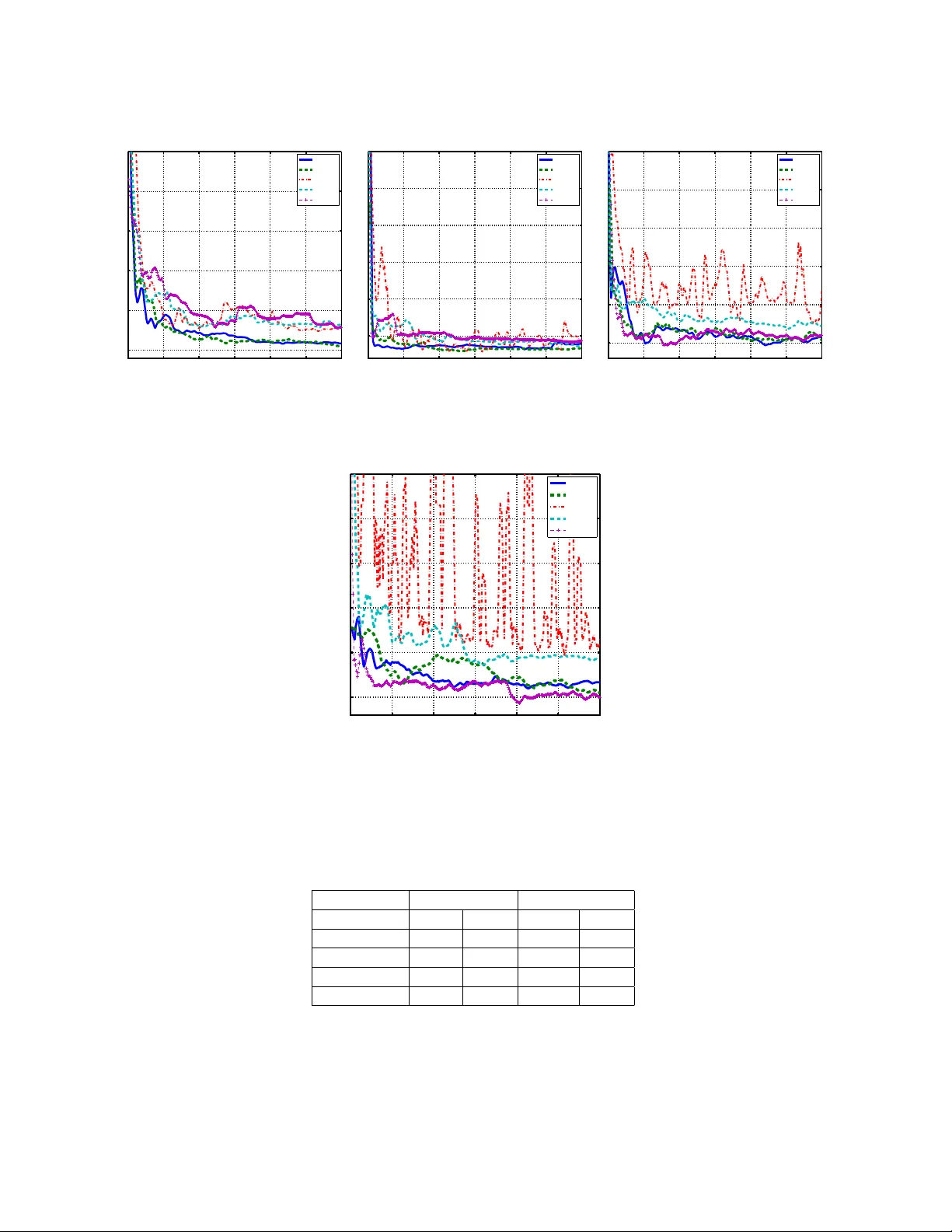
UP AL: Un biased P o ol Based Activ e Learning Ra vi Gan ti, Alexander Gra y Sc ho ol of Computational Science & Engineering, Georgia T ec h gmra vi2003@gatech.edu, agra y@cc.gatech.edu Octob er 1, 2018 Abstract In this pap er we address the problem of po ol based activ e learning, and provide an algorithm, called UP AL, that w orks by minimizing the un biased estimator of the risk of a hypothesis in a given h yp othesis space. F or the space of linear classifiers and the squared loss w e show that UP AL is equiv alen t to an ex- p onen tially w eighted a verage forecaster. Exploiting some recent results regarding the sp ectra of random matrices allo ws us to establish consistency of UP AL when the true h yp othesis is a linear h yp othesis. Em- pirical comparison with an active learner implemen tation in V owpal W abbit, and a previously prop osed p ool based active learner implementation show goo d empirical p erformance and b etter scalabilit y . 1 In tro duction In the problem of binary classification one has a distribution D on the domain X × Y ⊆ R d × {− 1 , +1 } , and access to a sampling oracle, which provides us i.i.d. lab eled samples S = { ( x 1 , y 1 ) , . . . , ( x n , y n ) } . The task is to learn a classifier h , whic h predicts well on unseen points. F or certain problems the cost of obtaining lab eled samples can b e quite exp ensiv e. F or instance consider the task of sp eec h recognition. Lab eling of sp eec h utterances needs trained linguists, and can b e a fairly tedious task. Similarly in information extraction, and in natural language pro cessing one needs exp ert annotators to obtain lab eled data, and gathering huge amoun ts of lab eled data is not only tedious for the exp erts but also exp ensiv e. In such cases it is of interest to design learning algorithms, which need only a few lab eled examples for training, and also guarantee go od p erformance on unseen data. Supp ose we are given a lab eling oracle O , whic h when queried with an unlabeled p oin t x returns the lab el y of x . Activ e learning algorithms query this oracle as few times as p ossible and learn a pro v ably go o d h yp othesis from these lab eled samples. Broadly sp eaking activ e learning (AL) algorithms can b e classified in to three kinds, namely mem b ership query (MQ) based algorithms, stream based algorithms and po ol based algorithms. All these three kinds of AL algorithms query the oracle O for the lab el of the p oin t, but differ in the nature of the queries. In MQ based algorithms the active learner can query for the lab el of a p oin t in the input space X , but this query might not necessarily b e from the supp ort of the marginal distribution D X . With h uman annotators MQ algorithms might work p o orly as was demonstrated by Lang and Baum in the case of handwritten digit recognition (1992), where the annotators were faced with the awkw ard situation of lab eling semantically meaningless images. Stream based AL algorithms (Cohn et al., 1994; Chu et al., 2011) sample a p oin t x from the marginal distribution D X , and decide on the fly whether to query O for the lab el of x ? Stream based AL algorithms tend to b e computationally efficient, and most appropriate when the underlying distribution changes with time. P o ol based AL algorithms assume that one has access to a large p ool P = { x 1 , . . . , x n } of unlab eled i.i.d. examples sampled from D X , and given budget constraints B , the maxim um num b er of p oin ts they are allo wed to query , query the most informative set of p oin ts. Both p ool based AL algorithms, and stream based AL algorithms ov ercome the problem of a wkw ard queries, whic h MQ based algorithms face. How ever in our experiments we discov ered that stream based AL algorithms tend to query more p oin ts than necessary , and hav e p o orer learning rates when compared to p o ol based AL algorithms. 1 1.1 Con tributions. 1. In this pap er w e prop ose a po ol based active learning algorithm called UP AL, which giv en a hypothesis space H , and a margin based loss function φ ( · ) minimizes a prov ably unbiased estimator of the risk E [ φ ( y h ( x ))]. While un biased estimators of risk hav e been used in stream based AL algorithms, no suc h estimators hav e b een introduced for p ool based AL algorithms. W e do this b y using the idea of imp ortance weigh ts introduced for AL in Beygelzimer et al. (2009). Roughly sp eaking UP AL pro ceeds in rounds and in each round puts a probability distribution o ver the entire p o ol, and samples a p oin t from the p o ol. It then queries for the lab el of the p oint. The probability distribution in each round is determined by the current active learner obtained by minimizing the imp ortance weigh ted risk ov er H . Sp ecifically in this pap er we shall b e concerned with linear hypothesis spaces, i.e. H = R d . 2. In theorem 2 (Section 2.1) we show that for the squared loss UP AL is equiv alent to an exp onen tially w eighted a verage (EW A) forecaster commonly used in the problem of learning with exp ert advice (Cesa- Bianc hi and Lugosi, 2006). Precisely we show that if each h yp othesis h ∈ H is considered to be an exp ert and the imp ortance weigh ted loss on the currently lab eled part of the p ool is used as an estimator of the risk of h ∈ H , then the hypothesis learned by UP AL is the same as an EW A forecaster. Hence UP AL can b e seen as pruning the hypothesis space, in a soft manner, b y placing a probability distribution that is determined by the imp ortance weigh ted loss of each classifier on the currently lab eled part of the p ool. 3. In section 3 we prov e consistency of UP AL with the squared loss, when the true underlying hypothesis is a linear hypothesis. Our pro of emplo ys s ome elegant results from random matrix theory regarding eigen v alues of sums of random matrices (Hsu et al., 2011a,b; T ropp, 2010). While it should b e p ossible to improv e the constants and exp onen t of dimensionality inv olved in n 0 ,δ , T 0 ,δ , T 1 ,δ used in theorem 3, our results qualitativ ely provide us the insight that the the lab el complexity with the squared loss will dep end on the condition num ber, and the minimum eigenv alue of the cov ariance matrix Σ. This kind of insight, to our knowledge, has not b een provided b efore in the literature of activ e learning. 4. In section 5 we pro vide a thorough empirical analysis of UP AL comparing it to the active learner implemen tation in V o wpal W abbit (VW) (Langford et al., 2011), and a batch mo de active learning algorithm, which we shall call as BMAL (Hoi et al., 2006). These exp erimen ts demonstrate the p ositive impact of imp ortance weigh ting, and the b etter p erformance of UP AL ov er the VW implementation. W e also empirically demonstrate the scalability of UP AL o ver BMAL on the MNIST dataset. When w e are required to query a large n umber of p oin ts UP AL is upto 7 times faster than BMAL. 2 Algorithm Design A go od active learning algorithm needs to take into account the fact that the p oin ts it has queried might not reflect the true underlying marginal distribution. This problem is similar to the problem of dataset shift (Quinonero e t al., 2008) where the train and test distributions are p otentially differen t, and the learner needs to take into account this bias during the learning pro cess. One approach to this problem is to use imp ortance w eights, where during the training process instead of w eighing all the points equally the algorithm w eighs the p oin ts differently . UP AL pro ceeds in rounds, where in eac h round t , we put a probabilit y distribution { p t i } n i =1 on the entire p ool P , and sample one p oin t from this distribution. If the sampled p oin t w as queried in one of the previous rounds 1 , . . . , t − 1 then its queried lab el from the previous round is reused, else the oracle O is queried for the lab el of the p oin t. Denote by Q t i ∈ { 0 , 1 } a random v ariable that takes the v alue 1 if the p oin t x i w as queried for it’s lab el in round t and 0 otherwise. In order to guarantee that our estimate of the error rate of a hypothesis h ∈ H is unbiased we use imp ortance weigh ting, where a p oin t x i ∈ P in round t gets an importance w eight of Q t i p t i . Notice that b y definition E [ Q t i | p t i ] = 1. W e formally pro v e that importance w eighted risk is an unbiased estimator of the true risk. Let D n denote a pro duct distribution 2 on ( x 1 , y 1 ) , . . . , ( x n , y n ). Also denote by Q 1: t 1: n the collection of random v ariables Q 1 1 , . . . , Q 1 n , . . . , Q t n . Let h· , ·i denote the inner pro duct. W e hav e the following result. Theorem 1. L et ˆ L t ( h ) def = 1 nt P n i =1 P t τ =1 Q τ i p τ i φ ( y i h h, x i i ) , wher e p τ i > 0 for al l τ = 1 , . . . , t . Then E Q 1 1 ,...,Q t n , D n ˆ L t ( h ) = L ( h ) . (1) Pr o of. E Q 1: t 1: n , D n ˆ L t ( h ) = E Q 1: t 1: n , D n 1 nt n X i =1 t X τ =1 Q τ i p τ i φ ( y i h h, x i i ) = E Q 1: t 1: n , D n 1 nt n X i =1 t X τ =1 E Q τ i | Q 1: τ − 1 1: n , D n Q τ i p τ i φ ( y i h h, x i i ) = E D n 1 nt n X i =1 t X τ =1 φ ( y i h h, x i i ) = L ( w ) . The theorem guarantees that as long as the probability of querying any p oin t in the p ool in any round is non-zero ˆ L t ( h ), will b e an un biased estimator of L ( h ). How does one come up with a probability distribution on P in round t ? T o solve this problem w e resort to probabilistic uncertain ty sampling, where the p oin t whose lab el is most uncertain as p er the current hypothesis, h A,t − 1 , gets a higher probability mass. The current h yp othesis is simply the minimizer of the importance w eighted risk in H , i.e. h A,t − 1 = arg min h ∈H ˆ L t − 1 ( h ). F or any p oin t x i ∈ P , to calculate the uncertaint y of the lab el y i of x i , we first estimate η ( x i ) def = P [ y i = 1 | x i ] using h A,t − 1 , and then use the entrop y of the lab el distribution of x i to calculate the probability of querying x i . The estimate of η ( · ) in round t dep ends b oth on the current active learner h A,t − 1 , and the loss function. In general it is not p ossible to estimate η ( · ) with arbitrary con vex loss functions. Ho wev er it has b een sho wn b y Zhang (2004) that the squared, logistic and exp onential losses tend to estimate the underlying conditional distribution η ( · ). Steps 4, 11 of algorithm 1 dep end on the loss function φ ( · ) b eing used. If w e use the logistic loss i.e φ ( y z ) = ln(1 + exp( − y z )) then ˆ η t ( x ) = 1 1+exp( − y h T A,t − 1 x ) . In case of squared loss ˆ η t ( x ) = min { max { 0 , w T A,t − 1 x } , 1 } . Since the loss function is con vex, and the constraint set H is conv ex, the minimization problem in step 11 of the algorithm is a conv ex optimization problem. By design UP AL might requery p oin ts. An alternate strategy is to not allow requerying of p oin ts. Ho wev er the imp ortance weigh ted risk ma y not b e an unbiased estimator of the true risk in such a case. Hence in order to retain the un biasedness prop ert y we allow requerying in UP AL. 2.1 The case of squared loss It is interesting to lo ok at the b eha viour of UP AL in the case of squared loss where φ ( y h T x ) = (1 − y h T x ) 2 . F or the rest of the pap er w e shall denote by h A the h yp othesis returned by UP AL at the end of T rounds. W e now sho w that the prediction of h A on any x is simply the exp onentially w eighted av erage of predictions of all h in H . Theorem 2. L et z i def = T X t =1 Q t i p t i ˆ Σ z def = n X i =1 z i x i x T i v z def = n X i =1 z i y i x i c def = n X i =1 z i . Define w ∈ R d as w = R R d exp( − ˆ L T ( h )) h d h R R d exp( − ˆ L T ( h )) d h . (2) Assuming ˆ Σ z is invertible we have for any x 0 ∈ R d , w T x 0 = h T A x 0 . 3 Algorithm 1 UP AL (Input: P = { x 1 , . . . , x n , } , Loss function φ ( · ), Budget B , Lab eling Oracle O ) 1. Set n um unique queries=0, h A, 0 = 0, t = 1. while num unique queries ≤ B do 2. Set Q t i = 0 for all i = 1 , . . . , n . for x 1 , . . . , x n ∈ P do 3. Set p t min = 1 nt 1 / 4 . 4. Calculate ˆ η t ( x i ) = P [ y = +1 | x i , h A,t − 1 ]. 5. Assign p t i = p t min + (1 − np t min ) ˆ η t ( x i ) ln(1 / ˆ η t ( x ))+(1 − ˆ η t ( x i )) ln(1 / (1 − ˆ η t ( x i ))) P n j =1 ˆ η t ( x j ) ln(1 / ˆ η t ( x j ))+(1 − ˆ η t ( x j )) ln(1 / (1 − ˆ η t ( x j ))) . end for 6. Sample a p oin t (say x j ) from p t ( · ). if x j w as queried previously then 7. Reuse its previously queried lab el y j . else 8. Query oracle O for its lab el y j . 9. n um unique queries ← n um unique queries+1. end if 10. Set Q t j = 1. 11. Solv e the optimization problem: h A,t = arg min h ∈H P n i =1 P t τ =1 Q τ i p τ i φ ( y i h T x i ). 12. t ← t + 1. end while 13. Return h A def = h A,t Pr o of. By elementary linear algebra one can establish that h A = ˆ Σ − 1 z v z (3) ˆ L T ( h ) = ( h − ˆ Σ − 1 z v z ) ˆ Σ z ( h − ˆ Σ − 1 z v − z ) . (4) Using standard integrals w e get Z def = Z R d exp( − ˆ L T ( h )) d h = exp( − c − v T z ˆ Σ − 1 z v z ) √ π d q det( ˆ Σ − 1 z ) . (5) In order to calculate w T x 0 , it is no w enough to calculate the integral I def = Z R d exp( − ˆ L T ( h )) h T x 0 d w . T o solve this integral we pro ceed as follo ws. Define I 1 = R R d exp( − ˆ L T ( h )) h T x 0 d h . By simple algebra we get I = Z R d exp( − w T ˆ Σ z w + 2 w T v z − c ) w T x 0 d w (6) = exp( − c − v T z ˆ Σ − 1 z v z ) I 1 . (7) 4 Let a = h − ˆ Σ − 1 z v z . W e then get I 1 = Z R d h T x 0 exp  − ( h − ˆ Σ − 1 z v z ) ˆ Σ z ( h − ˆ Σ − 1 z v z )  d h = Z R d ( a T x 0 + v T z ˆ Σ − 1 z x 0 ) exp( − a T ˆ Σ z a ) d a = Z R d ( a T x 0 ) exp( − a T ˆ Σ z a ) d a | {z } I 2 + Z R d v T z ˆ Σ − 1 z x 0 exp( − a T ˆ Σ z a ) d a | {z } I 3 . Clearly I 2 b eing the in tegrand of an o dd function ov er the entire space calculates to 0. T o calculate I 3 w e shall substitute ˆ Σ z = S S T , where S  0. Suc h a decomp osition is p ossible since ˆ Σ z  0. No w define z = S T a . W e get I 3 = v T z ˆ Σ − 1 z x 0 Z exp( − z T z ) det( S − 1 ) d z (8) = v T z ˆ Σ − 1 z x 0 det( S − 1 ) √ π d . (9) Using equations (7, 8, 9) we get I = ( √ π ) d v T z ˆ Σ − 1 z x 0 det( S − 1 ) exp( − c − v T z ˆ Σ − 1 z v z ) . (10) Hence we get w T x 0 = v T z ˆ Σ − 1 z x 0 det( S − 1 ) p det( M − 1 ) = v T z ˆ Σ − 1 z x 0 = h T A x 0 , where the p en ultimate equality follo ws from the fact that det( ˆ Σ − 1 z ) = 1 / det( ˆ Σ z ) = 1 / (det( S S T )) = 1 / (det( S )) 2 , and the last equality follows from equation 3. Theorem 2 is instructive. It tells us that assuming that the matrix ˆ Σ z is inv ertible, h A is the same as an exp onen tially w eighted a v erage of all the h yp othesis in H . Hence one can view UP AL as learning with expert advice, in the sto c hastic setting, where each individual h yp othesis h ∈ H is an exp ert, and the exp onen tial of ˆ L T is used to weigh the hypothesis in H . Suc h forecasters ha ve b een commonly used in learning with exp ert advice. This also allows us to interpret UP AL as pruning the hypothesis space in a soft wa y via exp onential w eighting, where the hypothesis that has suffered more cumulativ e loss gets lesser weigh t. 3 Bounding the excess risk It is natural to ask if UP AL is consistent? That is will UP AL do as w ell as the optimal hypothesis in H as n → ∞ , T → ∞ ? W e answer this question in affirmative. W e shall analyze the excess risk of the hypothesis returned by our active learner, denoted as h A , after T rounds when the loss function is the squared loss. The prime motiv ation for using squared loss o ver other loss functions is that squared losses yield closed form estimators, which can then b e elegantly analyzed using results from random matrix theory (Hsu et al., 2011a,b; T ropp, 2010). It should b e p ossible to extend these results to other loss functions suc h as the logistic loss, or exp onen tial loss using results from empirical pro cess theory (v an de Geer, 2000). 3.1 Main result Theorem 3. L et ( x 1 , y 1 ) , . . . ( x n , y n ) b e sample d i.i.d fr om a distribution. Supp ose assumptions A0-A3 hold. L et δ ∈ (0 , 1) , and supp ose n ≥ n 0 ,δ , T ≥ max { T 0 ,δ , T 1 ,δ } . With pr ob ability atle ast 1 − 10 δ the exc ess risk of the active le arner r eturne d by UP AL after T r ounds is L ( h A ) − L ( β ) = O  1 n + n √ T ( d + 2 p d ln(1 /δ ) + 2 ln(1 /δ ))  . 5 3.2 Assumptions, and Notation. A0 (Inv ertibility of Σ) The data cov ariance matrix Σ is inv ertible. A1 (Statistical lev erage condition) There exists a finite γ 0 ≥ 1 suc h that almost surely || Σ − 1 / 2 x || ≤ γ 0 √ d. A2 There exists a finite γ 1 ≥ 1 suc h that E [exp( α T x )] ≤ exp  || α || 2 γ 2 1 2  . A3 (Linear hypothesis) W e shall as sume that y = β T x + ξ ( x ), where ξ ( x ) ∈ [ − 2 , +2] is additive noise with E [ ξ ( x ) | x ] = 0. Assumption A0 is necessary for the problem to b e well defined. A1 has b een used in recent literature to analyze linear regression under random design and is a Bernstein like condition (Rokhlin and T ygert, 2008). A2 can b e seen as a softer form of b oundedness condtion on the supp ort of the distribution. In particular if the data is b ounded in a d-dimensional unit cub e then it suffices to take γ 1 = 1 / 2. It ma y b e p ossible to satisfy A3 by mapping data to kernel spaces. Though p opularly used kernels such as Gaussian kernel map the data to infinite dimensional spaces, a finite dimensional approximation of suc h kernel mappings can b e found by the use of random features (Rahimi and Rec ht, 2007). Notation. 1. h A is the active learner outputted by our active learning algorithm at the end of T rounds. 2. ∀ i = 1 , . . . , n : z i def = T X t =1 Q t i p t i ˆ Σ z def = n X i =1 z i x i x T i ψ z def = n X i =1 z i ξ ( x i ) x i ˆ Σ def = 1 n n X i =1 x i x T i Σ def = E [ xx T ] ˆ Σ z def = n X i =1 z i x i x T i n 0 ,δ def = 7200 d 2 γ 4 0 ( d ln(5) + ln(10 /δ )) T 1 ,δ def = 12 + 512 √ 2 d 8 / 3 γ 16 / 3 0 ln 4 / 3 ( d/δ ) T 0 ,δ def = γ 16 / 3 1 d 8 / 3 ln 4 / 3 ( d/δ ) ln 8 / 3 ( n/δ ) λ 8 / 3 min (Σ) + 4 ln( d/δ ) λ max (Σ) λ min (Σ) , where δ ∈ (0 , 1). 3.3 Ov erview of the pro of The excess risk of a hypothesis h ∈ H is defined as L ( h ) − L ( β ) = E x,y ∼D [( y − h T x ) 2 − ( y − β T x ) 2 ]. Our aim is to pro vide high probability b ounds for the excess risk, where the probability measure is w.r.t the sampled p oin ts ( x 1 , y 1 ) , . . . , ( x n , y n ) , Q 1 1 , . . . , Q T n . The pro of pro ceeds as follows. 1. In lemma 1, assuming that the matrices ˆ Σ z , ˆ Σ are inv ertible we upp er b ound the excess risk as the pro duct || Σ 1 / 2 ˆ Σ − 1 z Σ 1 / 2 || 2 || Σ − 1 / 2 ˆ Σ 1 / 2 || 2 || ˆ Σ − 1 / 2 ψ z || 2 . The prime motiv ation in doing so is that b ounding suc h “squared norm” terms can b e reduced to b ounding the maximum eigenv alue of random matrices, whic h is a well studied problem in random matrix theory . 6 2. In lemma 5 we provide an upp er b ound for || Σ − 1 / 2 ˆ Σ 1 / 2 || 2 . T o do this we use the simple fact that the matrix 2-norm of a p ositiv e semidefinite matrix is nothing but the maximum eigenv alue of the matrix. With this obsercation, and by exploiting the structure of the matrix ˆ Σ, the problem reduces to giving probabilistic upp er b ounds for maximum eigenv alue of a sum of random rank-1 matrices. Theorem 5 pro vides us with a to ol to pro ve such b ounds. 3. In lemma 6 we b ound || Σ 1 / 2 ˆ Σ − 1 z Σ 1 / 2 || 2 . The pro of is in the same spirit as in lemma 5, ho wev er the resulting probability problem is that of bounding the maxim um eigenv alue of a sum of random matrices, whic h are not necessarily rank-1. Theorem 6 provides us with Bernstein type b ounds to analyze the eigen v alues of sums of random matrices. 4. In lemma 7 we b ound the quantit y || ˆ Σ − 1 / 2 ψ z || 2 . Notice that here we are b ounding the squared norm of a random vector. Theorem 4 provides us with a to ol to analyze such quadratic forms under the assumption that the random vector has sub-Gaussian exp onen tial moments b ehaviour. 5. Finally all the abov e steps were conditioned on the in vertibilit y of the random matrices ˆ Σ , ˆ Σ z . W e pro vide conditions on n, T (this explains why w e defined the quantities n 0 ,δ , T 0 ,δ , T 1 ,δ ) which guaran tee the inv ertibility of ˆ Σ , ˆ Σ z . Suc h problems b oil down to calculating low er b ounds on the minimum eigen v alue of the random matrices in question, and to establish such low er b ounds we once again use theorems 5, 6. 3.4 F ull Pro of W e shall now provide a wa y to b ound the excess risk of our active learner hypothesis. Supp ose h A w as the h yp othesis represented by the activ e learner at the end of the T rounds. By the definition of our active learner and the definition of β w e get h A = arg min h ∈H n X i =1 T X t =1 Q t i p t i ( y i − h T x i ) 2 = n X i =1 z i ( y i − h T x i ) 2 = ˆ Σ − 1 z v z (11) β = arg min h ∈H E ( y − β T x ) 2 = Σ − 1 E [ y x ] . (12) Lemma 1. Asumme ˆ Σ z , ˆ Σ ar e b oth invertible, and assumption A0 applies. Then the exc ess risk of the classifier after T r ounds of our active le arning algorithm is given by L ( h A ) − L ( β ) ≤ || Σ 1 / 2 ˆ Σ − 1 z Σ 1 / 2 || 2 || Σ − 1 / 2 ˆ Σ 1 / 2 || 2 || ˆ Σ − 1 / 2 ψ z || 2 . (13) Pr o of. L ( h A ) − L ( β ) = E [( y − h T A x ) 2 − ( y − β T x ) 2 ] = E x,y [ h T A xx T h A − 2 y h T A x − β T xx T β + 2 y β T x ] = h T A Σ h A − 2 h T A E [ xy ] − β T Σ β + 2 β T Σ β [Since Σ β = E [ y x ]] = h T A Σ h A − β T Σ β − 2 h T A Σ β + 2 β T Σ β = h T A Σ h A + β T Σ β − 2 h T A Σ β = || Σ 1 / 2 ( h A − β ) || 2 . (14) W e shall next b ound the quantit y || h A − β || which will b e used to b ound the excess risk in Equation ( 14). T o do this we shall use assumption A3 along with the definitions of h A , β . W e hav e the following chain of 7 inequalities. h A = ˆ Σ − 1 z v z = ˆ Σ − 1 z n X i =1 z i y i x i = ˆ Σ − 1 z n X i =1 z i ( β T x i + ξ ( x i )) x i = ˆ Σ − 1 z n X i =1 z i x i x T i β + z i ξ ( x i ) x i = β + ˆ Σ − 1 z n X i =1 z i ξ ( x i ) x i = β + ˆ Σ − 1 z ψ z . (15) Using Equations 14,15 we get the following series of inequalities for the excess risk b ound L ( h A ) − L ( β ) = || Σ 1 / 2 ˆ Σ − 1 z ψ z || 2 = || Σ 1 / 2 ˆ Σ − 1 z ˆ Σ 1 / 2 ˆ Σ − 1 / 2 ψ z || 2 = || Σ 1 / 2 ˆ Σ − 1 z Σ 1 / 2 Σ − 1 / 2 ˆ Σ 1 / 2 ˆ Σ − 1 / 2 ψ z || 2 (16) ≤ || Σ 1 / 2 ˆ Σ − 1 z Σ 1 / 2 || 2 || Σ − 1 / 2 ˆ Σ 1 / 2 || 2 || ˆ Σ − 1 / 2 ψ z || 2 . The decomposition in lemma 1 assumes that b oth ˆ Σ z , ˆ Σ are in v ertible. Before w e can establish conditions for the matrices ˆ Σ z , ˆ Σ to b e inv ertible we need the following elementary result. Prop osition 1. F or any arbitr ary α ∈ R d , under assumption A1 we have E [exp( α T Σ − 1 / 2 x )] ≤ 5 exp  3 dγ 2 0 || α || 2 2  . (17) Pr o of. F rom Cauch y-Sch warz inequality and A1 we get −|| α || γ 0 √ d ≤ −|| α || || Σ − 1 / 2 x || ≤ α T Σ − 1 / 2 x ≤ || α || || Σ − 1 / 2 x || ≤ || α || γ 0 √ d. (18) Also E [ α T Σ − 1 / 2 x ] ≤ || α || γ 0 √ d . Using Ho effding’s lemma we get E [exp( α T Σ − 1 / 2 x )] ≤ exp  || α || γ 0 √ d + || α || 2 dγ 2 0 2  (19) ≤ 5 exp(3 || α || 2 dγ 2 0 / 2) . The following lemma will b e useful in b ounding the terms || Σ 1 / 2 ˆ Σ − 1 z Σ 1 / 2 || , || Σ − 1 / 2 ˆ Σ 1 / 2 || 2 . Lemma 2. L et J def = P n i =1 Σ − 1 / 2 x i x T i Σ − 1 / 2 . L et n ≥ n 0 ,δ . Then the fol lowing ine qualities hold sep ar ately with pr ob ability atle ast 1 − δ e ach λ max ( J ) ≤ n + 6 dnγ 2 0 " r 32( d ln(5) + ln(10 /δ )) n + 2( d ln(5) + ln(10 /δ )) n # ≤ 3 n/ 2 (20) λ min ( J ) ≥ n − 6 dnγ 2 0 " r 32( d ln(5) + ln(10 /δ )) n + 2( d ln(5) + ln(10 /δ )) n # ≥ n/ 2 . (21) 8 Pr o of. Notice that E [Σ − 1 / 2 x i x T i Σ − 1 / 2 ] = I . F rom Prop osition 1 we ha ve E [exp( α T Σ − 1 / 2 x )] ≤ 5 exp(3 || α || 2 dγ 2 0 / 2). By using theorem 5 we get with probability atleast 1 − δ : λ max 1 n n X i =1 (Σ − 1 / 2 x i )(Σ − 1 / 2 x i ) T ! ≤ 1 + 6 dγ 2 0 " r 32( d ln(5) + ln(2 /δ )) n + 2( d ln(5) + ln(2 /δ )) n # . (22) Put n ≥ n 0 ,δ to get the desired result. The low er b ound on λ min is also obtained in the same w ay . Lemma 3. L et n ≥ n 0 ,δ . With pr ob ability atle ast 1 − δ sep ar ately we have ˆ Σ  0 , λ min ( ˆ Σ) ≥ 1 2 λ min (Σ) , λ max ( ˆ Σ) ≤ 3 2 λ max (Σ) . Pr o of. Using lemma 2 we get for n ≥ n 0 ,δ with probability atleast 1 − δ , λ min ( J ) ≥ 1 / 2 and with probability atleast 1 − δ , λ max (Σ) ≤ 3 / 2. Finally since Σ 1 / 2 J Σ 1 / 2 = ˆ Σ, and J  0 , Σ  0, we get ˆ Σ  0. F urther we ha ve the following upp er b ound with probability atleast 1 − δ : λ max ( ˆ Σ) = || Σ 1 / 2 J Σ 1 / 2 || (23) ≤ || Σ 1 / 2 || 2 || J || (24) ≤ || Σ || || J || (25) = λ max (Σ) λ max ( J ) (26) ≤ 3 2 λ max (Σ) , (27) where in the last step we used the upp er b ound on λ max ( J ) provided by lemma 2. Similarly we hav e the follo wing lo wer b ound with probability atleast 1 − δ λ min ( ˆ Σ) = 1 λ max (Σ − 1 / 2 J − 1 Σ − 1 / 2 ) (28) = 1 || Σ − 1 / 2 J − 1 Σ − 1 / 2 || (29) ≥ 1 || Σ − 1 || || J − 1 || || Σ − 1 / 2 || (30) = λ min (Σ) λ min ( J ) (31) ≥ λ min (Σ) 2 , (32) where in the last step we used the low er b ound on λ min ( J ) provided by lemma 2. The following prop osition will b e useful in proving lemma 4. Prop osition 2. L et δ ∈ (0 , 1) . Under assumption A2, with pr ob ability atle ast 1 − δ , P n i =1 || x i || 4 ≤ 25 γ 4 1 d 2 ln 2 ( n/δ ) Pr o of. F rom A2 we hav e E [exp( α T x )] ≤ exp( || α || 2 γ 2 1 2 ). No w applying theorem 4 with A = I d w e get P [ || x i || 2 ≤ dγ 2 1 + 2 γ 2 1 p d ln(1 /δ ) + 2 γ 2 1 ln(1 /δ )] ≥ 1 − δ . (33) The result now follo ws b y the union b ound. Lemma 4. L et δ ∈ (0 , 1) . F or T ≥ T 0 ,δ , with pr ob ability atle ast 1 − 4 δ we have λ min ( ˆ Σ z ) ≥ nT λ min (Σ) 4 > 0 . Henc e ˆ Σ z is invertible. 9 Pr o of. The proof uses theorem 6. Let M 0 t def = P n i =1 Q t i p t i x i x T i , so that ˆ Σ z = P T t =1 M 0 t . Now E t M 0 t = n ˆ Σ. Define R 0 t def = n ˆ Σ − M 0 t , so that E t R 0 t = 0. W e shall apply theorem 6 to the random matrix P R 0 t . In order to do so we need upp er b ounds on λ max ( R 0 t ) and λ max ( 1 T P T t =1 E t R 0 2 t ). Let n ≥ n 0 ,δ . Using lemma 3 we get with probabilit y atleast 1 − δ λ max ( R 0 t ) = λ max ( n ˆ Σ − M 0 t ) ≤ λ max ( n ˆ Σ) ≤ 3 nλ max (Σ) 2 def = b 2 . (34) λ max " 1 T T X t =1 E t R 0 2 t # = 1 T λ max " T X t =1 E t ( n ˆ Σ − M 0 t ) 2 # (35) = 1 T λ max ( − n 2 T ˆ Σ 2 + T X t =1 E t n X i =1 Q t i ( p t i ) 2 ( x i x T i ) 2 ) (36) = 1 T λ max ( − n 2 T ˆ Σ 2 + T X t =1 n X i =1 1 p t i ( x i x T i ) 2 ) (37) ≤ 1 T λ max ( n X i =1 T X t =1 1 p t i ( x i x T i ) 2 ) − n 2 λ 2 min ( ˆ Σ) (38) ≤ nT 1 / 4 λ max ( n X i =1 ( x i x T i ) 2 ) (39) ≤ nT 1 / 4 n X i =1 λ 2 max ( x i x T i ) (40) = nT 1 / 4 n X i =1 || x i || 4 (41) ≤ 25 γ 4 1 d 2 n 2 T 1 / 4 ln 2 ( n/δ ) def = σ 2 2 . (42) Equation 36 follows from Equation 35 by the definition of M 0 t and the fact that at any given t only one p oin t is queried i.e. Q t i Q t j = 0 for a given t . Equation 37 follows from equation 36 since E t Q t i = p t i . Equation 38 follo ws from Equation 37 b y W eyl’s inequality . Equation 39 follows from Equation 38 by substituting p t min in place of p t i . Equation 40 follows from Equation 39 by the use of W eyl’s inequality . Equation 41 follows from Equation 40 by using the fact that if p is a vector then λ max ( pp T ) = || p || 2 . Equation 42 follows from Equation 41 b y the use of prop osition 2. Notice that this step is a stochastic inequality and holds with probabilit y atleast 1 − δ . Finally applying theorem 6 we hav e P " λ max ( 1 T T X t =1 R 0 t ) ≤ r 2 σ 2 2 ln( d/δ ) T + b 2 ln( d/δ ) T # ≥ 1 − δ (43) = ⇒ P " λ max ( n ˆ Σ − 1 T T X t =1 M 0 t ) ≤ r 2 σ 2 2 ln( d/δ ) T + b 2 ln( d/δ ) T # ≥ 1 − δ (44) = ⇒ P " λ min ( n ˆ Σ) − 1 T λ min T X t =1 M 0 t ! ≤ r 2 σ 2 2 ln( d/δ ) T + b 2 ln( d/δ ) T # ≥ 1 − δ (45) 10 Substituting for σ 2 , b 2 , rearranging the inequalities, and using lemma 3 to lo wer b ound λ min ( ˆ Σ) we get P " λ min ( T X t =1 M 0 t ) ≥ T λ min ( n ˆ Σ) − q 2 T σ 2 2 ln( d/δ ) − b 2 ln( d/δ ) # ≥ 1 − δ = ⇒ P " λ min ( T X t =1 M 0 t ) ≥ nT λ min (Σ) 2 − q 2 T σ 2 2 ln( d/δ ) − b 2 ln( d/δ ) # ≥ 1 − 2 δ = ⇒ P " λ min ( T X t =1 M 0 t ) ≥ nT λ min (Σ) 2 − 5 √ 2 γ 2 1 dnT 5 / 8 p ln( d/δ ) ln( n/δ ) − n ln( d/δ ) λ max (Σ) 2 # ≥ 1 − 4 δ F or T ≥ T 0 ,δ with probability atleast 1 − 4 δ , λ min P T t =1 M 0 t = λ min ( ˆ Σ z ) ≥ nT λ min (Σ) 4 . Lemma 5. F or n ≥ n 0 ,δ with pr ob ability atle ast 1 − δ over the r andom sample x 1 , . . . , x n || Σ − 1 / 2 ˆ Σ 1 / 2 || 2 ≤ 3 / 2 . (46) Pr o of. || Σ − 1 / 2 ˆ Σ 1 / 2 || 2 = || ˆ Σ 1 / 2 Σ − 1 / 2 || 2 (47) = λ max (Σ − 1 / 2 ˆ ΣΣ − 1 / 2 ) (48) = λ max 1 n n X i =1 (Σ − 1 / 2 x i )(Σ − 1 / 2 x i ) T ! (49) = λ max  J n  (50) ≤ 3 / 2 (51) where in the first equality w e used the fact that || A || = || A T || for a square matrix A , and || A || 2 = λ max ( A T A ), and in the last step we used lemma 2. Lemma 6. Supp ose ˆ Σ z is invertible. Given δ ∈ (0 , 1) , for n ≥ n 0 ,δ , and T ≥ max { T 0 ,δ , T 1 ,δ } with pr ob ability atle ast 1 − 3 δ over the samples || Σ 1 / 2 ˆ Σ − 1 z Σ 1 / 2 || 2 ≤ 400 n 2 T 2 . Pr o of. The pro of of this lemma is very similar to the pro of of lemma 4. F rom lemma 4 for n ≥ n 0 ,δ , T ≥ T 0 ,δ with probabilit y atleast 1 − δ , ˆ Σ z  0. Using the assumption that Σ  0, w e get Σ 1 / 2 ˆ Σ − 1 z Σ 1 / 2  0. Hence || Σ 1 / 2 ˆ Σ − 1 z Σ 1 / 2 || = λ max (Σ 1 / 2 ˆ Σ − 1 z Σ 1 / 2 ) = 1 λ min (Σ − 1 / 2 ˆ Σ z Σ − 1 / 2 ) . Hence it is enough to pro vide a low er b ound on the smallest eigen v alue of the symmetric p ositiv e definite matrix Σ − 1 / 2 ˆ Σ z Σ − 1 / 2 . λ min (Σ − 1 / 2 ˆ Σ z Σ − 1 / 2 ) = λ min n X i =1 z i Σ − 1 / 2 x i x T i Σ − 1 / 2 ! = λ min ( T X t =1 n X i =1 Q t i p t i Σ − 1 / 2 x i x T i Σ − 1 / 2 | {z } def = M t ) = λ min T X t =1 M t ! . 11 Define R t def = J − M t . Clearly E t [ M t ] = J , and hence E [ R t ] = 0. F rom W eyl’s inequality we hav e λ min ( J ) + λ max  − 1 T P T t =1 M t  ≤ λ max ( 1 T P T t =1 R t ). No w applying theorem 6 on P R t w e get with probability atleast 1 − δ λ min ( J ) + λ max − 1 T T X t =1 M t ! ≤ λ max 1 T T X t =1 R t ! ≤ r 2 σ 2 1 ln( d/δ ) T + b 1 ln( d/δ ) 3 T , (52) where λ max 1 T T X t =1 J − M t ! ≤ b 1 (53) λ max 1 T T X t =1 E t ( J − M t ) 2 ! ≤ σ 2 1 (54) Rearranging Equation (52) and using the fact that λ max ( − A ) = − λ min ( A ) we get with probability atleast 1 − δ , λ min T X t =1 M t ! ≥ T λ min ( J ) − q 2 T σ 2 1 ln( d/δ ) − b 1 ln( d/δ ) 3 . (55) Using W eyl’s inequalit y (Horn and Johnson, 1990) w e hav e λ max ( 1 T P T t =1 J − M t ) ≤ λ max ( J ) ≤ 3 n 2 with probabilit y atleast 1 − δ , where in the last step we used lemma (2). Let b 1 def = 3 n 2 . T o calculate σ 2 1 w e pro ceed as follows. λ max 1 T T X t =1 E t ( J − M t ) 2 ! = 1 T λ max T X t =1 E t ( M 2 t ) − J 2 ! (56) ≤ 1 T λ max T X t =1 E t M 2 t ! (57) = 1 T λ max   T X t =1 E t n X i =1 Q t i p t i Σ − 1 / 2 x i x T i Σ − 1 / 2 ! 2   (58) = 1 T λ max T X t =1 E t n X i =1 Q t i ( p t i ) 2 (Σ − 1 / 2 x i x T i Σ − 1 / 2 ) 2 ! (59) = 1 T λ max T X t =1 n X i =1 1 p t i (Σ − 1 / 2 x i x T i Σ − 1 / 2 ) 2 ! (60) ≤ 1 T T X t =1 n X i =1 1 p t i || Σ − 1 / 2 x i || 4 (61) ≤ d 2 γ 4 0 T n X i =1 T X t =1 1 p t i (62) ≤ nd 2 γ 4 0 T T X t =1 1 p t min (63) ≤ n 2 d 2 γ 4 0 T 1 / 4 def = σ 2 1 . (64) Equation 57 follows from Equation 56 by using W eyl’s inequalit y and the fact that J 2  0. Equation 59 follo ws from Equation 58 since only one p oin t is queried in every round and hence for any given t, i 6 = j 12 w e ha ve Q t i Q t j = 0, and hence all the cross terms disapp ear when w e expand the square. Equation (60) follo ws from Equation (59) by using the fact that E t Q t = p t . Equation (61) follows from Equation (60) by W eyl’s inequalit y and the fact that the maximum eigenv alue of a rank-1 matrix of the form v v T is || v || 2 . Equation (62) follows from Equation (61) by using assumption A1. Equation 64 follows from Equation (63) b y our choice of p t min = 1 n √ t . Substituting the v alues of σ 2 1 , b 1 in 55, using lemma 2 to low er b ound λ min ( J ), and applying union b ound to sum up all the failure probabilities we get for n ≥ n 0 ,δ , T ≥ max { T 0 ,δ , T 1 ,δ } with probability atleast 1 − 3 δ , λ min T X t =1 M t ! ≥ T λ min ( J ) − q 2 T 5 / 4 n 2 d 2 γ 4 0 ln( d/δ ) − 3 n/ 2 ≥ nT 2 − √ 2 T 5 / 8 ndγ 2 0 p ln( d/δ ) − 3 n/ 2 ≥ nT / 4 . The only missing piece in the pro of is an upp er b ound for the quantit y || ˆ Σ − 1 / 2 ψ z || 2 . The next lemma pro vides us with an upp er b ound for this quantit y . Lemma 7. Supp ose ˆ Σ is invertible. L et δ ∈ (0 , 1) . With pr ob ability atle ast 1 − δ we have || ˆ Σ − 1 / 2 ψ z || 2 ≤ (2 nT 2 + 56 n 3 T √ T )( d + 2 p d ln(1 /δ ) + 2 ln(1 /δ )) . Pr o of. Define the matrix A ∈ R d × n as follo ws. Let the i th column of A b e the v ector ˆ Σ − 1 / 2 x i √ n , so that AA T = 1 n ˆ Σ − 1 / 2 x i x T i ˆ Σ − 1 / 2 = I d . Now || ˆ Σ − 1 / 2 ψ z || 2 = || √ nAp || 2 , where p = ( p 1 , . . . , p n ) ∈ R n and p i = ξ ( x i ) z i for i = 1 , . . . , n . Using the result for quadratic forms of subgaussian random v ectors (threorem 4) we get || Ap || 2 ≤ σ 2 (tr( I d ) + 2 p tr( I d ) ln(1 /δ ) + 2 || I d || ln(1 /δ )) = σ 2 ( d + 2 p d ln(1 /δ ) + 2 ln(1 /δ )) , (65) where for any arbitrary vector α , E [exp( α T p )] ≤ exp( || α || 2 σ 2 ). Hence all that is left to b e done is prov e that α T p has sub-Gaussian exp onen tial moments. Let D t def = n X i =1 α i ξ ( x i ) Q t i p t i − α T ξ ∀ t = 1 , . . . , T . (66) With this definition w e ha ve the following series of equalities E [exp( α T p )] = E [exp( X D t + T α T ξ )] = E h exp( T α T ξ ) E [exp( X D t ) |D n ] i . (67) Conditioned on the data, the sequence D 1 , . . . , D T , forms a martingale difference sequence. Let ξ = [ ξ ( x 1 ) , . . . , ξ ( x n )]. Notice that − α T ξ − 2 || α || p t min ≤ D t ≤ − α T ξ + 2 || α || p t min . (68) W e shall now b ound the probability of large deviations of D t giv en history up until time t . This allows us to put a b ound on the large deviations of the martingale sum P T t =1 D t . Let a ≥ 0. Using Marko v’s inequalit y w e get P [ D t ≥ a | Q 1: t − 1 1: n , D n ] ≤ min γ > 0 exp( − γ a ) E [ γ D t | Q 1: t − 1 1: n , D n ] (69) ≤ min γ > 0 exp  2 γ 2 || α || 2 ( p t min ) 2 − γ a  (70) ≤ exp  − a 2 8 || α || 2 n 2 √ t  . (71) 13 In the second step we used Ho effding’s lemma along with the b oundedness prop ert y of D t sho wn in equa- tion 68. The same upp er b ound can b e shown for the quantit y P [ D t ≤ a | Q 1: t − 1 1: n , D n ]. Applying lemma 7 w e get with probability atleast 1 − δ , conditioned on the data, w e ha ve 1 T T X t =1 D t ≤ s 448 || α || 2 n 2 ln(1 /δ ) √ T = ⇒ T X t =1 D t ≤ q 112 || α || 2 n 2 T 3 / 2 ln(1 /δ ) . (72) Hence P T t =1 D t , conditioned on data, has sub-Gaussian tails as shown ab o v e. This leads to the following conditional exp onen tial moments b ound E [exp( T X t =1 D t ) |D n ] = exp  56 || α || 2 n 2 T √ T ln(1 /δ )  . (73) Finally putting together equations 67, 73 w e get E [exp( α T p )] ≤ E exp( T α T ξ ) exp(56 || α || 2 n 2 T √ T ) ≤ exp((2 T 2 + 56 n 2 T √ T ) || α || 2 ) , (74) In the last step we exploited the fact that − 2 ≤ ξ ( x i ) ≤ 2, and hence by Ho effding lemma E [exp( α T ξ )] ≤ exp(2 || α || 2 ). This leads us to the choice of σ 2 = 2 T 2 + 56 n 2 T √ T . Substituting this v alue of σ 2 in equation 65 w e get || Ap || 2 ≤ (2 T 2 + 56 n 2 T √ T )( d + 2 p d ln(1 /δ ) + 2 ln(1 /δ )) , (75) and hence with probabilit y atleast 1 − δ , || ˆ Σ − 1 / 2 ψ z || 2 = n || Ap || 2 ≤ (2 nT 2 + 56 n 3 T √ T )( d + 2 p d ln(1 /δ ) + 2 ln(1 /δ )) . (76) W e are now ready to prov e our main result. Pr o of of the or em 3 . F or n ≥ n 0 ,δ and T ≥ max { T 0 ,δ , T 1 ,δ } from lemma 3, 4, both ˆ Σ z , and ˆ Σ are in vertible with probability atleast 1 − δ, 1 − 4 δ resp ectiv ely . Conditioned on the in v ertibility of ˆ Σ z , Σ we get from lemmas 5-7, || Σ − 1 ˆ Σ 1 / 2 || 2 ≤ 3 / 2 and || Σ 1 / 2 ˆ Σ − 1 z Σ 1 / 2 || 2 ≤ 400 /n 2 T 2 , and || ˆ Σ − 1 / 2 ψ z || 2 ≤ (2 nT 2 + 56 n 3 T 3 / 2 )( d + 2 p d ln(1 /δ ) + 2 ln(1 /δ )) with probabilit y atleast 1 − δ, 1 − 3 δ, 1 − δ resp ectiv ely . Using lemma 1 and the union b ound to add up all the failure probabilities we get the desired result. 4 Related W ork A v ariety of p ool based AL algorithms hav e b een prop osed in the literature employing v arious query strate- gies. Ho wev er, none of them use unbiased estimates of the risk. One of the simplest strategy for AL is uncertain ty sampling, where the activ e learner queries the p oin t whose lab el it is most uncertain about. This strategy has b een p opularl in text classification (Lewis and Gale, 1994), and information extraction (Settles and Crav en, 2008). Usually the uncertaint y in the lab el is calculated using certain information-theoretic cri- teria such as en tropy , or v ariance of the lab el distribution. While uncertain ty sampling has mostly b een used in a probabilistic setting, AL algorithms which learn non-probabilistic classifiers using uncertaint y sampling ha ve also been proposed. T ong et al. (2001) prop osed an algorithm in this framework where they query the p oin t closest to the current svm hyperplane. Seung et al. (1992) introduced the query-b y-committee (QBC) framework where a committee of p oten tial mo dels, whic h all agree on the curren tly lab eled data is main tained and, the p oin t where most committee members disagree is considered for querying. In order to design a committee in the QBC framework, algorithms such as query-by-bo osting, and query-by-bagging in the discriminative setting (Ab e and Mamitsuk a, 1998), sampling from a Dirichlet distribution ov er mo del parameters in the generative setting (McCallum and Nigam, 1998) hav e b een prop osed. Other frameworks include querying the p oin t, which causes the maximum exp ected reduction in error (Zhu et al., 2003; Guo and Greiner, 2007), v ariance reducing query strategies such as the ones based on optimal design (Flaherty 14 et al., 2005; Zhang and Oles, 2000). A v ery thorough literature survey of different active learning algorithms has b een done by Settles (2009). AL algorithms that are consistent and hav e prov able lab el complexity hav e b een prop osed for the agnostic setting for the 0-1 loss in recen t years (Dasgupta et al., 2007; Beygelzimer et al., 2009). The IW AL framework introduced in Beygelzimer et al. (2009) was the first AL algorithm with guarantees for general loss functions. Ho wev er the authors were unable to provide non-trivial label complexit y guaran tees for the hinge loss, and the squared loss. UP AL at least for squared losses can be seen as using a QBC based querying strategy where the committee is the entire hypothesis space, and the disagreement among the committee members is calculated using an exp onen tial weigh ting scheme. How ever unlike previously prop osed committees our committee is an infinite set, and the c hoice of the p oin t to b e queried is randomized. 5 Exp erimen tal results W e implemen ted UP AL, along with the standard passive learning (PL) algorithm, and a v ariant of UP AL called RAL (in short for random activ e learning), all using logistic loss, in matlab. The choice of logistic loss was motiv ated by the fact that BMAL was designed for logistic loss. Our matlab co des were vectorized to the maxim um p ossible extent so as to b e as efficient as p ossible. RAL is similar to UP AL, but in each round samples a p oin t uniformly at random from the currently unqueried po ol. How ever it do es not use imp ortance weigh ts to calculate an estimate of the risk of the classifier. The purp ose of implemen ting RAL w as to demonstrate the p oten tial effect of using unbiased estimators, and to c heck if the strategy of randomly querying p oin ts helps in active learning. W e also implemented a batc h mo de active learning algorithm introduced by Hoi et al. (2006) which, we shall call as BMAL. Hoi et al. in their pap er show ed sup erior empirical p erformance of BMAL ov er other comp eting p ool based active learning algorithms, and this is the primary motiv ation for choosing BMAL as a comp etitor p ool AL algorithm in this pap er. BMAL like UP AL also pro ceeds in rounds and in eac h iteration selects k examples b y minimizing the Fisher information ratio b et ween the current unqueried p ool and the queried p o ol. How ever a p oin t once queried by BMAL is never requeried. In order to tackle the high computational complexit y of optimally choosing a set of k p oints in each round, the authors suggested a monotonic submo dular approximation to the original Fisher ratio ob jective, which is then optimized by a greedy algorithm. At the start of round t + 1 when, BMAL has already queried t p oin ts in the previous rounds, in order to decide which p oin t to query next, BMAL has to calculate for each p oten tial new query a dot pro duct with all the remaining unqueried p oints. Such a calculation when done for all p ossible p otential new queries takes O ( n 2 t ) time. Hence if our budget is B , then the total computational complexity of BMAL is O ( n 2 B 2 ). Note that this calculation do es not take into account the complexity of solving an optimization problem in eac h round after having queried a p oin t. In order to further reduce the computational complexit y of BMAL in eac h round w e further restrict our search, for the next query , to a small subsample of the curren t set of unqueried p oin ts. W e set the v alue of p min in step 3 of algorithm 1 to 1 nt . In order to av oid n umerical problems we implemented a regularized version of UP AL where the term λ || w || 2 w as added to the optimization problem sho wn in step 11 of Algorithm 1. The v alue of λ is allo wed to c hange as per the curren t imp ortance weigh t of the p ool. The optimal v alue of C in VW 1 w as chosen via a 5 fold cross-v alidation, and by eyeballing for the v alue of C that ga ve the b est cost-accuracy trade-off. W e ran all our exp erimen ts on the MNIST dataset(3 Vs 5) 2 , and datasets from UCI rep ository namely Statlog, Abalone, Whitewine. Figure 1 shows the p erformance of all the algorithms on the first 300 queried p oin ts. On the MNIST dataset, on an av erage, the p erformance of BMAL is very similar to UP AL, and there is a noticeable gap in the p erformance of BMAL and UP AL ov er PL, VW and RAL. Similar results were also seen in the case of Statlog dataset, though tow ards the end the p erformance of UP AL sligh tly worsens when compared to BMAL. How ev er UP AL is still b etter than PL, VW, and RAL. 1 The parameters initial t, l w ere set to a default v alue of 10 for all of our experiments. 2 The dataset can b e obtained from http://cs.nyu.edu/ ~ roweis/data.html . W e first performed PCA to reduce the dimen- sions to 25 from 784. 15 0 50 100 150 200 250 300 5 10 15 20 25 30 UPAL BMAL VW RAL PL (a) MNIST (3 vs 5) 0 50 100 150 200 250 300 5 10 15 20 25 30 UPAL BMAL VW RAL PL (b) Statlog 0 50 100 150 200 250 300 25 30 35 40 45 50 UPAL BMAL VW RAL PL (c) Abalone 0 50 100 150 200 250 300 25 30 35 40 45 50 UPAL BMAL VW RAL PL (d) Whitewine Figure 1: Empirical p erformance of passive and active learning algorithms.The x-axis represents the num b er of p oin ts queried, and the y-axis represents the test error of the classifier. The subsample size for appro ximate BMAL implementation was fixed at 300. Sample size UP AL BMAL Time Error Time Error 1200 65 7.27 60 5.67 2400 100 6.25 152 6.05 4800 159 6.83 295 6.25 10000 478 5.85 643.17 5.85 T able 1: Comparison of UP AL and BMAL on MNIST data-set of v arying training sizes, and with the budget b eing fixed at 300. The error rate is in percentage, and the time is in seconds. 16 Budget UP AL BMAL Speedup Time Error Time Error 500 859 5.79 1973 5.33 2.3 1000 1919 6.43 7505 5.70 3.9 2000 4676 5.82 32186 5.59 6.9 T able 2: Comparison of UP AL on the entire MNIST dataset for v arying budget size. All the times are in seconds unless stated, and error rates in p ercen tage. Activ e learning is not alw ays helpful and the success story of AL depends on the match b et ween the marginal distribution and the hypothesis class. This is clearly reflected in Abalone where the p erformance of PL is b etter than UP AL atleast in the initial stages and is never significantly worse. UP AL is uniformly b etter than BMAL, though the difference in error rates is not significant. How ever the p erformance of RAL, VW are significan tly worse. Similar results were also seen in the case of Whitewine dataset, where PL outp erforms all AL algorithms. UP AL is b etter than BMAL most of the times. Even here one can witness a huge gap in the p erformance of VW and RAL ov er PL, BMAL and UP AL. One can conclude that VW though is computationally efficient has higher error rate for the same num b er of queries. The uniformly p oor p erformance of RAL signifies that querying uniformly at random do es not help. On the whole UP AL and BMAL p erform equally w ell, and we show via our next set of exp erimen ts that UP AL has significantly b etter scalabilit y , esp ecially when one has a relativ ely large budget B . 5.1 Scalabilit y results Eac h round of UP AL takes O ( n ) plus the time to solv e the optimization problem shown in step 11 in Algorithm 1. A similar optimization problem is also solved in the BMAL problem. If the cost of solving this optimization problem in step t is c opt,t , then the complexity of UP AL is O ( nT + P T t =1 c opt,t ). While BMAL tak es O ( n 2 B 2 + P T t =1 c 0 t,opt ) where c 0 t,opt is the complexity of solving the optimization problem in BMAL in round t . F or the approximate implementation of BMAL that we describ ed if the subsample size is | S | , then the complexity is O ( | S | 2 B 2 + P T t =1 c 0 t,opt ). In our first set of exp erimen ts we fix the budget B to 300, and calculate the test error and the combined training and testing time of b oth BMAL and UP AL for v arying sizes of the training set. All the exp erimen ts w ere p erformed on the MNIST dataset. T able 1 shows that with increasing sample size UP AL tends to b e more efficient than BMAL, though the gain in sp eed that we observed was at most a factor of 1.8. In the second set of scalability exp erimen ts w e fixed the training set size to 10000, and studied the effect of increasing budget. W e found out that with increasing budget size the speedup of UP AL ov er BMAL increases. In particular when the budget was 2000, UP AL is arppr oximately 7 times faster than BMAL. All our exp erimen ts were run on a dual core machine with 3 GB memory . 6 Conclusions and Discussion In this paper we prop osed the first un biased po ol based activ e learning algorithm, and show ed its goo d empirical p erformance and its ability to scale b oth with higher budget constrain ts and large dataset sizes. Theoretically we prov ed that when the true hypothesis is a linear hypothesis, we are able to recov er it with high probabilit y . In our view an imp ortan t extension of this work would b e to establish tigh ter b ounds on the excess risk. It should b e p ossible to provide upp er b ounds on the excess risk in exp ectation which are muc h sharp er than our current high probabilit y b ounds. Another theoretically in teresting question is to calculate ho w man y unique queries are made after T rounds of UP AL. This problem is similar to calculating the n um b er of non-empt y bins in the balls-and-bins mo del commonly used in the field of randomized algorithms Mot wani and Raghav an (1995), when there are n bins and T balls, with the different p oin ts in the p ool b eing the bins, and the pro cess of throwing a ball in each round b eing equiv alent to querying a p oint in each round. 17 Ho wev er since each round is, unlike standard balls-and-bins, dep enden t on the previous round we exp ect the analysis to b e more inv olved than a standard balls-and-bins analysis. References N. Ab e and H. Mamitsuk a. Query learning strategies using b oosting and bagging. In ICML , 1998. E.B. Baum and K. Lang. Query learning can w ork p oorly when a human oracle is used. In IJCNN , 1992. A. Beygelzimer, S. Dasgupta, and J. Langford. Importance w eighted active learning. In ICML , 2009. N. Cesa-Bianchi and G. Lugosi. Pr e diction, le arning, and games . Cam bridge Univ Press, 2006. W. Chu, M. Zinkevic h, L. Li, A. Thomas, and B. Tseng. Un biased online active learning in data streams. In SIGKDD , 2011. D. Cohn, L. Atlas, and R. Ladner. Improving generalization with active learning. Machine L e arning , 15(2), 1994. S. Dasgupta, D. Hsu, and C. Mon teleoni. A general agnostic active learning algorithm. NIPS , 2007. P atrick Flaherty , Michael I. Jordan, and Adam P . Arkin. Robust design of biological exp erimen ts. In Neur al Information Pr o c essing Systems , 2005. Y. Guo and R. Greiner. Optimistic active learning using mutual information. In IJCAI , 2007. S.C.H. Hoi, R. Jin, J. Zh u, and M.R. Lyu. Batch mo de active learning and its application to medical image classification. In ICML , 2006. R.A. Horn and C.R. Johnson. Matrix analysis . Cam bridge Univ Press, 1990. D. Hsu, S.M. Kak ade, and T. Zhang. An analysis of random design linear regression. A rxiv pr eprint arXiv:1106.2363 , 2011a. D. Hsu, S.M. Kak ade, and T. Zhang. Dimension-free tail inequalities for sums of random matrices. Arxiv pr eprint arXiv:1104.1672 , 2011b. J. Langford, L. Li, A. Strehl, D. Hsu, N. Karampatziakis, and M. Hoffman. V o wpal wabbit, 2011. D.D. Lewis and W.A. Gale. A sequential algorithm for training text classifiers. In SIGIR , 1994. AE Litv ak, A. P a jor, M. Rudelson, and N. T omczak-Jaegermann. Smallest singular v alue of random matrices and geometry of random p olytopes. A dvanc es in Mathematics , 195(2):491–523, 2005. A.K. McCallum and K. Nigam. Emplo ying EM and p ool-based activ e learning for text classification. In ICML , 1998. Ra jeev Motw ani and Prabhak ar Ragha v an. R andomize d Algorithms . Cam bridge Univ ersit y Press, 1st edition, August 1995. J. Quinonero, M. Sugiama, A. Sch waighofer, and N.D. Lawrence. Dataset shift in machine learning, 2008. Ali Rahimi and Benjamin Rech t. Random features for large-scale kernel machines. In Neur al Information Pr o c essing Systems , 2007. V. Rokhlin and M. Tygert. A fast randomized algorithm for ov erdetermined linear least-squares regression. Pr o c e e dings of the National A c ademy of Scienc es , 105(36):13212, 2008. 18 B. Settles and M. Crav en. An analysis of active learning strategies for sequence lab eling tasks. In EMNLP , 2008. Burr Settles. Activ e learning literature surv ey . Computer Sciences T echnical Rep ort 1648, Univ ersity of Wisconsin–Madison, 2009. H.S. Seung, M. Opp er, and H. Somp olinsky . Query by committee. In COL T , pages 287–294. ACM, 1992. O. Shamir. A v arian t of azuma’s inequality for martingales with subgaussian tail. A rxiv pr eprint arXiv:1110.2392 , 2011. S. T ong and E. Chang. Support v ector machine active learning for image retriev al. In Pr o c e e dings of the ninth ACM international c onfer enc e on Multime dia , 2001. J.A. T ropp. User-friendly tail b ounds for sums of random matrices. Arxiv pr eprint arXiv:1004.4389 , 2010. Sara v an de Geer. Empirical pro cesses in m-estimation. 2000. T. Zhang. Statistical b ehavior and consistency of classification metho ds based on conv ex risk minimization. A nnals of Statistics , 32(1), 2004. T. Zhang and F. Oles. The v alue of unlab eled data for classification problems. In ICML , 2000. Xiao jin Zhu, John Laffert y , and Zoubin Ghahramani. Com bining active learning and semi-supervised learning using gaussian fields and harmonic functions. In ICML , 2003. A Some results from random matrix theory Theorem 4. (Quadr atic forms of sub gaussian r andom ve ctors (Litvak et al., 2005; Hsu et al., 2011a)) L et A ∈ R m × n b e a matrix, and H def = AA T , and r = ( r 1 , . . . , r n ) b e a r andom ve ctor such that for some σ ≥ 0 , E [exp( α T r )] ≤ exp  || α || 2 σ 2 2  for al l α ∈ R n almost sur ely. F or al l δ ∈ (0 , 1) , P h || Ar || 2 > σ 2 tr( H ) + 2 σ 2 p tr( H 2 ) ln(1 /δ ) + 2 σ 2 || H || ln(1 /δ ) i ≤ δ. The ab o ve theorem was first prov ed without explicit constants by Litv ak et al. (Litv ak et al., 2005) Hsu et al (Hsu et al., 2011a) established a version of the ab o ve theorem with explicit constan ts. Theorem 5. (Eigenvalue b ounds of a sum of r ank-1 matric es) L et r 1 , . . . r n b e r andom ve ctors in R d such that, for some γ > 0 , E [ r i r T i | r 1 , . . . , r i − 1 ] = I E [exp( α T r i ) | r 1 , . . . , r i − 1 ] ≤ exp( || α || 2 γ / 2) ∀ α ∈ R d . F or al l δ ∈ (0 , 1) , P " λ max 1 n n X i =1 r i r T i ! > 1 + 2  δ,n ∨ λ min 1 n n X i =1 r i r T i ! < 1 − 2  δ,n # ≤ δ, wher e  δ,n = γ r 32( d ln(5) + ln(2 /δ )) n + 2( d ln(5) + ln(2 /δ )) n ! . 19 W e shall use the ab o ve theorem in Lemma 3, and lemma 2. Theorem 6. (Matrix Bernstein b ound) L et X 1 . . . , X n b e symmetric value d r andom matric es. Supp ose ther e exist ¯ b, ¯ σ such that for al l i = 1 , . . . , n E i [ X i ] = 0 λ max ( X i ) ≤ ¯ b λ max 1 n n X i =1 E i [ X 2 i ] ! ≤ ¯ σ 2 . almost sur ely, then P " λ max 1 n n X i =1 X i ! > r 2 ¯ σ 2 ln( d/δ ) n + ¯ b ln( d/δ ) 3 n # ≤ δ. (77) A dimension fr e e version of the ab ove ine quality was pr ove d in Hsu et al (Hsu et al., 2011b). Such dimension fr e e ine qualities ar e esp e cial ly useful in infinite dimension sp ac es. Sinc e we ar e working in finite dimension sp ac es, we shal l stick to the non-dimension fr e e version. Theorem 7. (Shamir, 2011) L et ( Z 1 , F 1 ) , . . . , ( Z T , F T ) b e a martingale differ enc e se quenc e, and supp ose ther e ar e c onstants b ≥ 1 , c t > 0 such that for any t and any a > 0 , max { P [ Z t ≥ a |F t − 1 ] , P [ Z t ≤ − a |F t − 1 ] } ≤ b exp( − c t a 2 ) . Then for any δ > 0 , with pr ob ability atle ast 1 − δ we have 1 T T X t =1 Z t ≤ s 28 b ln(1 /δ ) P T t =1 c t . The ab o ve result was first prov ed by Shamir (Shamir, 2011). Shamir prov ed the result for the case when c 1 = . . . = c T . Essen tially one can use the same pro of with obvious changes to get the ab ov e result. Lemma 8 (Ho effding’s lemma) . (se e Cesa-Bianchi and Lugosi, 2006, p age 359) L et X b e a r andom variable with a ≤ X ≤ b . Then for any s ∈ R E [exp( sX )] ≤ exp  s E [ X ] + s 2 ( b − a ) 2 8  . (78) Theorem 8. L et A, B b e p ositive semidefinite matric es. Then λ max ( A ) + λ min ( B ) ≤ λ max ( A + B ) ≤ λ max ( A ) + λ max ( B ) . The ab ove ine qualities ar e c al le d as Weyl’s ine qualities (se e Horn and Johnson, 1990, chap. 3) 20