Statistical Topic Models for Multi-Label Document Classification

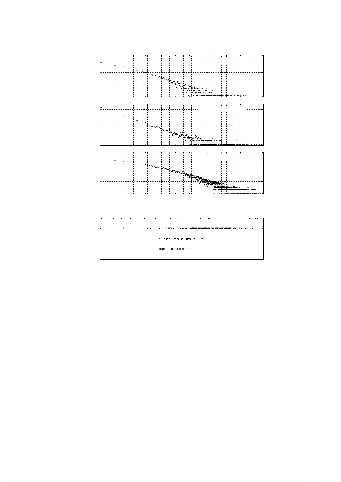
1 Statistical T opic Models f or Multi-Label Document Classiﬁcation Timoth y Rubin T RU B I N @ U C I . E D U Department of Cognitive Sciences University of California, Irvine Irvine, CA 92697, USA America Chambers A H O L L OWA @ U C I . E D U Department of Computer Science University of California Irvine, CA 92697, USA Padhraic Smyth S M Y T H @ I C S . U C I . E D U Department of Computer Science University of California Irvine, CA 92697, USA Mark Steyvers M A R K . S T E Y V E R S @ U C I . E D U Department of Cognitive Sciences University of California, Irvine Irvine, CA 92697, USA Abstract Machine learning approaches to multi-label document classiﬁcation have to date largely relied on discriminative modeling techniques such as support vector machines. A dra wback of these approaches is that performance rapidly drops off as the total number of labels and the number of labels per document increase. This problem is ampliﬁed when the label frequencies exhibit the type of highly ske wed distributions that are often observed in real-world datasets. In this paper we in vestigate a class of generativ e statistical topic models for multi-label documents that associate individual word tokens with different labels. W e in vestigate the adv antages of this approach relative to discriminativ e models, particularly with respect to classiﬁcation problems inv olving large numbers of relatively rare labels. W e compare the performance of generative and discriminativ e approaches on document labeling tasks ranging from datasets with several thousand labels to datasets with tens of labels. The experimental results indicate that probabilistic generative models can achieve competitive multi-label classiﬁcation performance compared to discriminative methods, and ha ve advantages for datasets with man y labels and ske wed label frequencies. Keyw ords: T opic Models; LD A; Multi-Label Classiﬁcation; Document Modeling; T e xt Classiﬁcation; Graphical Models; Probabilistic Generativ e Models; Dependency-LD A 1. Introduction The past decade has seen a wide variety of papers published on multi-label document classiﬁcation, in which each document can be assigned to one or more classes. In this introductory section we begin by discussing the limitations of existing multi-label document classiﬁcation methods when applied to datasets with statistical properties common to real-w orld datasets, such as the presence of large numbers of labels with po wer-law-like frequency statistics. W e then motiv ate the use of generative probabilistic models in this context. In particular , we illustrate ho w these models can be advantageous in the conte xt of large-scale multi-label corpora, through (1) explicitly assigning individual words to speciﬁc labels within each document—rather than assuming that all of the words within a document are relev ant to each of its labels, and (2) jointly modeling all labels within a corpus simultaneously , which lends itself well to the task of accounting for the dependencies between these labels. 1.1 Background and Moti vation Much of the prior work on multi-label document classiﬁcation uses data sets in which there are relatively few labels, and many training instances for each label. In many cases, the datasets are constructed such that they contain few , if an y , infrequent labels. For e xample, in the commonly used RCV1-v2 corpus (Le wis et al., 2004), the dataset was carefully constructed to hav e approximately 100 labels, with most labels occurring in a relativ ely large number of documents. 2 Power-Law Datasets 10 2 10 3 E UR -Le x C o rp us QUENCY X 10 0 10 1 10 2 10 3 10 0 10 1 B ELS WITH FRE 10 1 10 2 10 3 NY T Ann o ta te d Co r p u s # UNIQUE LA B 2 10 3 O HS U M E D C o rp us 10 0 10 1 10 2 10 3 10 0 10 0 10 1 10 2 10 3 10 0 10 1 10 2 Non Power-Law Datasets # DOCUMENTS PER LABEL 10 10 10 10 RCV1 - V2 RCV1 V2 Y! Health Y! Arts # DOCUMENTS PER LABEL 10 0 10 1 10 2 10 3 10 4 10 5 10 6 F ig. 1: T op : The number of unique labels (y-axis) that hav e K training documents (x-axis) for three large-scale multi-label datasets. Both axes are shown on a log-scale. The power-la w-like relationship is evident from the near linear trend (in log-space) of this relationship. Bottom : The number of training documents(x-axis) for each unique label in three common (non-power-la w) benchmark datasets. Since there are no label-frequencies at which there are more than one unique label in any of the datasets, if these plots were sho wn using the log-log scale used in the plots above, all points would fall along the y value corresponding to 10 0 . Note that the scaling of the x-axis is not equiv alent for the power -law and non po wer-law plots (this is necessary due to the high upper-bound of label-frequencies on the RCV1-V2 dataset). In other cases researchers hav e typically restricted the problem by only considering a subset of the full dataset. As an example, a popular source of experimental data has been the Y ahoo! directory structure, which utilizes a multi-labeling classiﬁcation system. The true Y ahoo! directory structure contains thousands of labels and is a very difﬁcult classiﬁcation problem that traditional classiﬁcation methods fail to adequately handle (Liu et al., 2005). Howe ver , the majority of multi-label research conducted using the Y ahoo! directory data has been performed on the set of 11 sub-directory datasets constructed by Ueda and Saito (2002). Each of these datasets consists of only the second-lev el categories from a single top-level Y ahoo! directory , leaving only about 20-30 labels in each of the classiﬁcation tasks. Furthermore, many of the publications (e.g., Ueda and Saito, 2002; Ji et al., 2008) that use the Y ahoo! subdirectory datasets have remov ed the infrequent labels from the ev aluation data, leaving between 14 and 23 unique labels per dataset. Similarly , experiments with the OHSUMED MeSH terms (Hersh et al., 1994) 3 are typically performed on a small subdirectory that contains only 119 out of over 22,000 possible labels (for a discussion, see Rak et al. (2005)). In contrast to the datasets typically utilized in research, multilabel corpora in the real world can contain thousands or tens of thousands of labels, and the label frequencies in these datasets tend to hav e highly skewed frequency-distrib utions with power -law statistics (Y ang et al., 2003; Liu et al., 2005; Dekel and Shamir, 2010). Figure 1 illustrates this point for three large real-world corpora—each containing thousands of unique labels—by plotting the number of labels within each corpus as a function of label-frequency . F or each corpus, the total number of labels is plotted as a function of label-frequenc y on a log-log scale (i.e., more precisely , number of unique labels [y-axis] that have been assigned to k documents in the corpus is plotted as a function of k [x-axis]). Of note is the power -law like distrib ution of label frequencies for each corpus, in which the v ast majority of labels are associated with very few documents, and there are relativ ely fe w labels that are assigned to a large number of documents. For example, roughly one thousand labels are only assigned to a single document in each corpus, and the median label- frequencies are 3, 6, and 12 for the NYT , EUR-Lex, and OHSUMED datasets, respecti vely . This stands in stark contrast to the widely-used Y ahoo! Arts , Y ahoo! Health and RCV1-v2 datasets (for example), which are shown at the bottom of Figure 1. In these corpora, there are hardly any labels that occur in fewer than 100 documents, and the median label-frequencies are 530, 500, and 7,410 respecti vely (see Section 4 for further details and discussion). T o summarize, these popular benchmark datasets are drastically dif ferent from lar ge-scale real-world corpora not only in terms of the number of unique labels they contain, but also with respect to the distribution of label-frequencies, and in particular the number of rare labels. The mismatch between real-world and experimental datasets has been discussed pre viously in the literature, notably by Liu et al. (2005) who observ ed that although popular multi-label techniques—such as “one-vs-all” binary classiﬁcation (e.g. Allwein et al., 2001; Rifkin and Klautau, 2004)—can perform well on datasets with relativ ely few labels, performance drops off dramatically on real world datasets that contain many labels and skewed label frequency distributions. In addition, Y ang (2001) illustrated that discriminative methods which achiev e good performance on standard datasets do relativ ely poorly on larger datasets such as the full OHSUMED dataset. The obvious reason for this is that discriminative binary classiﬁers have difﬁculty learning models for labels with very few positi vely labeled documents. As stated by Liu et al. (2005), in the context of support vector machine (SVM) classiﬁers: In terms of effecti veness, neither ﬂat nor hierarchical SVMs can fulﬁll the needs of classiﬁcation of very large-scale taxonomies. The skewed distribution of the Y ahoo! Directory and other large taxonomies with many e xtremely rare categories makes the classiﬁcation performance of SVMs unacceptable. More sub- stantial inv estigation is thus needed to improv e SVMs and other statistical methods for very large-scale applications. A second critical dif ference between large scale multi-label corpora and traditional benchmark datasets relates to the number of labels that are assigned to each document. Figure 2 compares the distributions of the number of labels per document for the same corpora shown in Figure 1. The median number of labels per document for the real world, power-la w style datasets are 6, 5, and 12 for EUR-Lex, NYT and OHSUMED, respectiv ely . These numbers are signiﬁcantly larger than those in the typical datasets used in multi-label classiﬁcation e xperiments. For example, among the three benchmark datasets sho wn, the RCV1-v2 dataset has a median of 3 labels per document, and the Y ahoo! Arts and Health datasets each ha ve a median of only 1 label per document. These differences can signiﬁcantly impact the performance of a classiﬁer . As the number of labels per document increases, it becomes more dif ﬁcult for a discriminativ e algorithm to distinguish which words are discriminativ e for a particular label. This problem is further compounded when there is little training data per label. For the purposes of illustration, consider the following extreme case: suppose that we are training a binary classiﬁer for a label, c 1 , that has only been assigned to one document, d . Furthermore, assume that two additional labels, c 2 and c 3 , have been assigned to document d , and that these labels occur in a relativ ely large number of documents. Since document d is the only positive training example for label c 1 , an independent binary classiﬁer trained on c 1 will learn a discriminant function that emphasizes not only words from document d that are relev ant to label c 1 , but also words that are relev ant to labels c 2 and c 3 , since the classiﬁer has no way of “knowing” which words are relev ant to these other labels. In other words, when training an independent binary classiﬁer for label c 1 , each additional label that co-occurs with c 1 will introduce additional confounding features for the classiﬁer , thereby reducing the quality of the classiﬁer . 4 60 0 0 80 00 EU RLex P o w er- Law Da tase ts 40 00 50 00 Ya hoo! A rts No n Power - Law Da tase t s T S 0 20 00 40 00 60 00 0 10 00 20 00 30 00 20 00 30 00 40 00 50 00 Ya hoo! Hea lth 40 00 60 00 80 00 NY T Corp us O F DOC UMEN T 0 10 00 20 00 20 000 OS 40 0000 C1 2 0 20 00 NU MBER O 0 10 000 O H S UME D 0 20 0000 R C V 1 -V 2 0 5 10 15 20 25 0 N U MBE R O F LAB EL S AS SIGN ED T O DO CU M EN T 0 5 10 15 20 25 0 N U MBE R O F LAB ELS AS SIG N ED T O DO CU ME N T F ig. 2: Number of documents (y-axis) that have L labels (x-axis). The version of the NYT Annotated Corpus used in our experiments contains documents with 3 or more labels, hence the cutoff at 3. Note howe ver that in the above example it should be relatively easy to learn which features are relev ant to the labels c 2 and c 3 , since these labels occur in a large number of documents. Thus, we should be able to leverage this information to improv e our classiﬁer for c 1 by removing the features in d which we kno w to be relev ant to these confounding labels. One possible approach to address this problem is to learn which individual word tokens within a document are likely to be associated with each label. If we could then use this information to identify which words within d are likely to be related to c 2 and c 3 , we could “explain away” these words, and then use the remaining words for the purposes of learning a model for c 1 . Note that for this purpose it is useful to (1) remo ve the assumption of label-wise independence, and (2) learn the models for all of the labels simultaneously , since learning which words within a document are irrele vant to a particular label is a ke y part of learning which words are relev ant to the label. 1.2 A Generative Modeling A pproach In a generative approach to document classiﬁcation, one learns a model for the distribution of the words given each label, i.e., a model for P ( w | c ) , 1 ≤ c ≤ C , where w is the set of words in a document, and constructs a discriminant function for the label via Bayes rule. In standard supervised learning, with one label per document, these C distrib utions are typically learned independently . W ith multi-label data, the distrib utions should instead be learned simultaneously since we cannot separate the training data into C groups by label. A useful approach in this context is a model known as latent Dirichlet allocation (LDA) (Blei et al., 2003), which we will also refer to as topic modeling, which models the words in a document as being generated by a mix- ture of topics, i.e., P ( w | d ) = P c P ( w | c ) P ( c | d ) , where P ( w | d ) is the marginal probability of word w in document d , P ( w | c ) is the probability of word w being generated given label c , and P ( c | d ) is the relative probability of each of the c labels associated with document d . LD A has primarily been vie wed as an unsupervised learning algorithm, but can also be used in a supervised conte xt (e.g., Blei and McAuliffe, 2008; Mimno and McCallum, 2008; Ramage et al., 2009). Using a supervised v ersion of LD A it is possible to learn both the w ord-label distrib utions P ( w | c ) and the document-label weights P ( c | d ) given a training corpus with multi-label data. What is particularly relev ant is that this approach (1) models the assignment of labels at the word-lev el, rather than at the document le vel as in discriminativ e models, and (2) learns a model for all labels at the same time, rather than treating each label independently . In particular, for the document d in our earlier e xample that was assigned the set of labels { c 1 , c 2 , c 3 } , the model can explain away words that belong to labels c 2 and c 3 —i.e., words that have high probability P ( w | c ) under these labels. Since c 2 and c 3 are frequent labels, it will be relativ ely easy to learn which features are relevant to these labels, since the confounding features introduced by co-occurring labels in a multi-label scheme will tend to cancel out o ver many documents. The remaining words that cannot be explained 5 well by c 2 or c 3 will be assigned to label c 1 , and the model will learn to associate such words with this label and not associate with c 1 the words that are more likely to belong to labels c 2 and c 3 . This general intuition is the basis for our approach in this paper . Speciﬁcally , we in vestigate supervised v ersions of topic models (LD A) as a general framew ork for multi-label document classiﬁcation. In particular , the topic modeling approach allows for the type of “explaining away” ef fect at the word le vel that we hypothesize should be particularly helpful for the types of rare labels that pose challenges to purely discriminativ e methods. Document  Labels Label  Freq. SVM   (weight) LDA  (prob.) A NTITRUST  A CTIONS  AND  L AWS 19 nintendo  nintendo  S UITS  AND  L ITIGATION 67 mcgowan  games  V IDEO  G AMES  1 futuristic  software  compatible  video  illusion  system  shrewd  game  inception  chip  truthful  control  profiles  market  billionayear  home  suing  computer  infringement  shortage  architecture  say  handheld  buy  tantamount  demand  payoff  developer  NY  Times  Article Models  for  V IDEO  G AMES Document  Excerpt A flurry of lawsuits, started by a small American software developer, now surrounds the Nintendo Entertainment System, the best- selling toy in the United States last year...Atari Games argues that Nintendo's high degree of control is tantamount to monopoly, and is suing Nintendo for antitrust violations... F ig. 3: High-weight and high probability words for the label V I D E O G A M E S learned by an SVM classiﬁer and an LDA model (respec- tiv ely) from the a set of New Y ork Times articles, in which the label V I D E O G A M E S only appeared once (text from the article is shown on the left). Figure 3 illustrates the advantages an LD A-based approach has in terms of learning rare labels. On the left is the partial text of a news article, taken from the New Y ork Times, along with three human-assigned labels: A N T I T R U S T AC T I O N S A N D L AW S and S U I T S A N D L I T I G AT I O N (which both occur in multiple other documents) and V I D E O G A M E S (for which this document is the only positi ve example in the training data). On the right are the words with the highest weights from a binary SVM classiﬁer trained on the label V I D E O G A M E S . Beside this column are the highest probability words learned by an LD A-based model (described in more detail later in the paper). The words learned by the SVM classiﬁer are quite noisy , containing a mixture of words relev ant to the other two labels (e.g., suing , infringement , etc...), as well as rare words that are peculiar to the speciﬁc document rather than being relev ant features for any of the labels (e.g., futuristic , illusion , etc...). These words do not match our intuition of words that would be discriminativ e for the concept V I D E O G A M E S . Furthermore, as we will see later in the experimental results section, SVM classiﬁers trained on rare labels in this type of multi-label problem do not predict well on new test documents. While the set of words learned by LDA model is still somewhat noisy , it is nonetheless clear the model has done a better job in determining which words are relev ant to the label V I D E O G A M E S , and which of the words should be associated with the other two labels (e.g., there are no words with high probability that directly relate to lawsuits). The model beneﬁts from not assuming independence between the labels, as with binary SVMs, as well as from the “explaining a way” ef fect. Thus far we hav e focused our discussion on the issue of learning appropriate models for labels during train- ing. An additional issue that arises as the number of total labels (as well as the number of labels per document) increases, is the importance of accounting for higher-order dependencies between labels at prediction time (i.e., when classifying a ne w document). For example, suppose that we are predicting which labels should be assigned to a test-document that contains the word ster oids . In a large-scale dataset like the NYT corpus, this word is a high-probability feature among many different labels, such as M E D I C I N E A N D H E A LT H , B A S E B A L L , and B L AC K M A R K E T S . The ambiguity in the assignment of this word to a speciﬁc label can often be resolv ed if we account for the other labels within the document; e.g., the word ster oids is lik ely to be related to the label B A S E B A L L giv en that 6 the label S U S P E N S I O N S , D I S M I S S A L S A N D R E S I G N A T I O N S is also assigned to the document, whereas it is more likely to be related to M E D I C I N E A N D H E A LT H given the presence of the label C A N C E R . Giv en this motiv ation, an additional beneﬁcial feature of the topic model—and probabilistic methods in general— is that it is relativ ely straightforward to model the label dependencies that are present in the training data (a feature that we will elaborate on later in the paper). Modeling label dependencies is widely acknowledged to be impor- tant for accurate classiﬁcation in multi-label problems, yet has been problematic in the past for datasets with large numbers of labels, as summarized in Read et al. (2009): The consensus vie w in the literature is that it is crucial to take into account label correlations during the classiﬁcation process ..... Ho wever as the size of the multi-label datasets grows, most methods struggle with the exponential growth in the number of possible correlations. Consequently these methods are able to be more accurate on small datasets, but are not as applicable to lar ger datasets. Thus, the ability of probabilistic models to account for label dependencies is a strong motiv ation for considering these types of approaches in large-scale multi-label classiﬁcation settings. 1.3 Contributions and Outline In the context of the discussion above, this paper inv estigates the application of statistical topic modeling to the task of multi-label document classiﬁcation, with an emphasis on corpora with lar ge numbers of labels. W e consider a set of three models based on the LD A framew ork. The ﬁrst model, Flat-LDA , has been employed previously in various forms. Additionally , we present two new models: Prior-LD A , which introduces a no vel approach to account for variations in label frequencies, and Dependency-LDA , which extends this approach to account for the dependencies between the labels. W e compare these three topic models to two variants of a popular discriminati ve approach (one-vs-all binary SVMs) on ﬁv e datasets with widely contrasting statistics. W e ev aluate the performance of these models on a v ariety of predictions tasks. Speciﬁcally , we consider (1) document-based rankings (rank all labels according to their rele vance to a test document) and binary predictions (make a strict yes/no classiﬁcation about each label for a gi ven document), and (2) label-based rankings (rank all documents according to their relev ance to a label) and binary predictions (make a strict yes/no classiﬁcation about each document for a giv en label). The speciﬁc contributions of this paper are as follo ws: – W e describe two novel generative models for multi-label document classiﬁcation, including one (Dependency- LD A) which signiﬁcantly impro ves performance over simpler models by accounting for label dependencies, and is highly competitiv e with popular discriminati ve approaches on large-scale datasets. – W e report extensi ve e xperimental results on two multi-label corpora with lar ge numbers of labels as well as three smaller benchmark datasets, comparing the proposed generati ve models with discriminative SVMs. T o our knowledge this is the ﬁrst empirical study comparing generative and discriminativ e models on large-scale multi-label problems. – W e demonstrate that LD A-based models—in particular the Dependency-LD A model—can be highly competi- tiv e with, or better than, SVMs on large-scale datasets with po wer-law like statistics. – For document-based predictions, we show that Dependency-LD A has a clear advantage over SVMs on lar ge- scale datasets, and is competitiv e with SVMs on the smaller , benchmark datasets. – For label-based predictions, we demonstrate that Dependency-LD A generally outperforms SVMs on large- scale datasets. W e furthermore show that there is a clear performance adv antage for the LDA-based methods on rare labels (e.g., labels with fewer than 10 training documents). The remainder of the paper is organized as follo ws. W e begin by describing how standard unsupervised LDA can be adapted to handle multi-labeled text documents, and describe our extensions that incorporate label frequencies and label dependencies. W e then describe how inference is performed with these models, both for learning the model from training data and for making predictions on new test documents. An extensi ve set of experimental results are then presented on a wide range of prediction tasks on ﬁv e multi-label corpora. W e conclude the paper with a discussion of the relati ve merits of the LD A-based approaches vs. SVM-based approaches, particularly in the context of both the dataset statistics and prediction tasks being considered. 7 2. Related W ork A number of approaches ha ve been proposed for adapting the unsupervised LD A model to the case of supervised learning—such as the Supervised T opic Model (Blei and McAuliffe, 2008), Semi-LD A (W ang et al., 2007), Dis- cLD A (Lacoste-Julien et al., 2008), and MedLD A (Zhu et al., 2009) —howe ver , these adaptations are designed for single label classiﬁcation or regression, and are not directly applicable to multilabel classiﬁcation. A more recent approach proposed by Ramage et al. (2009)—Labeled-LD A (L-LD A)—was designed specif- ically for multi-label settings. In L-LD A, the training of the LD A model is adapted to account for multi-labeled corpora by putting “topics” in 1-1 correspondence with labels and then restricting the sampling of topics for each document to the set of labels that were assigned to the document, in a manner similar to the Author-Model described by Rosen-Zvi et al. (2004) (where the set of authors for each document in the Author Model is now replaced by the set of labels in L-LDA). The primary focus of Ramage et al. (2009) was to illustrate that L-LD A has certain qualitativ e adv antages over discriminati ve methods (e.g., the ability to label indi vidual words, as well as pro viding interpretable snippets for document summarization). Their classiﬁcation results indicate that under certain condi- tions LDA-based models may be able to achiev e competitive performance with discriminativ e approaches such as SVMs. Our work dif fers from that of Ramage et al. (2009) in two signiﬁcant aspects. Firstly , we propose a more ﬂexible set of LD A models for multi-label classiﬁcation—including one model that takes into account prior label frequencies, and one that can additionally account for label dependencies—which lead to signiﬁcant improv e- ments in classiﬁcation performance. The L-LD A model can be viewed as a special case of these models. Secondly , we conduct a much lar ger range and more systematic set of experiments, including in particular datasets with large numbers of labels with ske wed frequency-distributions, and show that generativ e models do particularly well in this regime compared to discriminative methods. In contrast, Ramage et al. (2009) compared their L-LD A ap- proach with discriminati ve models only on relativ ely small datasets (primarily on the Y ahoo! sub-directory datasets discussed in the introduction). Our work (as well as the Author Model and L-LD A model) can be seen as building on earlier ideas from the literature in probabilistic modeling for multilabel classiﬁcation. McCallum (1999) and Ueda and Saito (2002) in vestigated mixture models similar to L-LD A, where each document is composed of a number of word distribu- tions associated with document labels. These papers can be viewed as early forerunners of the more general LD A framew orks we propose in this paper . More recently Ghamrawi and McCallum (2005) demonstrated that the probabilistic framew ork of conditional random ﬁelds sho wed promise for multilabel classiﬁcation, compared to discriminati ve classiﬁers, as the number of labels within test documents increased. In follow-up work on these models, Druck et al. (2007) illustrated that this approach has the further beneﬁt of being able to naturally incorporate unlabeled data for semi-supervised learning. A drawback of the CRF approach is scalability , particularly when accounting for label dependencies. Exact inference “is tractable only for about 3-12 [labels]” (Ghamrawi and McCallum, 2005). Alternativ es to exact inference considered in Ghamrawi and McCallum (2005) include a “supported inference” method which learns only to classify the label combinations that occur in the training set, and a binary-pruning method that employs an intelligent pruning method which ignores dependencies between all but the most commonly observ ed pairs of labels. Although this method may improve upon approaches that ignore dependencies when restricted to datasets with fe w labels and man y examples (such as traditional benchmark datasets), it seems unlikely that an y such methods will be able to properly account for dependencies in datasets with power -law frequency statistics (since nearly all dependencies in these datasets are between labels which hav e very sparse training data). Zhang and Zhang (2010) present a hybrid generativ e-discriminati ve approach to multi-label classiﬁcation. They ﬁrst learn a Bayesian network structure that represents the independencies between labels. They then learn a dis- criminativ e classiﬁer for each label in the order speciﬁed by the Bayesian netw ork where the classiﬁer for label c takes as features not only the words in the document but also the output of the classiﬁers for each of the labels in the parent set of c (i.e. the parent set speciﬁed by the Bayesian network). Howe ver , they apply their model to only small-scale datasets (the largest ha ving 158 labels). In terms of discriminative approaches to multi-label classiﬁcation, there is a lar ge body of prior work, which has been well-summarized else where in the literature (e.g., see Tsoumakas and Katakis, 2007; Tsoumakas et al., 2009). Most discriminative approaches to multi-label classiﬁcation hav e employed some v ariant of the “binary problem-transformation” technique, in which the multi-label classiﬁcation problem is transformed into a set of 8 θ ' γ c β c z'  ' β c c  ' α ' c M M T  c α  α ' c α   z β w θ z β w θ α z β w θ D C z w  N C z w  D D C z w  N N D D D Dependency ‐ LD A Prior ‐ LD A Flat ‐ LD A F ig. 4: Graphical models for multi-label documents. The observed data for each document d are a set of words w ( d ) and labels c ( d ) . Left : In Flat-LD A, no generativ e assumptions are made re garding ho w labels are generated; labels for each document are assumed to be giv en. Center : The Prior-LD A model assumes that the label-tokens c ( d ) for each document are generated by sampling from a corpus- wide multinomial distrib ution o ver label-types φ 0 , which captures the relati ve frequencies of different label-types across the corpus. Right : The Dependency-LD A model assumes that the label-tokens for each document are sampled from a set of T corpus-wide topics — where each “topic” t corresponds to a multinomial distribution over label-types φ 0 t —according to a document-speciﬁc distribution θ 0 d over these topics. binary-classiﬁcation problems, each of which can then be solv ed using a suitable binary classiﬁer (Rifkin and Klautau, 2004; Tsoumakas and Katakis, 2007; Tsoumakas et al., 2009; Read et al., 2009). The most commonly employed method in the literature is the “one-vs-all” transformation, in which C independent binary classiﬁers are trained—one classiﬁer for each label. These binary classiﬁcation tasks are then handled using discriminativ e classiﬁers, most notably SVMs, but also via other methods such as perceptrons, naive Bayes, and kNN classiﬁers. As our baseline discriminati ve method in this paper, we use the “one-vs-all” approach with SVMs as the binary classiﬁer , since this is the most commonly used discriminativ e approach in the current multi-label classiﬁcation literature, and has been defended in the literature in the f ace of an increasing number of proposed alternati ve methods (e.g., see Rifkin and Klautau, 2004). W e note also that there is a prior thread of work on discriminativ e approaches that can handle label-dependencies. F or example, another problem-transformation technique known as the “Label Powerset” method (Tsoumakas et al., 2009; Read et al., 2009) builds a binary classiﬁer for each distinct subset of label-combinations that exist in the training data—howe ver , these approaches tend not to scale well with large label sets due to combinatorial ef fects (Read et al., 2009). 3. T opic Models f or Multilabel Documents In this section, we describe three models (depicted in Figure 4 using graphical model notation) that e xtend the tech- niques of topic modeling to multi-label document classiﬁcation. Before pro viding the details for each model, we ﬁrst brieﬂy introduce the notation that will be used to describe these topic models within the multi-label inference setting, as well as provide a high-le vel description of the relationships between the three models. The general setup of the inference task for the multi-label topic models we describe is as follo ws: the observ ed data for each document d ∈ { 1 , . . . , D } are a set of words w ( d ) and labels c ( d ) . F or all models, each label- type c ∈ { 1 , . . . , C } is modeled as a multinomial distribution φ c ov er words. Each document d is modeled as a 9 multinomial distrib ution θ d ov er the document’ s observed label-types. W ords for document d are generated by ﬁrst sampling a label-type z from θ d , and then sampling a word-token w from φ z . The three models that we present differ with respect to ho w they model the generativ e process for labels. The ﬁrst model we describe is a straightforward extension of LD A to labeled documents, which we will refer to as Flat-LD A, where the labels are treated as given; this model makes no generative assumptions regarding how labels c ( d ) are generated for a document. W e then describe an extension to the Flat-LD A model—Prior-LD A—that incorporates a generativ e process for the labels themselves via a single corpus-wide multinomial distribution over all the label-types in the corpus. This assumption of Prior-LD A is very useful for making predictions when the label-frequencies are highly non-uniform. Lastly , we describe Dependency-LD A, which is a hierarchical extension to the previous two models that captures the dependencies between the labels by modeling the generative process for labels via a topic model; in Dependenc y-LD A, label-tokens for each document d are sampled from a set of T corpus-wide topics, according to a document-speciﬁc distrib ution θ 0 d ov er the topics. W e note that the Flat-LDA and Prior-LD A models can be viewed as special cases of the Dependency-LD A model. In particular , the Prior-LD A model is equiv alent Dependency-LD A if we set the number of topics T = 1 . 3.1 Flat-LD A The latent Dirichlet allocation (LDA) model, also referred to as the topic model, is an unsupervised learning tech- nique for extracting thematic information, called topics, from a corpus. LDA represents topics as multinomial dis- tributions o ver the W unique word-types in the corpus and represents documents as a mixture of topics. Flat-LDA is a straightforward extension of the LDA model to labeled documents. The set of LD A topics is substituted with the set of unique labels observed in the corpus. Additionally , each document’ s distribution ov er topics is restricted to the set of observed labels for that document. More formally , let C be the number of unique labels in the corpus. Each label c is represented by a W - dimensional multinomial distribution φ c ov er the v ocabulary . For document d , we observe both the words in the document w ( d ) as well as the document labels c ( d ) . The generativ e process for Flat-LD A is sho wn below . Each document is associated with a multinomial distribution θ d ov er its set of labels. The random vector θ d is sampled from a symmetric Dirichlet distrib ution with hyper -parameter α and dimension equal to the number of labels | c ( d ) | . Giv en the distribution o ver topics θ d , generating the words in the document follo ws the same process as LD A: 1. For each label c ∈ { 1 , . . . , C } , sample a distribution over w ord-types φ c ∼ Dirichlet( ·| β ) 2. For each document d ∈ { 1 , . . . , D } (a) Sample a distribution over its observ ed labels θ d ∼ Dirichlet( ·| α ) (b) For each word i ∈ { 1 , . . . , N W d } i. Sample a label z ( d ) i ∼ Multinomial ( θ d ) ii. Sample a word w ( d ) i ∼ Multinomial ( φ c ) from the label c = z ( d ) i Note that this model assigns each word token within a document to just a single label—speciﬁcally to one of the labels that w as assigned to the document. The model is depicted using graphical model notation in the left panel of Figure 4. Due to the similarity between the Flat-LD A model presented here, and both the Author-Model from Rosen-Zvi et al. (2004) and the L-LD A model from Ramage et al. (2009), it is important to note precisely the relationships between these models. The Author-Model is conditioned on the set of authors in a document (and a “topic” is learned for each author in the corpus), whereas L-LD A and Flat-LD A are conditioned on the set of labels assigned to a document (and a “topic” is learned for each label in the corpus). L-LD A and Flat-LD A are in practice equiv alent models, but employ different generativ e descriptions. Speciﬁcally , L-LDA models the generative process for each label in a document as a Bernoulli variable (where the parameter of the Bernoulli distribution is label-dependent). Howe ver , during training, estimating the Bernoulli parameters is independent from learning the assignment of words to labels (i.e. the z v ariables). Thus, during training both L-LD A and Flat-LDA reduce to standard LD A with an additional restriction that words can only be assigned to the observed labels in the document. Similarly , when performing inference for unlabeled documents (i.e. at test time), Ramage et al. (2009) assume that L-LD A reduces to standard LDA. In this way , both Flat-LD A and L-LDA are in practice equi valent despite L-LD A including a 10 generativ e process for labels 1 . Due to the mismatch between the generative description of L-LD A and how it is employed in practice, we ﬁnd it pedagogically useful to distinguish between the models presented here and L-LD A 3.2 Prior -LD A An obvious issue with Flat-LD A is that it does not account for differences in the relative frequencies of the labels within a corpus. This is not a problem during training, because all labels are observed for training documents. Howe ver , for the purpose of prediction (labeling ne w documents at test-time), accounting for the prior probabilities of each label becomes important, particularly when there are dramatic dif ferences in the frequencies of labels in a corpus (as is the case with power -law datasets, as well as with many traditional datasets, such as RCV1-V2). In this section we present Prior-LD A, which extends Flat-LDA by incorporating a generativ e process for labels that accounts for differences in the observed frequencies of different label types. This is achieved using a two- stage generative process for each document, in which we ﬁrst sample a set of observed labels from a corpus-wide multinomial distribution, and then gi ven these labels, generate the words in the document. Let φ 0 be a corpus-wide multinomial distribution ov er labels (reﬂecting, for example, a po wer-law distrib ution of label frequencies). For document d , we draw M d samples from φ 0 . Each sample can be thought of as a single vote for a particular label. W e replace α ( d ) , the symmetric Dirichlet prior with hyperparameter α , with a C -dimensional vector α 0 ( d ) where the i th component is proportional to the total number of times label i was sampled from φ 0 . Formally , the vector α 0 ( d ) is deﬁned to be: α 0 ( d ) =  η ∗ N d, 1 M d + α , η ∗ N d, 2 M d + α , . . . , η ∗ N d,C M d + α  (1) where N d,i is the number of times label i was sampled from φ 0 . In other words, α 0 ( d ) is a scaled, smoothed, normalized vector of label counts 2 . The hyper -parameter η speciﬁes the total weight contributed by the observed labels c ( d ) and the hyper-parameter α is an additional smoothing parameter that contributes a ﬂat pseudocount to each label. W e deﬁne the document’ s label set c ( d ) to be the set of labels with a non-zero component in α 0 ( d ) . T o make this model fully generati ve, we place a symmetric Dirichlet prior on φ 0 . Consider , for example, three labels { c 1 , c 2 , c 3 } with frequencies φ 0 = { 0 . 5 , 0 . 3 , 0 . 2 } in the corpus. For doc- ument d , we draw M d samples from φ 0 . Assume M d = 5 and the set { c 1 , c 2 , c 1 , c 1 , c 1 } was sampled. Then the hyper-parameter α 0 ( d ) would be: α 0 ( d ) = h η ∗ 4 5 + α , η ∗ 1 5 + α , η ∗ 0 5 + α i If hyperparameter α = 0 , then α 0 ( d ) has only two non-zero components (because the last component equals zero) and c ( d ) = { c 1 , c 2 } . In this case, the multinomial vector θ d drawn from Dirichlet  α 0 ( d )  will alw ays ha ve zero count for the third label (i.e. label c 3 will hav e probability zero in the document). If α > 0 , then c ( d ) = { c 1 , c 2 , c 3 } and label c 3 will have non-zero probability in the document. As M d goes to inﬁnity , α 0 ( d ) approaches the vector η φ 0 + α . The multinomial distrib ution may seem like an unnatural choice for a label-generating distrib ution since the observed labels in a document are most naturally represented using binary variables rather than counts. W e exper- imented with alternati ve parameterizations such as a multiv ariate Bernoulli distrib ution. Ho wever , this introduced problems during both training and testing. As noted by Schneider (2004) in relation to modeling document wor ds (rather than labels), the multiv ariate Bernoulli distribution tends to overweight negati ve evidence (i.e. the absence of a word in a document) during training, due to the sparsity of the word-document matrix. This problem is com- pounded when modeling document labels because there are considerably fewer labels in a document than w ords. Furthermore, at test time when the document labels are unobserved, a Bernoulli model will conv erge more slowly since the probability of turning on a label in a document is higher than the probability of turning of f a label in a 1. Due to equiv alence of Flat-LD A and L-LDA in practice, the experimental results we present for Flat-LDA are equivalent to what would be expected for L-LD A 2. In the training data, we set M d equal to the number of observed labels in document d and N d,i equal to 0 or 1 depending upon whether the label is present in the document. 11 document (this is due to the fact that a label can only be turned off after all words assigned to that label hav e been assigned elsewhere) 3 . The generativ e process for the Prior-LD A model is: 1. Sample a multinomial distribution over labels φ 0 ∼ Dirichlet( ·| β C ) 2. For each label c ∈ { 1 , . . . , C } , sample a distribution over w ord-types φ c ∼ Dirichlet( ·| β W ) 3. For each document d ∈ { 1 , . . . , D } : (a) Sample M d label tokens c ( d ) j ∼ Multinomial ( φ 0 ) , 1 ≤ j ≤ M d (b) Compute the Dirichlet prior α 0 ( d ) for document d according to Equation 1 (c) Sample a distribution over labels θ d ∼ Dirichlet  ·| α 0 ( d )  (d) For each word i ∈ { 1 , . . . , N W d } i. Sample a label z ( d ) i ∼ Multinomial ( θ d ) ii. Sample a word w ( d ) i ∼ Multinomial ( φ c ) from the label c = z ( d ) i This model is depicted using graphical model notation in the center panel of Figure 4. 3.3 Dependency-LD A Prior-LD A accounts for the prior label frequencies observed in the training set, but it does not account for the dependencies between the labels, which is crucial when making predictions for new documents. In this section, we present Dependenc y-LD A, which extends Prior-LD A by incorporating another topic model to capture the de- pendencies between labels. The labels are generated via a topic model where each “topic” is a distribution ov er labels. Dependency-LD A is an extension of Prior-LD A in which there are T corpus-wide probability distributions ov er labels, which capture the dependencies between the labels, rather than a single corpus-wide distribution that merely reﬂects relativ e label frequencies. W e note that several models that represent or induce topic dependencies hav e been in vestigated in the past for unsupervised topic modeling (e.g., Blei and Lafferty (2005); T eh et al. (2004); Mimno et al. (2007); Blei et al. (2010)). Although these models are related to varying degrees to the Dependency- LD A model, as unsupervised models they are not directly applicable to document classiﬁcation. Formally , let T be the total number of topics where each topic t is a multinomial distribution over labels denoted φ 0 t . Generating a set of labels for a document is analogous to generating a set of words in LD A. W e ﬁrst sample a distribution over topics θ 0 d . T o generate a single label we sample a topic z 0 from θ 0 d and then sample a label from the topic φ 0 z 0 . W e repeat this process M d times. As in Prior-LD A, we compute the hyper-parameter v ector α 0 ( d ) according to Equation 1 and deﬁne the label set c ( d ) as the set of labels with a non-zero component. Giv en the set of labels c ( d ) , generating the words in the document follo ws the same process as Prior-LD A. 1. For each topic t ∈ { 1 , . . . , T } , sample a distribution o ver labels, φ 0 t ∼ Dirichlet( β C ) 2. For each label c ∈ { 1 , . . . , C } , sample a distribution over w ords, φ c ∼ Dirichlet( β W ) 3. For each document d ∈ { 1 , . . . , D } : (a) Sample a distribution over topics θ 0 d ∼ Dirichlet( γ ) (b) For each label j ∈ { 1 , . . . , M d } i. Sample a topic z 0 ( d ) j ∼ Multinomial ( θ 0 d ) ii. Sample a label c ( d ) j ∼ Multinomial ( φ 0 t ) from the topic t = z 0 ( d ) j (c) Compute the Dirichlet prior α 0 ( d ) for document d according to Equation 1 (d) Sample a distribution over labels θ d ∼ Dirichlet  ·| α 0 ( d )  (e) For each word i ∈ { 1 , . . . , N W d } i. Sample a label z ( d ) i ∼ Multinomial ( θ d ) ii. Sample a word w ( d ) i ∼ Multinomial ( φ c ) from the label c = z ( d ) i The Dependency-LD A model is depicted using graphical model notation in the right panel of Figure 4. 3. A related issue was the reason gi ven by Ramage et al. (2009) for resorting in practice to a Flat-LD A scheme during inference. 12 3.4 T opic Model Inference Methods — Model T raining This section giv es an overvie w of the inference methods used with the three LDA-based models (Flat-LD A, Prior- LD A, and Dependency-LD A). W e ﬁrst describe how to perform inference and estimate the model parameters during training (i.e., when document labels are observed). W e then describe how to perform inference for test documents (i.e., when labels are unobserved). T raining all three LDA-based models requires estimating the C multinomial distributions φ c of labels over word-types. Additionally , Prior-LD A and Dependency-LD A require estimation of the T multinomial distributions φ 0 t of topics over label types, where T = 1 for Prior-LD A and T > 1 for Dependency-LD A. Additionally , training (and testing) for all models requires setting sev eral hyperparameter v alues. Note that we set the hyperparameter α = 0 in Prior -LD A and Dependency-LD A during training—but not during testing/prediction—which restricts the assignments of words to the set of observed labels for each document (see Equation 1). This is consistent with the assumptions of these models, because in the training corpus all labels are observed, and the models assume that words are generated by one of the true labels. This also greatly simpliﬁes training, because it serves to decouple the upper and lo wer parts of the models (namely , with α = 0 , the topic-label distributions φ 0 t and the label-word distributions φ c are conditionally independent from each other, giv en that we hav e observed all labels). Furthermore, estimation of the φ c distributions is in fact equivalent for all three models when α = 0 for Prior-LD A and Dependency-LD A (and, for consistency , we used the same set of parameter estimates for φ c when ev aluating all models). A beneﬁt—in terms of model ev aluation—of using the same estimates for φ c across all models is that it controls for one possible source of performance v ariability; i.e., it ensures that observed perfor - mance differences are due to factors other than estimation of φ c . Speciﬁcally , differences in model performance can be directly attrib uted to qualitativ e dif ferences between the models in terms of ho w they parameterize the Dirichlet prior α 0 ( d ) for each test document. In addition to the smoothing parameter α , there are several other hyperparameters in the models that must be chosen by the e xperimenter . For all e xperiments, hyperparameters were chosen heuristically , and were not optimized with respect to any of our e valuation metrics. Thus, we would expect that at least a modest improvement in performance over the results presented in this paper could be obtained via hyperparameter optimization. For details regarding the h yperparameter values we used for all experiments in this paper , and a discussion regarding our choices for these values, see Appendix B. 3 . 4 . 1 L E A R N I N G T H E L A B E L - W O R D D I S T R I B U T I O N S : Φ T o learn the C multinomial distributions φ c ov er words, we use a modiﬁed form of the collapsed Gibbs sampler described by Grif ﬁths and Steyvers (2004) for unsupervised LD A. In collapsed Gibbs sampling, we learn the distributions φ c ov er words, and the D distrib utions θ d ov er labels, by sequentially updating the latent indicator z ( d ) i variables for all word tokens in the training corpus (where the φ c and θ d multinomial distributions are integrated– i.e., “collapsed”–out of the update equations). For Flat-LD A, the assignment of w ords in document d is restricted to the set of observed labels c ( d ) . F or Prior - LD A and Dependency-LD A a word can be assigned to any label as long as the smoothing parameter α is non-zero. The Gibbs sampling equation used to update the assignment of each word token z ( d ) i to a label c is: P ( z ( d ) i = c | w ( d ) i = w, w − i , c ( d ) , α 0 ( d ) , z − i , β W ) ∝ N W C wc, − i + β W P W w 0 =1  N W C w 0 c, − i + β W  ∗  N C D cd, − i + α 0 ( d ) c  (2) where N W C wc is the number of times the word w has been assigned to the label c (across the entire training set), and N C D cd is the number of times the label c has been assigned to a word in document d . W e use a subscript − i to denote that the current token, z i , has been remov ed from these counts. The ﬁrst term in Equation 2 is the probability of word w in label c computed by integrating over the φ c distribution. The second term is proportional to the probability of label c in document d , computed by integrating o ver the θ d distribution. For all results presented in this paper , during training we set α = 0 and η equal to 50 . Early experimentation indicated that the exact value of η was generally unimportant as long as η  1 . W e ran multiple independent MCMC chains, and took a single sample at the end of each chain, where each sample consists of the current vector 13 P O LI T I C S A N D G OV E R NM E N T 285 A R M S S A LE S A B ROA D 176 A B OR TI O N 24 A C I D R A I N 11 A G N I M I S S I LE 1 party .014 iran .021 abortion .098 acid .070 missile .032 government .014 arms .019 court .033 rain .067 india .031 political .011 reagan .014 abortions .028 lakes .028 technology .016 leader .006 house .014 women .017 en vironmental .026 missiles .016 president .005 president .014 decision .016 sulfur .024 western .015 ofﬁcials .005 north .012 supreme .016 study .023 miles .014 power .005 report .011 rights .015 emissions .021 nuclear .013 leaders .005 white .011 judge .015 plants .021 indian .013 T able 1: The eight most likely words for ﬁ ve labels in the NYT Dataset, along with the word probabilities. The number to the right of the labels indicates the number of training documents assigned the label. of z assignments (See Appendix B for additional details). W e use the z assignments to compute a point estimate of the distributions o ver words: ˆ φ w,c = N W C wc + β W P W w 0 =1  N W C w 0 c + β W  (3) where ˆ φ w,c is the estimated probability of word w given label c . The parameter estimates ˆ φ w,c were then a veraged ov er the samples from all chains. Several examples of label-word distributions, learned from a corpus of NYT documents, are presented in T able 1. Similarly , a point estimate of the posterior distribution o ver labels θ d for each document is computed by: ˆ θ c,d = N C D cd + α 0 ( d ) c P C c 0 =1  N C D c 0 d + α 0 ( d ) c 0  (4) where ˆ θ c,d is the estimated probability of label c giv en document d . 3 . 4 . 2 L E A R N I N G T H E T O P I C - L A B E L D I S T R I B U T I O N S : Φ 0 Note that this section only applies to the Prior -LD A and Dependenc y-LD A models since the Flat-LD A model does not employ a generative process for labels 4 . Learning the T multinomial distributions φ 0 t ov er labels is equiv alent to applying a standard LD A model to the label tokens. In our experiments, we emplo yed a collapsed Gibbs sampler (Grifﬁths and Steyvers, 2004) for unsupervised LDA, where the update equation for the latent topic indicators z 0 ( d ) i is giv en by: P ( z 0 ( d ) i = t | c ( d ) i = c, c − i , z’ − i , γ , β C ) ∝ N C T ct, − i + β C P C c 0 =1  N C T c 0 t, − i + β C  ∗  N DT dt, − i + γ  (5) where N C T ct is the number of times label c has been assigned to topic t (across the entire training set), and N DT dt is the number of times topic t has been assigned to a label in document d . The subscript − i denotes that the current label-token z 0 i has been remov ed from these counts. The ﬁrst term in Equation 5 is the probability of label c in t opic t computed by integrating over the φ 0 t distribution. The second term is proportional to the probability of topic t in document d , computed by integrating o ver the θ 0 d distribution. For training, we experimented with different v alues of T ≤ C (for Dependency-LD A). W e set γ  1 , and adjusted β C in proportion to the ratio of the number of topics T to the total number of observed labels in each training corpus (See Appendix B for additional details). For each MCMC chain, we ran the Gibbs sampler for a b urn-in of 500 iterations, and then took a single sample of the vector of z 0 assignments. Giv en this vector , we compute a posterior estimate for the φ 0 t distributions: ˆ φ 0 c,t = N C T ct + β C P C c 0 =1  N C T c 0 t + β C  (6) 4. Additionally , since there is only one “topic” to learn for the Prior-LD A model, the estimation problem for this model simpliﬁes to computing a single maximum-a-posteriori estimate of the dirichlet-multinomial distribution φ 0 14 “Consumer Safety” .017 “W arfare And Disputes” .024 “Cheating and Athletics” .016 CA N CE R .078 A RM A ME N T , D EF EN S E AN D M I LI TARY .. . .162 OLYM PI C GA M ES ( 19 8 8) .052 HA Z AR D OU S AN D TOX IC S UB S TAN CE S .039 I NT E RNAT IO NA L RE LATI O NS .133 S US P EN S IO NS , DI S MI SS A LS A ND R ES I G . .. .038 PE S TI C ID ES A ND P ES T S .021 U NI T ED S TA T E S I N TE R NATI ON AL RE L A . . . .132 BA SE BA L L .033 RE S EA R CH .021 C IV I L WA R A N D G U ER R IL LA WAR FAR E .098 S UM M ER G AM E S ( O L Y MP I CS ) .031 SU R GE RY AN D SU RG E ON S .021 M IL I TARY AC TI ON .053 F OO TB AL L .029 TE S TS A ND T ES T IN G .021 C HE M IC A L WAR FA RE .029 ATH L ET IC S AN D SP O RTS .026 FO O D .018 R EF U GE E S A N D E X PA T R IATE S .019 C O LL EG E ATHL E TI C S .019 RE C AL L S A N D B AN S OF P RO DU CT S .018 IN D EP E ND EN C E M OV EM E NT S .013 S TE RO I DS .019 CO N SU M ER P ROT EC TI O N .016 B OU N DA RI ES A ND T ER R IT OR IA L IS S UE S .011 G AM B LI N G .017 HE A LTH , P E RS ON AL .016 K UR D S .010 W IN T ER G AM E S ( O L Y MP I CS ) .017 T able 2: The ten most likely labels within three of the topics learned by the Dependency LD A model on the NYT dataset. T opic labels (in quotes) are subjectiv e interpretations provided by the authors. where ˆ φ 0 c,t is the estimated probability of label c given topic t . F or each training corpus, we ran ten MCMC chains (giving us ten distinct sets of topics) 5 . Sev eral examples of topics, learned from a corpus of NYT documents, are presented in T able 2. Similarly , a point estimate of the posterior distribution o ver topics θ 0 d for each document is computed by: ˆ θ 0 d,t = N DT dt + γ P T t 0 =1  N DT d 0 t + γ  (7) where ˆ θ 0 d,t is the estimated probability of topic t giv en document d . 3.5 T opic Model Inference Methods — T est Documents In this section, we ﬁrst describe a proper inference method for sampling the three LD A-based models during test time, when the document labels are unobserved. In the following section, we describe an approximation to the proper inference method which is computationally much faster , and achieved performance that was as accurate as the true sampling methods. W e note again that the hyperparameter settings used for all experiments are provided in Appendix B. At test time, we ﬁx the label-word distributions ˆ φ c , and topic-label distributions ˆ φ 0 t , that were estimated dur - ing training. Inference for a test document d inv olves estimating its distribution ov er label types θ d and a set of label-tokens c ( d ) , given the observed word tokens w ( d ) . Additionally , inference for Dependency-LD A in volves estimating a document’ s distribution over topics, θ 0 d . W e ﬁrst describe inference at the word-label lev el (which is equiv alent for all three LDA models given the Dirichlet prior α 0 ( d ) ), and then describe the additional inference steps in volv ed in Dependency-LD A. Note that for all models, inference for each test document is independent. The θ d parameter is estimated by sequentially updating the z ( d ) i assignments of word tokens to label types. The Gibbs update equation is modiﬁed from Equation (2) to account for the fact that we are no w using ﬁxed v alues for the φ c distributions, which were learned during training, rather than an estimate computed from the current values of z assignments via N W C wc : P  z ( d ) i = c | w ( d ) i = w, w ( d ) − i , α 0 ( d ) , z ( d ) − i , ˆ φ w,c  ∝ ˆ φ w,c ∗  N C D cd, − i + α 0 ( d ) c  (8) where ˆ φ w,c was estimated during training using Equation (3), N C D cd is the number of times the label c has been assigned to a word in document d , and where α 0 ( d ) c is the value of the document-speciﬁc Dirichlet prior on label- type c for document d , as deﬁned in Equation (1). The only difference that arises between the three LD A models when sampling the z variables is in the document- speciﬁc prior α 0 ( d ) . T o simplify the following discussion, we describe inference in terms of Dependenc y-LD A. W e note again that Prior-LD A is a special case of Dependency-LD A in which T = 1 , and therefore the descriptions of inference for Dependency-LD A are fully applicable to Prior-LD A. 6 5. W e can not average our estimates of φ 0 t over multiple chains as we did when estimating φ c . This because the topics are being learned in an unsupervised manner , and do not hav e a ﬁxed meaning between chains. Thus, each chain provides a distinct estimate of the set of T φ 0 t distributions. For test documents, we average our predictions over the set of 10 chains. See Appendix B for additional details. 6. In Flat-LDA, there is no document-speciﬁc Dirichlet prior. Instead, the prior for each document is simply a symmetric Dirichlet with hyperparameter α , i.e. α 0 ( d ) c = α, c ∈ 1 . . . C . Since this does not depend on any additional parameters, the remaining steps provided in this section are irrele vant to Flat-LD A. 15 Since the label tokens are unobserved for test documents, exact inference requires that we sample the label tokens c ( d ) for the document. The label tokens c ( d ) are dependent on the assignment z 0 of label-tokens to topics in addition to the vector of word-assignments z . W e therefore must also sample the v ariables z 0 ( d ) . The Gibbs sampling equation for c ( d ) i , giv en the trained model, and a document’ s vector of z and z 0 assignments, is: p  c ( d ) i = c | z 0 ( d ) i = t, z 0 ( d ) − i , c ( d ) − i , z ( d ) , ˆ φ 0 t,c  ∝ Q C c 0 =1 Γ  α 0 ( d ) c 0 + N C D c 0 ,d  Q C c =1 Γ  α 0 ( d ) c 0  · ˆ φ 0 t,c (9) where the ﬁrst term on the right-hand side of the equation is the likelihood of the current vector of word assignments to labels z ( d ) giv en the proposed set of label-tokens c ( d ) (i.e., updated with value c ( d ) i = c ), and N C D cd is the total number of words in document d that ha ve been assigned to label c . The second term ˆ φ 0 c,t was estimated during training using Equation (6). Since the update equation for c ( d ) i is not transparent from the model itself, and has not been presented elsewhere in the literature, we pro vide a deri vation of Equation (9) in Appendix C. Giv en the current values of the label tok ens c ( d ) , the topic assignment variables z 0 ( d ) are conditionally inde- pendent of the label assignment variables z ( d ) . The update equations for the z 0 ( d ) variables are therefore equi valent to Equation (8), except that we are no w updating the assignment of labels to topics rather than words to labels: P  z 0 ( d ) i = t | c ( d ) i = c, γ , z 0 ( d ) − i , ˆ φ 0 t,c  ∝ ˆ φ 0 c,t ∗  N DT dt, − i + γ  (10) where N DT dt, − i is the number of times topic t has been assigned to a label in document d , and the document-speciﬁc distribution o ver topics θ 0 d has been integrated out. For each test document d , we sequentially update each of the values in the vectors z ( d ) , c ( d ) , and z 0 ( d ) . Since the z ( d ) variables are conditionally independent of the z 0 ( d ) variables giv en the c ( d ) variables, the c ( d ) variables are the means by which the word-le vel information contained in z ( d ) and the topic-lev el information contained in z 0 ( d ) can propagate back and forth. Thus, a reasonable update order is as follo ws: 1. Update the assignment of the observed word tokens w ( d ) to the labels: z ( d ) (Eq. 8) 2. Sample a new set of label-tokens: c ( d ) (Eq. 9) 3. Update the assignment of the sampled label-tokens to one of T topics: z 0 ( d ) (Eq. 10) 4. Sample a new set of label-tokens: c ( d ) (Eq. 9) Each full cycle of these updates provides a single ‘pass’ of information from the words up to the topics and back down again. Once the sampler has been sufﬁciently burned in, we can then use the vectors z ( d ) , c ( d ) and z 0 ( d ) to compute a point estimate of a test document’ s distribution ˆ θ d ov er the label types using Equation 4 (and the prior as deﬁned in Equation 1). Unfortunately , the proper Gibbs sampler runs into problems with computational ef ﬁciency . Intuitiv ely , the source of these problems is that the c variables act as a bottleneck during inference since they are the only means by which information is propagated between the z and z 0 variables. T o limit the extent of this bottleneck, we can increase the number of label tokens M d that we sample. Howe ver , this is computationally expensiv e because sampling each c v alue requires substantially more computation than sampling the z and z 0 assignments, since computing each proposal value requires taking a product of C gamma values. 7 3 . 5 . 1 F A S T I N F E R E N C E F O R D E P E N D E N C Y - L DA W e now describe an efﬁcient alternati ve to the sampling method described above. Experimentation with this alter- nativ e inference method suggests that, in addition to requiring substantially less time, it in fact achiev es similar or better prediction performance compared to proper inference. The idea behind the fast-inference method is that, rather than e xplicitly sampling the values of c , we directly pass information between the label-lev el and topic-lev el parameters (thus av oiding the information bottleneck cre- ated by the c tokens, and also av oiding this costly inference step). This can be achieved by directly passing the z 7. There are methods to optimize the sampler for c ( d ) , which reduces the amount of computation required by several orders of magnitude (using simpliﬁcation of the expression in Eq. 9 and careful storage and updating of the v ector of gamma v alues). Howe ver, this method was still slower by an order of magnitude per iteration than the ‘fast inference’ method presented in the follo wing section, and required a much longer burn-in (while gi ving similar , or worse, prediction performance). 16 T raining T esting T raining Φ O ( N W ( N C /D )) Flat-LD A O ( N W C ) T raining Φ 0 O ( N C T ) Prior -LD A O ( N W C ) Dep-LD A O ( N W ( C + T )) T able 3: Computational Complexity (per iteration) for the three LD A-based methods. N W : Number of word-tok ens in the dataset; N C : Number of observed label tokens in the (training) set; D : Number of documents in the training set; C : Number of unique label-types; T : Number of topics. values up to the topic-lev el, and treating each z value as if it was an observed label tok en c . In other words, we substitute the vector of sampled label tokens c ( d ) with the vector of label assignments z ( d ) for each document; since both z ( d ) i and c ( d ) i can take on the same set of values (between 1 and C ), these vectors can be treated equiv alently when sampling the topic-assignments z 0 ( d ) i for them. Then, after updating the z 0 values, we can directly compute the posterior predicted distribution o ver label types, p ( c | d ) , by conditioning on the current z 0 assignments, and use this to compute α 0 ( d ) . T o motiv ate this approach, let Φ 0 be the T -by- C matrix where row t contains φ 0 t . Let θ 0 d be the T -dimensional multinomial distribution ov er topics. W e can directly compute the posterior predicti ve distribution over labels giv en Φ 0 and θ 0 d , as follows: p ( c ( d ) i = c | θ 0 d , Φ 0 ) ∝ T X t =1 p ( c ( d ) i = c | z 0 ( d ) i = t ) · p ( z 0 ( d ) i = t | d ) = T X t =1 Φ 0 t,c · θ 0 d,t (11) Thus, giv en the matrix Φ 0 (learned during training) and an estimate of the T -dimensional vector θ 0 d , which we can compute using Equation (7), the hyper-parameter v ector α 0 ( d ) can be directly computed using: α 0 ( d ) = η ( ˆ θ 0 d · Φ 0 ) + α (12) Once we ha ve updated the z 0 variables, Equation (12) allows us to compute α 0 ( d ) directly without e xplicitly sam- pling the c variables 8 . An alternati ve defense of this approach is that as M d goes to inﬁnity in the generati ve model for Dependency-LD A, the vector α 0 ( d ) approaches the expression gi ven in Equation 12. The sequence of update steps we use for this approximate inference method is: 1. Update the assignment of the observed word tokens w ( d ) to one of the C label types: z ( d ) (Eq. 8) 2. Set the label-tokens ( c ( d ) ) equal to the label assignments: c ( d ) i = z ( d ) i 3. Update the assignment of the label tokens to one of T topics: z 0 ( d ) (Eq. 10) 4. Compute the hyperparameter vector: α 0 ( d ) (Eq. 12) As before, each full cycle of these updates provides a single ‘pass’ of information from the words up to the topics and back down again. But rather than sampling the c ( d ) label-tokens, we directly pass the z ( d ) variables up to the topic-lev el sampler , and use these as an approximation of the vector c ( d ) . Then, giv en the current estimate of θ 0 ( d ) (shown in Equation 7), we compute the α 0 ( d ) prior directly using Equation 12. 9 Once the sampler has been sufﬁciently burned in, we can then use the assignments z ( d ) , and z 0 ( d ) to compute a point estimate of a test document’ s distribution ˆ θ d ov er the label types using Equation 4 (and the prior as deﬁned in Equation 12). W e compared performance between this method and the proper inference method (with M d = 1000 ) on a single split of the EURLex corpus. In addition to providing signiﬁcantly better predictions on the test dataset, the 8. This is in fact the correct posterior-predicted value of α 0 ( d ) in the generati ve model, gi ven the variables Φ 0 and θ 0 d . Howev er , technically this is not correct during inference, because it ignores the values of the z ( d ) variables, which are accounted for in the ﬁrst term in Equation 9. 9. Note that the computational steps inv olved in this method are in fact very close to the proper inference methods. The ﬁrst and third steps (updating z and z 0 ) are equivalent to the true sampling updates. The second step actually closely replicates what we would expect if we set M d = N W d and then sampled each c ( d ) i explicitly , except that we are now ignoring the topic-level information when we actually construct the v ector c ( d ) (although this information has a strong inﬂuence on the z assignments, so it is not unaccounted for in the c ( d ) vector). 17 True Docum e nt Labels Label Fre q. IMMU N IT Y  FRO M  P ROS ECUTION  4 ARMS  SAL ES  ABR OAD  176 ARMAME NT ,  DEFENSE  AND  MI L IT ARY  FORC ES  409 UNITED  STATE S  INT ERNA TIONA L  RELATIONS  630 Ne w Yor k Tim es A rticle LEAD:  The  special  Sen ate  and  House  committees  investig ating  the  Iran ‐ contra  affair  decided  tod ay  to  hold  joint  hearings,  and  set  a  timetable  for  granting  limited  immun ity  from  prosecution  to  the  two  central  witnesses.The  extraordinary  agree ment,  which  also  calls  for  merging  the  committee  staffs  and  for  sharing  evidence,  is  expected  to  speed  the  inquiry... Flat-LDA p Prior-LDA p De pende ncy -LDA p Binary SV Ms 1 ARMS  SALES  AB R OAD  .204 ARMS  SALES  AB R OAD  .26 1 ARMS  SALES  AB ROAD  .29 1 CONGRESSIONAL  INVES TIG ATIONS 2 CONGR ESSIONAL  INVE STIG ATIONS .182 CONGR ESSIONAL  INVE STIG ATIONS .23 7 CONG RES SIONAL  INVE STIG ATIONS .23 4 ARMS  SALES  AB ROAD  3 LAW  AND  LEGIS LATIO N .059 LAW  AND  LEGIS LATIO N .10 2 UNIT ED  STATES  INTER NATIONAL  RELATI ONS  .11 0 ARMAME NT,  DEFEN SE  AND  MIL ITARY  FORCE S  4 IMMUNITY FR OM PR OSECUTION .042 IMMUNITY FR OM PR OSECUTIO N .06 2 LAW AND LEGISLA TIO N .10 0 UNIT ED STATES INTERNAT IONAL REL ATION S 4 IMMUNITY  FRO M  PROSECUTION  . 042 IMMUNITY  FRO M  PROS ECUTION  .0 6 2 LAW  AND  LEGISLA TIO N .1 0 0 UNIT ED  STAT E S  INTER NATIONAL  RELATI ONS  5 ETHICS .004 ETHICS .04 5 IMMUNITY  FR OM  PR OSECUTION  .06 3 CIVIL  WAR  AND  GU ERRI LLA  WAR FARE 6 MI DGE TMA N  (M ISS ILE ) .003 UNIT ED  STATE S  INTER NATIONAL  RELATI ONS  .02 4 ARMAME NT,  DEF ENS E  AND  MILITA RY  FOR C E .04 9 ETHICS 7 VE TO ES  (U S) .003 TRIA LS .01 8 CIVIL  WAR  AND  GU ERRI LLA  WARF ARE .01 4 DISCL OSUR E  OF  INFORM ATION 8 UN ITE D  ST ATES  ARM AME NT  AND  DEFENSE .003 UN ITE D  STATES  ARM AM ENT  AND  DEFENSE .01 0 DECISI ONS  AND  VER DIC TS .00 7 FORE IGN  AID 9 CONGR ESSIONAL  CO MMIT TEE S .003 INTE RNATIONAL  REL ATIONS .00 8 FORE IGN  AID .00 7 UN ITE D  ST ATES  A R MAME NT  AND  DEFENSE 10 B ‐ 2  AI RPL ANE .003 FINANCES .00 7 TRIA LS .00 5 LAW  AND  LEGIS LATIO N F ig. 5: Illustrati ve comparison of a set of prediction results for a single NYT test document. fast inference method was more ef ﬁcient. Ev en after optimizing the c ( d ) i sampling, the fast inference method was well ov er an order of magnitude faster (per iteration) than proper inference, and also con verged in fewer iterations. Due to its computational beneﬁts, we employed the fast inference method for all experimental results presented in this paper . The computational comple xity for training and testing the three LDA-based algorithms is presented in T a- ble 3. 10 Note that the complexity of Dependenc y-LD A does not in volv e a term corresponding to the square of the number of unique labels ( C ), which is often the case for algorithms that incorporate label dependencies (a discussion of this issue can be found in, e.g., Read et al., 2009). 3.6 Illustrative Comparison of Pr edictions across Differ ent Models T o illustrate the differences between the three models, consider a word w that has equal probability under tw o labels c 1 and c 2 (i.e., φ 1 ,w = φ 2 ,w ). In Flat-LD A, the Dirichlet prior on θ d is uninformati ve, so the only dif ference between the probabilities that z will take on value c 1 versus c 2 are due to the differences in the number of current assignments ( N C D for c 1 and c 2 ) of word tokens in document d . In Prior-LD A, the Dirichlet prior reﬂects the relativ e a-priori label-probabilities (from the single corpus-wide topic), and therefore the z assignment probabilities will reﬂect the baseline frequencies of the tw o labels in addition to the current z counts for this document. In Dependency-LD A, the Dirichlet prior reﬂects a prior distrib ution o ver labels given an (inferred) document-speciﬁc mixture of the T topics, and therefore the assignment probabilities reﬂect the relationships between the (inferred) document’ s labels and all other labels, in addition to the current counts of z . Figure 5 sho ws an illustrati ve example of the predictions dif ferent models made for a single document in the NYT collection. An excerpt from this document is shown alongside the four true labels that were manually assigned by the NYT editors. The top ten label predictions (with the true labels in bold) illustrate how Dependenc y-LD A lev erages both baseline frequencies and correlations to improve predictions over the simpler Prior -LD A and Flat- LD A models. Additionally , this illustration indicates how Dependency-LD A can achieve better performance than SVMs by improving performance on rare labels. Giv en the set of label-word distributions learned during training, Flat-LD A predicts the labels which most di- rectly correspond to the words in the document (i.e., the labels that are assigned the most words when we do not account for any information beyond the label-w ord distributions, due to the words having high probabilities φ c,w under the models for these labels). As sho wn in Figure 5, this Flat-LD A approach ranks two out of four of the true labels among its top ten predictions, including the rare label I M M U N I T Y F RO M P RO S E C U T I O N . Prior-LD A im- prov es performance ov er Flat-LD A by excluding infrequent labels, except when the evidence for them ov erwhelms the small prior . For example, the rare label M I D G E T M A N ( M I S S I L E ) which is ranked sixth for Flat-LD A—but has a relati vely small probability under the model—is not ranked in the top ten for Prior-LD A, whereas I M M U N I T Y F RO M P R O S E C U T I O N , which is also a rare label b ut has a much higher probability under the model, stays in the 10. Complexity for Dependency-LD A during testing is given for the f ast-inference method. 18 Dataset Labels ( C ) Documents. ( D ) Cardinality Density Mean Label Freq. Median Label Freq. Mode Label Freq. Distinct Labelsets Labelset Freq. Unique Labelset Prop. Y! Arts 19 7,441 1.6 .0855 636 530 – 527 14.1 .0406 Y! Health 14 9,109 1.6 .1149 1,047 500 – 241 37.8 .0113 RCV1-V2 103 804,414 3.2 .0315 25,310 7,410 – 13,922 57.8 .0093 NY T imes 4,185 30,658 5.4 .0013 40 3 1 27,207 1.13 .8371 EUR-Lex 3,993 19,800 5.3 .0013 26 6 1 16,871 1.17 .7548 T able 4: Statistics of the experimental datasets. Traditional benchmark datasets are presented in the ﬁrst three rows, and datasets with power -law-like statistics are presented in the last tw o rows. same ranking position under Prior-LD A. Also, the label U N I T E D S T A T E S I N T E R N A T I O N A L R E L A T I O N S , which isn’t ranked in the top ten under Flat-LD A, is ranked sixth under Prior-LD A due in part to its high prior probability (i.e. its high baseline frequency in the training set). The Dependency-LD A model improv es upon Prior -LD A by additionally including A R M A M E N T , D E F E N S E A N D M I L I TA RY F O R C E S high in its rankings. This improvement is attributed to the semantic relationship between this label and the labels A R M S S A L E S A B R OA D and U N I T E D S T A T E S I N T E R NAT I O N A L R E L AT I O N S (e.g., note that the labels A R M A M E N T , D E F E N S E A N D M I L I TA RY F O R C E S and U N I T E D S TA T E S I N T E R NAT I O N A L R E L A - T I O N S are, respectively , the ﬁrst and third most likely labels under the middle topic shown in T able 2). Lastly , note that binary SVMs 11 performed well on the three frequent labels, but missed the rare label I M M U N I T Y F RO M P RO S - E C U T I O N . This is because the binary SVMs learned a poor model for the label due to the infrequency of training examples, which—as discussed in the introduction—is one of the ke y problems with the binary SVM methods. 4. Experimental datasets The emphasis of the e xperimental work in this paper is on tw o multi-label datasets each containing many labels and ske wed label-frequency distributions: the NYT annotated corpus (Sandhaus, 2008) and the EUR-Lex te xt dataset (Loza Menc ´ ıa and F ¨ urnkranz, 2008b). W e use a subset of 30,658 articles from the full NYT annotated corpus of 1.5 million documents, with over 4000 unique labels that were assigned manually by The New Y ork Times Indexing Service. The EUR-Lex dataset contains 19,800 legal documents with 3,993 unique labels. In addition, for comparison, we present results from three more commonly used benchmark multi-label datasets: the RCV1-v2 dataset of Lewis et al. (2004) and the Arts and Health subdirectories from the Y ahoo! dataset (Ueda and Saito, 2002; Ji et al., 2008), all of which have signiﬁcantly fe wer labels, and more examples per label, than the NYT and EUR-Lex datasets. Complete details on all of the datasets are pro vided in Appendix A. Aspects of document classiﬁcation relating to feature-selection and document-representation are activ e areas of research (e.g., see Forman, 2003; Zhang et al., 2009). In order to av oid confounding the inﬂuence of feature selection and document representation methods with performance dif ferences between the models, we emplo yed straightforward methods for both. Feature selection for all datasets w as carried out by (1) removing stop w ords and (2) removing highly-infrequent words. For LDA-based models, each document was represented using a bag-of- wor ds representation (i.e, a v ector of word counts). For the binary SVM classiﬁers, we normalized the word counts for each document such that each document feature-vector summed to one (i.e., a v ector of reals). T able 4 presents the statistics for the datasets considered in this paper . In addition to sev eral statistics that hav e been previously presented in the multi-label literature, we present additional statistics which we believe help illustrate some of dif ﬁculties with classiﬁcation for lar ge scale power -law datasets. All statistics are explained in detail below: – C A R D I N A LI T Y : The average number of labels per document 11. These predictions were generated by the “T uned SVM” implementation, the details of which are provided in Section 5.1 19 – D E N S I T Y : The average number of labels per document divided by the number of unique labels (i.e., the cardinality di vided by C ), or equivalently , the av erage number of documents per label divided by the number of documents (i.e., Mean Label-Frequency divided by d ) – L A B E L F R E Q U E N C Y ( M E A N , M E D I A N , A N D M O D E ) : The mean, median, and mode of the distribution of the number of docu- ments assigned to each label. – D I S T I N C T L A B E L S E T S : The number of distinct combinations of labels that occur in documents. – L A B E L - S E T F R E Q U E N C Y ( M E A N ) : The av erage number of documents per distinct combination of labels (i.e., D divided by Dis- tinct Label-sets). – U N I Q U E L A B E L - S E T P RO P O RT I O N : The proportion of documents containing a unique combination of labels. The cardinality of a dataset reﬂects the degree to which a dataset is truly multi-label (a single-label classiﬁcation corpus will have a cardinality = 1 ). The density of a dataset is a measure of how frequently a label occurs on av erage. The mean, median, and mode for label frequenc y reﬂects how many training examples exist for each label (see also Figure 1). All of these statistics reﬂect the sparsity of labels, and are clearly quite different among the two groups of datasets. The last three measures in the table relate to the notion of label combinations. For example, the label-set proportion tells us the average number of documents that ha ve a unique combination of labels, and the label-set frequency tells us on average ho w many examples we ha ve for each of these unique combinations. These types of measures are particularly relev ant to the issue of dealing with label dependencies. For e xample, one approach to handling label-dependencies is to build a binary classiﬁer for each unique set of labels (e.g., this approach is described as the “Label Powerset” method in Tsoumakas et al., 2009). For the three smaller datasets, there is a relativ ely low proportion of documents with unique combinations of labels, and in general numerous examples of each unique combination. Thus, building a binary classiﬁer for each combination labels of could be a reasonable approach for these datasets. On the other hand, for the NYT and EUR-Lex datasets these v alues are both close to 1 , meaning that nearly all documents have a unique set of labels, and thus there would not be nearly enough examples to to build ef fective classiﬁers for label-combinations on these datasets. 5. Experiments In this section we introduce the prediction tasks and e valuation metrics used to ev aluate model performance for the three LD A-based models and two SVM methods. The results of all e valuations described in this section–which are performed on the ﬁve datasets shown in T able 4–will be presented in the following section. The objectiv es of these experiments were (1) to compare the Dependency-LD A model to the simpler LD A-based models (Prior-LD A and Flat-LD A), (2) to compare the performance of the LDA-based models with SVM-based models, and (3) to explore the conditions under which LD A-based models may ha ve advantages over more traditional discriminati ve methods, with respect to both prediction tasks and to the dataset statistics. Before delving into the details of our experiments, we ﬁrst describe the binary SVM classiﬁers we implemented for comparisons with our LD A-based models. 5.1 Implementation of Binary SVM Classiﬁers In both of our SVM approaches we used a “one-vs-all” (sometimes referred to as “one-vs-rest”) scheme, in which a binary Support V ector Machine (SVM) classiﬁer was independently trained for each of the C labels. Documents were represented as a normalized vector of word counts, and SVM training was implemented using the LibLinear version 1.33 software package (F an et al., 2008). For “T uned-SVMs”, we followed the approach of Lewis et al. (2004) for training C binary support vector machines (SVMs). All parameters except the weight parameter for positi ve instances were left at the def ault value. In particular , we used an L2-loss SVM with a regularization parameter of 1 . The weight parameter for negativ e instances was k ept at the default v alue of 1 . The weight parameter for positiv e instances ( w1 ) was determined using a hold-out set. The weight parameters alter the penalty of a misclassiﬁcation for a certain class. This is especially useful for labels with small support where it is often desirable to penalize misclassifying a positive instance more heavily than misclassifying a negati ve instance (Japko wicz and Stephen, 2002). The parameter w1 was selected from the following v alues: { 1 , 2 , 5 , 10 , 25 , 50 , 100 , 250 , 500 , 1000 , w c } 20 Binary Ranking-Based Label-Piv oted Document-Piv oted Label-Piv oted c1 c2 c3 c4 c5 d1: { c 1 , c 2 , c 3 | c 4 , c 5 } c1: { d 1 , d 2 | d 3 } d1 + + + - - d2: { c 1 , c 3 , c 4 | c 2 , c 5 } c2: { d 1 , d 3 | d 2 } Document-Piv oted d2 + - + + - d3: { c 2 , c 5 | c 1 , c 3 , c 4 } c3: { d 1 , d 2 | d 3 } d3 - + - - + c4: { d 2 | d 1 , d 3 } c5: { d 3 | d 1 , d 2 } T able 5: Illustration of the relationship between the two prediction tasks (binary predictions vs. rankings), for both the label-pivoted and document-pivoted perspectives on multi-label datasets. The table on the left shows the ground-truth for a toy dataset with three documents and ﬁve labels. For binary predictions, the goal is to reproduce this table by making hard classiﬁcations for each label or each document (for example, a perfect document-piv oted binary prediction for document d 1 assigns a positiv e prediction ‘ + ’ to labels c 1 , c 2 and c 3 , and a negati ve prediction ‘ - ’ to labels c 4 and c 5 ). For ranking-based predictions, one ranks all items for each test-instance and the goal is to rank relev ant items abov e irrelev ant items (for example, a perfect document-pi voted ranking for document d 1 is any predicted ordering in which labels c 1 , c 2 and c 3 are all ranked abov e c 4 and c 5 ). In the notation used for this illustration, the vertical bar ‘ | ’ indicates the ranking which partitions positive and ne gativ e items; thus, an y permutation on the order of the items between a vertical-bar ‘ | ’ and a brack et is equi valent from an accuracy vie wpoint (since there is no ground truth about the relati ve v alues within the set of true labels or within the set of false labels) The last value, w c , is a ratio of the number of negati ve instances to the number of positiv e instances in the training set for label c . If there are an equal number of negati ve and positiv e instances then w c = 1 . The hold-out set consisted of 10% of the positi ve instances and 10% of the negati ve instances from the training set. If a label had only one positi ve instance it was included in both the training set and the hold-out set. The weight value that had the highest accuracy on the hold-out set was selected. If there was a tie, the weight value closest to 1 was chosen. Once the best v alue of w1 was determined, the ﬁnal SVM was re-trained on the entire training set. W e additionally provide results for “V anilla SVMs”, which were generated using LibLinear with default pa- rameter settings (the default parameter v alue for w1 was 1 ) for all labels. 5.2 Multi-Label Prediction T asks Numerous prediction tasks and ev aluation metrics hav e been adopted in the multi-label literature (Sebastiani, 2002; Tsoumakas et al., 2009; de Carvalho and Freitas, 2009). There are two broad perspectiv es on how to approach multi-label datasets: (1) document-pivoted (also kno wn as instance-based or e xample-based ), in which the focus is on generating predictions for each test-document, and (2) label-pivoted (also kno wn as label-based ), in which the focus is on generating predictions for each label. W ithin each of these classes, there are two types of predictions that we can consider: (1) binary predictions, where the goal is to make a strict yes/no classiﬁcation about each test item, and (2) r anking predictions, in which the goal is to rank relev ant cases above irrelev ant cases. T aken together, these choices comprise four different prediction tasks that can be used to ev aluate a model, providing an extensi ve basis for comparing LD A and SVM-based models. Figure 5 illustrates the relationship between both the label-pivoted vs. document-pivoted and the binary vs. ranking tasks. In order to produce as informativ e and fair a comparison of the LD A-based and SVM-based models as possible, we considered both ranking-predictions and binary-predictions for both the document-pi voted and label-piv oted prediction tasks. T raditionally , multi-label classiﬁcation has emphasized the label-piv oted binary classiﬁcation task, but increas- ingly there has been gro wing interest in performance on document-piv oted ranking (e.g., see Har -Peled et al., 2002; Crammer and Singer, 2003; Loza Menc ´ ıa and F ¨ urnkranz, 2008a,b) and binary predictions (e.g., see F ¨ urnkranz et al., 2008). T o calibrate our results with respect to this literature, we adopt many of the ranking-based ev aluation metrics used in this literature in addition to the more traditional metrics based on ROC-analysis. W e also provide results which can be compared with values that ha ve been published in the literature (although this is often dif ﬁcult, due to the dearth of published results for large multi-label datasets and the variability of different versions of benchmark datasets, as well as the lack of consensus over ev aluation metrics and prediction tasks). Appendix D contains a detailed discussion of how our results compare to earlier results reported in the literature. 5.3 Rank-based Evaluation Metrics On the label-ranking task, for each test document we predict a ranking of all C possible labels, where the broad goal is to rank the relev ant labels (i.e., the labels that were assigned to the document) higher than the irrelev ant 21 labels (the labels that were not assigned to the document) 12 . W e consider sev eral e valuation metrics that are rooted in R OC-analysis, as well as measures that ha ve been used more recently in the label-ranking literature. W e provide a general description of these measures below (more formal deﬁnitions of these measures can be found in, e.g., Crammer and Singer, 2003) 13 . For each measure, the range of possible values is gi ven in brackets, and the best possible score is in bold: – AUC ROC [ 0 − 1 ] : The area under the ROC-curv e. The R OC-curve plots the false-alarm rate versus the true-positive rate for each document as the number of positi ve predictions changes from 0 − C . T o combine scores across documents we compute a macro-av erage (i.e. the AUC ROC is ﬁrst computed for each document and is then av eraged across documents). – AUC PR [ 0 − 1 ] : The area under the precision-recall curve 14 . This is computed for each document using the method described in Davis and Goadrich (2006), and scores are combined using a macro-a verage. – A V E R A G E P R E C I S I O N [ 0 − 1 ] : For each rele vant label x , the fraction of all labels ranked higher than x which are correct. This is ﬁrst av eraged over all rele vant labels within a document and then a veraged across documents. – O N E - E R RO R [ 0 − 100 ] : The percentage of all documents for which the highest-ranked label is incorrect. – I S - E R RO R [ 0 − 100 ] : The percentage of documents without a perfect ranking (i.e., the percentage of all documents for which all relev ant labels are not ranked above all irrele vant labels. – M A R G I N [ 1 − C ] : The difference in ranking between the highest-ranked irrelev ant label and the lowest ranked relev ant label, av eraged across documents. – R A N K I N G L O S S [ 0 − 100 ]: Of all possible comparisons between the rankings of a single relev ant label and single irrelev ant la- bel, the percentage of these that are incorrect. First av eraged across all comparisons within a document, then across all documents. 15 5.4 Binary Prediction Measur es The basis of all binary prediction measures that we consider are macro-av eraged and micro-averaged F1 scores ( Macr o-F1 and Micr o-F1 ) (Y ang, 1999; Tsoumakas et al., 2009). Traditionally , the literature has emphasized the label-piv oted perspectiv e, in which F1 scores are ﬁrst computed for each label and then av eraged across labels. Howe ver , recently there has been an increased interest in binary predictions on a per-document basis (e.g., see F ¨ urnkranz et al., 2008, who refer to this task as calibrated label-ranking ). W e consider both the document-piv oted and label-piv oted approaches to the ev aluation of binary predictions. The F1 score for a document d i , or a label c i , is the harmonic mean of precision and recall of the set of binary predictions for that item. Giv en the set of C binary predictions for a document, or the set of D binary predictions for a label, the F1-score is deﬁned as: F 1( i ) = 2 × R ecall ( i ) × P r ecision ( i ) Recall ( i ) + P recision ( i ) (13) After computing the F1 scores for all items, the performance can be summarized using either micr o-averaging or macr o-averaging . In macro-averaging, one ﬁrst computes an F1-score for each of the individual test items using its o wn confusion matrix, and then takes the a verage of the F1-scores. In micro-averaging, a single confusion matrix is computed for all items (by summing across the individual confusion matrices), and then the F1-score is computed for this single confusion matrix. Thus, the micro-av erage giv es more weight to the items that have more positiv e test-instances (e.g., the more frequent labels), whereas the macro-a verage gi ves equal weight to each item, independent of its frequency . W e note that one must be careful when interpreting F1-scores, since these measures are very sensitiv e to differences in dataset statistics as well as to differences in model performance. As the label frequencies become increasingly skewed (as in the po wer-law datasets lik e NY T imes and EUR-Lex), the potential disparity between the Macro-F1 and Micro-F1 becomes increasingly large; a model that performs well on frequent labels but very 12. For simplicity , we describe the rank-based evaluation metrics in terms of the document-pivoted rankings. Howev er , we also use these metrics for ev aluating label-pivoted rankings (where the goal is to predict a ranking of all D documents, for each label). 13. In order to provide results consistent with published scores on the EURLex dataset we use the same [0 , 100] scaling used by Loza Menc ´ ıa and F ¨ urnkranz (2008a) of the last four measures 14. Although the area under the ROC curve is more traditionally used in ROC-analysis, Davis and Goadrich (2006) demonstrated that the area under the Precision-Recall curve is actually a more informati ve measure for imbalanced datasets 15. W e note that the R A N K I N G L O S S statistic corresponds to the complement of the area under the R OC curve (scaled): R A N K L O S S = 100 × (1 − A UC ROC ) , which, furthermore is equi valent to the Mann-Whitney U statistic. T o simplify comparisons with published results, we present the results in terms of both the Ranking Loss and the AUC ROC . 22 poorly on infrequent labels (which are in the vast majority for a power -law dataset) will have a poor Macro-F1 score but can still ha ve a reasonably good Micro-F1 score. 5.5 Binary Predictions and Thr esholding As illustrated in T able 5, a binary-prediction task can be seen as a direct e xtension of a ranking task. If we hav e a classiﬁer that outputs a set of real-valued predictions for each of the test instances, then a predicted ranking can be produced by sorting on the prediction values. W e can transform this ranking into a set of binary predictions by either (1) learning a threshold on the prediction v alues, abo ve which all instances are assigned a positiv e prediction (e.g. the ‘SCut’ method (Y ang, 2001) is one example of this approach), or (2) making a positive prediction for the top N ranked instances for some chosen N . The issue of choosing a threshold-selection method is non-trivial (particularly for large-scale datasets) and threshold selection comprises a signiﬁcant research problem in and of itself (e.g., see Y ang, 2001; Fan and Lin, 2007; Ioannou et al., 2010). Since threshold-selection is not the emphasis of our o wn work, and we do not wish to confound dif ferences in the models with the effects of thresholding, we follo wed a similar approach to that of F ¨ urnkranz et al. (2008) and considered se veral rank-based cutof f approaches 16 . The three rank-cutoff v alues which we consider are: 1. P RO P O RT I O N A L : Set ˆ N i equal the expected number of positi ve instances for item i , based on training-data frequencies: – For label c i (i.e., label-piv oted predictions): ˆ N i = ceil  D T E S T D T RAI N ∗ N T RAI N i  , where N T RAI N i is the number of train- ing documents assigned label c i , and D T RAI N and D T ES T are the total number of documents in the training and test sets, respectiv ely . 17 – For test document d i (i.e., document-piv oted predictions): ˆ N i = median( N T RAI N d ) where N T RAI N d is the number of labels for training document d . 2. C A L I B R ATE D : Set ˆ N i equal to the true number of positiv e instances for item i . 3. B R E A K - E V E N - P O I N T ( B E P ) : Set ˆ N i such that it optimizes the F1-score for that item, gi ven the predicted order . This method is commonly referred to as the Br eak-Even P oint (BEP) because it selects the location on the Precision-Recall curve at which P recision = Recall . Note that the latter two methods both use information from the test set, and thus do not pro vide an accurate representation of performance we would e xpect for the models in a real-world application. Howe ver , in addition to the practical value of these methods for model comparison, the y each provide measures of model performance at points of theoretical interest: The C A L I B R A T E D method gi ves us a measure of model performance if we assume that there is some external method (or model) which tells us the number of positive instances, b ut not which of these instances are positive. The B E P method (which has been commonly employed in multi-label classiﬁcation literature) tells us the highest attainable F1-score for each item gi ven the predicted ordering. Thresholding methods which attempt to maximize the macro-averaged F1 score are in fact searching for a threshold as close to the BEP as possible. Note that although the BEP provides the highest possible macro-F1 score on a dataset, this does not mean that it will optimize the Micro-F1 score; in fact, since the method optimizes the F1-score for each label independently , it will generate a large number of f alse-positiv es when the predicted ordering has assigned the actual positiv e instances a lo w rank, which can have lar ge negativ e impact on Micro-F1 scores. W e additionally point out that whereas the B E P method wil l v ary the number of positiv e predictions to account for a model’ s speciﬁc ranking, the P R O P O RT I O N A L and C A L I B R A T E D methods will produce the same number of positiv e predictions for all models. Thus, scores on these predictions reﬂect model performance at a ﬁx ed cutof f point which is independent of the model’ s ranking. 16. Note that the cutof f-points we use are slightly dif ferent from those presented in F ¨ urnkranz et al. (2008). In particular, since our models are not learning a calibrated cutoff during inference, we substituted their P R E D I C T E D method with the more traditional B R E A K - E V E N - P O I N T (BEP) method. Additionally , our P RO P O RT I O NA L cutoff has been modiﬁed from the M E D I A N approach that they use in order to extend it to the label-pivoted case, since the median value is generally not applicable for label-pi voted predictions. 17. For label-piv oted predictions, SVMs do in fact learn a threshold which partitions the data during training, unlike the LDA models. Howe ver, we found that in most cases the performance at these thresholds is much worse than performance using the P RO P O R - T I O NA L method (this is particularly true on the power-la w datasets, due to the difﬁculties with learning a proper SVM model on rare labels). This is consistent with results that hav e been noted previously in the literature–e.g., see Y ang (2001). 23 Dataset Model AUC PR AUC ROC Avg-Prec Rnk-Loss One-Err Is-Err Margin SVM Vanilla .449 .984 .468 1.61 30.5 98.1 148 SVM Tuned .477 .965 .492 3.51 21.2 97.0 282 LDA Dependency .612 .991 .631 .93 16.6 94.3 99 LDA Prior .518 .977 .537 2.25 21.3 97.6 233 LDA Flat .514 .981 .533 1.95 20.2 97.5 198 SVM Vanilla .435 .975 .454 2.51 37.5 98.1 387 SVM Tuned .416 .967 .430 3.28 31.6 98.2 436 LDA Dependency .492 .982 .511 1.77 32.0 97.2 269 LDA Prior .387 .949 .402 5.15 34.7 98.6 708 LDA Flat .380 .942 .396 5.78 35.6 98.8 841 Dataset Model AUC PR AUC ROC Avg-Prec Rnk-Loss One-Err Is-Err Margin SVM Vanilla .553 .828 .565 17.15 55.5 68.3 4.28 SVM Tuned .615 .833 .625 16.71 44.2 60.9 4.28 LDA Dependency .619 .855 .630 14.51 45.4 62.4 3.76 LDA Prior .607 .853 .619 14.67 46.8 64.6 3.87 LDA Flat .579 .810 .589 18.99 47.1 66.7 5.01 SVM Vanilla .682 .887 .694 11.30 44.1 58.0 2.21 SVM Tuned .779 .898 .788 10.17 24.3 43.0 2.01 LDA Dependency .795 .926 .805 7.45 24.7 44.1 1.52 LDA Prior .738 .909 .750 9.06 34.3 53.9 1.89 LDA Flat .744 .893 .757 10.66 27.0 53.1 2.20 SVM Vanilla .865 .987 .876 1.32 5.85 44.3 3.33 SVM Tuned .888 .988 .896 1.19 5.82 37.5 2.87 LDA Dependency .863 .987 .873 1.32 7.14 42.9 3.13 LDA Prior .686 .967 .711 3.32 14.78 88.1 9.49 LDA Flat .587 .939 .608 6.08 22.08 87.6 15.15 NYT Document-Pivoted Ranking Predictions POWER-LAW DATASETS ROC Analyses  MultiLabel Metrics  RCV1 EURLex NON POWER-LAW DATASETS ROC Analyses  MultiLabel Metrics  Y! Arts Y! Health F ig. 6: Document-Pi voted-Ranking-Predictions. For each dataset and model, we present scores on all rank-based evaluation metrics. These have been grouped in accordance with how the y are used in the literature (where the ﬁrst three e valuation metrics are used in ROC- analysis literature, and the remaining four metrics are used in used in the label-ranking literature). W e note again that R A N K L O S S = 100 × (1 − AU C ROC ) ; we provide results for both metrics for ease of comparison with published results 6. Experimental Results Results below are organized as follows: (1) document-pivoted results on all datasets for (a) ranking-predictions and (b) binary-predictions, and then (2) label-pivoted results on all datasets for (a) ranking-predictions and (b) binary- predictions. For completeness, we provide a table for each of the four tasks using all e valuation metrics and datasets. 6.1 Document-Pivoted Results The document-piv oted predictions provide a ranking of all labels in terms of their rele vance to each test-document d . The sev en ranking -based metrics directly ev aluate aspects of each of these rankings. The six binary metrics ev aluate the binary predictions after these rankings hav e been partitioned into positi ve and negativ e labels for each document, using the three aforementioned cutoff-points. Results for the rank-based ev aluations are shown in Figure 6, and results for the binary predictions are shown in Figure 7. 24 Dataset Model F1 MACRO  F1 MICR O  F1 MACRO  F1 MICR O  F1 MACRO  F1 MICR O  SVM Vanilla .402 .404 .415 .424 .540 .483 SVM Tuned .453 .453 .470 .469 .580 .481 LDA Dependency .542 .539 .566 .564 .676 .652 LDA Prior .477 .473 .494 .489 .608 .575 LDA Flat .473 .469 .490 .483 .603 .565 SVM Vanilla .406 .409 .417 .420 .537 .417 SVM Tuned .402 .405 .420 .421 .526 .324 LDA Dependency .458 .461 .468 .471 .586 .508 LDA Prior .387 .389 .403 .402 .512 .379 LDA Flat .381 .383 .396 .396 .506 .383 Dataset Model F1 MACRO  F1 MICR O  F1 MACRO  F1 MICR O  F1 MACRO  F1 MICR O  SVM Vanilla .376 .339 .420 .397 .648 .502 SVM Tuned .461 .425 .508 .482 .689 .519 LDA Dependency .454 .416 .494 .464 .698 .548 LDA Prior .448 .406 .479 .439 .690 .545 LDA Flat .438 .403 .464 .431 .660 .496 SVM Vanilla .463 .428 .574 .573 .763 .687 SVM Tuned .617 .580 .693 .670 .824 .724 LDA Dependency .619 .577 .700 .675 .841 .766 LDA Prior .543 .503 .629 .613 .803 .736 LDA Flat .594 .559 .633 .605 .796 .710 SVM Vanilla .745 .736 .809 .797 .883 .863 SVM Tuned .767 .757 .840 .828 .903 .880 LDA Dependency .743 .733 .810 .793 .881 .852 LDA Prior .572 .562 .582 .572 .731 .703 LDA Flat .485 .479 .515 .503 .658 .603 Document-Pivoted Binary Predictions POWER-LAW DATASETS N - C ALIBRATED N - P ROPORTIONAL N - BEP Y! Arts Y! Health RCV1 NYT EURLex NON POWER-LAW DATASETS N - C ALIBRATED N - P ROPORTIONAL N - BEP F ig. 7: Document-pivoted binary predictions. For each dataset and model, we present the Micro- and Macro-F1 scores achieved using the three dif ferent cutoff-point methods (from left to right: P RO P O RT I O N A L , C A L I B R ATE D , and B E P). Note that the absolute difference between the Micro and Macro scores for a model are generally smaller for the document-pivoted results than for the label-pi voted ev aluations; this is due to the relativ ely lo w variability in the number of labels per document (as opposed to the generally lar ge variability in the number of documents per label). 6 . 1 . 1 C O M PA R I S O N W I T H I N L DA - B A S E D A N D S V M - B A S E D M O D E L S ( D O C - P I V OT E D ) Among the LD A-based models, Dependency-LD A performs signiﬁcantly better than both Prior-LD A and Flat-LDA across all datasets on all 13 e valuation metrics across Figures 6 and 7. For the simpler LDA models, Prior-LD A outperformed Flat-LD A on the EUR-Le x (12/13), Y ahoo! Arts (13/13) and RCV1-v2 (12/13) datasets whereas per- formance on NYT and Y ahoo! Health was more ev enly split. In almost all cases, the absolute differences between the Prior -LD A and Flat-LD A scores is much smaller than the dif ferences between either of them and Dependency- LD A. The scale of the differences between the three LD A-based models demonstrates that Dependenc y-LD A is achieving its improved performance by successfully incorporating information beyond simple baseline label- frequencies. 25 Among the SVM models, the Tuned-SVMs con vincingly outperform V anilla-SVMs on the three non po wer- law datasets. On NYT , the T uned-SVMs generally outperformed V anilla-SVMs (9/13), whereas they performed worse on the EUR-Lex dataset (3/12). Generally , in the cases in which there were signiﬁcant differences between the tw o SVM approaches on the po wer-la w datasets, the V anilla-SVMs outperformed T uned-SVMs on measures that emphasize the full range of ratings (such as the M A R G I N and the Areas Under Curves), whereas T uned-SVMs outperformed V anilla-SVMs on metrics emphasizing the top-ranked predictions (such as the O N E - E R R O R and I S E R RO R metrics). This overall pattern indicates that Tuned-SVMs may generally make better predictions among the top-ranked labels but hav e difﬁculty calibrating predictions for the lo wer-ranked labels (which will in general be largely comprised of infrequent labels). Thus, the observed contrast between overall SVM performance on the EUR-Lex and NYT datasets may reﬂect the fact that predictions for the NYT dataset were e valuated on only labels that showed up in test documents (thereby excluding many of the infrequent labels from these rankings), whereas predictions for EUR-Lex were ev aluated across all labels. This observation is supported by performance of the SVMs on the benchmark datasets, on which T uned-SVMs clearly outperform V anilla-SVMs; on these datasets, there are many fewer total labels to rank, and a much higher percentage of these labels is present in the test- documents, so therefore the scores on these datasets are much less inﬂuenced by low-rank ed labels. 6 . 1 . 2 C O M PA R I S O N B E T W E E N L DA - B A S E D A N D S V M - B A S E D M O D E L S ( D O C - P I V OT E D ) Looking across all document-pi voted model results, one can see a clear distinction between the relative performance of LD A and SVMs on the po wer la w datasets vs. the non power -law datasets. The Dependency-LD A model clearly outperforms SVMs on the po wer-la w datasets (on 13/13 measures for NYT , and on 12/13 measures on EUR-Lex). Note that on the NYT dataset, which has the most ske wed label-frequency distribution and the largest cardinality , both the Prior-LD A and the Flat-LD A methods outperform the T uned-SVMs as well. On the non power -law datasets, results are more mix ed. For rank-based metrics on both of the Y ahoo! datasets, Dependency-LD A outperforms SVMs on the ﬁve measures which emphasize the full range of rankings, but are out- performed by T uned-SVM’ s on the measures emphasizing the v ery top-ranked labels (namely , the One-Error and Is-Error measures). F or binary e valuations, Dependency-LD A generally outperforms T uned-SVMs on the Health dataset (5/6) but performs worse on the Arts dataset. On the RCV1 dataset, T uned-SVMs have a clear advantage ov er all of the LD A models (outperforming them across all 13 measures). 6 . 1 . 3 R E L A T I O N S H I P B E T W E E N M O D E L P E R F O R M A N C E A N D D A TA S E T S TA T I S T I C S ( D O C - P I VO T E D ) The o verall pattern of results indicates that there is a strong interaction between the statistics of the datasets and the performance of LD A-based models relati ve to SVM-based models. These ef fects are illustrated in Figures 8 and 9. T o help illustrate the relative performance differences between models, the results within each dataset ha ve been centered around zero in these ﬁgures (without the centering, it is more dif ﬁcult to see the interaction between the datasets and models, since most of the v ariance in model performance is accounted for by the main ef fect of the datasets). In Figure 8, performance on each of the ﬁv e datasets has been plotted in order of the dataset’ s median label- frequency (i.e., the median number of documents per label). One can see that as the amount of training data increases, the performance of Dependenc y-LD A r elative to T uned-SVMs drops off and ev entually becomes worse. A similar pattern exists for Flat-LDA. Note that although both LD A-based models are worse than T uned-SVMs on the RCV1-v2 dataset (which has the most training data), Dependenc y-LD A performance is in the range of T uned-SVMs, whereas Flat-LDA performs drastically w orse. Figure 9 plots the same results as a function of dataset Cardinality (i.e., the av erage number of labels per document). Here, one can see that the relati ve performance improvement for Dependency-LD A over Flat-LD A increases as the number of labels per document increases. Since both Flat-LDA and Dependency-LD A use the same set of label-w ord distrib utions learned during training, this performance boost can only be attributed to infer - ence for Dependency-LD A at test time (where unlike Flat-LDA, Dependency-LD A accounts for the dependencies between labels). These results are consistent with the intuition that it is increasingly important to account for label- dependencies as the number of labels per document increases. 26 0.2 00 3 AUC PREC-RECALL AUC ROC RANKING MEA SURES -0.1 -0.05 0 0.05 0.1 0.15 -0.01 5 0 0.01 5 0 . 03 SVMs - Tun ed LD A - De pen dency LD A - Flat 01 5 NYT EU R- Lex Y! Hea lth Y! Arts RCV 1-v2 -0.2 -0.15 NYT EU R- Lex Y! H ea lth Y! Arts RCV 1-v2 -0.03 01 5 F1 MICRO ( N  = P ROPORTIONAL ) F1 MACRO ( N  = P ROPORTIONAL ) BINARY MEA SURES 01 5 -0.1 -0.05 0 0.05 0.1 0 . 15 01 5 -0.1 -0.05 0 0.05 0.1 0 . 15 SVMs - Tun ed LD A - De pen dency LD A - Flat NYT EU R- Lex Y! H ea lth Y! Arts RCV 1-v2 - 0 . 15 NYT EU R- Lex Y! Hea lth Y! Arts RCV 1-v2 - 0 . 15 F ig. 8: Dataset Label-Frequency and Model Performance : Relati ve performance of Tuned-SVMs, Dependency-LD A, and Flat-LD A on sev eral of the evaluation metrics for document-pivoted predictions. Datasets are ordered in terms of their median label-frequencies (the median number of documents-per-label increases from left to right). Scores ha ve been centered around zero in order for each dataset to emphasize relative performance of the models. As the amount of training data per label decreases, performance for LD A-based models tends to improve relati ve to SVM performance 00 5 0.1 0.15 00 5 0.1 0.15 00 5 0.1 0.15 F1 MICRO ( N  = P ROPORTIONAL ) F1 MACRO ( N  = P ROPORTIONAL ) AUC PREC-RECALL LD A - De pen den cy LDA - Prior LD A - Fl at Y! H ea lth Y ! Ar ts RCV1-v2 EU R-Lex NYT -0.15 -0.1 -0.05 0 0 . 05 Y! H ea lth Y ! Ar ts RCV1-v2 EU R-Lex NYT -0.15 -0.1 -0.05 0 0 . 05 Y! H ea lth Y ! Ar ts RCV1-v2 EU R-Lex NYT -0.15 -0.1 -0.05 0 0 . 05 F ig. 9: Dataset Cardinality and Model P erformance : Relati ve performance of the three LD A-based models on sev eral of the ev aluation metrics for document-pi voted predictions. Datasets are ordered in terms of their cardinality (the a verage number of labels-per -document increases from left to right). Scores have been centered around zero in order for each dataset to emphasize relative performance of the models. As the av erage number of labels-per document increases, the relativ e improvement of Dependency-LD A over the simpler models increases. 6.2 Label-Pivoted Results The label-pi voted predictions provide a ranking of all documents in terms of their relev ance to each label c . The sev en ranking -based metrics directly e valuate aspects of each of these rankings. The six binary metrics e valuate the binary predictions after the rankings hav e been partitioned into positiv e and negati ve documents for each label, using the three aforementioned cutof f-points. Results for the rank-based e valuations are sho wn in Figure 10, and results for the binary predictions are shown in Figure 11. 6 . 2 . 1 C O M PA R I S O N W I T H I N L DA - B A S E D A N D S V M - B A S E D M O D E L S ( L A B E L - P I VO T E D ) The relative performance among the LD A-based models follows a similar pattern to what was observed for the document-piv oted predictions. Dependenc y-LD A consistently outperforms both Prior-LD A and Flat-LD A, beating them on nearly ev ery measure on all ﬁ ve datasets. The improv ement achiev ed by Dependency-LD A seems generally to be related to the number of labels per document; there is a v ery large performance gap in the power-la w datasets (which have about 5.5 labels per doc- 27 Dataset Model AUC PR AUC ROC Avg-Prec Rnk-Loss One-Err Is-Err Margin SVM Vanilla .302 .960 .309 4.05 59.4 94.1 2746 SVM Tuned .302 .959 .309 4.05 59.3 94.2 2750 LDA Dependency .376 .958 .383 4.20 49.5 92.2 2634 LDA Prior .350 .913 .356 8.66 50.3 92.6 4089 LDA Flat .347 .918 .353 8.18 50.3 92.7 4067 SVM Vanilla .450 .959 .459 4.14 51.4 84.3 193 SVM Tuned .456 .960 .466 4.03 51.2 83.9 184 LDA Dependency .463 .958 .472 4.18 49.5 81.9 193 LDA Prior .398 .880 .404 12.00 53.4 83.7 480 LDA Flat .395 .881 .402 11.91 53.6 84.0 482 Dataset Model AUC PR AUC ROC Avg-Prec Rnk-Loss One-Err Is-Err Margin SVM Vanilla .297 .751 .298 24.89 28.4 100 6370 SVM Tuned .329 .757 .330 24.25 27.4 100 6367 LDA Dependency .339 .755 .341 24.49 44.2 100 6355 LDA Prior .332 .748 .333 25.24 46.3 100 6378 LDA Flat .328 .749 .329 25.09 46.3 100 6377 SVM Vanilla .541 .846 .542 15.38 20.0 100 7965 SVM Tuned .569 .849 .570 15.08 14.3 100 7968 LDA Dependency .568 .850 .569 15.03 17.1 100 7988 LDA Prior .526 .820 .526 18.04 17.1 100 8016 EURLex NON POWER-LAW DATASETS ROC Analyses  MultiLabel Metrics  Y! Arts Y! Health NYT Label-Pivoted Ranking Predictions POWER-LAW DATASETS ROC Analyses  MultiLabel Metrics  LDA Flat .513 .813 .514 18.69 15.7 100 8013 SVM Vanilla .598 .979 .599 2.08 16.8 100 47953 SVM Tuned .607 .981 .608 1.90 13.9 100 46233 LDA Dependency .558 .971 .559 2.91 16.8 100 49130 LDA Prior .491 .940 .492 6.04 17.8 100 56497 LDA Flat .488 .938 .489 6.17 13.9 100 56156 RCV1 F ig. 10: Label-Pivoted-Ranking-Predictions. For all rank-based ev aluation metrics, we present results for the label-piv oted model pre- dictions. Note that the I S - E R RO R measure is not well-suited for the label-piv oted results on the non power -law datasets. Speciﬁcally , since all labels have numerous test-instances, and the number of documents is very large, it is extremely difﬁcult to predict a perfect ordering of all documents for any labels. In f act, none of the models assigned a perfect ordering for a single label, which is why all scores are 100. W e hav e nonetheless included these results for completeness. ument each on average), whereas this gap is relatively smaller on the Y ahoo! datasets (which have on average 1.6 labels per document). The impro vement observed for RCV1 is nearly as lar ge or even larger than for the power -law datasets, which may be in part due to the automated, rule-based assignment of labels in the dataset’ s construction (which introduces very strict dependencies in the true label-assignments). T uned-SVMs consistently outperformed V anilla-SVMs on all datasets e xcept for NYT , where the two methods show nearly equi valent performance overall. This is notable in that it indicates that the NYT dataset poses a problem for binary SVMs which parameter tuning cannot ﬁx; in other words, it suggests that there is some feature of this dataset which binary SVMs have an intrinsic dif ﬁculty dealing with. Since the straightforward answer—gi ven what we have seen, as well as our motiv ations presented in the introduction—is that this difﬁculty relates to the power - law statistics of the NYT dataset, it is some what surprising that there is not a similar effect for the EUR-Lex dataset (on which the T uned-SVMs outperform V anilla-SVMs on all measures). Why should these two datasets, both of which hav e fairly similar statistics, sho w different impro vement due to parameter tuning? 28 Dataset Model F1 MACRO  F1 MICR O  F1 MACRO  F1 MICR O  F1 MACRO  F1 MICR O  SVM Vanilla .270 .481 .288 .492 .380 .115 SVM Tuned .270 .487 .288 .497 .380 .116 LDA Dependency .325 .541 .350 .552 .444 .112 LDA Prior .308 .501 .335 .512 .412 .047 LDA Flat .304 .499 .333 .509 .410 .051 SVM Vanilla .368 .465 .389 .489 .528 .125 SVM Tuned .373 .471 .395 .495 .534 .128 LDA Dependency .382 .467 .409 .492 .537 .124 LDA Prior .337 .405 .360 .427 .466 .043 LDA Flat .334 .402 .357 .424 .464 .044 Dataset Model F1 MACRO  F1 MICR O  F1 MACRO  F1 MICR O  F1 MACRO  F1 MICR O  SVM Vanilla .325 .428 .324 .429 .350 .420 SVM Tuned .355 .454 .357 .457 .376 .448 LDA Dependency .367 .451 .368 .452 .385 .439 LDA Prior .358 .440 .359 .442 .378 .419 LDA Flat .355 .435 .354 .437 .373 .417 SVM Vanilla .548 .638 .553 .641 .571 .650 SVM Tuned .571 .656 .575 .658 .593 .669 LDA Dependency .562 .646 .567 .649 .589 .659 LDA Prior .521 .610 .526 .611 .544 .617 LDA Flat .512 .599 .517 .601 .532 .610 SVM Vanilla .571 .780 .585 .784 .600 .782 SVM Tuned .579 .787 .594 .790 .609 .788 LDA Dependency .539 .762 .553 .764 .568 .750 LDA Prior .484 .629 .496 .632 .510 .595 LDA Flat .482 .617 .495 .619 .508 .602 Y! Arts Y! Health RCV1 NYT EURLex NON POWER-LAW DATASETS N - C ALIBRATED N - P ROPORTIONAL N - BEP Label-Pivoted Binary Predictions POWER-LAW DATASETS N - C ALIBRATED N - P ROPORTIONAL N - BEP F ig. 11: Label-Pi voted-Binary-Predictions. F or each set of results, we present the Micro-F1 and Macro-F1 scores achie ved using the three different cutoff-point methods (From left to Right: P RO P O RT I O N A L , C A L I B R ATE D , and B E P ). Note that the only results representing true performance are the P RO P O RT I O N A L results, and thus these are the values which should be used for comparison with benchmarks presented in the literature (although for model comparison, all values are useful, since the y easily calculated from model output). W e conjecture that the differences in the effect of parameter tuning between the NYT and EUR-Lex datasets are misleading. First, although T uned-SVMs achieve better scores on all measures for EUR-Lex, the scale of these differences is actually quite small. Secondly , and perhaps more importantly , some of these dif ferences are likely to be due to the relativ e proportion of training vs. testing data between the two datasets. For EUR-Le x, only one-tenth of the documents are in each test-set, whereas NYT has a roughly 50-50 train-test split. As a result, f ar fewer rare-labels are tested in any given split of EUR-Lex (since a label is only included in the label-wise evaluations if it appears in both the train and test-data). Thus, the EUR-Lex splits some what de-emphasize performance on rare labels. This assertion is strongly supported by the Document-piv oted results for EUR-Lex (in which all labels that appeared in the training set must be ranked, and thus, inﬂuence the performance scores); T uned-SVMs perform worse than V anilla SVMs on 10/13 of the Document-Piv oted evaluation metrics for EUR-Lex. Overall, it appears that the intrinsic difﬁculties that SVMs hav e on rare labels is a problem with both NYT and EUR-Lex, and that the 29 1−1 2−3 4−8 9−26 27−2616 0.2 0.25 0.3 0.35 0.4 0.45 0.5 0.55 Label Frequencies Mean Average Precision NYT: Performance as a function of Label Sparsity Tuned−SVM LDA−Dependency (a) NYT 1−4 5−11 12−22 23−54 55−1139 0.35 0.4 0.45 0.5 0.55 Label Frequencies Mean Average Precision EUR−Lex: Performance as a function of Label Sparsity Tuned−SVM LDA−Dependency (b) EUR-Lex F ig. 12: Mean A verage Precision scores for the NYT and EUR-Lex datasets as a function of the number of training documents per label. For each dataset, labels have been binned into quintiles by training frequency . Performance scores are macro-averaged across all labels within each of the bins. Circle (‘ ◦ ’) markers indicate where the differences were statistically signiﬁcant at the α = . 05 lev el as determined by pairwise t-tests within each bin. (In all cases in which the difference w as signiﬁcant: p < . 001 ). observed differences between T uned and V anilla-SVMs on these two datasets is likely due in part to the dif ferences in the construction of the datasets. 6 . 2 . 2 C O M PA R I S O N B E T W E E N L DA - B A S E D A N D S V M - B A S E D M O D E L S ( L A B E L - P I VO T E D ) The performance of Dependency-LD A relati ve to SVMs was highly dependent on the dataset. On the power - law datasets, Dependency-LD A generally outperformed SVMs; Dependency-LD A outperformed T uned-SVMs on 10/13 measures for the NYT dataset and on 7/13 measures for the EUR-Lex dataset. Of special interest is the Macro-F1 measures since Macro-av eraging gi ves equal weight to all labels (re gardless of their frequency in the test set). Since power-la w datasets are dominated by rare labels, the Macro-F1 mea- sures reﬂect performance on rare labels. On EUR-Lex, Dependency-LD A outperforms the SVMs for all Macro-F1 measures. On NYT , all three LDA models outperform the SVMs for all Macro-F1 measures. This supports the hypothesis—moti vated in our introduction—that LD A is able to handle rare labels better than binary SVMs. On the non po wer-la w datasets, results were much more mixed, with SVMs generally outperforming Dependency- LD A. Dependenc y-LD A was competitive with T uned-SVMs for the Arts subset, but generally inferior in perfor- mance on the Health subset. Performance was even worse on the RCV1-v2 dataset where both SVM methods clearly outperformed all LD A-based methods. Some of the v ariability in performance on the three datasets may be due to the amount of training data per label. RCV1-v2 has the most training data per label (despite containing more labels) and on this dataset the SVM methods dominate the LD A methods. The Arts subset has the least amount of training data per label and on this dataset the LD A methods fair better . Again, it is of interest that on the Arts subset Dependency-LD A dominates the SVM methods on the Macro-F1 measures. In fact, the P RO P O RT I O N A L Macro-F1 scores for this dataset seem to be higher than any of the Macro-F1 scores previously reported in the literature (including the large set of results for discriminativ e methods published by Ji et al. (2008), which includes a method that accounts for label-dependencies); see Appendix D for additional comparisons. 6.3 Comparing Algorithm Perf ormance across Label Frequencies As discussed in the introduction, there are reasons to belie ve that LD A-based models should hav e an adv antage over one-vs-all binary SVMs on labels with sparse training data. T o address this question, we can look at the relativ e performance of the models as a function of the amount of training data. Figures 12(a) and 12(b) compare the av erage precision scores for Dependency-LD A and T uned-SVMs across labels with different training frequencies in the NYT and EUR-Lex datasets, respectiv ely . T o compute these scores, labels were ﬁrst binned according to 30 their quintile in terms of training frequency , and the Macro-average of the average precision scores was computed for each label within each bin. For each bin, signiﬁcance was computed via a paired t-test. 18 On both datasets, it is clear that Dependency-LD A has a signiﬁcant advantage ov er T uned-SVMs on the rarest labels. On the EUR-Lex dataset, Dependency-LD A signiﬁcantly outperforms SVMs on labels with training fre- quencies of less than ﬁv e, and performs better than SVMs (though not signiﬁcantly at the α = . 05 le vel) on the three lo wer quintiles of label frequencies. SVM performance catches up to Dependency-LD A on labels somewhere in the upper-middle range of label-frequencies, and surpasses Dependency-LD A (signiﬁcantly) for the labels in the most frequent quintile. On the NYT dataset, Dependency-LD A outperforms SVMs across all label frequencies (this difference is signiﬁcant on all quintiles e xcept the one containing labels with a frequency of one). Dataset Model Rankings (6) Binary (6) Rankings (6) Binary (6) Doc-Pivot (12) Label-Pivot (12 ) Total (24) LDA De p endenc y 6655 1 2 1 0 2 2 SVM Tuned 0001 0 1 1 LDA De p endenc y 5643 1 1 7 1 8 SVM Tuned 102 3 156 LDA De p endenc y 4 2 43 6 7 1 3 SVM Tuned 2 4 3 36 61 2 LDA De p endenc y 45 20 9 21 1 SVM Tuned 21 46 3 10 13 LDA De p endenc y 0010 0 1 1 SVM Tuned 6666 1 2 1 2 2 4 Y! Health 500 1,047 RCV1 7,410 25,310 EURLex 62 6 Y! Arts 530 636 Median Label Freq. Mean Label Freq. DOCUMENT-PIVOTED LABEL-PIVOTED TOTALS NYT 34 0 F ig. 13: Summary comparison of the performance of Dependency-LD A vs. T uned SVMs across the ﬁ ve datasets. For each type of prediction (Document/Label Piv oted), we show the number of e valuation metrics on which each model achieved the best ov erall score. Performance is ﬁrst broken down by the type of evaluation metric used (Rank-Based vs. Binary). T otals are shown in the three right columns. Note that six is the maximum achiev able value here for both binary and rank-based predictions; although sev en rank-based scores were presented in previous tables, the AU C ROC and R A N K - L O S S metrics have been combined here. 6.4 Summary: Dependency-LD A vs. T uned SVMs There are sev eral key points which are evident from the experimental results presented above. First, the Dependency- LD A model signiﬁcantly outperforms the simpler Prior-LD A and Flat-LDA models, and that the scale of this im- prov ement depends on the statistics of the datasets. Secondly , under certain conditions, the LD A-based models (and most notably , Dependency-LD A) ha ve a signiﬁcant adv antage over the binary SVM methods, but under other conditions the SVMs have a signiﬁcant advantage. W e have already discussed some of the speciﬁc factors that play a role in these differences. Howe ver , it is useful to take a step back, and consider the key model comparisons across all four of the prediction tasks. Namely , we wish to more generally explore the conditions in which proba- bilistic generative models such as topic models may have beneﬁts compared to discriminativ e approaches such as SVMs, and vice-versa. T o this purpose, we no w focus on the overall performance of our best LD A-based approach (Dependency-LD A) and our best discriminativ e approach (T uned-SVMs), rather than focusing on performance with respect to speciﬁc ev aluation metrics. In Figure 13, we present a summary of the performance for Dependency-LD A and T uned-SVMs across all four prediction tasks and all ﬁ ve datasets. For each dataset and prediction task, we present the total number of ev aluation metrics for which each model achie ved the best score out of all ﬁ ve of our models (in the case of ties, both models are awarded credit). 19 The results hav e been ordered from top-to-bottom by the relative amount of training data 18. T o be precise: The performance score for SVMs and Dependency LD A on each label with a training frequency in the appropriate range, for each split of the dataset, was treated as single a pair of v alues for the t-test. 19. Note that although we presented sev en rank-based ev aluation metrics in the previous tables, the maximum score for each element of the table is six , because we collapse the performance for the AU C ROC and R A N K - L O S S metrics, due to their equiv alence. 31 there is in each dataset. Note that these datasets fall into three qualitativ e categories: (1) the power -law datasets (NYT and EUR-Lex), (2) the Y ahoo! datasets (which are not highly multi-label, and do not have lar ge amounts of training data per label), and (3) the RCV1-V2 dataset, which has a large amount of training data for each label, and is more highly multi-label than the Y ahoo! datasets but less than the power -law datasets (and, additionally , unlike the other datasets, had many algorithmically-assigned labels). Looking at the full totals in the rightmost column of Figure 13, one can see that for the po wer-law datasets, Dependency-LD A has a signiﬁcant overall adv antage over SVMs. For the two Y ahoo! datasets, the overall perfor- mance of the two models is quite comparable. Finally , for the RCV1-V2 dataset, Tuned SVMs clearly outperform Dependency-LD A. This general interaction between the amount of training data and the relati ve performance of these two models has been discussed earlier in the paper, but is perhaps most clearly illustrated in this simple ﬁgure. A second feature that is evident in Figure 13 is that, all else being equal, the Dependency-LD A model seems better suited for Document-Piv oted predictions and SVMs seem better suited for Label-Based predictions. F or example, although Dependency-LD A greatly outperforms SVMs overall on EUR-Lex, the performance for Label- Piv oted predictions on this dataset are in fact quite close. And although overall performance is quite similar for the Y ahoo! Health dataset, Dependenc y-LD A dominates SVMs for Document-pi voted predictions, and the rev erse is true for Label-pivoted predictions. A likely explanation for this difference is the fundamentally different way that each model handles multi-label data. In Dependency-LD A (and all of the LD A-based models), although we learn a model for each label during training, at test time it is the documents that are being modeled. Thus the “natural direction” for LD A-based models to make predictions is within each document, and acr oss the labels. The SVM approach, in contrast, builds a binary classiﬁer for each label, and thus the “natural direction” for Binary SVMs to mak e predictions is within each label, and acr oss documents. Thus, if one is to consider which type of classiﬁer would be preferable for a gi ven application, it seems important to consider whether label-piv oted or document-piv oted predictions are more suited to the task, in addition to what the statistics of the corpus look like. 7. Conclusions In conclusion, in terms of the three LD A-based models considered in this paper , our e xperiments indicate that (1) Prior-LD A impro ves performance ov er the Flat-LD A model by accounting for baseline label-frequencies, (2) Dependency-LD A signiﬁcantly improv es performance relati ve to both Flat-LD A and Prior -LD A by accounting for label dependencies, and (3) The relati ve performance improv ement that is gained by accounting for label depen- dencies is much larger in datasets with lar ge numbers of labels per document. In addition, the results of comparing LDA-based models with SVM models indicate that on large-scale datasets with power -law like statistics, the Dependenc y-LD A model generally outperforms binary SVMs. This effect is more pronounced for document-piv oted predictions, but is also generally the case for label-piv oted predictions. The results of label-piv oted predictions across dif ferent label-frequencies indicate that the performance beneﬁt observed for Dependenc y-LD A is in part due to improved performance on rare labels. Our results with SVMs are consistent with those obtained elsewhere in the literature; namely , binary SVM performance de grades rapidly as the amount of training data decreases, resulting in relatively poor performance on large scale datasets with many labels. Our results for the LD A-based methods, most notably for the Dependency- LD A model, indicate that probabilistic models are generally more rob ust under these conditions. In particular , the comparison of Dependency-LD A and SVMs on labels at dif ferent training frequencies demonstrates that Dependency-LD A clearly outperformed SVMs on the rare labels on our large scale datasets. Additionally , Dependency- LD A was competitiv e with, or better than, SVMs on labels across all training frequencies on these datasets (except on the most frequent quintile of labels in the EUR-Lex dataset). Furthermore, Dependenc y-LD A clearly outper- formed SVMs on the document-piv oted predictions on both large scale datasets. Robustness in the face of large numbers of labels and small numbers of training documents has not been extensi vely commented on in the literature on multi-label text classiﬁcation, since the majority of studies have focused on corpora with relativ ely few labels, and man y examples of each label. Gi ven that human labeling is an expensi ve acti vity , and that many annotation applications consist of a large number of labels with a long tail of relativ ely rare labels, prediction with lar ge numbers of labels is lik ely to be an increasingly important problem in multi-label text classiﬁcation and one that deserv es further attention. A potentially useful direction for future research is to combine discriminati ve learning with the types of gen- erativ e models proposed here, possibly using extensions of existing discriminativ e adaptations of the LD A model 32 (e.g., Blei and McAuliffe, 2008; Lacoste-Julien et al., 2008; Mimno and McCallum, 2008). A hybrid approach could combine the beneﬁts of generati ve LDA models—such as explaining away , natural calibration for sparse data, semi-supervised learning (e.g., Druck et al., 2007), and interpretability (e.g., Ramage et al., 2009)—with the adv antages of discriminative models such as task-speciﬁc optimization and good performance under conditions with many training examples. The approach we propose can also be applied to domains outside of text classiﬁca- tion; for example, it can be applied to multi-label images in computer vision (Cao and Fei-fei, 2007). Acknowledgements The authors would like to thank the anon ymous revie wers of this paper, as well as the guest editors of this issue of the Machine Learning Journal, for their helpful comments and suggestions for improving this paper . This material is based in part upon work supported by the National Science Foundation under grant number IIS-0083489, by the Intelligence Advanced Research Projects Activity (IARP A) via Air Force Research Laboratory contract num- ber F A8650-10-C-7060, by the Of ﬁce of Na val Research under MURI grant N00014-08-1-1015, by a Microsoft Scholarship (AC), by a Google Faculty Research award (PS). The U.S. Government is authorized to reproduce and distribute reprints for Government purposes notwithstanding any copyright annotation thereon. Disclaimer: the vie ws and conclusions contained herein are those of the authors and should not be interpreted as necessarily representing the ofﬁcial policies or endorsements, either expressed or implied, of NSF , IARP A, AFRL, ONR, or the U.S. Gov ernment 33 A ppendix A. Details of Experimental datasets A.1 The New Y ork T imes (NYT) Annotated Corpus The New Y ork T imes Annotated Corpus (av ailable from the Linguistic Data Consortium) contains nearly ev ery article published by The New Y ork T imes ov er the span of 10 years from January 1st, 1987 to June 19th, 2007 (Sandhaus, 2008). Over 1.5 million of these articles have “descriptor” tags that were manually assigned by human labelers via the New Y ork Times Indexing Service, and correspond to the subjects mentioned within each article 20 (see T ables 1 and 2 for numerous examples of these descriptors). T o construct an experimental corpus of NYT documents, we selected all documents that had both text in their body and at least three descriptor labels from the “Ne ws \ U.S” taxonomic directory . After removing common stopwords, we randomly selected 40% of the articles for training and reserv ed the remaining articles for testing. Any test article containing label(s) that did not occur in the training set was then re-assigned to the training set so that all labels had at least one positive training instance. This procedure resulted in a training corpus containing 14,669 documents and 4,185 unique labels, and a test corpus with 15,989 documents and 2,400 unique labels. For feature selection in all models, we removed w ords that appeared fewer than 20 times within the training data, which left us with a vocabulary of 24,670 unique words. For this dataset, ev aluation on test documents was restricted to the subset of 2,400 labels that occurred at least once in both the training and test sets (this approach for handling missing labels is consistent with common practice in the literature). A.2 The EUR-Lex T ext Dataset The EUR-Le x text collection (Loza Menc ´ ıa and F ¨ urnkranz, 2008b) contains documents related to European Union law (e.g. treaties, legislation), do wnloaded from the publicly av ailable EUR-Lex online repository (EUR, 2010). The dataset we downloaded contained 19,940 documents documents and 3,993 EURO V OC descriptors. Note that there are additional types of meta-data av ailable in the dataset, but we restricted our analysis to the EURO VOC descriptors, which we will refer to as labels. The dataset provides 10 cross-validation splits of the documents into training and testing sets equiv alent to those used in Loza Menc ´ ıa and F ¨ urnkranz (2008b). W e do wnloaded the stemmed and tokenized forms of the documents and performed our own additional pre-processing of the data splits. For each split, we ﬁrst removed all empty documents (documents with no words) 21 , and then remo ved all w ords appearing fe wer than 20 times within the training set. This was done independently for each split so that no information about test documents was used during training. A.3 The RCV1-v2 Dataset The RCV1-v2 dataset (Lewis et al., 2004)—an updated version of the Reuters RCV1 corpus—is one of the more commonly used benchmark datasets used in multi-label document classiﬁcation research (e.g., see Fan and Lin, 2007; F ¨ urnkranz et al., 2008; Tsoumakas et al., 2009). The dataset consists of o ver 800,000 newswire stories that hav e been assigned one or more of the 103 av ailable labels (categories). W e used the original training set from the L YRL2004 split gi ven by Lewis et al. (2004). Only 101 of the 103 labels are present in the 23,149 document training-set, and we employ the commonly-used con vention of restricting our e valuation to these 101 labels. W e randomly selected 75,000 of the documents from the LYRL2004 test split for our test set 22 . One problematic feature of the RCV1-v2 dataset is that many of the labels were not manually assigned by editors but were instead automatically assigned via automated e xpansion of the topic hierarchy (Lewis et al., 2004). Although it is possible to av oid e valuating predictions on these automatically-assigned labels—by only considering 20. Note that additional types of meta-data are available for many of these documents. This includes additional labeling schemes, such as the “general online descriptors” —which are algorithmically assigned—and that for the purposes of this paper we speciﬁcally used the hand-assigned “descriptor” tags. W e refer to these “descriptor” tags as “labels” for consistency throughout the paper . 21. W e note that after removing empty documents, we were left with 19,348 documents. The dataset statistics in terms of the EUR O VOC descriptors (shown in T able 4) howev er are based on the 19,800 documents for which there was at least one descriptor assigned to the document. 22. Early experiments that we performed found that results on this subset were nearly identical to those for the full LYRL2004 test set. The only score that is signiﬁcantly different is the M A R G I N for the label-piv oted results (because this metric is closely tied to the total number of documents in the test set). 34 the subset of labels which are leaves within the topic hierarchy (Le wis et al., 2004)—these automatically-assigned labels still play a major role during training. Furthermore, this type of automated hierarchy expansion (although sensible) leads to some unnatural and perhaps misleading statistical features in the dataset. For example, although the a verage number of labels per document in the dataset is relativ ely lar ge (which indicates that this is a highly multi-label dataset), the number of unique sets of labels is actually quite small relativ e to the number of documents, likely due to the fact that many of the documents were originally single-label and then automatically expanded such that they seemed multi-label. Although there is nothing inherently wrong with this approach, it (1) may lead to misleadingly positiv e results for models that are able to pick up on the automatically assigned labels, rather than the human-assigned labels, (2) leads to statistics which signiﬁcantly deviate from the types of po wer-law distributions observed in many real-world situations, and (3) can lead one to assume that the dataset contains a much more complex space of label-combinations than is actually contained in the dataset. Note that, as illustrated in T able 4, the RCV1-V2 dataset is in most respects much more similar to the small Y ahoo! subdirectory datasets than to the real-world po wer-la w datasets. A.4 The Y ahoo! Subdirectory Datasets The Y ahoo! datasets that we use consist of the Arts and the Health subdirectories from the collection used by Ueda and Saito (2002). W e use the same training and test splits as presented in recent work by Ji et al. (2008) (where each training split consists of 1000 documents, and all remaining documents are used for testing). These datasets contain 19 and 14 unique labels respectively . The number of labels per document in each dataset is quite small; about 55-60% of training documents are assigned a single label, and about 85-90% are assigned either one or two labels. This w as in lar ge part due to the methods used to collect and pre-process the data, wherein only the second- lev el categories of the Y ahoo! directory structure which had at least 100 examples were k ept (Ji et al., 2008). W e ev aluated models across all of ﬁve of the a vailable train/test splits for both the Arts and the Health sub-directories. 35 Dataset Model    w T  c   ( sum )    ( sum ) Flat-LDA 50 0 .01 200 0.01 0.01 10 150 30 Prior-LDA 50 0 .01 1 1 -- -- 150 30 Dependency-LDA 50 0 .01 -- -- -- -- -- 180 Flat-LDA 50 0 .01 200 0.01 0.01 10 150 30 Prior-LDA 50 0 .01 1 1 -- -- 150 30 Dependency-LDA 50 0 .01 -- -- -- -- -- 180 Flat-LDA 50 0 .01 20 1 0.01 1 100 1 Prior-LDA 50 0 .01 1 10 -- -- 70 30 Dependency-LDA 50 0 .01 -- -- -- -- -- 100 Flat-LDA 50 0 .01 20 1 0.01 1 100 1 Prior-LDA 50 0 .01 1 10 -- -- 70 30 Dependency-LDA 50 0 .01 -- -- -- -- -- 100 Flat-LDA 50 0 .01 100 1 0.01 10 100 1 Prior-LDA 50 0 .01 1 100 -- -- 100 1 Dependency-LDA 50 0 .01 -- -- -- -- -- 101 EUR-Lex Y! Arts Y! Health RCV1-v2 Training Parameters Testing Parameters Parameters for Training  Parameters for Training  ' Parameters for Test Docs NYT T able 6: Hyperparameter values used for training and testing Dependency-LD A, Prior-LD A, and Flat-LDA, on all datasets. Note that the test-document parameters v alues for γ and α are giv en in terms of their sums ; the actual pseudocount added to each element of θ 0 d is γ /T and the ﬂat pseudocount added to each element of θ d is α/C . A ppendix B. Hyperparameter and Sampling Parameter Settings f or T opic Model Inference In this section, we present the complete set of parameter settings used for training and testing all LD A-based mod- els, and moti vate our particular choices for these settings. Note that all parameter settings were chosen heuristically were not optimized with respect to any of the ev aluation metrics. It would be reasonable to expect some improv e- ment in performance over the results presented in this paper by optimizing the h yperparameters via cross-v alidation on the training sets (as we did with Binary SVMs). B.1 Hyperparameter Settings T able 6 shows the hyperparameter values that were used for training and testing the three LDA-based models on the ﬁv e experimental datasets. Note that not all parameters are applicable for all models; for example, since Flat-LD A does not incorporate any φ 0 distributions of topics o ver labels, parameters such as β C and γ do not e xist in this model. For all models, we used the same set of parameters to train the φ distributions of labels over words; η = 50 , and β W = . 01 . Early experimentation indicated that the exact values of η and β W were generally unimportant as long as η  1 and β W  1 . The total strength of the Dirichlet prior on θ , which is dictated by η , is signiﬁcantly larger than what is typically used in topic modeling. This makes sense in terms of the model; unlik e in unsupervised LD A, we know a-priori which labels are present in the training documents, and setting a large value for η reﬂects this knowledge. Parameters used to train the φ 0 t distributions of topics o ver labels were chosen heuristically as follo ws. In Dependency-LD A, we ﬁrst chose the number of topics ( T ). For the smaller datasets, we set the number of topics ( T ) approximately equal to the number of unique labels ( C ). For the two datasets with power -law lik e statistics, NYT and EUR-Le x, we set T = 200 , which is signiﬁcantly smaller than the number of unique labels. In addition to controlling for model comple xity , some early e xperimentation indicated that setting T  C improved the interpretability of the learned topic-label distributions in these datasets 23 . Giv en the value of T for each dataset, we set β C such that the total number of pseudocounts that were added to all topics was approximately equal to one-tenth of the total number of counts contributed by the observed labels. For example, each split of EUR-Le x contains approximately 90 , 000 label tok ens in total. Giv en our choice of T = 200 23. Speciﬁcally , early in experimentation for NYT and EUR-Lex we trained a set of topics with T = 50 , 100 , 200 , 400 , and 1000 . V isual inspection of the resulting topic-label distributions indicated that setting T to be too small (e.g., T ≤ 100 ) over -penalized infrequent labels; labels that had fewer than approximately 25 training documents rarely had high probabilities in the model, even when the labels were clearly relev ant to a topic. Setting T to be too large (e.g., T = 1000 ) led to both redundancy among the topics and to topics which appeared to be over-specialized (i.e., some of the topics had only a few documents with labels assigned to them). 36 topics, and the approximately 4 , 000 unique label types, by setting β C = . 01 , the total number of pseudocounts that are added to all topics is 200 × 4000 × . 01 = 8000 , (which is approximately one-tenth the total number of observed labels). For Prior-LD A, since there is only one topic ( T = 1) , we increased the value of β C in order to be consistent with this general principle. For setting the parameters for test documents, we k ept the total number of pseudocounts that were added to the test documents consistent across all models. T o help illustrate this, the hyperparameter settings for test document parameters α and γ are shown in terms of their sums in T able 6, rather than in terms of their element- wise values. For the two power-la w datasets, the total weight of the prior on θ was equal to 180, and for the three benchmark datasets the total weight of the prior on θ w as equal to 100. W e used smaller priors for the benchmark datasets because these documents were shorter on average, and we wished to keep the pseudocount totals roughly proportional to document lengths. B.2 Details about Sampling and Predictions Here we provide details regarding the number of chains and samples taken at each stage of inference (e.g., the total number of samples that were taken for each test document). These settings were equiv alent for all three of the LD A-based models and for all datasets. T o train the C label-word distributions φ c , we ran 48 independent MCMC chains (each initialized using a different random seed) 24 . After a burn-in of 100 iterations we took a single sample at the end of each chain, where a sample consists of all z i assignments for the training documents. These samples were then averaged to compute a single estimate for all φ c distributions (as mentioned elsewhere in the paper , the same estimates of φ c were used across all three LD A-based models). T o train the T topic-label distributions φ 0 t for Dependency-LD A, we ran 10 MCMC chains, taking a single sample from each after a b urn-in of 500 iterations. One can not av erage the estimates of φ 0 t ov er multiple chains as we did when estimating φ , because the topics are being learned in an unsupervised manner and do not ha ve a ﬁxed interpretation between chains. Thus, each chain provides a unique set of T topic distributions. These 10 estimates are then stored for test time (at which point we can ev entually av erage ov er them). At test time, we took 900 total samples of the estimated parameters for each test document ( θ d for all models, plus θ 0 d for Dependency-LD A) 25 . For each model, we ran 60 independent MCMC chains, and took 15 samples from each chain using an initial burn-in of 50 iterations and a 5 iteration lag between samples (to reduce autocorrelation). For Dependency-LD A, in order to incorporate the ten 10 separate estimates of φ 0 t , we distributed the 60 MCMC chains across the different sets of topics; speciﬁcally , 6 chains were run using each of the 10 sets of topics (giving us 60 in total). In order to average estimates across the chains, we used our 900 samples to compute the posterior estimates of θ d and α 0 ( d ) (where α 0 ( d ) only changes across samples for Dependency-LD A; for Prior-LD A, this estimate is ﬁxed, and it is not applicable to Flat-LD A). The ﬁnal (av eraged) estimate of the prior α 0 ( d ) is added to the ﬁnal estimate of θ d to generate a single posterior predicti ve distrib ution for θ d (due to the conjugac y of the Dirichlet and multinomial distributions). W e note that at this step we used one last heuristic; when combining the estimates of the α ( d ) and θ d for each document, we set the total weight of the Dirichlet prior α 0 ( d ) equal to the total number of words in the document (i.e., we set P c α 0 ( d ) = P c θ d ). W e chose to do this because, whereas the total weight of α 0 ( d ) used during sampling was ﬁx ed across all documents, the documents themselv es had dif ferent numbers of words. Therefore, for very long documents, the ﬁnal predictions would otherwise be mostly inﬂuenced by the word- assignments, and for very short documents the prior w ould overwhelm word-assignments 26 . The ﬁnal posterior estimate of θ d computed from the 900 samples was used to generate all predictions. 24. The e xact number of chains is unimportant. Ho wev er , it is well kno wn that a veraging multiple samples from an MCMC chain systematically improv es parameter estimates. The particular number of chains that we ran ( 48 ) is circumstantial; we had 8 processors av ailable and ran 6 chains on each. 25. As noted previously , we used the “fast inference” method, in which we do not actually sample the c parameters 26. Early experimentation with a smaller v ersion of the NYT dataset indicated that this method leads to modest improv ements in performance. 37 A ppendix C. Derivation of Sampling Equation f or Label-T oken V ariables ( C ) In this appendix, we provide a deri v ation of Equation (9), for sampling a document’ s label-tokens c ( d ) . The variable c ( d ) i can take on v alues { 1 , 2 , . . . , C } . W e need to compute the probability of c ( d ) i = c (for c ≤ C ) conditioned on the label assignments z ( d ) , the topic assignments z 0 ( d ) , and the remaining variables c ( d ) − i . p ( c ( d ) i = c | z ( d ) , z 0 ( d ) , c ( d ) − i ) = p ( z ( d ) , c ( d ) | z 0 ( d ) ) p ( z ( d ) | z 0 ( d ) ) ∝ p ( z ( d ) , c ( d ) | z 0 ( d ) ) = p ( z ( d ) | c ( d ) ) · p ( c ( d ) | z 0 ( d ) i ) ∝ p ( z ( d ) | c ( d ) ) · p ( c ( d ) i | z 0 ( d ) i , c ( d ) − i ) (14) Thus, the conditional probability of c ( d ) i = c is a product of two factors. The ﬁrst factor in Equation (14) is the lik e- lihood of the label assignments z ( d ) giv en the labels c ( d ) . It can be computed by marginalizing over the document’ s distribution o ver labels θ ( d ) : p ( z ( d ) | c ( d ) ) = Z θ ( d ) p ( z ( d ) | θ ( d ) ) · p ( θ ( d ) | c ( d ) ) dθ ( d ) = Z θ ( d ) N Y i =1 θ ( d ) z ( d ) i ! 1 B ( α 0 ( d ) ) C Y j =1  θ ( d ) j  α 0 ( d ) j − 1 ! dθ ( d ) = 1 B ( α 0 ( d ) ) Z θ ( d )  θ ( d ) ·  N C D · ,d C Y j =1  θ ( d ) j  α 0 ( d ) j − 1 dθ ( d ) = 1 B ( α 0 ( d ) ) Z θ ( d ) C Y j =1  θ ( d ) j  α 0 ( d ) j + N C D j,d − 1 dθ ( d ) = B ( α 0 ( d ) j + N C D · ,d ) B ( α 0 ( d ) ) (15) Here N C D j,d represents the number of words in document d assigned the label j ∈ { 1 , 2 , . . . , C } and B ( α ) represents the multinomial Beta function whose argument is a real vector α . The numerator on the last line is an abuse of notation that denotes the Beta function whose argument is the vector sum  [ α 0 ( d ) 1 . . . α 0 ( d ) C ] + [ N C D 1 ,d . . . N C D C,d ]  . The Beta function can be expressed in terms of the Gamma function: p ( z ( d ) | c ( d ) ) = B ( α 0 ( d ) + N C D · ,d ) B ( α 0 ( d ) ) = Q C j =1 Γ ( α 0 ( d ) j + N C D j,d ) Q C j =1 Γ ( α 0 ( d ) j ) ∗ Γ ( P C j =1 α 0 ( d ) j ) Γ ( P C j =1 α 0 ( d ) j + N C D j,d ) ∝ Q C j =1 Γ ( α 0 ( d ) j + N C D j,d ) Q C j =1 Γ ( α 0 ( d ) j ) (16) Here the Gamma function takes as argument a real-valued number . As the value of c ( d ) i iterates ov er the range { 1 , 2 , . . . , C } , the prior vector α 0 ( d ) changes but the summation of its entries P C j =1 α 0 ( d ) j and the data counts N C D j,d do not change. The second term in Equation (14), p ( c ( d ) i | z 0 ( d ) i , c ( d ) − i ) , is the probability of the label c ( d ) i giv en its topic assign- ment z 0 ( d ) i and the remaining labels c ( d ) − i . This is analogous to the probability of a word gi ven a topic in standard unsupervised LDA (where the c ( d ) i variable is analogous to a “word”, and the z 0 ( d ) i variable is analogous to the “topic-assignment” for the word). This probability—denoted as φ 0 ( t ) c —is estimated during training time. Thus, the ﬁnal form of Equation (14) is giv en by: p ( c ( d ) i = c | z ( d ) , z 0 ( d ) , c ( d ) − i ) ∝ Q C j =1 Γ ( α 0 ( d ) j + N C D j,d ) Q C j =1 Γ ( α 0 ( d ) j ) · φ 0 ( t ) c (17) 38 A ppendix D. Comparisons W ith Published Results The one-vs-all SVM approach we employed for comparison with our LDA-based methods is a highly popular benchmark in the multi-label classiﬁcation literature. Howe ver , there are a large number of alternative methods (both probabilistic and discriminative) which hav e been proposed, and this is an acti ve area of research. In order to put our results in the larger context of the current state of multi-label classiﬁcation, we compare below our results with published results for alternati ve classiﬁcation methods. Because of the v ariability of published results—due to the lack of consensus in the literature in terms of the prediction-tasks, evaluation metrics, and versions of datasets that hav e been used for model ev aluation—there are relati vely fe w results that we can compare to. Nonetheless, for all b ut one of our datasets (the NYT dataset, which we constructed ourselves), we were able to ﬁnd published values for at least some of the e valuation metrics we utilized in this paper . In this Appendix we present a comparison of our own scores (for the two SVM and three LD A-based ap- proaches) with published scores on equi valent training-test splits of equi valent datasets. The goals of this Appendix are (1) to put our o wn results in the conte xt of the lar ger state of the area of multi-label classiﬁcation, (2) to demon- strate that our T uned-SVM approach is competitive with other similar T uned-SVM benchmarks that hav e been used elsewhere, and (3) to demonstrate that on po wer-law datasets, our Dependency-LD A model achieves scores that are competitiv e with state-of-the art discriminati ve approaches. Comparison With Published scor es on the EUR-Lex Dataset Publication ROC Analyses  MultiLabel Metrics  Model Epoch Avg-Prec Rnk-Loss One-Err Is-Err Margin SVM Vanilla -- 45.4 2.51 37.5 98.1 387 SVM Tuned -- 43.0 3.28 * 31.6 98.2 436 LDA Dependenc y -- * 51.1 * 1.77 32.0 * 97.2 * 269 LDA Prior -- 40.2 5.15 34.7 98.6 708 LDA Flat -- 39.6 5.78 35.6 98.8 841 Model Epoch Avg-Prec Rnk-Loss One-Err Is-Err Margin MLNB -- 1.1 22.9 100.0 99.6 1,644 BR 1 26.9 40.4 48.7 98.6 3,231 BR 2 31.6 35.5 41.5 98.2 3,050 BR 5 35.9 31.0 37.3 97.2 2,843 MMP 1 29.3 3.91 75.9 98.8 598 MMP 2 39.5 4.35 54.4 97.5 694 MMP 5 47.3 4.70 40.2 * 96.0 761 DMLPP 1 46.7 2.78 35.5 97.9 434 DMLPP 2 * 52.3 * 2.50 * 29.5 96.6 * 397 Comparisons With Published Results (EUR-Lex): Document-Pivoted Ranking Predictions Model Current Paper Mencia & Furnkranz, (2008) F ig. 14: Comparison of results from the current paper with result from Loza Menc ´ ıa and F ¨ urnkranz (2008a), on document-pivoted ranking ev aluations. T o the best of our knowledge, only one research group has published results using the EUR-Le x dataset (Loza Menc ´ ıa and F ¨ urnkranz, 2008a,b). Figure 14 compares our results with all results presented in Loza Menc ´ ıa and F ¨ urnkranz (2008a) 27 for the EUR-Le x Eurovoc descriptors. The best two algorithms from Loza Menc ´ ıa and F ¨ urnkranz (2008a)—MMP ( Multilabel Multiclass P er ceptr on ) and DMLPP ( Dual Multilabel P airwise P erceptr ons )— are discriminative, perceptron-based algorithms. Both algorithms account for label-dependencies, and are designed 27. Note that we did not use an equivalent feature selection method as in their paper; due to memory constraints of their algorithms, Loza Menc ´ ıa and F ¨ urnkranz (2008a) reduced the number of features to 5 , 000 for each split of the dataset, whereas our feature selection method (where we removed words occurring fewer than 20 times in the training set) left us with approximately 20,000 features for each split. 39 speciﬁcally for the task of document-piv oted label-ranking (thus, no results are presented for label-piv oted predic- tions). T raining of these algorithms was performed to optimize rankings with respect to the Is-Error loss function. Dependency-LD A outperforms all algorithms (on all ﬁ ve measures) from Loza Menc ´ ıa and F ¨ urnkranz (2008a) except MMP (at 5 epochs) and DMLPP (at 2 epochs) 28 . Dependenc y-LD A outperforms MMP(5) on all metrics but Is-Error (which was the metric the algorithm was tuned to optimize). Dependency-LD A beats DMLPP at 1 epoch on all metrics, but at 2 epochs (which gave their best overall set of results) performance between the two algorithms is quite close overall; Dependency-LD A outperforms DMLPP(2) on 2/5 measures, and performs w orse on 3/5 measures (although, the relative impro vement of DMLPP ov er Dependency-LD A on A verage-Precision is fairly small relativ e to differences on other scores). In terms of overall performance, it is not clear that either Dependency- LD A or DMLPP(2) is a clear winner . Howev er, it seems fairly clear that the Dependency-LD A outperforms MMP ov erall, and at the very least is reasonably competiti ve with DMLPP(2). This is particularly surprising gi ven that both the MMP and DMLPP algorithms are designed speciﬁcally for the task of label-ranking, and were optimized speciﬁcally for one of the measures considered (whereas Dependency-LD A was not optimized with respect to any speciﬁc measure, or ev en with the speciﬁc task of label-ranking in mind). Comparison With Published scor es on Y ahoo! Datasets Publication Model SVM Vanilla .325 .428 .548 .638 SVM Tuned .355 * .454 * .571 * .656 LDA Dependency * .367 .451 .562 .646 LDA Prior .358 .440 .521 .610 LDA Flat .355 .435 .512 .599 ML LS * .358 * .472 * .597 * .681 CCA + Ridge .319 .444 .543 .677 CCA + SVM .316 .452 .534 .680 ASO SVM .357 .445 .581 .675 SVM C .322 .445 .563 .671 SVM .338 .457 .571 .677 Current Paper ( N-PROPORTIONAL ) Ji et al., (2008) Comparisons With Published Results ( Yahoo! ) : Label-Pivoted Binary Predictions Yahoo! Arts Yahoo! Health F1 MACRO  F1 MICRO  F1 MACRO  F1 MICRO  F ig. 15: Comparison of Macro-F1 and Micro-F1 scores for the models utilized in the current paper with previously published results from Ji et al. (2008). T o the best of our knowledge, the only paper which has been published using an equi valent version of the Y ahoo! Arts and Health datasets is Ji et al. (2008). Note that numerous additional papers have been published using this dataset, but most of these hav e used dif ferent sets of train-test splits, or used a different number of labels (e.g., Ueda and Saito, 2002; Fan and Lin, 2007) 29 . In Figure 15 we compare our results on the Y ahoo! subdirectory datasets with the numerous discriminative methods presented in Ji et al. (2008). For complete details on all the algorithms from Ji et al. (2008), we refer the reader to their paper . Howe ver , we note that our SVM V ANILLA and SVM TUNED methods are essentially equiv alent to their SVM C and SVM methods, respectively . Additionally , the Multi-Label Least Squares ( ML LS ) method introduced in their paper , uses a discriminativ e approach for accounting for label-dependencies. 28. In the perceptron-based algorithms from Loza Menc ´ ıa and F ¨ urnkranz (2008a), the number of Epochs corresponds to the number passes over the training corpus during which the model weights are tuned. See reference for further details. 29. The v ersion we used had some of the infrequent labels remo ved from the dataset, and had e xactly 1 , 000 training documents in each of the ﬁv e train-test splits. 40 First, we note that the results from our own SVM scores are quite similar to the SVM scores from Ji et al. (2008), which serves to demonstrate that the discriminative classiﬁcation method we have used throughout the paper for comparison with LD A methods is competitive with similar methods that have been presented in the literature. The ML LS method that they introduced in the paper outperforms all SVMs, as well as the additional methods that they considered, on all scores. Performance of the LD A-based methods w as generally worse than the best discriminativ e method ( ML LS ) presented in Ji et al. (2008). Ho we ver , on the Y ahoo! Arts dataset, Dependency-LD A outperformed all methods on the Macro-F1 scores (which, as a reminder , emphasizes the performance on the less frequent labels), and Prior-LD A performed as good as the best discriminativ e method. On the Micro-F1 scores for Y ahoo! Arts , Dependency-LD A performance was slightly worse than the CCA + SVM and tuned SVM methods, and was clearly worse than the ML LS method, but did outperform the other three discriminati ve methods. On the Y ahoo! Health dataset—which has fewer labels, and more training data per label than the Arts dataset—Dependency-LD A fared worse relative to the discriminative methods. Dependenc y-LD A scored better than or similarly to just three of the six methods for Macro-F1 scores, and was beaten by all methods for the Micro-F1 scores. W e note that, although overall performance the LDA-based methods is generally worse than it is for the best discriminativ e methods on the two Y ahoo! datasets, this provides additional evidence that ev en on non power -law datasets, the LD A-based approaches show a particular strength in terms of performance on infrequent labels (as evidenced by the relativ ely good Macro-F1 scores for Dependency-LD A). Furthermore, on these types of datasets, depending on the ev aluation metrics being considered, and the e xact statistics of the dataset, the Dependenc y-LD A method is in some cases competitiv e with or e ven better than SVMs and more adv anced discriminativ e methods. Publication Model F1 MACRO  F1 MICRO  SVM Vanilla .571 .780 SVM Tuned * .579 * .787 LDA Dependency .539 .762 LDA Prior .484 .629 LDA Flat .482 .617 Probit Jeffreys (300) .394 .725 Probit Laplace (300) .477 .744 Probit Gaussian (300) .453 .749 Logistic Laplace (300) .480 .755 Logistic Laplace (3,000) * .530 .789 Logistic Gaussian (3,000) .518 * .797 SVM.1* * .579 * .816 SVM.2 .577 .810 k-NN .499 .767 Rocchio .509 .695 Comparisons With Published Results (RCV1-v2): Label-Pivoted Binary Predictions Current Paper ( N-P ROPORTIONAL ) Eyheramendy et al. (2003) Lewis et al. (2004) F ig. 16: Comparison of Macro-F1 and Micro-F1 scores for the models utilized in the current paper with pre viously published results. Comparison With Published scor es on RCV1-v2 Datasets The RCV1-v2 dataset is a common multi-label benchmark, and numerous results on this dataset can be found in the literature. W e chose to compare with results from both Lewis et al. (2004) and Eyheramendy et al. (2003) since this pro vides us with a very wide range of algorithms for comparison (where the former paper considers se veral of the most popular discriminative classiﬁcation methods, and the latter paper considers numerous Bayesian style regression methods). Note that the Macro-F1 and Micro-F1 scores for the SVM-1 algorithm presented in Lewis 41 et al. (2004) were the result of two distinct sets of predictions (where one set of SVM predictions was thresholded to optimize Micro-F1, and a separate set of predictions were optimized for Macro-F1). Since all other methods presented in Figure 16 (as well as throughout our paper) used a single set of predictions to compute all scores, we re-computed the Macro-F1 scores using the predictions optimized for Micro-F1 30 , in order to be consistent across all results. The SVM-1 algorithm nonetheless is tied for the best Macro-F1 score (with our own SVM results) and achiev es the best Micro-F1 score ov erall. In terms of the LD A-based methods, the Dependency LD A model clearly performs worse than SVMs on RCV1-v2. Ho we ver , it outperforms all non-SVM methods on Macro-F1 (including methods from both Le wis et al. (2004) and Eyheramendy et al. (2003)). It additionally achiev es a Micro-F1 score that is competitiv e with most of the non-SVM methods (although it is signiﬁcantly w orse than most logistic-regression methods, in addition to SVMs). 30. These were re-computed from the confusion matrices made av ailable in the online appendix to their paper 42 References The EUR-Lex repository , June 2010. URL http://www.ke.tu- darmstadt.de/resources/eurlex/ eurlex.html . Erin L. Allwein, Robert E. Schapire, and Y oram Singer . Reducing multiclass to binary: a unifying approach for margin classiﬁers. Journal of Machine Learning Resear ch , 1:113–141, 2001. David Blei and Jon McAuliffe. Supervised topic models. In J.C. Platt, D. K oller, Y . Singer , and S. Roweis, editors, Advances in Neural Information Pr ocessing Systems 20 , pages 121–128, Cambridge, MA, 2008. MIT Press. David M. Blei and John D. Lafferty . Correlated topic models. In Advances in Neural Information Pr ocessing Systems , 2005. David M. Blei, Andrew Y . Ng, and Michael I. Jordan. Latent Dirichlet Allocation. Journal of Machine Learning Resear ch , 3:993–1022, January 2003. David M. Blei, Thomas L. Grifﬁths, and Michael I. Jordan. The nested chinese restaurant process and bayesian nonparametric inference of topic hierarchies. J. A CM , 57:7:1–7:30, February 2010. Liangliang Cao and Li Fei-fei. Spatially coherent latent topic model for concurrent object segmentation and clas- siﬁcation. In Pr oceedings of IEEE International Confer ence in Computer V ision (ICCV). , 2007. K oby Crammer and Y oram Singer . A family of additiv e online algorithms for category ranking. Journal of Machine Learning Resear ch , 3:1025–1058, 2003. Jesse Da vis and Mark Goadrich. The relationship between precision-recall and roc curv es. In ICML ’06: Pr oceed- ings of the 23r d International Confer ence on Mac hine Learning , pages 233–240, Ne w Y ork, NY , USA, 2006. A CM. Andr ´ e C.P .L.F . de Carvalho and Alex A. Freitas. A tutorial on multi-label classiﬁcation techniques , volume F oun- dations of Computational Intelligence V ol. 5 of Studies in Computational Intelligence 205 , pages 177–195. Springer , September 2009. Ofer Dekel and Ohad Shamir . Multiclass-multilabel classiﬁcation with more classes than examples. Journal of Machine Learning Resear ch - Pr oceedings T rac k , 9:137–144, 2010. Gregory Druck, Chris P al, Andrew McCallum, and Xiaojin Zhu. Semi-supervised classiﬁcation with hybrid gen- erativ e/discriminati ve methods. In KDD ’07: Pr oceedings of the 13th A CM SIGKDD International Confer ence on Knowledge Discovery and Data Mining , pages 280–289, Ne w Y ork, NY , USA, 2007. ACM. Susana Eyheramendy , Ale xander Genkin, W en-hua Ju, David D. Le wis, and David Madigan. Sparse bayesian clas- siﬁers for text categorization. T echnical report, Journal of Intelligence Community Research and Dev elopment, 2003. Rong-En Fan and Chih-Jen Lin. A study on threshold selection for multi-label classiﬁcation. T echnical report, National T aiwan Univ ersity , 2007. Rong-En Fan, Kai-W ei Chang, Cho-Jui Hsieh, Xiang-Rui W ang, and Chih-Jeh Lin. LIBLINEAR: A library for large linear classiﬁcation. Journal of Machine Learning Resear ch , 9:1871–1874, 2008. George Forman. An extensi ve empirical study of feature selection metrics for text classiﬁcation. Journal of Machine Learning Resear ch , 3:1289–1305, 2003. Johannes F ¨ urnkranz, Eyke H ¨ ullermeier , Eneldo Loza Menc ´ ıa, and Klaus Brinker . Multilabel classiﬁcation via calibrated label ranking. Machine Learning , 73(2):133–153, 2008. Nadia Ghamrawi and Andre w McCallum. Collectiv e multi-label classiﬁcation. In CIKM ’05: Pr oceedings of the 14th ACM International Confer ence On Information and Knowledge Management , pages 195–200, New Y ork, NY , USA, 2005. A CM. Thomas L. Grifﬁths and Mark Steyvers. Finding scientiﬁc topics. Pr oc Natl Acad Sci U S A , 101 Suppl 1:5228– 5235, April 2004. Sariel Har -Peled, Dan Roth, and Dav Zimak. Constraint classiﬁcation: A new approach to multiclass classiﬁcation and ranking. T echnical report, Champaign, IL, USA, 2002. W illiam Hersh, Chris Buckley , T . J. Leone, and Da vid Hickam. OHSUMED: an interactiv e retrie val ev aluation and new large test collection for research. In SIGIR ’94: Pr oceedings of the 17th annual international ACM SIGIR confer ence on Researc h and development in information r etrieval , pages 192–201, New Y ork, NY , USA, 1994. Springer-V erlag New Y ork, Inc. Marios Ioannou, George Sakkas, Grigorios Tsoumakas, and Ioannis Vlahav as. Obtaining bipartitions from score vectors for multi-label classiﬁcation. In Proceedings of the 2010 22nd IEEE International Confer ence 43 on T ools with Artiﬁcial Intelligence - V olume 01 , ICT AI ’10, pages 409–416, W ashington, DC, USA, 2010. IEEE Computer Society . ISBN 978-0-7695-4263-8. doi: http://dx.doi.org/10.1109/ICT AI.2010.65. URL http://dx.doi.org/10.1109/ICTAI.2010.65 . Nathalie Japko wicz and Shaju Stephen. The class imbalance problem: A systematic study . Intelligent Data Analy- sis , 6(5):429–449, 2002. Shuiwang Ji, Lei T ang, Shipeng Y u, and Jieping Y e. Extracting shared subspace for multi-label classiﬁcation. In KDD ’08: Pr oceedings of the 14th ACM SIGKDD International Confer ence on Knowledge Discovery and Data Mining , pages 381–389, New Y ork, NY , USA, 2008. ACM. Simon Lacoste-Julien, Fei Sha, and Michael I. Jordan. DiscLD A: Discriminative Learning for Dimensionality Reduction and Classiﬁcation. In NIPS , pages 897–904, 2008. David D. Le wis, Y iming Y ang, T ony G. Rose, and Fan Li. RCV1: A new benchmark collection for text cate goriza- tion research. Journal of Mac hine Learning Resear ch , 5:361–397, 2004. T ie-Y an Liu, Y iming Y ang, Hao W an, Hua-Jun Zeng, Zheng Chen, and W ei-Y ing Ma. Support v ector machines classiﬁcation with a very lar ge-scale taxonomy . SIGKDD Explorations Newsletter , 7(1):36–43, 2005. Eneldo Loza Menc ´ ıa and Johannes F ¨ urnkranz. Efﬁcient pairwise multilabel classiﬁcation for large-scale problems in the legal domain. In ECML PKDD ’08: Pr oceedings of the European Confer ence on Machine Learning and Knowledge Discovery in Databases - P art II , pages 50–65, Berlin, Heidelberg, 2008a. Springer -V erlag. Eneldo Loza Menc ´ ıa and Johannes F ¨ urnkranz. Ef ﬁcient multilabel classiﬁcation algorithms for lar ge-scale prob- lems in the leg al domain. In Pr oceedings of the LREC 2008 W orkshop on Semantic Pr ocessing of Legal T exts , 2008b. Andrew Kachites McCallum. Multi-label text classiﬁcation with a mixture model trained by EM. In AAAI 99 W orkshop on T ext Learning , 1999. David Mimno and Andrew McCallum. T opic models conditioned on arbitrary features with dirichlet-multinomial regression. In Proceedings of the 24th Confer ence on Uncertainty in Artiﬁcial Intelligence (U AI ’08) , 2008. David Mimno, W ei Li, and Andre w Mccallum. Mixtures of hierarchical topics with pachinko allocation. In ICML ’07: Pr oceedings of the 24th International Confer ence on Mac hine Learning , pages 633–640, New Y ork, NY , USA, 2007. A CM. Rafal Rak, Lukasz Kur gan, and Marek Reformat. Multi-label associative classiﬁcation of medical documents from medline. In ICMLA ’05: Pr oceedings of the F ourth International Confer ence on Machine Learning and Applications , pages 177–186, W ashington, DC, USA, 2005. Daniel Ramage, David Hall, Ramesh Nallapati, and Christopher D. Manning. Labeled LD A: A supervised topic model for credit attribution in multi-labeled corpora. In Pr oceedings of the 2009 Confer ence on Empirical Meth- ods in Natur al Language Pr ocessing , pages 248–256, Singapore, August 2009. Association for Computational Linguistics. Jesse Read, Bernhard Pfahringer , Geof frey Holmes, and Eibe Frank. Classiﬁer chains for multi-label classiﬁcation. In ECML/PKDD (2) , pages 254–269, 2009. Ryan Rifkin and Aldebaro Klautau. In defense of one-vs-all classiﬁcation. Journal of Mac hine Learning Resear ch , 5:1532–4435, 2004. Michal Rosen-Zvi, Thomas Grifﬁths, Mark Steyv ers, and P adhraic Smyth. The author -topic model for authors and documents. In A UAI ’04: Proceedings of the 20th Confer ence on Uncertainty in Artiﬁcial Intelligence , pages 487–494, Arlington, V irginia, United States, 2004. A U AI Press. Evan Sandhaus. The New Y ork T imes Annotated Corpus . Linguistic Data Consortium, Philadelphia, 2008. Karl-Michael Schneider . On word frequency information and negati ve evidence in naiv e bayes text classiﬁcation. In Espaa for Natural Languag e Pr ocessing, EsT AL , 2004. Fabrizio Sebastiani. Machine learning in automated text categorization. A CM Comput. Surv . , 34(1):1–47, 2002. Y ee Whye T eh, Michael I. Jordan, Matthew J. Beal, and David M. Blei. Hierarchical dirichlet processes. Journal of the American Statistical Association , 101, 2004. Grigorios Tsoumakas and Ioannis Katakis. Multi label classiﬁcation: An overvie w . International Journal of Data W ar ehouse and Mining , 3(3):1–13, 2007. Grigorios Tsoumakas, Ioannis Katakis, and Ioannis Vlahav as. Data Mining and Knowledg e Discovery Handbook , chapter Mining Multi-label Data. Springer , 2009. Naonori Ueda and Kazumi Saito. Parametric mixture models for multi-labeled text. In NIPS , pages 721–728, 2002. 44 Y ang W ang, Payam Sabzme ydani, and Greg Mori. Semi-latent dirichlet allocation: a hierarchical model for human action recognition. In Pr oceedings of the 2nd Confer ence on Human Motion: Understanding, Modeling, Captur e and Animation , pages 240–254, Berlin, Heidelberg, 2007. Springer -V erlag. Y iming Y ang. An ev aluation of statistical approaches to text categorization. Inf. Retr . , 1(1-2):69–90, 1999. Y iming Y ang. A study of thresholding strategies for te xt categorization. In SIGIR ’01: Pr oceedings of the 24th Annual International ACM SIGIR Conference on Resear ch and Development in Information Retrieval , pages 137–145, New Y ork, NY , USA, 2001. ACM. Y iming Y ang, Jian Zhang, and Bryan Kisiel. A scalability analysis of classiﬁers in text categorization. In SIGIR ’03: Pr oceedings of the 26th Annual International ACM SIGIR Conference on Researc h and Development in Informaion Retrieval , pages 96–103, Ne w Y ork, NY , USA, 2003. A CM. Min-Lang Zhang and Kun Zhang. Multi-label learning by exploiting label dependency . In KDD ’10: Pr oceedings of the 16th ACM SIGKDD International Conference on Knowledge Discovery and Data Mining , pages 999–1008, New Y ork, NY , USA, 2010. ACM. Min-Ling Zhang, Jos ´ e M. Pe ˜ na, and V ictor Robles. Feature selection for multi-label naiv e Bayes classiﬁcation. Information Science , 179(19):3218–3229, 2009. Jun Zhu, Amr Ahmed, and Eric P . Xing. MedLD A: maximum margin supervised topic models for regression and classiﬁcation. In Pr oceedings of the 26th Annual International Confer ence on Machine Learning , ICML ’09, pages 1257–1264, New Y ork, NY , USA, 2009. ACM.

Statistical Topic Models for Multi-Label Document Classification

Original Paper

Comments & Academic Discussion

Leave a Comment

Original Paper

Related Papers

Comments & Academic Discussion

Leave a Comment