Efficient Nonparametric Conformal Prediction Regions

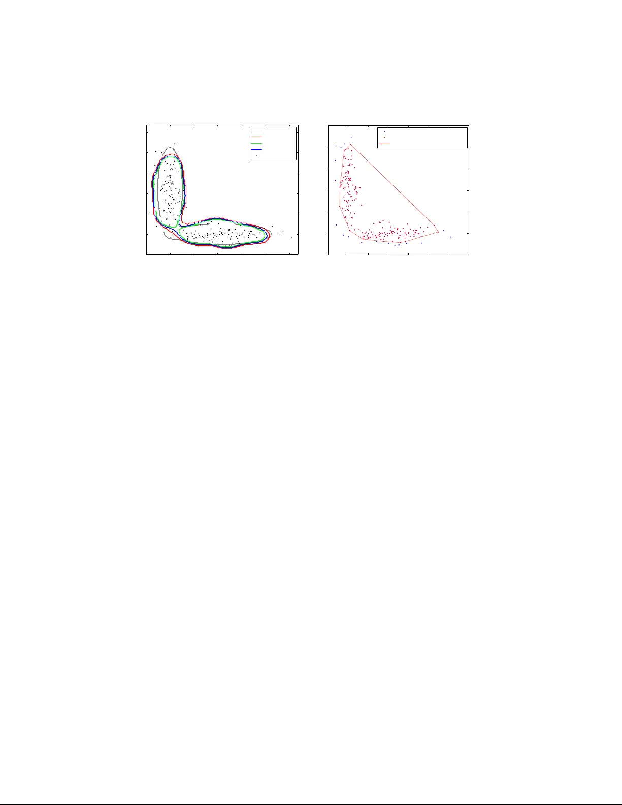
Submitte d to the Annals of Statistics arXiv: math.PR/0000000 EFFICIENT NONP ARAMETRIC CONF ORMAL PREDICTION REGIONS By Jing Lei ∗ , ‡ , James R obins § and Larr y W asserman † , ‡ Carne gie Mel lon University ‡ and Harvar d University § W e in vestigate and extend the conformal prediction metho d due to V ovk, Gammerman and Shafer ( 2005 ) to construct nonparametric prediction regions. These regions ha ve guaran teed distribution free, finite sample co v erage, without any assumptions on the distribution or the bandwidth. Explicit con vergence rates of the loss function are established for suc h reg ions under standard regularit y conditions. Ap- pro ximations for simplifying implemen tation and data driven band- width selection methods are also discussed. The theoretical prop erties of our metho d are demonstrated through simulations. 1. In tro duction. 1.1. Pr e diction r e gions and density level sets. Consider the follo wing pre- diction problem: w e observe iid data Y 1 , . . . , Y n ∈ R d from a distribution P and w e w ant to construct a prediction region C n = C n ( Y 1 , . . . , Y n ) ⊆ R d suc h that (1.1) P ( Y n +1 ∈ C n ) ≥ 1 − α for fixed 0 < α < 1 where P = P n +1 is the pro duct probability measure o v er the ( n + 1)-tuple ( Y 1 , . . . , Y n +1 ). 1 This is equiv alent to E [ P ( C n )] ≥ 1 − α where P ( C n ) is the probability mass of the random set C n . In other words, C n traps a future indep enden t observ ation Y n +1 ∼ P with probability at least 1 − α . The random set C n is called a (1 − α ) -pr e diction r e gion or a (1 − α ) -toler anc e r e gion . In this pap er we will use the name “prediction region” for consistency of presentation while “tolerance region” is often used as a synonym in the literature. Prediction is a ma jor fo cus of mac hine learning and statistics although the emphasis is often on p oint prediction. Prediction regions go b eyond ∗ Supp orted by NSF Grant BCS-0941518. † Supp orted by NSF Grant DMS-0806009 and Air F orce Grant F A95500910373. AMS 2000 subje ct classific ations: Primary 62G15; secondary 62G07 Keywor ds and phr ases: nonparametric prediction region, conformal prediction, k ernel densit y, efficiency 1 In general, we let P denote P n or P n +1 dep ending on the context. 1 imsart-aos ver. 2011/05/20 file: conformal_v1.tex date: October 18, 2018 2 J. LEI ET AL. merely pro viding a p oint prediction and are useful in a v ariet y of applications including quality con trol and anomaly detection. F or example, supp ose a sequence of items is b eing produced or observ ed. If one item falls out of the prediction region constructed from the previous samples, it indicates that this item is likely to b e differen t from the rest of the sample and some further in v estigation may b e necessary . Another application of prediction regions is data description and cluster- ing. Given a random sample from a distribution, it is often of interest to ask where most of the probability mass is concentrated. A natural answer to this question is the density level set L ( t ) = { y ∈ R d : p ( y ) ≥ t } , where p is the density function of P . When the distribution P is multimodal, a suitably chosen t will give a clustering of the underlying distribution ( Har- tigan , 1975 ). When t is given, consistent estimators of L ( t ) and rates of con v ergence ha ve b een studied in detail, for example, in Polonik ( 1995 ); Tsybak o v ( 1997 ); Baillo, Cuestas-Alb erto and Cuev as ( 2001 ); Baillo ( 2003 ); Cadre ( 2006 ); Willett and Now ak ( 2007 ); Rigollet and V ert ( 2009 ); Rinaldo and W asserman ( 2010 ). It often makes sense to define t implicitly using the desired probabilit y cov erage (1 − α ): (1.2) t ( α ) = inf n t : P ( L ( t )) ≥ 1 − α o . Let µ ( · ) denote the Lebesgue measure on R d . If the contour { y : p ( y ) = t ( α ) } has zero Leb esgue measure, then it is easily sho wn that C ( α ) := L ( t ( α )) = argmin C µ ( C ) , where the min is o ver  C : P ( C ) ≥ 1 − α  . Therefore, the density based clustering problem can sometimes b e formulated as estimation of the mini- m um volume prediction region. The study of prediction regions has a long history in statistics; see, for example Wilks ( 1941 ); W ald ( 1943 ); F raser and Guttman ( 1956 ); Chatterjee and Patra ( 1980 ); Di Bucchianico, Einmahl and Mushkudiani ( 2001 ); Cadre ( 2006 ); Li and Liu ( 2008 ). F or a thorough introduction to prediction regions, the reader is referred to the b o oks by Guttman ( 1970 ) and Aichison and Dunsmore ( 1975 ). In this paper we study a new er metho d due to V ovk, Gammerman and Shafer ( 2005 ) which w e describ e in Section 2 . 1.2. V alidity and efficiency. Let C n b e a prediction region. There are t wo natural criteria to measure its quality: validity and efficiency . By v alidit y w e mean that C n has the desired cov erage for all P , whereas by efficiency w e mean that C n is close to the optimal prediction region C ( α ) . imsart-aos ver. 2011/05/20 file: conformal_v1.tex date: October 18, 2018 NONP ARAMETRIC CONFORMAL PREDICTION 3 1.2.1. V alidity. By definition, a prediction region C n is a function of the sample ( Y 1 , ..., Y n ) and hence its cov erage P ( C n ) is a random quantit y . T o form ulate the notion of v alidity of a prediction region, F raser and Guttman ( 1956 ) defined (1 − α )-prediction regions with τ -confidence for C n satisfying (1.3) P ( P ( C n ) ≥ 1 − α ) ≥ τ . Ho w ever, ev aluating the exact probability in the ab ov e definition is rarely p ossible. Most work on nonparametric prediction regions v alidate their meth- o ds using an asymptotic version ( Chatterjee and Patra , 1980 ; Li and Liu , 2008 ): lim inf n →∞ P [ P ( C n ) ≥ 1 − α ] ≥ τ . On the other hand, if a pro cedure C n satisfies ( 1.1 ) for ev ery distribution P on R d and every n , then w e say that C n is a distribution fr e e pr e diction r e gion or has finite sample validity . 1.2.2. Efficiency. W e measure the efficiency of C n in terms of its close- ness to the optimal region C ( α ) . Recall that if P has a density p with resp ect to Leb esgue measure µ , then the smallest region with probability conten t at least 1 − α is (1.4) C ( α ) = { y : p ( y ) ≥ t ( α ) } , where t ( α ) is given b y ( 1.2 ), provided that the contour { y : p ( y ) = t ( α ) } has zero measure. Since p is unknown, C ( α ) cannot b e used as an estimator but only as a b enchmark in ev aluating the efficiency . W e define the loss function of C n b y (1.5) R ( C n ) = µ ( C n 4 C ( α ) ) where 4 denotes the symmetric set difference. Suc h loss functions ha v e been used, for example, by Chatterjee and Patra ( 1980 ) and Li and Liu ( 2008 ) in nonparametric prediction region estimation and by Tsybak o v ( 1997 ); Rigol- let and V ert ( 2009 ) in density level set estimation. Since, µ ( C n 4 C ( α ) ) = µ ( C n ) − µ ( C ( α ) ) + 2 µ ( C ( α ) \ C n ) ≥ µ ( C n ) − µ ( C ( α ) ) , it follows that the symmetric difference loss gives an upper b ound on the exc ess loss (1.6) E ( C n ) = µ ( C n ) − µ ( C ( α ) ) . imsart-aos ver. 2011/05/20 file: conformal_v1.tex date: October 18, 2018 4 J. LEI ET AL. In Chatterjee and P atra ( 1980 ) and Li and Liu ( 2008 ), a prediction region C n is called asymptotically minimal if (1.7) µ ( C n 4 C ( α ) ) P → 0 . Ho w ever, suc h an asymptotic prop erty does not sp ecify the rate of con- v ergence. While con vergence rate results are a v ailable for density level sets estimation (see Tsybako v , 1997 ; Rigollet and V ert , 2009 ; Mason and Polonik , 2009 , for example), relativ ely less is kno wn ab out prediction regions until recen tly ( Cadre , 2006 ; Samw orth and W and , 2010 ). 1.3. This p ap er. In this pap er, we prop ose an efficien t and easy to com- pute prediction region with finite sample v alidity and we study the rate of con v ergence of its loss. T o b e sp ecific, we construct C n suc h that: 1. C n satisfies ( 1.1 ) for all P and all n under no assumption other than iid . 2. F or any λ > 0, there exist constants c 1 ( λ, p ) and c 2 ( p ) indep enden t of n , such that (1.8) P R ( C n ) ≥ c 1 ( λ, p )  log n n  c 2 ( p ) ! = O ( n − λ ) , for densit y p satisfying some standard regularity conditions. 3. F or any y ∈ R d , the computation cost of ev aluating 1 ( y ∈ C n ) is linear in n . In other words, c hecking to see if a p oint y is in the prediction region, tak es linear time. The conv ergence rate of efficiency is describ ed by the term (log n/n ) c 2 ( p ) . W e give explicit formula of constant c 2 ( p ) in terms of the global smo othness and the local b ehavior of p near the con tour at level t ( α ). Its near optimalit y is discussed for some imp ortan t sp ecial cases. Our prediction region is obtained b y com bining the idea of conformal prediction ( V ovk, Gammerman and Shafer , 2005 ) with densit y estimation. W e first construct a conformal prediction region that is closely related to a kernel density estimator. The finite sample v alidity is inherited from the nature of conformal prediction regions. Then we show that suc h a region, whose analytical form ma y b e in tractable, is sandwiched by tw o k ernel den- sit y level sets with carefully tuned cut-off v alues. Therefore the efficiency of the conformal prediction region can b e approximated b y those of the tw o k ernel densit y lev el sets. As a by-product, we obtain a kernel density lev el set that alw a ys con tains the conformal prediction region, and hence also sat- isfies finite sample v alidit y . This observ ation means that, most of the time, imsart-aos ver. 2011/05/20 file: conformal_v1.tex date: October 18, 2018 NONP ARAMETRIC CONFORMAL PREDICTION 5 a k ernel density estimator will ha v e near optimal efficiency , finite sample v a- lidit y , and even low er computational cost at the same time. In the efficiency argumen t, we refine the rates of conv ergence for plug-in density level sets first developed in Cadre ( 2006 ), whic h may b e of indep endent interest. Our metho d in v olv es one tuning parameter which is the bandwidth in k ernel densit y estimation. W e giv e t wo practical data driven approaches to c ho ose the bandwidth and demonstrate the performance through sim ula- tions. 1.4. R elate d work. Our main technique for constructing prediction re- gions is inspired by the c onformal pr e diction metho d ( V o vk, Gammerman and Shafer , 2005 ; Shafer and V o vk , 2008 ), a general approach for construct- ing distribution free, sequen tial prediction regions using exc hangeabilit y . Al- though in its original appearance, conformal prediction is applied to sequen- tial classification and regression problems ( V o vk, Nouretdinov and Gammer- man , 2009 ), it is easy to adapt the metho d to the prediction task describ ed in ( 1.1 ). W e describ e this general metho d in Section 2 and our adaptation in Section 3 . In multiv ariate prediction region estimation, common approaches include metho ds based on statistical equiv alen t blo cks ( T ukey , 1947 ; Li and Liu , 2008 ) and plug-in density lev el sets ( Chatterjee and P atra , 1980 ; Cadre , 2006 ). In metho ds based on statistical equiv alen t blo cks, an ordering func- tion taking v alues in R 1 is defined and used to order the data p oints. Then one-dimensional tolerance interv al metho ds (e.g. Wilks , 1941 ) can b e ap- plied. Suc h methods usually give accurate cov erage but the efficiency is hard to prov e. In particular, Li and Liu ( 2008 ) prop osed an estimator using the m ultiv ariate spacing depth as the ordering function. Suc h a metho d is com- pletely nonparametric, requiring no tuning parameter, and is adaptive to the shap e of the underlying distribution if the densit y level sets are con vex. Ho w- ev er, this method requires O ( n d +1 ) time to compute the indicator 1 ( y ∈ C n ) for an y given y , which is muc h higher comparing to metho ds based on plug-in densit y level sets. Moreov er, it is not clear how this method p erforms when the lev el sets of underlying distribution are not conv ex. On the other hand, the methods based on plug-in densit y lev el sets ( Chatterjee and P atra , 1980 ) giv es prov able v alidity and efficiency in asymptotic sense regardless of the shap e of the distribution ( Cadre , 2006 ), while requiring only O ( n ) time to compute the indicator function. The p otential of such estimators has b een rep orted empirically in Di Bucchianico, Einmahl and Mushkudiani ( 2001 ): “ ... in principle the metho d based on density estimation can p erform very w ell if a prop er bandwidth is chosen, ...” imsart-aos ver. 2011/05/20 file: conformal_v1.tex date: October 18, 2018 6 J. LEI ET AL. Our approach, although originally inspired by conformal prediction, can b e view ed as a combination of the ordering based metho d and the density based metho d, where the ordering function is giv en by the estimated densit y . This agrees with the simple fact that the b est ordering function is just the densit y itself. T o the b est of our knowledge, this method is the first one with b oth finite sample v alidit y and explicit conv ergence rates. There are other metho ds for m ultiv ariate prediction regions. F or example, Di Bucc hianico, Einmahl and Mushkudiani ( 2001 ) prop osed to minimize the v olume ov er a pre-sp ecified class of sets while maintaining a minim um cov- erage under the empirical distribution. This metho d works well for common distributions whose level sets can b e well approximated b y regular shap es suc h as ellipsoids and rectangles. How ev er, its performance depends crucially on the pre-sp ecified sets which cannot b e very rich (must b e a Donsker class), and hence cannot b e guaran teed for arbitrary distributions. Moreov er, the minimization problem ma y be non-conv ex and hence computationally in ten- siv e. The rest of this pap er is organized as follo ws. In Section 2 w e introduce conformal prediction. In Section 3 we describ e a construction of prediction region by combining conformal prediction with k ernel densit y estimator. The appro ximation result (sandwic hing lemma) and asymptotic prop erties are also discussed in Section 3 . Practical metho ds for choosing the bandwidth are giv en in Section 4 and sim ulation results are presented in Section 5 . Some closing remarks and p ossible future w orks are giv en in Section 6 . Some tec hnical pro ofs are giv en in Section 7 . 2. Conformal prediction. W e can construct a v alid prediction region using a metho d from V o vk, Gammerman and Shafer ( 2005 ) and Shafer and V ovk ( 2008 ). Although their fo cus was on sequential prediction with co v ari- ates, the same basic idea can b e used here. The metho d is simple: consider a “conformit y measure” σ ( P , y ), which measures the “conformit y” or “agree- men t” of a p oint y with resp ect to a distribution P . Examples of such a function in the multiv ariate case include data depth (see Liu, Parelius and Singh , 1999 , and references therein), and the densit y function. F or other c hoices of conformit y measure, see the b o ok by V ovk, Gammerman and Shafer ( 2005 ). Giv en an indep endent sample Y 1 , ..., Y n from P , we test the h yp othesis that ( Y 1 , ..., Y n , Y n +1 ) iid ∼ P using observ ation ( Y 1 , ..., Y n , y ) for eac h y ∈ R d and inv ert the test. The test statistic is constructed using σ with P replaced by empirical distribution b P . When ( Y 1 , ..., Y n , Y n +1 ) is a random sample from P , let b P n +1 b e the corre- sp onding empirical distribution, whic h is symmetric in the n + 1 arguments. imsart-aos ver. 2011/05/20 file: conformal_v1.tex date: October 18, 2018 NONP ARAMETRIC CONFORMAL PREDICTION 7 Let π n +1 ,i = 1 n + 1 n +1 X j =1 1 h σ ( b P n +1 , Y j ) ≤ σ ( b P n +1 , Y i ) i . By symmetry , the sequence of random v ariables  σ ( b P n +1 , Y i ) : 1 ≤ i ≤ n + 1  are exchangeable and hence so are ( π n +1 ,i : 1 ≤ i ≤ n + 1). Let e α = b ( n + 1) α c n + 1 . Note that (1 + 1 /n ) − 1 α ≤ e α ≤ α and so e α ≈ α . Then, for an y α ∈ (0 , 1), (2.1) P ( π n +1 ,i ≥ e α ) ≥ 1 − α , since there are at least (1 − α )( n + 1) suc h π n +1 ,i ’s satisfying π n +1 ,i ≥ e α . Let (2.2) b C ( α ) ( Y 1 , ..., Y n ) = n y :  π n +1 ,n +1 | Y n +1 = y  ≥ e α o , where π n +1 ,n +1 | Y n +1 = y is the random v ariable π n +1 ,n +1 ev aluated at Y n +1 = y . Then ( 2.1 ) implies that P  Y n +1 ∈ b C ( α ) ( Y 1 , ..., Y n )  ≥ 1 − α. Based on the ab o v e discussion, an y conformity measure σ can b e used to construct prediction regions with finite sample v alidit y , with essentially no assumptions on P . The only requirement is exc hangeability of { π n +1 ,i } whic h is satisfied if the sample is indep endent. In this pap er we use (2.3) σ ( b P , y ) = b p ( y ) , that is, a densit y estimate ev aluated at y . W e sho w that such a choice is closely related to the plug-in density lev el set estimator and hence can b e pro v ed to b e asymptotically minimal with explicit rate of conv ergence. 3. Kernel density estimation. Let Y = ( Y 1 , . . . , Y n ). Define the aug- men ted data aug ( Y , y ) = ( Y 1 , . . . , Y n , y ). Let b p b e some densit y estimator that is defined for all n . F or example, b p could b e a parametric estimator or a nonparametric estimator suc h as a kernel density estimator. The particular algorithm we prop ose is giv en in Figure 1 . Recall that under the n ull hypothesis H 0 : ( Y 1 , ..., Y n , Y n +1 ) iid ∼ P , the ranks of b p ( Y i ) are exc hangeable, and hence P ( π ( y ) < e α ) ≤ α . Hence, we ha v e: imsart-aos ver. 2011/05/20 file: conformal_v1.tex date: October 18, 2018 8 J. LEI ET AL. Algo rithm 1: Conformal Prediction with Density Estimation Input: sample ( Y 1 , ..., Y n ), density estimator b p , and level α . F or every y : (a) Construct b p from aug ( Y , y ). (b) Compute σ 1 , . . . , σ n +1 where σ i = b p ( Y i ) for i = 1 , . . . , n and σ n +1 = b p ( y ). (c) T est the null hypothesis H 0 : Y n +1 ∼ P by computing the statistic π ( y ) = 1 n + 1 n +1 X i =1 1 ( σ i ≤ σ n +1 ) . Output: (inv erting the test) b C ( α ) = { y : π ( y ) ≥ e α } . Fig 1 . The algorithm for c omputing the pr ediction r e gion. Lemma 1 . Supp ose Y 1 , ..., Y n , Y n +1 is an indep endent r andom sample fr om P , then (3.1) P  Y n +1 ∈ b C ( α )  ≥ 1 − α , for al l pr ob ability me asur es P and henc e b C ( α ) is valid. Remark 2 . Note that the pr e diction r e gion is valid (has c orr e ct finite sample c over age) without any smo othness assumptions on p . Inde e d, the r e- gion is valid even if P do es not have a density. 3.1. Conformal pr e diction with kernel density estimation. No w w e turn to the combination of conformal prediction with k ernel density estimator. F or a giv en bandwidth h n and k ernel function K , let (3.2) b p n ( u ) = 1 n n X i =1 1 h d n K  u − Y i h n  b e the usual kernel density estimator. F or now, w e fo cus on a given band- width h n . The theoretical and practical asp ects of c ho osing h n will b e dis- cussed in Subsection 3.3 and Section 4 , resp ectiv ely . F or an y given y ∈ R d , let Y n +1 = y and define the augmented density estimator b p y n ( u ) = 1 h d n ( n + 1) n +1 X i =1 K  u − Y i h n  =  n n + 1  b p n ( u ) + 1 h d n ( n + 1) K  u − y h n  . (3.3) imsart-aos ver. 2011/05/20 file: conformal_v1.tex date: October 18, 2018 NONP ARAMETRIC CONFORMAL PREDICTION 9 No w we use the conformity measure σ ( b P n +1 , Y i ) = b p y n ( Y i ) and the p-v alue is π ( y ) = 1 n + 1 n +1 X i =1 1 ( b p y n ( Y i ) ≤ b p y n ( y )) . The resulting prediction region given by Algorithm 1 is b C ( α ) = { y : π ( y ) ≥ e α } . Figure 2 shows a one-dimensional example of the procedure, which w e will inv estigate in detail later. The top left plot shows a histogram of some data of sample size 20 from a tw o-component Gaussian mixture. The next three plots (top right, middle left, middle right) show three kernel density estimators with increasing bandwidth as well as the conformal prediction regions deriv ed from these estimators with α = 0 . 05. Ev ery bandwidth leads to a v alid region, but undersmo othing and ov ersmoothing lead to larger regions. The b ottom left plot shows the Leb esgue measure of the region as a function of bandwidth. The bottom right plot sho ws the estimator and prediction region based on the bandwidth whose corresponding conformal prediction region has the minimal Leb esque measure. 3.2. A n appr oximation. The conformal prediction region giv en by Algo- rithm 1 is closely related to the k ernel density estimator. In this subsection w e further inv estigate this connection and state the main appro ximation result, the sandwic hing lemma, which pro vides simple characterization of the conformal prediction region in terms of plug-in k ernel density level sets. The sandwiching lemma will also b e useful in the study of efficiency of the conformal prediction regions. W e first introduce some notation. Define the upp er and low er level sets of densit y p at lev el t , resp ectively: (3.4) L ( t ) = { y : p ( y ) ≥ t } , and L ` ( t ) = { y : p ( y ) ≤ t } . The corresp onding lev el sets of b p n are denoted L n ( t ) and L ` n ( t ), resp ectiv ely . Let (3.5) P y n = n n + 1 P n + 1 n + 1 δ y , where P n is the empirical distribution defined by the sample Y = ( Y 1 , ..., Y n ), and δ y is the p oint mass distribution at y . Define functions G ( t ) = P ( L ` ( t )) , G n ( t ) = P n ( L ` n ( t )) = n − 1 n X i =1 1 ( b p n ( Y i ) ≤ t ) , imsart-aos ver. 2011/05/20 file: conformal_v1.tex date: October 18, 2018 10 J. LEI ET AL. −5 0 5 0 1 2 3 4 5 −5 0 5 0.0 0.2 0.4 −5 0 5 0.00 0.06 0.12 −5 0 5 0.000 0.015 0.030 0 1 2 3 4 8 10 12 14 16 Bandwidth Lebesgue Measure −5 0 5 0.00 0.10 0.20 Fig 2 . T op left: histo gr am of some data. T op right, midd le left, and midd le right show thr e e kernel density estimators with incr e asing b andwidth as wel l as the conformal pr ediction r e gions derive d fr om these estimators. Bottom left: L eb esgue me asur e as a function of b andwidth. Bottom right: estimator and pr ediction r e gion fr om the b andwidth with smal lest pr e diction r e gion. imsart-aos ver. 2011/05/20 file: conformal_v1.tex date: October 18, 2018 NONP ARAMETRIC CONFORMAL PREDICTION 11 G y n ( t ) = P y n ( b p y n ( Y ) ≤ t ) = ( n + 1) − 1 n X i =1 1 ( b p y n ( Y i ) ≤ t ) + 1 ( b p y n ( y ) ≤ t ) ! . The functions G , G n and G y n defined abov e are the cum ulativ e distribu- tion function (CDF) of p ( Y ) and its empirical v ersions with sample Y and aug ( Y , y ), resp ectiv ely . By ( 2.2 ) and Algorithm 1, the conformal prediction region can b e written as (3.6) b C ( α ) = n y ∈ R d : G y n ( b p y n ( y )) ≥ e α o . Let Y (1) , . . . , Y ( n ) b e the reordered data so that b p n ( Y (1) ) , . . . , b p n ( Y ( n ) ) are in ascending order. Let i n,α = b ( n + 1) α c , and define the inner and outer sandwic hing sets: L − n = L n  b p n ( Y ( i n,α ) )  and L + n = L n  b p n ( Y ( i n,α ) ) − ( nh d ) − 1 ψ K  , where ψ K = sup u,u 0 | K ( u ) − K ( u 0 ) | . Then we ha ve the following “sandwic h- ing” lemma, whose pro of can b e found in Subsection 7.1 . Lemma 3 (Sandwic hing Lemma) . Assume that || K || ∞ = K (0) , then (3.7) L − n ⊆ b C ( α ) ⊆ L + n . According to the sandwic hing lemma, L + n also guarantees distribution free finite sample cov erage and it is easier to analyze. The inner region, L − n , whic h is not m uc h smaller than L + n when n is large, generally do es not hav e finite sample v alidit y . W e confirm this through sim ulations in Section 5 . Next we in v estigate the efficiency of these prediction regions. 3.3. Asymptotic pr op erties. In this subsection we pro v e asymptotic effi- ciency of b C ( α ) and the sandwic hing sets in terms of the con v ergence rates of their loss. Recall that the optimal prediction region at level 1 − α can b e written as (3.8) C ( α ) = L ( t ( α ) ) = { y : p ( y ) ≥ t ( α ) } , where t ( α ) is the cut-off v alue of the density function so that the probability mass in the low er lev el set is exactly α : (3.9) G ( t ( α ) ) = P ( p ( Y ) ≤ t ( α ) ) = α. imsart-aos ver. 2011/05/20 file: conformal_v1.tex date: October 18, 2018 12 J. LEI ET AL. This holds if we assume G is con tinuous at t ( α ) so that the ab ov e equation implies P ( p ( Y ) ≥ t ( α ) ) = 1 − α . This is equiv alent to assuming that the con tour of p at v alue t ( α ) , { y : p ( y ) = t ( α ) } , has zero measure under P . The inner and outer sandwiching sets L − n and L + n are plug-in estimators of density level sets of the form: (3.10) L n ( t ( α ) n ) = { y : b p n ( y ) ≥ t ( α ) n } , where t ( α ) n = b p n ( Y ( i n,α ) ) for the inner set L − n and t ( α ) n = b p n ( Y ( i n,α ) ) − ( nh d n )) − 1 ψ K for the outer set L + n . Here w e can view t ( α ) n as an estimate of t ( α ) . In Cadre, Pelletier and Pudlo ( 2009 ) it is shown that, under regu- larit y conditions of the density p , the plug-in estimators t ( α ) n and L n ( t ( α ) n ) using k ernel density estimator are consisten t with con vergence rate 1 / p nh d n for a range of h n . Here, we refine the results using a set of slightly mo dified conditions. In tuitiv ely sp eaking, for any density estimator b p n and cut-off v alues t ( α ) n , the plug-in density level set L n ( t ( α ) n ) is an accurate estimator of L ( t ( α ) ) if: 1. The estimated density function, b p n , is close to the true density p . 2. The true density is not to o flat around lev el t ( α ) . 3. The estimated cut-off v alue t ( α ) n is an accurate estimate of t ( α ) . The first condition has b een extensiv ely studied in the literature of nonpara- metric density estimation and sufficient conditions of conv ergence for kernel densit y estimators in v arious forms hav e b een established. The second con- dition is more sp ecific for densit y lev el set estimation. A common condition is the γ -exp onent at lev el t ( α ) , whic h is first in tro duced by Polonik ( 1995 ) and has b een used by man y others (see Tsybako v , 1997 ; Rigollet and V ert , 2009 , for example). The third condition is somewhat opp osite to the second one. It essen tially requires that the densit y function cannot b e too steep near the true cut-off v alue. This turns out to b e a natural condition whenever the densit y has b ounded deriv ativ es near the contour. W e formalize this condi- tion through a “mo dified γ -exp onent condition” which is detailed in Section 3.3.2 . 3.3.1. H¨ older Classes of Densities. T o study the efficiency of the predic- tion region, we need some smo othness condition on p . The H¨ older class is a p opular smo othness condition in nonparametric inferences ( Tsybako v , 2009 , Section 1.2). Here we use the version given in Rigollet and V ert ( 2009 ). Let s = ( s 1 , ..., s d ) be a d -tuple of non-negativ e in tegers and | s | = s 1 + ... + imsart-aos ver. 2011/05/20 file: conformal_v1.tex date: October 18, 2018 NONP ARAMETRIC CONFORMAL PREDICTION 13 s d . F or an y x ∈ R d , let x s = x s 1 1 · · · x s d d and D s b e the differential op erator: D s f = ∂ | s | f ∂ x s 1 1 · · · ∂ x s d d ( x 1 , ..., x d ) . Giv en β > 0, for any functions f that are b β c times differentiable, denote its T aylor expansion of degree b β c at x 0 b y f ( β ) x 0 ( x ) = X | s |≤ β ( x − x 0 ) s s 1 ! · · · s d ! D s f ( x 0 ) . Definition 4 (H¨ older class) . F or c onstants β > 0 , L > 0 , define the H¨ older class Σ( β , L ) to b e the set of b β c -times differ entiable functions on R d such that, (3.11) | f ( x ) − f ( β ) x 0 ( x ) | ≤ L || x − x 0 || β . 3.3.2. The γ -exp onent c ondition. F or a density function p , and a lev el t ∈ (0 , || p || ∞ ), the usual γ -exp onent condition requires that there exists an  0 > 0 and c 1 > 0 such that (3.12) µ ( { y : t < p ( y ) ≤ t +  } ) ≤ c 1  γ , ∀  ∈ (0 ,  0 ) . Condition ( 3.12 ) is essen tially requiring that the density p ( y ) increases roughly at rate  1 /γ when y mov es aw a y from the con tour by an  distance. As a re- sult, a larger v alue of γ corresp onds to a faster change of the density p when mo ving aw ay from the contour, hence it is easier to estimate the density lev el set. In this pap er, we consider the mo dified γ -exp onen t condition: Definition 5 (Mo dified γ -exp onent condition) . We say a density func- tion p satisfies the mo difie d γ -exp onent c ondition at level t , if ther e exist c onstants  0 > 0 and c 1 , c 2 > 0 , such that (3.13) c 1 ≤ P ( { y : t − ≤ p ( y ) ≤ t + } ) ( t + − t − ) γ ≤ c 2 , ∀ t −  0 ≤ t − < t + ≤ t +  0 . The mo dified γ -exp onent condition differs from the original definition in three asp ects: 1. First, it allows b oth sides of the interv al to change within a neigh b or- ho o d of t , whic h is stronger than ( 3.12 ). It do es not allow the con tour at level t to ha v e positive measure. W e note that if the con tour at lev el t has p ositive measure, then the estimated level set has at least a constant loss unless the cut-off v alue is estimated without error. imsart-aos ver. 2011/05/20 file: conformal_v1.tex date: October 18, 2018 14 J. LEI ET AL. 2. Second, it do es not only require an upp er b ound on the measure, but also a lo wer b ound. Since the upp er b ound indicates that the density cannot b e to o flat around the contour, the low er b ound do es not allo w the density to b e to o steep. This condition implies that the estimated cut-off v alue is close to the truth. It usually holds when the densit y is smo oth enough around the contour. F or example, when the con tour at level t is smo oth and the density p satisfies | p ( y ) − t | ≈ δ 1 /γ for all y that is δ aw a y from the contour and all δ small enough ( Tsybako v , 1997 ). 3. Moreo v er, in the mo dified condition, w e use the measure induced by p , rather than the Leb esgue measure. This is a minor difference since w e alwa ys ha ve, for all t −  0 ≤ t − < t + ≤ t +  0 , t −  0 ≤ P ( { y : t − < p ( y ) ≤ t + } ) µ ( { y : t − < p ( y ) ≤ t + } ) ≤ t +  0 . 3.3.3. Conditions on the Kernel. A standard condition on the kernel is the notion of β -v alid k ernels. Definition 6 ( β -v alid kernel) . F or any β > 0 , a function K : R d 7→ R 1 is a β -valid kernel if 1. K is supp orte d on [ − 1 , 1] d . 2. R K = 1 . 3. R | K | r < ∞ , al l r ≥ 1 . 4. R y s K ( y ) dy = 0 for al l 1 ≤ | s | ≤ β . In the literature, β -v alid kernels are usually used with H¨ older class of functions to deriv e fast rate of conv ergence. The existence of univ ariate β - v alid kernels can b e found in ( Tsybako v , 2009 , Section 1.2). A multiv ariate β -v alid kernel can b e obtained by taking direct pro duct of univ ariate β -v alid k ernels. 3.3.4. Asymptotic pr op erties of estimate d density level set. Consider the follo wing assumptions: Assumption A1: (a) The density function p ∈ P ( β , L ), where P ( β , L ) is the class of all densit y functions that are in the H¨ older class Σ( β , L ). (b) The density p satisfies the mo dified γ -exp onent condition at lev el t ( α ) . (c) The density function p is uniformly b ounded by a constan t ¯ L . imsart-aos ver. 2011/05/20 file: conformal_v1.tex date: October 18, 2018 NONP ARAMETRIC CONFORMAL PREDICTION 15 Assumption A2: The bandwidth satisfies (3.14) h n   log n n  1 2 β + d . Assumption A3: The kernel K is β -v alid and || K || ∞ = K (0). These assumptions extend those in ( Cadre, P elletier and Pudlo , 2009 ), where β = 1 is considered. Also A1(b) considered here is a lo cal version. The next theorem states the qualit y of cut-off v alues used in the sand- wic hing sets L − n and L + n . Theorem 7 . L et t ( α ) n = b p n ( Y ( i n,α ) ) , wher e b p n is the kernel density es- timator given by e q. ( 3.2 ), and Y ( i ) and i n,α ar e define d as in Se ction 3.2 . Under assumptions A1-A3, for any λ > 0 , ther e exist c onstants A λ , A 0 λ dep ending only on p , K and α , such that (3.15) P | t ( α ) n − t ( α ) | ≥ A λ  log n n  β 2 β + d + A 0 λ  log n n  1 2 γ ! = O ( n − λ ) . W e giv e the pro of of Theorem 7 in Section 7.2 . Theorem 7 is useful for establishing the con v ergence of the corresp onding level set. Observing that ( nh d n ) − 1 = o ((log n/n ) β / (2 β + d ) ), it follo ws immediately that the cut-off v alue used in L + n also satisfies ( 3.15 ). The next theorem giv es the rate of conv er- gence for plug-in level set estimators when the cut-off v alue satisfies ( 3.15 ). Theorem 8 . L et t ( α ) n b e a r andom se quenc e which satisfies ( 3.15 ). Under A1-A3, for any λ > 0 , ther e exist c onstants B λ , B 0 λ dep ending on p , K and α only, such that P µ ( L n ( t ( α ) n ) 4 C ( α ) ) ≥ B λ  log n n  β γ 2 β + d + B 0 λ  log n n  1 2 ! = O ( n − λ ) . By Theorem 7 , the cut-off v alues used in L − n and L + n b oth satisfy ( 3.15 ), so the conv ergence rate in Theorem 8 holds for L − n and L + n . By Lemma 3 , it also holds for b C ( α ) . Corollar y 9 . Under A1-A3, for any λ > 0 , ther e exists c onstant B λ , B 0 λ dep ending on p , K and α only, such that, for al l b C ∈ { b C ( α ) , L − n , L + n } , (3.16) P µ ( b C 4 C ( α ) ) ≥ B λ  log n n  β γ 2 β + d + B 0 λ  log n n  1 2 ! = O ( n − λ ) . imsart-aos ver. 2011/05/20 file: conformal_v1.tex date: October 18, 2018 16 J. LEI ET AL. In the most common case β = γ = 1, the term (log n/n ) β γ / (2 β + d ) domi- nates the conv ergence rate. If w e further assume that the level set L ( t ( α ) ) is star-shap ed (or more generally , a union of star-shap ed sets), then the rate giv en by Corollary 9 is near optimal, up to a logarithm term. Indeed, the rate in equation ( 3.16 ) is within a logarithm term of the minimax risk for densit y level set estimation as dev elop ed in Tsybak o v ( 1997 ). But note that the problem considered here is harder than estimating density lev el set at a fixed lev el since the cut-off v alue is not known in adv ance and needs to b e estimated. Indeed, the logarithm term comes from estimating t ( α ) n . W e also note that the con tin uity condition on p is slightly different than that in Tsybak o v ( 1997 ) where it is assumed that the density con tour at the desired lev el is in a H¨ older class. But the same construction of the low er b ound can b e used under the global smo othness conditions A1(a) and A1(b). A minimax risk rate of the plug-in density lev el set at a fixed level has b een dev elop ed by Rigollet and V ert ( 2009 ). Although the rate is similar as that obtained in this paper, the construction of the lo wer b ound only applies to fixed cut-off v alues close to 1, and hence has only limited application to the range of α v alues of practical in terest. 4. Cho osing the bandwidth. As illustrated in Figure 2 , the efficiency of b C ( α ) dep ends on the c hoice of h n . The size of estimated prediction region can b e v ery large if the bandwidth is either to o large or to o small. There- fore, in practice it is desirable to c ho ose a go o d bandwidth in an automatic and data driven manner. In k ernel density estimation, the c hoice of band- width has b een one of the most imp ortant topics and man y approac hes hav e b een studied; see Loader ( 1999 ) and Mammen et al. ( 2011 ) and references therein. Intuitiv ely , a goo d densit y estimator b p will lik ely lead to a goo d prediction region, and the dep endence on n of the (near) optimal choice of h n in Theorem 8 is similar to that in the con text of kernel densit y estima- tion. How ev er, this is not quite the case ( Sam w orth and W and , 2010 ). The in tuition is simple: F or densit y estimation, a go o d bandwidth guaran tees the accuracy of estimated density in the whole space, whereas for level sets it suffices to estimate the density accurately near the contour. W e prop ose tw o practical metho ds to c ho ose a go o d bandwidth from a giv en candidate set H = { h 1 , . . . , h m } , based on the idea that a go o d prediction region has small Leb esgue measure; see Figures 3 and 4 . The metho ds introduced here are applicable to an y prediction region estimator b C with finite sample v alidit y . In b oth approac hes, we compute the prediction region for eac h h ∈ H and choose the one with the smallest volume. T o preserv e finite sample v alidit y , the first approach, describ ed in Fig 3 , uses a imsart-aos ver. 2011/05/20 file: conformal_v1.tex date: October 18, 2018 NONP ARAMETRIC CONFORMAL PREDICTION 17 Algo rithm 2: T uning with Bonferroni Correction Input: sample Y = ( Y 1 , ..., Y n ), prediction region estimator b C , and level α . 1. Construct prediction sets { b C h = b C h ( Y 1 , ..., Y n ) : h ∈ H} each at level 1 − α/m , where m = |H| . 2. Let b h = argmin h µ ( b C h ). 3. Return b C b h . Fig 3 . Algorithm 2: b andwidth selection. Bonferroni correction. Proposition 10 . If b C satisfies finite sample validity for any h , then the estimate d pr e diction r e gion b C b h given by A lgorithm 2 also satisfies finite sample validity. Proof. Using Bonferroni correction we ha v e P ( Y n +1 ∈ b C b h ) ≥ P ( Y n +1 ∈ b C h , ∀ h ∈ H ) ≥ 1 − X h ∈H P ( Y n +1 / ∈ b C h ) ≥ 1 − α , where the last inequality uses the fact that each b C h is a finite sample v alid prediction region at level 1 − α/m . When m = |H | is large, Algorithm 2 tends to b e conserv ative since each single b C h has cov erage 1 − α/m , which could b e muc h bigger than the ideal (1 − α ) region. The algorithm describ ed in Figure 4 uses sample splitting and only sacrifices a constant rate of efficiency regardless of |H| . Proposition 11 . If b C satisfies finite sample validity for al l h , then b C b h, 2 , the output of Algorithm 3, also satisfies finite sample validity. Proof. Note that b h is indep endent of Y 2 , as a result, E  P  b C b h, 2   = E  E  P  b C b h, 2    b h  ≥ E  1 − α | b h  =1 − α . imsart-aos ver. 2011/05/20 file: conformal_v1.tex date: October 18, 2018 18 J. LEI ET AL. Algo rithm 3: T uning With Sample Splitting Input: sample Y = ( Y 1 , ..., Y n ), prediction region estimator b C , and level α 1. Split the sample randomly into tw o equal sized subsamples, Y 1 and Y 2 . 2. Construct prediction regions { b C h, 1 : h ∈ H} each at level 1 − α , using subsample Y 1 . 3. Let b h = argmin h µ ( b C h, 1 ). 4. Return b C b h, 2 , which is constructed using bandwidth b h and subsample Y 2 . Fig 4 . Algorithm 3: b andwidth selection. It is easy to see that these metho ds hav e small excess loss with high prob- abilit y since, b y construction, µ ( b C ) ≤ µ ( b C h ∗ ) + ν n , where h ∗ is the best bandwidth that minimizes the excess loss E ( µ ( b C h )) and ν n is a negligible term, b ecause for H dense enough, there exists h j ∈ H such that h j ≈ h ∗ . Although minimizing excess loss do es not necessarily minimize the symmet- ric difference loss, a small excess loss itself is a desired prop erty in practice and is also a necessary condition of small symmetric difference loss. How ever, a more detailed relationship b et ween excess loss and symmetric difference loss requires extra conditions and w e leav e that for future research. 5. Numerical example. A simple illustration of Algorithm 1 is pre- sen ted in Figure 2 . Here we consider a tw o-dimensional Gaussian mixture, whose geometric structure allo ws a better visualization of the results. W e also test the bandwidth selectors presen ted in Section 4 . Due to the small v alue of α and limited sample size, w e find Algorithm 3 more preferable than Algorithm 2. Th us we only present the results using bandwidth chosen by sample splitting. F or example, when n = 200, 100 data p oints are used to select the bandwidth and the other 100 data p oints are used to construct the prediction region using the selected bandwidth. T able 1 shows the co v erage and Leb esgue measure of the prediction region of lev el .90 ov er 1,000 rep etitions. The co verage is excellent and the size of the region is close to optimal. Both the conformal region b C ( α ) and the outer sandwic hing set L + n giv es correct cov erage regardless of the sample size. It is worth noting that the inner sandwiching set L − n do es not giv e the desired co v erage, which suggests that decreasing the cut-off v alue in L + n is not merely an artifact of pro of, but a necessary tuning. The observ ed excess loss also reflects a rate of conv ergence that supp orts our theoretical results on the symmetric difference loss. T aking b C ( α ) for example, in Corollary 9 w e ha v e imsart-aos ver. 2011/05/20 file: conformal_v1.tex date: October 18, 2018 NONP ARAMETRIC CONFORMAL PREDICTION 19 T able 1 The simulation r esults for 2-d Gaussian mixtur e with α = 0 . 1 over 1000 r ep etitions. The L eb esgue me asur e of the ide al r egion ≈ 28 . 02 . Co verage Leb esgue Measure n = 200 n = 1000 n = 200 n = 1000 b C ( α ) 0 . 897 ± 0 . 002 0 . 900 ± 0 . 001 34 . 3 ± 0 . 31 31 . 1 ± 0 . 15 L − n 0 . 882 ± 0 . 001 0 . 896 ± 0 . 001 34 . 1 ± 0 . 22 32 . 2 ± 0 . 10 L + n 0 . 900 ± 0 . 001 0 . 907 ± 0 . 001 36 . 9 ± 0 . 21 34 . 1 ± 0 . 10 β = γ = 1, d = 2, and p (log 200) / 200 p (log 1000) / 1000 ≈ 1 . 9 , whic h agrees with the observed drop of av erage excess loss from 6 to 3 as n increased from 200 to 1,000. Figure 5 sho ws a t ypical realization of the estimators. In b oth panels, the dots are data p oin ts when n = 200. The left panel shows the conformal prediction region with sample splitting (blue curv e), together with the inner and outer sandwic hing sets (red and green curv es, respectively). Also plotted is the ideal region C ( α ) (the grey curve). It is clear that all three estimated regions captures the main part of the ideal region, and they are mutually close. On the right panel we plot a realization of the depth based approach from Li and Liu ( 2008 ). This approac h do es not require an y tuning param- eter. How ev er, it tak es O ( n d +1 ) time to ev aluate 1 ( y ∈ b C ) for an y single y . In practice it is recommended to compute the empirical depth only for all the data p oin ts and use the conv ex hull of all data p oin ts with high depth as the estimated prediction region. As can be seen on the picture, suc h a con v ex hull construction misses the “L” shap e of the ideal region. Moreov er, the k ernel densit y method is at least 1,000 times faster than the depth based metho d in our implementation ev en when n = 200. Figure 6 shows the effect of bandwidth on the excess loss based on a typi- cal implemen tation of conformal prediction, where the y axis is the Leb esgue measure of the estimated region. W e observe that for the conformal predic- tion region b C ( α ) , the excess loss is stable for a wide range of bandwidth, esp ecially that mo derate undersmo othing do es not harm the p erformance v ery muc h. An intuitiv e explanation is that the data near the contour is dense enough to allo w for mo derate undersmo othing. Similar phenomenon should b e exp ected whenever α is not too small. Moreo ver, the selected bandwidth from the outer sandwiching set L + n is close to that obtained from the conformal region. This observ ation ma y b e of practical interest since it is usually muc h faster to compute L + n . imsart-aos ver. 2011/05/20 file: conformal_v1.tex date: October 18, 2018 20 J. LEI ET AL. y (1 ) y (2) −2 0 2 4 6 8 10 −2 0 2 4 6 8 10 Optimal Set Outer Bound Inner Bound Conformal Set Data Point −2 0 2 4 6 8 10 12 −2 0 2 4 6 8 10 y (1 ) y (2) Data points not in region Data points in region convex hull of data poins in region Fig 5 . Conformal pr e diction r e gion (left) and the c onvex hul l of the multivariate sp acing depth b ase d toler anc e r e gion (right), with data fr om a two-comp onent Gaussian mixtur e. 6. Conclusion. W e hav e constructed a distribution free prediction re- gion by combining ideas from densit y estimation and conformal prediction. It can also b e viewed as a combination of the statistically equiv alent blo ck metho ds and the density level set metho ds. The region is easy to compute and, under regularit y conditions, is asymptotically near optimal. Even with- out the regularity conditions, the region retains its finite sample v alidity . The bandwidth tuning algorithm (Algorithm 3) used in our sim ulation resem bles cross-v alidation, a p opular device for kernel density estimators. In Algorithm 3, the comparison b et ween candidate bandwidths is based on a direct ev aluation of loss, that is, the Leb esgue measure of the estimated region. This feature yields both conceptually and computationally simple implemen tation which is also highly stable as observ ed in our simulation studies. F uture topics of research in this asp ect include understanding the theoretical prop erties of suc h a bandwidth selector, its connection with other approac hes in the literature of densit y and lev el set estimation, and the p erformance under b oth excess loss as w ell as the symmetric difference loss. In current w ork we are studying nonparametric procedures that adapt to smo othness conditions. In principle it is p ossible to further develop this metho d to deal with nonparametric prediction with co v ariates or parametric mo dels. imsart-aos ver. 2011/05/20 file: conformal_v1.tex date: October 18, 2018 NONP ARAMETRIC CONFORMAL PREDICTION 21 0 0.5 1 1.5 2 2.5 3 3.5 4 0 10 20 30 40 50 60 70 80 log 2 ( h/h n ) µ ( ˆ C ) µ ( ˆ C ) µ ( ˜ C − ) µ ( ˜ C + ) 0 0.5 1 1.5 2 2.5 3 3.5 4 0 10 20 30 40 50 60 70 80 log 2 ( h/h n ) µ ( ˆ C ) µ ( ˆ C ) µ ( ˜ C − ) µ ( ˜ C + ) Fig 6 . L eb esgue me asur e of the conformal pr e diction r e gion versus b andwidth for the Gaus- sian mixtur e data with n = 200 (left) and n = 1000 (right). Here h n = p (log n ) /n . 7. Pro ofs. 7.1. Pr o of of L emma 3 . Proof of the sandwiching lemma. The pro of is done via a direct c haracterization of L − n and L + n . First, for each y ∈ L − n and i ≤ i n,α , we hav e b p y n ( y ) − b p y n ( Y ( i ) ) = n n + 1  b p n ( y ) − b p n ( Y ( i ) )  + 1 ( n + 1) h d  K (0) − K  Y ( i ) − y h  ≥ 0 . As a result, G y n ( b p y n ( y )) ≥ i n,α / ( n + 1) = e α and hence y ∈ b C ( α ) . Similarly , for eac h y / ∈ L + n and i ≥ i n,α w e hav e b p y h ( y ) − b p y h ( Y ( i ) ) = n n + 1  b p h ( y ) − b p h ( Y ( i ) )  + 1 ( n + 1) h d  K (0) − K  Y ( i ) − y h  ≤ n n + 1  b p h ( y ) − b p h ( Y ( i n,α ) )  + 1 ( n + 1) h d ψ K < 0 . Therefore, G y n ( b p y n ( y )) ≤ ( i n,α − 1) / ( n + 1) < e α and hence y / ∈ b C ( α ) . imsart-aos ver. 2011/05/20 file: conformal_v1.tex date: October 18, 2018 22 J. LEI ET AL. 7.2. Pr o of of The or em 7 . Pr eliminaries. Recall that L ` ( t ) is the lo w er level set of p at level t : { y ∈ R d : p ( y ) ≤ t } . The bias in the estimated cut-off level t ( α ) n can b e b ounded in terms of tw o quan tities: V n = sup t> 0 | P n ( L ` ( t )) − P ( L ` ( t )) | , and R n = || b p n − p || ∞ . Here V n can b e viewed as the maximum of the empirical pro cess P n − P o v er a nested class of sets, and R n is the L ∞ loss of the density estimator. As a result, V n can b e b ounded using the standard empirical pro cess and V C dimension argumen t, and R n can b e b ounded using the smo othness of p and k ernel K with a suitable choice of bandwidth. F ormally , we provide upp er b ounds for these tw o quantities through the following lemma. Lemma 12 . L et V n , R n b e define d as ab ove, then under assumptions A1- A3, for any λ > 0 , ther e exist c onstants A 1 ,λ and A 2 ,λ dep ending on λ only, such that, P V n ≥ A 1 ,λ r log n n ! = O ( n − λ ) , and P R n ≥ A 2 ,λ  log n n  β 2 β + d ! = O ( n − λ ) . Proof. First, it is easy to c hec k that the class of sets { L ` ( t ) : t > 0 } are nested with VC (V apnik-Chervonenkis) dimension 2 and hence by classical empirical pro cess theory (see, for example, v an der V aart and W ellner , 1996 , Section 2.14), there exists a constan t C 0 > 0 such that for all η > 0 (7.1) P ( V n ≥ η ) ≤ C 0 n 2 exp( − nη 2 / 32) . Let η = A p log n/n , we hav e P  V n ≥ A p log n/n  ≤ C 0 n 2 exp( − A 2 log n/ 32) = C 0 n − ( A 2 / 32 − 2) . (7.2) The first result then follows b y choosing A 1 ,λ = p 32( λ + 2). imsart-aos ver. 2011/05/20 file: conformal_v1.tex date: October 18, 2018 NONP ARAMETRIC CONFORMAL PREDICTION 23 Next we b ound R n . Let ¯ p = E [ b p n ], and  n =  log n n  β 2 β + d . By triangle inequality R n ≤ || b p n − ¯ p || ∞ + || ¯ p − p || ∞ . Due to a result of Gin ´ e and Guillou ( 2002 ) (see also equation (49) in Chapter 3 of Prak asa Rao , 1983 ), under the assumptions A1(c) and A3, there exist constan ts C 1 , C 2 and B 0 > 0 such that ha v e for all B ≥ B 0 , P ( k b p n − ¯ p k ∞ ≥ B  n ) ≤ C 1 exp( − C 2 B 2 log( h − 1 n )) = C 1 h C 2 B 2 n . (7.3) On the other hand, by assumptions A1(a) and A3, for some constant C 3 (7.4) k ¯ p − p k ∞ ≤ C 3 h β n . W e note that in the inequalities ( 7.2 ), ( 7.3 ) and ( 7.4 ) the constants C i , i = 0 , ..., 3, dep end on p and K only . Hence, (7.5) P ( || b p − p || ∞ ≥ ( C 3 + B )  n ) ≤ C 1 h C 2 B 2 n , whic h concludes the second part by choosing A 2 ,λ = C 3 + s (2 β + d ) λ C 2 . Proof of Theorem 7 . Let α n = i n,α /n = b ( n + 1) α c /n . W e hav e | α n − α | ≤ 1 /n . Recall that the ideal level t ( α ) can b e written as t ( α ) = G − 1 ( α ) , where the function G is the cum ulativ e distribution function of p ( Y ), as defined in Subsection 3.2 . By the modified γ -exp onent condition the inv erse imsart-aos ver. 2011/05/20 file: conformal_v1.tex date: October 18, 2018 24 J. LEI ET AL. of G is well defined in a small neigh b orho o d of α . When n is large enough, w e can define t ( α n ) as t ( α n ) = G − 1 ( α n ) . Again, b y the mo dified γ -exp onent, c 1 | t ( α n ) − t ( α ) | γ ≤ | G ( t ( α n ) ) − G ( t ( α ) ) | = | α n − α | ≤ n − 1 . Therefore, for n large enough (7.6) | t ( α n ) − t ( α ) | ≤ ( c 1 n ) − 1 /γ . Equation ( 7.6 ) allo ws us to switch to the problem of b ounding | t ( α ) n − t ( α n ) | . Recall that t ( α ) n = b p n ( Y ( i n,α ) ). The key of the pro of is to observ e that t ( α ) n = G − 1 n ( α n ) := inf { t : G n ( t ) ≥ α n } . Then it suffices to sho w that G − 1 and G − 1 n are close at α n . In fact, b y definition of R n w e hav e for all t > 0: L ` ( t − R n ) ⊆ L ` n ( t ) ⊆ L ` ( t + R n ) . Applying the empirical measure P n to each term in the ab ov e: P n ( L ` ( t − R n )) ≤ P n ( L ` n ( t )) ≤ P n ( L ` ( t + R n )) . By definition of V n , P ( L ` ( t − R n )) − V n ≤ P n ( L ` n ( t )) ≤ P ( L ` ( t + R n )) + V n . By definition of G and G n , the ab ov e inequalit y b ecomes G ( t − R n ) − V n ≤ G n ( t ) ≤ G ( t + R n ) + V n . Let W n = R n + (2 V n /c 1 ) 1 /γ . Supp ose n is large enough such that  c 1 n  1 γ + 2 A 1 ,λ c 1 r log n n ! 1 γ <  0 , then on the even t V n ≤ A 1 ,λ q log n n , G n  t ( α n ) − W n  ≤ G  t ( α n ) − W n + R n  + V n imsart-aos ver. 2011/05/20 file: conformal_v1.tex date: October 18, 2018 NONP ARAMETRIC CONFORMAL PREDICTION 25 = G  t ( α n ) − (2 V n /c 1 ) 1 /γ  − G  t ( α n )  + α n + V n ≤ α n − V n < α n . where the last inequalit y uses the left side of the modified γ -exp onen t condition. Similarly , G n ( t ( α n ) + W n ) > α n . Hence, for n large enough, if V n ≤ A 1 ,λ p (log n ) /n then, (7.7) | t ( α ) n − t ( α n ) | ≤ W n . T o conclude the pro of, first note that  c 1 n  1 γ = o  log n n  1 2 γ ! . Then we can find c onstan t A 0 λ suc h that for all n large enough, (7.8) A 0 λ −  2 A 1 ,λ c 1  1 γ !  log n n  1 2 γ ≥  c 1 n  1 γ . Let A λ = A 2 ,λ . Combini ng equations ( 7.6 ) and ( 7.7 ), on the even t (7.9) E n,λ := ( R n ≤ A λ  log n n  β 2 β + d , V n ≤ A 1 ,λ  log n n  1 2 ) , w e hav e, for n large enough, | t ( α ) n − t ( α ) | ≤| t ( α ) n − t ( α n ) | +  c 1 n  1 γ ≤ W n +  c 1 n  1 γ ≤ R n + (2 c − 1 1 V n ) 1 /γ +  c 1 n  1 γ ≤ A λ  log n n  β 2 β + d + 2 A 1 ,λ c 1 r log n n ! 1 γ +  c 1 n  1 γ ≤ A λ  log n n  β 2 β + d + A 0 λ  log n n  1 2 γ , (7.10) where the second last inequalit y is from the definition of E n,λ and the last inequalit y is from the c hoice of A 0 λ . The pro of is concluded by observing P ( E c n,λ ) = O ( n − λ ), a consequence of Lemma 12 . imsart-aos ver. 2011/05/20 file: conformal_v1.tex date: October 18, 2018 26 J. LEI ET AL. 7.3. Pr o of of The or em 8 . Proof of Theorem 8 . In the pro of we write t n for t ( α ) n . Observe that µ  L n ( t n ) 4 C ( α )  = µ n b p n ≥ t n , p < t ( α ) o + µ n b p n < t n , p ≥ t ( α ) o . (7.11) Note that n b p n ≥ t n , p < t ( α ) o ⊆ n t ( α ) − | t n − t ( α ) | − R n ≤ p < t ( α ) o , (7.12) and n b p n < t n , p ≥ t ( α ) o ⊆ n t ( α ) < p ≤ t ( α ) + | t ( α ) − t n | + R n o . (7.13) Therefore L n ( t n ) 4 C ( α ) ⊆ n t ( α ) − | t n − t ( α ) | − R n < p ≤ t ( α ) + | t ( α ) − t n | + R n o . (7.14) Supp ose n is large enough such that 2 A 2 ,λ  log n n  β 2 β + d + A 0 λ  log n n  1 2 γ <  0 ∧ t ( α ) 2 ! , where the constant A 2 ,λ is defined as in Lemma 12 and A 0 λ is defined as in equation ( 7.8 ). Then on the even t E n,λ as defined in equation ( 7.9 ), applying Theorem 7 and condition ( 3.13 ) on the right hand side of ( 7.14 ) yields µ  L n ( t n ) 4 C ( α )  ≤ P  L n ( t n ) 4 C ( α )  t ( α ) − | t n − t ( α ) | − R n ≤ 2 t ( α ) c 2 2 A 2 ,λ  log n n  β 2 β + d + A 0 λ  log n n  1 2 γ ! γ ≤ B λ  log n n  β γ 2 β + d + B 0 λ  log n n  1 2 , (7.15) where B λ , B 0 λ are p ositive constants depend only on p , K , α and γ . imsart-aos ver. 2011/05/20 file: conformal_v1.tex date: October 18, 2018 NONP ARAMETRIC CONFORMAL PREDICTION 27 References. Aichison, J. and Dunsmore, I. R. (1975). Statistic al Pr e diction Analysis . Cambridge Univ. Press. Baillo, A. (2003). T otal error in a plug-in estimator of lev el sets. Statistics & Pr ob ability L etters 65 411-417. Baillo, A. , Cuest as-Alber to, J. and Cuev as, A. (2001). Conv ergence rates in non- parametric estimation of level sets. Statistics & Pr ob ability L etters 53 27-35. Cadre, B. (2006). Kernel estimation of densit y lev el sets. Journal of multivariate analysis 97 999-1023. Cadre, B. , Pelletier, B. and Pudlo, P. (2009). Clustering by estimation of density lev el sets at a fixed probability. man uscript. Cha tterjee, S. K. and P a tra, N. K. (1980). Asymptotically minimal multiv ariate tol- erance sets. Calcutta Statist. Asso c. Bul l. 29 73-93. Di Bucchianico, A. , Einmahl, J. H. and Mushkudiani, N. A. (2001). Smallest non- parametric tolerance regions. The Annals of Statistics 29 1320-1343. Fraser, D. A. S. and Guttman, I. (1956). T olerance regions. The Annals of Mathemat- ic al Statistics 27 162-179. Gin ´ e, E. and Guillou, A. (2002). Rates of strong uniform consistency for m ultiv ariate k ernel densit y estimators. Annales de l’Institut Henri Poinc ar e (B) Pr ob ability and Statistics 38 907-921. Guttman, I. (1970). Statistic al T oler anc e R egions: Classic al and Bayesian . Griffin, Lon- don. Har tigan, J. (1975). Clustering Algorithms . John Wiley , New Y ork. Li, J. and Liu, R. (2008). Multiv ariate spacings based on data depth: I. construction of nonparametric multiv ariate tolerance regions. The Annals of Statistics 36 1299-1323. Liu, R. , P arelius, J. and Singh, K. (1999). Multiv ariate analysis by data depth: de- scriptiv e statistics, graphics and inference. The Annals of Statistics 27 783-858. Loader, C. (1999). Bandwidth selection: classical or plug-in? The A nnals of Statistics 27 415-438. Mammen, E. , Miranda, M. D. M. , Nielsen, J. P . and Sperlich, S. (2011). Do- V alidation for k ernel density estimation. Journal of the Americ an Statistic al Asso ciation 106 651-660. Mason, D. M. and Polonik, W. (2009). Asymptotic normality of plug-in level set esti- mates. The Annals of Applie d Pr ob ability 19 1108-1142. Polonik, W. (1995). Measuring mass concen trations and estimating density contour clus- ters - an excess mass approac h. The Annals of Statistics 23 855-881. Prakasa Rao, B. L. S. (1983). Nonp ar ametric F unctional Estimation . Academic Press. Rigollet, P. and Ver t, R. (2009). Optimal rates for plug-in estimators of denslty level sets. Bernoul li 14 1154-1178. Rinaldo, A. and W asserman, L. (2010). Generalized density clustering. The Annals of Statistics 38 2678-2722. Samwor th, R. J. and W and, M. P. (2010). Asymptotics and optimal bandwidth selection for highest density region estimation. The Annals of Statistics 38 1767-1792. Shafer, G. and Vo vk, V. (2008). A tutorial on conformal prediction. Journal of Machine L e arning R ese ar ch 9 371-421. Tsybako v, A. (1997). On nonparametric estimation of density level sets. The Annals of Statistics 25 948-969. Tsybako v, A. (2009). Intr o duction to nonpar ametric estimation . Springer. Tukey, J. (1947). Nonparametric estimation, I I. Statistical equiv alent blocks and m ulti- imsart-aos ver. 2011/05/20 file: conformal_v1.tex date: October 18, 2018 28 J. LEI ET AL. v arate tolerance regions. The Annals of Mathematic al Statistics 18 529-539. v an der V aar t, A. W. and Wellner, J. A. (1996). We ak Conver genc e and Empiric al Pr o c esses . Springer. V ovk, V. , Gammerman, A. and Shafer, G. (2005). Algorithmic L e arning in a R andom World . Springer. V ovk, V. , Nouretdinov, I. and Gammerman, A. (2009). On-line preditive linear re- gression. The Annals of Statistics 37 1566-1590. W ald, A. (1943). An extension of Wilks metho d for setting tolerance limits. The A nnals of Mathematic al Statistics 14 45-55. Wilks, S. (1941). Determination of sample sizes for setting tolerance limits. The Annals of Mathematic al Statistics 12 91-96. Willett, R. M. and Now ak, R. D. (2007). Minimax optimal lev el-set estimation. IEEE T r ansactions on Image Pr o c essing 16 2965 - 2979. Dep ar tment of St a tistics Carnegie Mellon University Pittsburgh, Pennsyl v ania 15213 USA E-mail: jinglei@andrew.cmu.edu larry@stat.cmu.edu Dep ar tment of Epidemiology Har v ard School of Public Heal th 677 Huntington A venue Boston, Massachusetts 02115 USA E-mail: robins@hsph.harv ard.edu imsart-aos ver. 2011/05/20 file: conformal_v1.tex date: October 18, 2018