$ell_0$ Minimization for Wavelet Frame Based Image Restoration

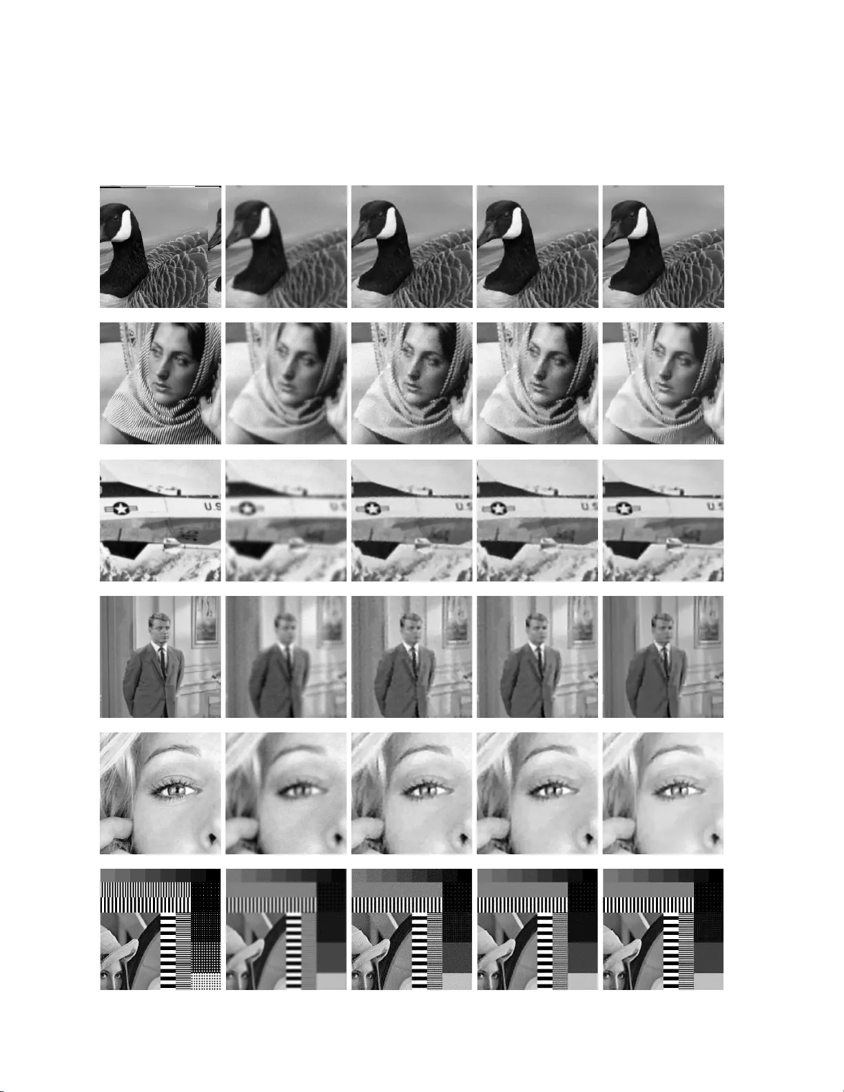
ℓ 0 MINIMIZA TION F OR W A VELET FRAME BASED IMA GE RESTORA TION YONG ZHANG, BIN DONG, AND ZHAOSONG LU Abstract. The theory of (tigh t) wa v elet f r ames has b een extensive ly studied in the past tw en t y y ears and they a re curren tly widely used for image restoration and other image pro cessing and analysi s problems. The success of wa v elet fr ame based models, including balanced approac h [18, 7] and analysis based approach [11, 31, 50 ] , is due to their capabilit y of sparsely approximating piecewise sm ooth functions lik e images. Motiv at ed by the balanced approac h and analysis based approach, we shall prop ose a wa v elet frame based ℓ 0 minimization model, where the ℓ 0 “norm” of the frame coefficien ts is penalized. W e adap t the penalty decomposition (PD) metho d of [40] to solve the prop osed optimization problem. Some con ve rgence analysis of the adapted PD method wil l also b e provided. Numerical results show ed that the prop osed mo del solved b y the PD method can gene rate images with b etter quality than those obtained by either analysis based approac h or balanced approach in terms of restoring s harp features as well as main taining smoothness of the recov ered i m ages. 1. Introduction Mathematics ha s b een playing an important role in the mo dern dev elopments of ima ge pro ces sing and analysis. Image r estoration, including image denoising, deblurring, inpain ting, to mo graphy , etc., is one of the mos t imp ortant areas in image proc e s sing and analysis. Its ma jor purp ose is to enhance the qualit y of a given image that is corrupted in v arious ways during the pro cess of imaging, ac quisition and communication; and enable us to see cr ucial but subtle ob jects residing in the imag e . Therefore, image restor ation is an impo rtant step to take tow ards accur ate in terpretations of the physical world and making optimal decisio ns. 1.1. Image Restoration. Imag e restor ation is often fo r m ulated as a linear inverse problem. F or the sim- plicit y of the notations, we denote the images as vectors in R n with n e quals to the total num ber of pixels. A typical imag e restoratio n problem is formulated as (1.1) f = Au + η , where f ∈ R d is the observed imag e (or measur e ments), η denotes white Gaussian noise with v ariance σ 2 , and A ∈ R d × n is some linear op erator. The ob jectiv e is to find the unknown true imag e u ∈ R n from the observed image f . Typically , the linear op era tor in (1 .1) is a conv o lutio n oper ator for ima g e deco n volution problems, a pr o jection op erator for image inpainting and par tial Rado n transfo rm for computed tomog raphy . T o solve u fr om (1.1), one of the mo st natural choices is the follo wing least square problem min u ∈ R n k Au − f k 2 2 , where k · k 2 denotes the ℓ 2 -norm. This is, how ever, not a go o d idea in g eneral. T ak ing ima g e deconv o lution problem as an ex ample, since the matrix A is ill-co nditioned, the noise η po ssessed by f will b e amplified a fter solving the above least squa res problem. Therefor e, in order to s uppress the effect of nois e and a lso preserve key features of the image, e.g ., edges, v a rious reg ularization bas ed o ptimization mo dels w ere prop os e d in the literature. Among all regularization bas ed mo dels for image restoratio n, v ariationa l metho ds and wa v elet frames based appro aches a re widely adopted and hav e been pro ven successful. The tr end of v a riational methods and partial differential equatio n (PDE) based image pro c essing started with the refined Rudin-Osher- F atemi (ROF) mo del [45] which p enalizes the total v a riation (TV) of u . Many of the current PDE based metho ds for image denoising and decompos ition utilize TV regula rization for its 2000 Mathematics Subje ct Classific ation. 80M50, 90C26, 42C40, 68U10. Key wor ds and phr ases. ℓ 0 minimization, hard thresholding, wa velet fr ame, image restoration. The firs t and thir d authors were supp orted in part by NSERC Di sco v ery Gran t. 1 2 YONG ZHANG, BIN DONG, AND ZHAOSONG LU bene fic ia l e dge pres e rving prop erty (see e.g ., [41, 46, 42]). The ROF mo del is e spec ia lly effective on restor ing images that are piecewise constant, e.g ., binary images . Other types o f v ariational mo dels were a ls o pro po sed after the ROF mo del. W e refer the interested rea ders to [36, 17, 41, 42, 22, 2, 23, 53] and the references therein for mor e details. W av elet frame bas ed appro aches are relatively ne w and came from a differen t path. The basic idea for wa velet frame based approa c hes is that images can b e spar sely approximated by prop erly designed wa velet frames, and hence, the regula r ization used for wav e le t frame based mo de ls is the ℓ 1 -norm of fra me co efficients. Although wa velet frame based approaches take similar forms as v ariational metho ds, they were generally considered as different approa ches tha n v ariational methods b ecause, amo ng many other reasons , wa velet frame based approa c hes is defined for discrete data, while v ariational methods a ssume all v ariable s are functions. Some studies in the literatur e (see for example [51]) indicated that there was a relation be t ween Haa r wa velet and total v aria tion. How ever, it was not clear if there exists a genera l r elation betw een wa velet frames and v ar iational models (with general differen tial op erators ) in the con text of image restora tions. In a recent pap er [9], the a uthors esta blished a rigoro us connectio n betw een o ne o f the wav elet frame based approa c hes, namely the analysis based approach, a nd v ariationa l mo dels. It was sho wn in [9] that the a nalysis based approa ch can be regarded as a finite difference approximation of a certain type of general v a r iational mo del, and such approximation will be ex act when ima ge r esolution go es to infinit y . F urthermor e, through Gamma-co nv er g ence, the authors s howed that the solutions of the analysis based approach also approximate the so lutions o f the co rresp onding v ariational model. Suc h connections no t only grant geometric interpretation to w av elet frame based appr oaches, but also lead to even wider a pplications of them, e.g., image segmen tation [27] and 3D surfac e rec o nstruction from unorganized point sets [29]. On the other hand, the discr e tization pr ovided b y w av elet frames was shown, in e.g., [18, 20, 10, 11, 9, 28], to be superio r than the standard discretiza tions fo r some of the v a r iational mo de ls , due to the multiresolution structure and re dundancy of w av e le t frames whic h enable wa velet frame based mo dels to a daptively choose a prop er differential o per ators in differen t regio ns o f a giv en image accor ding to the or der o f the singularity of the underlying solutions . F or these reasons, as well as the fact that digital images are alwa ys discrete, we use wa velet frames as the to o l for image res toration in this paper . 1.2. W av elet F rame Based Approac hes. W e now briefly introduce the concept of tigh t frames and tight w av elet frame, and then recall so me of the frame based image restor ation mo dels. In teresting r eaders should consult [44, 24, 25] for theories o f fr ames a nd w a velet frames, [47] for a short survey on theory a nd applications of frames, and [28] for a more detailed survey . A countable set X ⊂ L 2 ( R ) is called a tight frame of L 2 ( R ) if f = X h ∈ X h f , h i h ∀ f ∈ L 2 ( R ) , where h· , ·i is the inner pr o duct of L 2 ( R ). The tight fra me X is calle d a tight wav elet fra me if the elements of X are ge ne r ated b y dilations and translations of finitely many functions called framelets . The constr uction of fra melets can b e obtained by the unitary extension pr inc iple (UEP) of [44]. In our implemen tations, we will mainly use the piecewise linear B-spline framelets cons tructed by [44]. Given a 1- dimensional framele t system for L 2 ( R ), the s -dimensional tight wa velet frame system for L 2 ( R s ) can b e eas ily constructed by using tensor pro ducts of 1 - dimensional framelets (see e.g., [24, 28]). In the discr ete setting, we will use W ∈ R m × n with m ≥ n to denote fa s t tenso r product framelet decomp osition and use W ⊤ to deno te the fast reconstr uction. Then b y the unitar y extensio n principle [44], we have W ⊤ W = I , i.e., u = W ⊤ W u for a n y image u . W e will further denote an L -level fra mele t decomp osition of u as W u = ( . . . , W l,j u, . . . ) ⊤ for 0 ≤ l ≤ L − 1 , j ∈ I , where I denotes the index set of all framelet bands and W l,j u ∈ R n . Under such notation, w e hav e m = L × |I | × n . W e will also us e α ∈ R m to denote the frame co efficients, i.e., α = W u , where α = ( . . . , α l,j , . . . ) ⊤ , with α l,j = W l,j u. More details on discrete alg orithms of framelet trans fo rms c an be found in [28]. ℓ 0 MINIMIZA TION F OR W A VE LET FRAME BASED IMAGE RESTORA TION 3 Since tight wav e le t frame systems are re dunda n t systems (i.e., m > n ), the repres en tation of u in the fra me domain is not unique. Therefor e, there are mainly three formulations utilizing the sparsenes s of the frame co efficients, namely , analysis ba sed appro ach, syn thesis based appr oach, and bala nce d approach. Detailed and in tegrated descr iptions of these three metho ds can b e found in [2 8]. The wa velet frame based image pro cess ing started from [18, 19] for high-reso lution image reco nstructions, where the pro pos ed a lgorithm was later analyzed in [7]. These work lea d to the following balanced appr oach [8] (1.2) min α ∈ R m 1 2 k AW ⊤ α − f k 2 D + κ 2 k ( I − W W ⊤ ) α k 2 2 +        L − 1 X l =0   X j ∈I λ l,j | α l,j | p   1 /p        1 , where p = 1 or 2, 0 ≤ κ ≤ ∞ , λ l,j ≥ 0 is a sca la r parameter , and k · k D denotes the w eighted ℓ 2 -norm with D po sitive definite. This for m ulation is referred to as the balanced appro a ch b ecause it balances the spar sit y of the frame co efficient and the smoo thness of the image. The balanced appr oach (1.2 ) was applied to v arious applications in [16, 21, 48, 3 9]. When κ = 0 , only the sparsity of the frame co efficient is penalized. This is called the syn thesis based approach, as the image is synthesized b y the s parsest co efficient vector(see e.g., [26, 32, 33, 34, 35]). When κ = + ∞ , only the sparsity of canonical wa velet fr ame co efficients, which cor resp onds to the s moo thness of the underlying image, is p enalized. F or this cas e , pr o blem (1.2) can b e rewritten as (1.3) min u ∈ R n 1 2 k Au − f k 2 D +        L − 1 X l =0   X j ∈I λ l,j | W l,j u | p   1 /p        1 . This is c alled the ana lysis based a pproach, as the co efficient is in range of the analy s is o per ator (see, for example, [11, 31, 50]). Note that if w e take p = 1 for the la st term of (1.2) and (1.3), it is known as the anisotro pic ℓ 1 -norm of the frame co efficients, whic h is the cas e used for earlier frame based image r estoration mo dels. The ca se p = 2 , called isotr opic ℓ 1 -norm of the frame coefficie nts, w as pr op osed in [9] and w a s shown to b e superior than anisotr opic ℓ 1 -norm. Therefore , we will c ho o se p = 2 for our simulations. 1.3. Mo tiv ations and Contributions. F or mos t of the v ariational mo dels a nd w av elet frame based a p- proaches, the c hoice of no rm for the r egularizatio n term is the ℓ 1 -norm. T a king w av ele t frame based ap- proaches for exa mple, the attempt o f minimizing the ℓ 1 -norm of the fra me co efficients is to increase their sparsity , which is the r ight thing to do s inc e piecewise s moo th functions like images can b e spa r sely ap- proximated by tight wav elet frames. Although the ℓ 1 -norm of a vector does not dir ectly corresp ond to its cardinality in contrast to ℓ 0 “norm”, it can b e re g arded as a conv ex approximation to ℓ 0 “norm”. Such approximation is also an excellent approximation fo r many cases. It was shown b y [12], which gener alizes the exciting results of compressed sensing [13, 15, 14, 30], that for a given w av elet frame, if the oper a tor A satisfies cer tain conditions, and if the unknown true image can b e spa rsely appr oximated by the given wav e let frame, one can ro bustly r ecov er the unkno wn image b y pena lizing the ℓ 1 -norm of the frame co efficients. F or image restora tio n, how ev er, the conditions on A as required by [12] are not generally satisfied, which means p enalizing ℓ 0 “norm” and ℓ 1 -norm may pro duce different s olutions. Although b oth the balanced approach (1.2) and a nalysis bas ed appr oach (1.3) can generate restored ima ges with very high quality , one natural question is whether us ing ℓ 0 “norm” instead of ℓ 1 -norm can further improve the results. On the other hand, it w as obs erved, in e.g., [2 8] (also see Figure 3 a nd Figure 4), that balanced appr oach (1.2) gener ally generates images with sharp er features like e dg es than the analys is ba sed approa ch (1.3), bec ause balanced a pproach emphasizes more on the spa rsity of the fra me coefficients. How ever, the recov- ered imag es from ba lanced appr o ach usually cont ains more artifact (e.g., oscillatio ns ) than ana lysis based approach, b ecause the reg ularization term of the analysis based appr oach ha s a direct link to the regularity of u (as pr ov en b y [9 ]) comparing to balanc e d approach. Although such trade- off can b e controlled by the parameter κ in the ba lanced appro ach (1.2) , it is not very easy to do in pra ctice. F urthermore, when a large 4 YONG ZHANG, BIN DONG, AND ZHAOSONG LU κ is c hosen, some of the numerical a lgorithms solving (1.2) will conv erge slow er than choosing a smaller κ (see e.g., [48, 2 8]). Since p enaliz ing ℓ 1 -norm of W u ensures s mo o thness w hile not as m uch sparsity as bala nced a pproach, we prop ose to penalize ℓ 0 “norm” of W u instea d. In tuitiv ely , this should provide us a ba lance b etw een sharpness of the featur e s and s moo thness for the recovered images. The difficulty here is that ℓ 0 minimization problems a re generally hard to solve. Recen tly , pe na lt y decompos ition (PD) metho ds w ere pro po sed by [40] for a general ℓ 0 minimization problem that can b e used to solve our propos ed model due to its generality . Computational results of [40] demo ns trated that their methods gener ally outp erform the existing metho ds for compressed sensing proble ms , sparse logistic regression and sparse inv erse co v aria nce selection proble ms in ter ms of quality o f so lutions a nd/or computationa l efficiency . This motiv ates us to adapt one of their PD metho ds to so lve our prop osed ℓ 0 minimization problem. Sa me a s prop osed in [40], the blo ck co ordinate descent (BCD) metho d is used to solve each p enalty subpro blem of the PD metho d. How e ver, the co n vergence analysis o f the BCD metho d was missing from [4 0] when ℓ 0 “norm” app ears in the ob jectiv e function. Indeed, the conv ergence o f the BCD metho d generally requires the contin uity of the ob jectiv e function as discussed in [52]. In addition, the B CD metho d for the optimization pro blem with the nonconv ex ob jectiv e function has only been prov ed to conv er ge to a stationar y po in t which is not a lo cal minimizer in g eneral (see [52] for details). Con tributions. The main contributions of this pap er are summarized as follows. 1) W e pro po se a new wa velet fr ame ba s ed mo del for image restoration pro blems that penalize s the ℓ 0 “norm” of the wa velet fra me co efficients. Numerical simulations show that the PD metho d that solves the propo sed mo del generates recov er ed images with b etter quality than those obta ined by either balanced approa ch and analysis based appr o ach. 2) Given the discontin uit y and nonconvexit y of the ℓ 0 “norm” term in the ob jectiv e function, we have prov ed so me con vergence results for the BCD method which is missing from the literatur e. W e no w lea ve the details of the mo del and a lgorithm to Section 2 a nd details of simulations to Section 3. 2. Model and A lgorithm W e start by in tro ducing some simple notations. The spa ce o f symmetric n × n matrices will be denoted by S n . If X ∈ S n is po sitive definite, we write X ≻ 0. W e deno te by I the identit y matrix, whose dimension should be clear from the context. Giv en a n index set J ⊆ { 1 , . . . , n } , x J denotes the sub-vector for med b y the entries of x indexed by J . F or any real v ector, k · k 0 and k · k 2 denote the cardinality (i.e., the num ber of nonzero entries) and the Euclidean norm o f the vector, resp ectively . In addition, k x k D denotes the w eight ed ℓ 2 -norm defined by k x k D = √ x ⊤ D x with D ≻ 0. 2.1. Mo del. W e no w prop ose the following o ptimiza tion model for image restoratio n problems, (2.1) min u ∈Y 1 2 k Au − f k 2 D + X i λ i k ( W u ) i k 0 , where Y is some con vex subset of R n . Here w e are using the m ulti-index i and denote ( W u ) i (similarly for λ i ) the v a lue of W u at a g iven pixe l lo c a tion within a certain level a nd band of wav e le t frame tra nsform. Comparing to the analysis based mo del, we are now penalizing the n umber of no nzero elements of W u . As men tioned earlier that if we emphas ize to o muc h on the spa rsity of the fr a me co efficie nts a s in the balanced approach or synthesis bas ed appro ach, the recovered image will co ntain ar tifacts, although features like edges will b e sharp; if we emphasiz e to o m uch o n the r egularity o f u like in analysis ba sed approa c h, features in the recov ered images will b e slight ly blurre d, although ar tifacts and nois e will b e nicely suppressed. Therefore, by p enalizing the ℓ 0 “norm” of W u as in (2.1), w e can indeed achieve a b etter balance b etw een s harpness of features and smo othness of the r ecov ered images . Given that the ℓ 0 “norm” is an in teger-v alued, discontin uous and noncon v ex function, pro blem (2.3) is g e nerally har d to so lve. Some a lg orithms pro p os ed in the literature, e.g., iterative hard thresholding algorithms [5 , 6, 38], cannot b e directly applied to the pro po sed mo del (2.1) unless W = I . Recently , Lu and ℓ 0 MINIMIZA TION F OR W A VE LET FRAME BASED IMAGE RESTORA TION 5 Zhang [40] prop osed a p enalty de c o mpo sition (PD) method to solve the following general ℓ 0 minimization problem: (2.2) min x ∈X f ( x ) + ν k x J k 0 for some ν > 0 controlling the sparsity of the solution, where X is a clo sed conv ex set in R n , f : R n → R is a con tin uously differentiable function, and k x J k 0 denotes the c ardinality of the sub vector for med b y the ent ries of x indexe d by J . In view of [4 0], w e reformulate (2.1) as (2.3) min u ∈Y ,α = W u 1 2 k Au − f k 2 D + X i λ i k α i k 0 and then we can adapt the PD metho d o f [40] to tackle problem (2.1) directly . Same as pr op o sed in [40], the BCD method is used to solve each penalty subproblem of the P D metho d. In addition, we apply the non-monotone gr a dient pro jection metho d prop osed in [4] to solve one of the subpr oblem in the BCD metho d. 2.2. Alg orithm for Problem (2.3) . In this section, we discuss how the P D metho d prop osed in [4 0] solving (2.2) can b e a da pted to solve problem (2.3). Letting x = ( u 1 , . . . , u n , α 1 , . . . , α m ), J = { n + 1 , . . . , n + m } , ¯ J = { 1 , . . . , n } , f ( x ) = 1 2 k Ax ¯ J − f k 2 D and X = { x ∈ R n + m : x J = W x ¯ J and x ¯ J ∈ Y } , we can clearly see that the pr oblem (2.3) ta kes the sa me form as (2.2). In addition, ther e obviously exists a fea sible p oint ( u feas , α feas ) for pro blem (2.3) when Y 6 = ∅ , i.e. there exist ( u feas , α feas ) suc h that W u feas = α feas and u feas ∈ Y . In particular, we can choo s e ( u feas , α feas ) = (0 , 0), which is the choice we mak e for our numerical studies. W e now discuss the implemen tation details of the PD method when so lv ing the pro po sed wav elet frame based mo del (2.3). Given a p enalty parameter  > 0 , the asso cia ted quadr atic penalty function for (2.3) is defined as (2.4) p  ( u, α ) := 1 2 k Au − f k 2 D + X i λ i k α i k 0 +  2 k W u − α k 2 2 . Then we have the following PD metho d for pro blem (2.3) where each penalty subproblem is appr oximately solved by a BCD metho d (see [40] for details). P e nalt y Decomp osi tion (PD) Metho d for (2 .3) : Let  0 > 0, δ > 1 b e given. Choos e an arbitrar y α 0 , 0 ∈ R m and a constant Υ such that Υ ≥ max { 1 2 k Au feas − f k 2 D + P i λ i k α feas i k 0 , min u ∈Y p  0 ( u, α 0 , 0 ) } . Set k = 0. 1) Set q = 0 and apply the BCD metho d to find an approximate solution ( u k , α k ) ∈ Y × R m for the pena lt y subproblem (2.5) min { p  k ( u, α ) : u ∈ Y , α ∈ R m } by p erforming steps 1a )-1d): 1a) Solve u k,q +1 ∈ Arg min u ∈Y p  k ( u, α k,q ). 1b) Solve α k,q +1 ∈ Arg min α ∈ R n p  k ( u k,q +1 , α ). 1c) If ( u k,q +1 , α k,q +1 ) satis fies the stopping criteria of the BCD metho d, set ( u k , α k ) := ( u k,q +1 , α k,q +1 ) and go to step 2). 1d) Otherwise, set q ← q + 1 a nd go to step 1a ). 2) If ( u k , α k ) satis fies the s topping criteria o f the PD metho d, stop and output u k . Otherwise, set  k +1 := δ  k . 3) If min u ∈Y p  k +1 ( u, α k ) > Υ, set α k +1 , 0 := α feas . Otherwise, set α k +1 , 0 := α k . 4) Set k ← k + 1 and g o to step 1). end 6 YONG ZHANG, BIN DONG, AND ZHAOSONG LU Remark 2.1 . In the pr actic al implementation, we terminate the inner iter ations of t he BCD metho d b ase d on the r elative pr o gr ess of p  k ( u k,q , α k,q ) whi ch c an b e describ e d as follows: (2.6) | p  k ( u k,q , α k,q ) − p  k ( u k,q +1 , α k,q +1 ) | max( | p  k ( u k,q +1 , α k,q +1 ) | , 1) ≤ ǫ I . Mor e over, we terminate t he out er iter ations of the PD metho d onc e (2.7) k W u k − α k k 2 max( | p  k ( u k , α k ) | , 1) ≤ ǫ O . Next we discuss how to solve tw o subproblems arising in step 1a ) and 1b) of the PD metho d. 2.2.1. The BCD subpr oblem in step 1a). The BCD s ubproblem in step 1a) is in the form o f (2.8) min u ∈Y 1 2 h u, Qu i − h c, u i for some Q ≻ 0 and c ∈ R n . Obviously , when Y = R n , problem (2.8) is an unconstr ained qua dratic progra mming pr oblem that can be solv ed b y the conjugate gradient method. Nevertheless, the pixel v a lues of an image ar e usually b ounded. F o r example, the pixel v alues of a CT image should be alwa ys g r eater than o r equal to zer o and the pixel v alues of a grayscale image is betw e en [0 , 255]. Then the co rresp onding Y of these t wo exa mples are Y = { x ∈ R n : x i ≥ l b ∀ i = 1 , . . . , n } with l b = 0 and Y = { x ∈ R n : lb ≤ x i ≤ ub ∀ i = 1 , . . . , n } with l b = 0 and ub = 25 5. T o s o lve these t yp es of the constrained quadratic programming problems, we a pply the no nmonotone pro jected g r adient metho d prop osed in [4] and terminate it using the duality ga p and dual fea sibilit y conditions (if neces sary). F or Y = { x ∈ R n : x i ≥ l b ∀ i = 1 , . . . , n } , given a Lagr angian multiplier β ∈ R n , the asso ciated Lag r angian dual function of (2.8) can b e written a s: L ( u, β ) = w ( u ) + β ⊤ ( lb − u ) , where w ( u ) = 1 2 h u, Qu i − h c, u i . Based on the Ka rush-Kuhn-T uc ker (KKT) conditions, for an optimal solution u ∗ of (2.8), there exists a Lagrangian m ultiplier β ∗ such that Qu ∗ − c − β ∗ = 0 , β ∗ i ≥ 0 ∀ i = 1 , . . . , n , ( lb − u ∗ i ) β ∗ i = 0 ∀ i = 1 , . . . , n . Then at the s th iteration of the pr o jected g r adient metho d, w e let β s = Qu s − c . A s { u s } approaches the solution u ∗ of (2.8), { β s } approaches the Lagr angian multiplier β ∗ and the corre s po nding duality gap a t each itera tion is given by P n i =1 β s i ( lb − u s i ). Therefore, we terminate the pro jected g radient metho d when | P n i =1 β s i ( lb − u s i ) | max( | w ( u s ) | , 1) ≤ ǫ D and − min( β s , 0) max( k β s k 2 , 1) ≤ ǫ F for some tolerance s ǫ D , ǫ F > 0. F or Y = { x ∈ R n : l b ≤ x i ≤ u b ∀ i = 1 , . . . , n } , given La grangia n multipliers β , γ ∈ R n , the a sso ciated Lagra ng ian function of (2.8) can be written as: L ( u, β , γ ) = w ( u ) + β ⊤ ( lb − u ) + γ ⊤ ( u − u b ) , where w ( u ) is defined as ab ov e. Base d on the KKT conditions , for an optimal solution u ∗ of (2.8), there exist Lagra ng ian multipliers β ∗ and γ ∗ such that Qu ∗ − c − β ∗ + γ ∗ = 0 , β ∗ i ≥ 0 ∀ i = 1 , . . . , n , γ ∗ i ≥ 0 ∀ i = 1 , . . . , n, ( lb − u ∗ i ) β ∗ i = 0 ∀ i = 1 , . . . , n , ( u ∗ i − ub ) γ ∗ i = 0 ∀ i = 1 , . . . , n. Then at the s th iteration o f the p ro jected gradient metho d, we let β s = max ( Qu s − c , 0) and γ s = − min( Qu s − c, 0). As { u s } approaches the solution u ∗ of (2.8), { β s } and { γ s } approach Lagr angian mul- tipliers β ∗ and γ ∗ . In addition, the corresp onding dua lit y ga p at each iteration is given by P n i =1 ( β s i ( lb − ℓ 0 MINIMIZA TION F OR W A VE LET FRAME BASED IMAGE RESTORA TION 7 u s i ) + γ s i ( u s i − ub )) and the duality fea sibilit y is a utomatically satisfied. Therefore, we terminate the pro jected gradient metho d when | P n i =1 ( β s i ( lb − u s i ) + γ s i ( u s i − ub )) | max( | w ( u s ) | , 1) ≤ ǫ D for some tolerance ǫ D > 0. 2.2.2. The BCD subpr oblem in step 1b). F or λ i ≥ 0,  > 0 and c ∈ R m , the BCD subproblem in step 1b) is in the form of min α ∈ R m X i λ i k α i k 0 +  2 X i ( α i − c i ) 2 . By [40, Pr op osition 2.2 ] (se e also [1, 5] for e x ample), the solutions of the ab ov e subproblem forms the following s et: (2.9) α ∗ ∈ H ˜ λ ( c ) with ˜ λ i := s 2 λ i  for all i , where H γ ( · ) denotes a comp onent-wise hard thresholding op erator with thresho ld γ : (2.10) [ H γ ( x )] i =    0 if | x i | < γ i , { 0 , x i } if | x i | = γ i , x i if | x i | > γ i . Note that H γ is defined a s a set-v alued mapping [43, Chapter 5] which is differen t (o nly when | x i | = γ i ) from the conv en tional definition of hard thresholding op era tor. 2.3. Conv ergence of the BCD metho d. In this subsection, we esta blis h some conv er gence results re- garding the inner iterations, i.e., Step 1 ), of the P D metho d. In particula r, we will sho w that the fixed p oint of the BCD metho d is a lo cal minimizer of (2.5). Mor eov er , under certain conditions, we prov e that the sequence { ( u k,q , α k,q ) } generated by the BCD method co n verges and the limit is a lo ca l minimizer of (2.5). F or conv enience of presentation, we omit the index k from (2.5 ) a nd co nsider the BCD metho d for solving the following problem: (2.11) min { p  ( u, α ) : u ∈ Y , α ∈ R m } . Without loss o f generality , we assume that D = I . W e now relab el and simplify the BCD method descr ibed in step 1a )- 1c) in the PD method as follows. (2.12) ( u q +1 = arg min u ∈Y 1 2 k Au − f k 2 2 +  2 k W u − α q k 2 2 , α q +1 ∈ Arg min α P i λ i k α i k 0 +  2 k α − W u q +1 k 2 2 . W e first show that the fixed p oint o f the ab ov e BCD metho d is a loca l minimizer of (2.5). Theorem 2.2. Given a fixe d p oint of the BCD metho d (2.12) , denote d as ( u ∗ , α ∗ ) , then ( u ∗ , α ∗ ) is a lo c al minimizer of p  ( u, α ) . Pr o of. W e first no te that the first subpro blem of (2.12) gives us (2.13) h A ⊤ ( Au ∗ − f ) + W ⊤ ( W u ∗ − α ∗ ) , v − u ∗ i ≥ 0 for a ll v ∈ Y . By applying (2.9 ), the second subproble m of (2.12) lea ds to: (2.14) α ∗ ∈ H ˜ λ ( W u ∗ ) . Define index sets Γ 0 := { i : α ∗ i = 0 } and Γ 1 := { i : α ∗ i 6 = 0 } . It then follows from (2.14) and (2.10) that (2.15) ( | ( W u ∗ ) i | ≤ ˜ λ i for i ∈ Γ 0 ( W u ∗ ) i = α ∗ i for i ∈ Γ 1 , where ( W u ∗ ) i denotes i th entry of W u ∗ . 8 YONG ZHANG, BIN DONG, AND ZHAOSONG LU Consider a small deforma tion vector ( ∂ h, ∂ g ) suc h that u ∗ + ∂ h ∈ Y . Using (2.13), w e hav e p  ( u ∗ + ∂ h, α ∗ + ∂ g ) = 1 2 k Au ∗ + A∂ h − f k 2 2 + X i λ i k ( α ∗ + ∂ g ) i k 0 +  2 k α ∗ + ∂ g − W ( u ∗ + ∂ h ) k 2 2 = 1 2 k Au ∗ − f k 2 2 + h A∂ h, Au ∗ − f i + 1 2 k A∂ h k 2 2 + X i λ i k ( α ∗ + ∂ g ) i k 0 +  2 k α ∗ − W u ∗ k 2 2 +  h α ∗ − W u ∗ , ∂ g − W ∂ h i +  2 k ∂ g − W ∂ h k 2 2 = 1 2 k Au ∗ − f k 2 2 + X i λ i k ( α ∗ + ∂ g ) i k 0 +  2 k α ∗ − W u ∗ k 2 2 + 1 2 k A∂ h k 2 2 + h ∂ h, A ⊤ ( Au ∗ − f ) + W ⊤ ( W u ∗ − α ∗ ) i +  h ∂ g , α ∗ − W u ∗ i +  2 k ∂ g − W ∂ h k 2 2 ≥ 1 2 k Au ∗ − f k 2 2 + X i λ i k ( α ∗ + ∂ g ) i k 0 +  2 k α ∗ − W u ∗ k 2 2 + h ∂ h, A ⊤ ( Au ∗ − f ) + W ⊤ ( W u ∗ − α ∗ ) i +  h ∂ g , α ∗ − W u ∗ i (By (2.13)) ≥ 1 2 k Au ∗ − f k 2 2 + X i λ i k ( α ∗ + ∂ g ) i k 0 +  2 k α ∗ − W u ∗ k 2 2 +  h ∂ g , α ∗ − W u ∗ i = 1 2 k Au ∗ − f k 2 2 +  2 k α ∗ − W u ∗ k 2 2 + X i  λ i k α ∗ i + ∂ g i k 0 + ∂ g i ( α ∗ i − ( W u ∗ ) i )  . Splitting the summation in the last equa tion with respe ct to index sets Γ 0 and Γ 1 and using (2.15) , we hav e p  ( u ∗ + ∂ h , α ∗ + ∂ g ) ≥ 1 2 k Au ∗ − f k 2 2 +  2 k α ∗ − W u ∗ k 2 2 + X i ∈ Γ 0  λ i k ∂ g i k 0 − ∂ g i ( W u ∗ ) i  + X i ∈ Γ 1 λ i k α ∗ i + ∂ g i k 0 . Notice that when | ∂ g i | is small enough, we then hav e k α ∗ i + ∂ g i k 0 = k α ∗ i k 0 for i ∈ Γ 1 . Therefore, we ha ve p  ( u ∗ + ∂ h, α ∗ + ∂ g ) ≥ 1 2 k Au ∗ − f k 2 2 +  2 k α ∗ − W u ∗ k 2 2 + X i ∈ Γ 0  λ i k ∂ g i k 0 − ∂ g i ( W u ∗ ) i  + X i ∈ Γ 1 λ i k α ∗ i k 0 = p  ( u ∗ , α ∗ ) + X i ∈ Γ 0  λ i k ∂ g i k 0 − ∂ g i ( W u ∗ ) i  . W e now show that, for i ∈ Γ 0 and k ∂ g k sma ll enough, (2.16) λ i k ∂ g i k 0 − ∂ g i ( W u ∗ ) i ≥ 0 . F or the indices i such that λ i = 0 , first ine q ualit y of (2.15) implies that ( W u ∗ ) i = 0 a nd he nce (2.16) holds. The r efore, we only need to co nsider indices i ∈ Γ 0 such that λ i 6 = 0. Then obviously as long as | ∂ g i | ≤ λ i  | ( W u ∗ ) i | , w e will hav e (2.16) ho ld. W e now co nclude that ther e exists ε > 0 such that for all ( ∂ h, ∂ g ) satisfying max( k ∂ h k ∞ , k ∂ g k ∞ ) < ε , we have p  ( u ∗ + ∂ h, α ∗ + ∂ g ) ≥ p  ( u ∗ , α ∗ ).  W e next show that under s ome suitable assumptions, the s equence { ( u q , α q ) } g enerated by (2.1 2) co n verges to a fixed p oint o f the BCD metho d. Theorem 2.3. Assum e that Y = R n and A ⊤ A ≻ 0 . L et { ( u q , α q ) } b e the se quen c e gener ate d by the BCD metho d describ e d in (2.12) . Then, t he se qu enc e { ( u q , α q ) } is b ounde d. F urthermor e, any cluster p oint of the se quenc e { ( u q , α q ) } is a fixe d p oint of (2.12) . Pr o of. In view of Y = R n and the optimality co ndition of the first subpr o blem of (2.12), one can see that (2.17) u q +1 = ( A ⊤ A + I ) − 1 A ⊤ f +  ( A ⊤ A + I ) − 1 W ⊤ α q . ℓ 0 MINIMIZA TION F OR W A VE LET FRAME BASED IMAGE RESTORA TION 9 Let x := ( A ⊤ A + I ) − 1 A ⊤ f , P :=  ( A ⊤ A + I ) − 1 , equation (2.17) ca n be r ewritten as (2.18) u q +1 = x + P W ⊤ α q . Moreov er, by the assumption A ⊤ A ≻ 0, we hav e 0 ≺ P ≺ I . Using (2.18) and (2.1 0), w e obser v e from the second subproblem of (2.12) that (2.19) α q +1 ∈ H ˜ λ ( W u q +1 ) = H ˜ λ  W x + W P W ⊤ α q  . Let Q := I − W P W ⊤ , then (2.19) ca n b e r e w r itten as (2.20) α q +1 ∈ H ˜ λ ( α q + W x − Q α q ) . In addition, from W ⊤ W = I we ca n easily show that 0 ≺ Q  I . Let F ( α, β ) := 1 2 h α, Qα i − h W x, α i + P i ¯ λ i k α i k 0 − 1 2 h α − β , Q ( α − β ) i + 1 2 k α − β k 2 2 where ¯ λ = λ ρ . Then we hav e (2.21) Argmin α F ( α, α q ) = Argmin α 1 2 k α − ( α q + W x − Q α q ) k 2 2 + X i ¯ λ i k α i k 0 . In view of equation (2.20) and (2.21) and the definition o f the hard thresholding op erator, we can easily observe that α q +1 ∈ Argmin α F ( α, α q ). By following similar arg uments a s in [5, Lemma 1, L e mma D.1], we hav e F ( α q +1 , α q +1 ) ≤ F ( α q +1 , α q +1 ) + 1 2 k α q +1 − α q k 2 2 − 1 2 h α q +1 − α q , Q ( α q +1 − α q ) i = F ( α q +1 , α q ) ≤ F ( α q , α q ) , which lea ds to k α q +1 − α q k 2 2 − h α q +1 − α q , Q ( α q +1 − α q ) i ≤ 2 F ( α q , α q ) − 2 F ( α q +1 , α q +1 ) . Since P ≻ 0, w e ha ve k W ⊤ ( α q +1 − α q ) k 2 2 ≤ 1 C 1 h W ⊤ ( α q +1 − α q ) , P W ⊤ ( α q +1 − α q ) i = 1 C 1 h α q +1 − α q , ( I − Q )( α q +1 − α q ) i = 1 C 1  k α q +1 − α q k 2 2 − h α q +1 − α q , Q ( α q +1 − α q ) i  ≤ 2 C 1 F ( α q , α q ) − 2 C 1 F ( α q +1 , α q +1 ) for some C 1 > 0. T elescoping on the ab ov e inequalit y and using the fact that P i λ i k α i k 0 ≥ 0, we ha ve N X q =0 k W ⊤ ( α q +1 − α q ) k 2 2 ≤ 2 C 1 F ( α 0 , α 0 ) − 2 C 1 F ( α N +1 , α N +1 ) ≤ 2 C 1  F ( α 0 , α 0 ) − ( 1 2 h α N +1 , Qα N +1 i − h W x, α N +1 i )  ≤ 2 C 1  F ( α 0 , α 0 ) − K  , where K is the optimal v alue of min y { 1 2 h y , Q y i − h W x, y i} . Since Q ≻ 0, w e ha v e K > −∞ . The n the last inequality implies that lim q →∞ k W ⊤ ( α q +1 − α q ) k 2 → 0. 10 YONG ZHANG, BIN DONG, AND ZHAOSONG LU By using (2.18) a nd P ≺ I , we see that k u q +1 − W ⊤ α q +1 k 2 = k x + P W ⊤ α q − W ⊤ α q +1 + W ⊤ α q − W ⊤ α q k 2 = k x + ( P − I ) W ⊤ α q − W ⊤ ( α q +1 − α q ) k 2 ≥ k x + ( P − I ) W ⊤ α q k 2 − k W ⊤ ( α q +1 − α q ) k 2 = k ( I − P ) W ⊤ α q − x k 2 − k W ⊤ ( α q +1 − α q ) k 2 ≥ k ( I − P ) W ⊤ α q k 2 − k x k 2 − k W ⊤ ( α q +1 − α q ) k 2 ≥ C 2 k W ⊤ α q k 2 − k x k 2 − k W ⊤ ( α q +1 − α q ) k 2 for some C 2 > 0. Then by rearra nging the ab ov e inequality and using the fact W ⊤ W = I , we hav e k W ⊤ α q k 2 ≤ 1 C 2 ( k u q +1 − W ⊤ α q +1 k 2 + k x k 2 + k W ⊤ ( α q +1 − α q ) k 2 ) = 1 C 2 ( k W ⊤ ( W u q +1 − α q +1 ) k 2 + k x k 2 + k W ⊤ ( α q +1 − α q ) k 2 ) ≤ 1 C 2 ( k W u q +1 − α q +1 k 2 + k x k 2 + k W ⊤ ( α q +1 − α q ) k 2 ) . By the definition of the har d thresho lding o per ator and (2.19), w e c an easily see that k W u q +1 − α q +1 k 2 is bo unded. In addition, notice that k x k 2 is a constant a nd lim q →∞ k W ⊤ ( α q +1 − α q ) k 2 → 0. Th us k W ⊤ α q k 2 is also b ounded. By using (2.18) and the definition of the hard thr e sholding op erato r a gain, we can immediately see that b oth { u q +1 } and { α q +1 } are b ounded as well. Suppo se that ( u ∗ , α ∗ ) is a cluster p oint of the sequence { ( u q , α q ) } . Therefor e , there exis ts a subsequence { ( u q l , α q l ) } l conv e rging to ( u ∗ , α ∗ ). Using (2.19) and the definition of the ha rd thresho lding op erato r, we can observe that α ∗ = lim l →∞ α q l +1 ∈ H ˜ λ ( lim l →∞ W u q l +1 ) = H ˜ λ ( W u ∗ ) . In addition, it follows from (2.17) that u ∗ = ( A ⊤ A + I ) − 1 A ⊤ f +  ( A ⊤ A + I ) − 1 W ⊤ α ∗ . In view o f the ab ov e tw o rela tions, one can immediately conclude that { ( u ∗ , α ∗ ) } is a fixed po in t of (2.12).  In the v iew of Theor ems 2.2, 2.3 and under some suitable assumptions, we can easily obser ve the following conv e rgence o f the BCD metho d. Theorem 2.4 . Assume that Y = R n and A ⊤ A ≻ 0 . Th en, the se quenc e { ( u q , α q ) } gener ate d by the BCD metho d has at le ast one cluster p oint. F urt hermor e, any cluster p oint of the se quenc e { ( u q , α q ) } is a lo c al minimizer of (2.11) . F or the PD metho d itself, similar arguments as in the pro of of [40, Theorem 3.2] will lead to that every accumulation p oint of the s equence { ( u k , α k ) } is a feasible p oint of (2 .3). Although it is not c le a r whether the accumulation po int is a loc al minimizer of (2.3), o ur numerical results s how tha t the solutio ns obtained by the P D metho d are sup erior than those o btained by the balanced approach and the analysis ba s ed appro ach. 3. Numerical resul ts In this sec tio n, we conduct numerical exp eriments to test the perfor mance of the PD metho d for problem (2.3) pr e s en ted in Section 2 and co mpare the r e sults with the balanced a ppr oach (1.2) and the analy s is based approach (1.3). W e use the accelera ted proximal gradient (APG) a lgorithm [48] (see also [3]) to solve the balanced approa ch; a nd w e use the split Br egman algorithm [37, 11] to solve the analysis based approach. F or APG algo rithm that solves bala nced approach (1.2), we shall adopt the following sto pping criteria: min  k α k − α k − 1 k 2 max { 1 , k α k k 2 } , k AW ⊤ α k − f k D k f k 2  ≤ ǫ P . ℓ 0 MINIMIZA TION F OR W A VE LET FRAME BASED IMAGE RESTORA TION 11 T able 1. Co mparisons: CT image reconstruc tio n Balanced appro ach Analysis ba sed approach PD metho d Time 56.0 204.8 147.6 PSNR 56.06 59.90 60.22 F or split Bre g man a lg orithm that solves the analy sis based a pproach (1 .3), we shall use the following sto pping criteria: k W u k +1 − α k +1 k 2 k f k 2 ≤ ǫ S . Throughout this sectio n, the co des o f all the alg orithms are written in MA TLAB and all computations below are p erformed on a workstation with Int el Xeon E54 10 CP U (2.33GHz) and 8GB RAM running Red Hat E n terprise Lin ux (kernel 2.6 .18). If not sp ecified, the piecewise linea r B-spline framelets constructed by [44] are us e d in all the numerical exp er iments. W e a lso ta k e D = I for a ll three metho ds for simplicity . F or the PD metho d, we cho ose ǫ I = 10 − 4 and ǫ O = 10 − 3 and set α 0 , 0 , α feas and u feas to be ze ro vectors. In addition, we cho ose[4, Algor ithm 2.2] and set M = 2 0, ǫ D = 5 × 10 − 5 and ǫ F = 10 − 4 (if necessa ry) for the pro jected gradient metho d applied to o ne of s ubpr oblems a rising in the BCD metho d (i.e., step 1a ) in the PD method ). 3.1. Exp e rimen ts on CT Image Reconstruction. In this subsectio n, w e apply the P D method stated in Sectio n 2 to solve pro blem (2.3) on CT imag es and compare the r esults with the balanced appr oach (1.2) and the analysis based approach (1.3). The matrix A in (1.1) is taken to b e a pro jection matrix based o n fan-b eam scanning g eometry using Siddon’s algo r ithm [49], and η is ge nerated from a zero mean Gaussian distribution with v aria nce σ = 0 . 01 k f k ∞ . In addition, we pick level of fra melet decomp osition to b e 4 fo r the bes t qualit y of the reconstr uc ted images. F or balanced approach, we set κ = 2 and take ǫ P = 1 . 5 × 10 − 2 for the sto pping criteria of the APG algor ithm. W e set ǫ S = 10 − 5 for the stopping cr iteria of the split Br egman algorithm when solving the analysis based approach. Moreov er, we take Y = { x ∈ R n : x i ≥ 0 ∀ i = 1 , . . . , n } for mo del (2.3), and take δ = 10 and  0 = 10 for the PD metho d. T o meas ure quality of the resto red image, we use the PSNR v alue defined by PSNR := − 20 log 10 k u − ˜ u k 2 n , where u and ˜ u a re the original and restor ed ima ges resp ectively , and n is total num b er o f pixels in u . T able 1 summarizes the r esults of a ll three mo dels when applying to the CT imag e re storation problem and the cor resp onding images and their zo om-in views ar e shown in Figure 1 and Fig ur e 2. In T a ble 1, the CPU time (in seconds) and PSNR v alues o f all three metho ds are given in the fir st and second row, resp ectively . In o rder to fairly co mpare the results, w e have tuned the para meter λ to a c hieve the b est quality of the restor ation images for each individual method. W e observe that based on the PSNR v a lues listed in T able 1 the a nalysis based approach and the PD metho d o b viously ac hieve b etter res to ration results than the bala nced appro ach. Nevertheless, the APG a lgorithm for the balanced approach is the fastes t algor ithm in this exp eriment. In addition, the P D method is fa ster and achiev e s la rger PSNR than the split Bergman algorithm for the analysis based approa ch . Moreov er, we can observe from Figure 2 that the edges are recov ered b etter by the PD metho d and the balanced appr oach. 3.2. Exp e rimen ts on image decon v olution. In this subsection, we apply the PD metho d stated in Section 2 to solve problem (2.3) on image deblurring problems and compar e the re s ults with the balanced approach (1.2) a nd the analysis bas e d a pproach (1.3 ). The matr ix A in (2.3) is taken to b e a conv olution ma - trix with corresp onding k ernel a Gaus sian function (gener ated in MA TLAB b y “fspec ial(‘gaussian’,9 ,1.5);”) and η is g enerated fro m a zero mea n Gauss ia n distribution with v ariance σ . If not sp ecified, w e choose σ = 3 in our exper imen ts. In addition, we pick level o f framelet decomp osition to b e 4 for the b est qual- it y of the r econstructed ima g es. W e s et κ = 1 for bala nced approa ch and cho ose b oth ǫ P and ǫ S to b e 10 − 4 for the stopping criteria of b oth APG algor ithm and the split Bregman a lgorithm. Moreover, we set Y = { x ∈ R n : 0 ≤ x i ≤ 255 ∀ i = 1 , . . . , n } for mo del (2.3), and take δ = 10 and  0 = 10 − 3 for the PD 12 YONG ZHANG, BIN DONG, AND ZHAOSONG LU Figure 1. CT image reco nstruction. Images from left to right are: origina l CT image, reconstructed ima ge by ba lanced appr oach, reco nstructed image by a na lysis ba sed appr oach and reconstructed image by PD metho d. Figure 2. Zo om- in v ie ws of the CT image r econstruction. Imag es from left to rig ht ar e: original CT image, reconstructed ima ge by balanced approach, reconstruc ted image by anal- ysis based approa ch and reconstructed image by PD method. metho d. T o mea sure qualit y of restor ed ima g e, w e use the PSNR v alue defined b y PSNR := − 20 log 10 k u − ˜ u k 2 255 n . W e fir st test a ll three metho ds on tw elve different ima ges by using piecewise linear wav elet and summarize the results in T able 2. The names and siz es o f image s are listed in the first tw o columns. The CPU time (in seconds) and PSNR v alues of all three metho ds ar e given in the rest six co lumns. In addition, the zo om-in views of or iginal imag e s, obs erved images and recov ered images are shown in Figure 3-4. In order to fair ly compare the r esults, we hav e tuned the parameter λ to achiev e the best q ua lit y of the restoratio n images for each individual method and each given image . W e first observe tha t in T able 2, the PSNR v alues obta ined b y the PD method are g e ne r ally better than those obtained by other tw o appro aches. Although for some of the imag es (i.e. “Downhill”, “Bridg e ”, “Duck” and “Ba rbara” ), the PSNR v alues obtaine d b y the PD metho ds are compara ble to those of balanced and analysis based a pproaches, the quality of the restored images can not only be judged b y their P SNR v a lues. Indeed, the zoo m- in views o f the re cov er ed ima ges in Fig ure 3 and Figure 4 show that for all tested images, the P D metho d pro duces visually sup erior r esults than the other tw o a ppr oaches in terms of b oth sha rpness of edges and smo othness o f r egions aw ay from edges. T akeing the imag e “Barba r a” as an example, the PSNR v alue of the PD method is only slightly greater than that obtained b y the o ther tw o appro aches. How ever, the zoo m-in views of “ Barbar a ” in Figure 4 show that the face of Barbara and the textures on her scarf are b etter r ecov ered by the PD metho d than the other tw o appr oaches. This co nfir ms the obser v ation that pena lizing ℓ 0 “norm” of W u s hould provide go o d balance b et ween sharpness of features and smo othness of the r econstructed imag es. W e fina lly note tha t the PD method is slo wer than other t w o appr o aches in these exp eriments but the pr o cessing time of the PD metho d is still acceptable. W e next compare all three metho ds on “por trait I” image b y using thre e different tigh t wav ele t frame systems, i.e., Haar framelets, piecewise linea r framelets and piecewise cubic fra melets constr ucted by [44]. ℓ 0 MINIMIZA TION F OR W A VE LET FRAME BASED IMAGE RESTORA TION 13 T able 2. Compar isons: image deco n volution Balanced approach Analysis based approa c h PD metho d Name Size Time PSNR Time PSNR Time PSNR Downhill 256 12.5 27.24 6.1 27.36 29.5 27.35 Cameraman 256 18.2 26.65 7.0 26.73 31.1 27.21 Bridge 256 14.5 25.40 5.1 25.46 33.0 25.44 Pepper 256 21.6 26.82 7.5 26.63 32.1 27.29 Clo ck 256 17.3 29.42 19.9 29.4 8 22.3 2 9 .86 Portrait I 256 32.7 33.93 19.3 33.9 8 27.1 3 5 .44 Duc k 46 4 30.6 31.00 16.1 31.11 72.5 31.09 Barbar a 512 38.8 24.62 12.3 24.6 2 77.4 2 4 .69 Aircraft 512 55.9 30.75 35.1 30.8 1 67.5 3 1 .29 Couple 51 2 91.4 28.40 41.5 28.14 139.1 2 9.32 Portrait I I 512 45.2 30.23 22.1 30.2 0 48.9 3 0 .90 Lena 516 89.3 12.91 31.0 12.5 1 67.0 1 3 .45 T able 3. Compar isons among differen t wa velet r epresentations Balanced appro ach Analysis ba sed approach PD method W av elets Time PSNR Time PSNR Time P SNR Haar 17.9 33.63 20.2 33.80 24.3 34.6 8 Piecewise linear 3 2.7 33.93 22.3 33.98 27.1 35.44 Piecewise cubic 61.0 33.95 37.3 34.00 37.8 35.2 0 T able 4. Compar isons among differen t noise levels for image “Portrait I” Balanced appro ach Analysis ba sed approach PD method V aria nc e s o f noises Time PSNR Time PSNR Time PSNR σ = 3 32.7 33.93 22.3 33.9 8 27.1 3 5 .44 σ = 5 23.7 32.84 19.4 32.8 9 27.2 3 4 .48 σ = 7 19.6 32.11 25.0 32.1 4 29.7 3 3 .69 W e summar ize the results in T able 3. The na mes of three wa v elets are listed in the first column. The CPU time (in seco nds) and PSNR v alues of all three metho ds are g iven in the rest six co lumns. In T able 3, we can see that the quality of the re s tored images b y using the piecewise linear framelets and the piecewise cubic framelets is b etter than that by us ing the Haa r framelets. In addition, all three metho ds are generally fa ster when using Haar framelets and slo wer when using piecewise cubic framelets. Ov erall, all three approaches when using the piecewise linear hav e balanced p erfo rmance in terms of time and quality (i.e., the PSNR v alue). Finally , we observe that the PD metho d consistently achieves the b est quality of restored images among all the appr o aches fo r all three different tigh t w av elet frame systems. Finally , we test how differe nt noise levels affect the restored images obtained from all the three metho ds. W e c ho ose three differen t noise lev els (i.e., σ = 3 , 5 , 7 ) for image “Portra it I”, a nd test all the three metho ds by using piecewise linear framelets. W e summarize the results in T able 4. The v a r iances of noises are listed in the first column. The CP U time (in seconds ) and PSNR v alues of all three methods are g iven in the rest six columns. W e observe that the qualities of the restored images by all three metho ds degrade when the noise level incr eases. Nevertheless, the PD metho d s till outperfor ms o ther tw o metho ds. 4. Conclusion In this pap er , we pro po s ed a w avelet frame based ℓ 0 minimization mo del, which is motiv a ted by the analysis based approa ch a nd balanced approach. The p enalty deco mpo sition (PD) metho d of [40] was us ed to so lve the pr op o sed optimization problem. Numerical results show e d tha t the prop osed mo del solved by the 14 YONG ZHANG, BIN DONG, AND ZHAOSONG LU PD metho d can gener ate images with b etter quality than those obtained by either analysis based appro a ch or balanced approach in terms of restoring shar p fea tures like edges as w ell as maintaining smo othness o f the recovered ima g es. Co n vergence analys is o f the sub-iteratio ns in the P D metho d w as a lso provided. Ackno wledgement The first author would like to thank Ting Kei Pong for his helpful discussions on efficiently solving the first subproblem arising in the BCD metho d a nd the conv ergence results of the BCD metho d. References [1] A. Antoniadis and J. F an. Regulari zation of wa velet approximations. Journal of the A meric an Statistic al Asso ciation , 96(455) :939–967, 2001. [2] G. Aub ert and P . K ornprobst. Mathematic al pr oblems in image pr o c essing: p artial differ e ntial e q uations and t he c alculus of variations . Springer, 2006. [3] A. Bec k and M. T eb oulle. A f ast iterative shrink age-thresholding algorithm for linear i n v erse problems. SIAM Journal on Imaging Sciences , 2(1):183– 202, 2009. [4] E.G. Birgin, J.M. Mart ´ ınez, and M. Ra ydan. Nonmonotone sp ectral pro jected gradien t methods on con vex sets. SIAM Journal on Optimization , 10(4):1196–1211, 2000. [5] T. Blumensath and M.E. Davies. Iterativ e thresholding for sparse approximations. Journal of F ourier Ana lysis and Ap- plic ations , 14(5):629–654, 2008. [6] T. Bl umensath and M.E. Davies. Iterativ e hard thresholding for compressed s ensi ng. Applie d and Computational Harmonic Ana lysis , 27(3):265–27 4, 2009 . [7] J.F. Cai, R.H. Chan, L. She n, and Z. Shen. Conv ergence analysis of tigh t framelet approach for mi ssing data recov ery . A dvanc es in Computational Mathematics , 31(1):87–11 3, 2009. [8] J.F. Cai, R. H. Chan, and Z. Shen. Simultan eous carto on and texture inpaint ing. Inverse Pr oblems and Imaging , to appear, 2008. [9] J.F. Cai, B. Dong, S. Osher, and Z. Shen. Image restorations: tot al v ariation, wa velet frames and b ey ond. pr eprint , 2011. [10] J.F. Cai, S. Osher, and Z. Shen. Lineari zed Br egman iterations f or frame- based image deblurring. SIAM Journal on Imaging Scienc es , 2(1):226–252, 2009. [11] J.F. Cai, S. Osher, and Z. Shen. Split Bregman m ethods and frame based image r estoration. Multisc ale Mo deling and Simulation: A SIAM Inter disciplinary Journal , 8(2):337–369 , 2009. [12] E.J. Candes, Y .C. Eldar, D. Needell, and P . Randall. Compressed sensing with coheren t and redundan t dictionaries. Applie d and Computational Harmonic Analysis , 2010. [13] E.J. Cand ` es, J. Romberg, and T. T ao. Robust uncertain t y pr inciples: Exact signal reconstruction f r om highly incomplete frequency information. IEEE T r ansactions on Information The ory , 52(2):489–50 9, 2006 . [14] E.J. Candes and T. T ao. Deco ding by linear pr ogramming. IEEE T r ansactions on Information The ory , 51(12):4203–4 215, 2005. [15] E.J. Candes and T. T ao. Near-optimal signal recov er y f rom r andom pro jections: Universal enco ding strategies? IEEE T r ansactions on Information The ory , 52(12):5406–54 25, 2006. [16] A. Chai and Z. Shen. Decon v olution: A wa v elet frame approach. Numerische Mathematik , 106(4):529–587, 2007. [17] A. Chambolle and P .L. Lions. Image recov ery via total v ariation minimi zation and related problems. Numerische Mathe- matik , 76(2):167–188, 1997. [18] R.H. Chan, T.F. Chan, L. Shen, and Z. Shen. W av elet algorithms for high-resolution image r econstruction. SIAM Journal on Scient ific Computing , 24(4):1408– 1432, 2003. [19] R.H. Chan, S.D. Riemensc hneider, L. Shen, and Z. Shen. Tight fr ame: an efficien t wa y for high-resolution image recon- struction. Applie d and Computational Harmonic Analysis , 17(1):91–1 15, 2004. [20] R.H. Chan, L. Shen, and Z. Shen. A framelet-based approach f or image inpainting. pr eprint , 4: 325, 2005. [21] R.H. Chan, Z. Shen, and T. Xia. A framelet algorithm for enhancing video stills. Applie d and Computational Harmo nic Ana lysis , 23(2):153–17 0, 2007 . [22] T. Chan, S. Esedoglu, F. Park, and A. Yi p. T otal v ariation image restoration: Ov erview and recent dev elopmen ts. Handb o ok of mathematic al mo dels in c omputer vision , pages 17–31, 2006. [23] T.F. Chan and J. Shen. Image pr o c essing and analysis: variational, PDE, wavelet, and sto chastic metho ds . So ciet y for Industrial M athematics, 2005. [24] I. Daubechies. T en le ctur e s on wavelets , v olume CB M S-NSF Lecture Notes, SIAM, nr . 61. Society for Industrial Mathe- matics, 1992. [25] I. Daub ec hies, B. Han, A. Ron, and Z. Shen. F ramelets: MRA-based constructions of w a v elet fr ames. Applie d and Com- putational Harmonic A nalysis , 14(1):1–46 , 2003. [26] I. Daub ec hies, G. T esc hk e, and L. V ese. Iterativ ely solving linear inv erse problems under general conv ex constraints. Inverse Pr oblems and Imaging , 1(1):29–46, 2007. [27] B. Dong, A . Chien, and Z. Shen. F r ame based segment ation f or medical images. Communic ations in Mathematic al Scienc es , 9(2):551–5 59, 2010. ℓ 0 MINIMIZA TION F OR W A VE LET FRAME BASED IMAGE RESTORA TION 15 [28] B. Dong and Z. Shen. M RA based wa v elet f r ames and applications. IAS L e ctur e Notes Series, Summer Pr o gra m on “ The Mathematics of Image Pr o c e ssing”, Park City Mathematics Institute , 2010. [29] B. Dong and Z. Shen. F rame based surface reconstruction f rom unorganized p oints. ac c e pted by Journal of Computational Physics , 2011. [30] D.L. Donoho. Compr essed sensing. IEEE T r ansactions on Information The ory , 52:1289–1306 , 2006. [31] M. Elad, J.L. Starck , P . Querre, and D.L. D onoho. Simultaneous carto on and texture image inpainting using morphological component analysis (MCA). Applie d and Comp utational Harmonic Analysis , 19(3):340–358, 2005. [32] M.J. F adili and J.L. Starc k. Sparse r epresen tations and bay esian i mage inpainting. Pr o c ee dings of SP ARS , 2005. [33] M.J. F adili, J.L. Starc k, and F. Murtagh. Inpainting and zo oming using sparse represen tations. The Compu ter Journal , 52(1):64, 2009. [34] M.A. T. Figueiredo and R. D. Now ak. An EM algorithm for wa ve let-based im age restoration. IEEE T ra nsactions on Image Pr o cessing , 12(8):906–916, 2003. [35] M.A. T. Figueiredo and R.D. N o wa k. A b ound optimization approac h to wa velet-based image deconv olution. IEEE Inter- national Confer enc e on Ima ge Pr o c essing , 2005. [36] D. Geman and C. Y ang. Nonlinear i mage r eco v ery with half-quadratic regularization. Image Pr o c essing , IEEE T r ansactions on , 4(7):932–946, 1995. [37] T. Goldstein and S. Osher. The split Bregman algorithm for L1 regularized problems. SIAM Journal on Imaging Scienc es , 2(2):323–3 43, 2009. [38] K.K. Herrity , A.C. Gi l bert, and J. A. T ropp. Sparse approximation via iterativ e thresholding. IEEE International Confer- enc e on A c oustics, Sp e e c h and Signal Pr o c essing , 2006. [39] X. Jia, Y. Lou, B. Dong, and S. Jiang. GPU- based iterative cone b eam CT r econstruction using tight frame r egularization. pr eprint , 2010. [40] Z. Lu and Y. Zhang. Pena lty decomposition metho ds for l 0 -norm mi nimization. pr e print , 2010. [41] Y. Meyer. Oscil lating p atterns in image pr o c essing and nonline ar evolution equa tions: the fifte e nt h De an Jac queline B. L ewis memorial le ctur e s , volume 22. Amer Mathematical So ciety , 2001. [42] S. Osher and R.P . F edkiw. L evel set metho ds and dynamic implicit surfac es . Springer, 2003. [43] R.T. Ro c k afellar and J.B.W. Roger. V ariational analysis , volume 317. Spri nger, 2004. [44] A. Ron and Z. Shen. Affine Systems in L 2 ( R d ): The Analysis of the Analysi s Op erator. Journal of F unctional Analysis , 148(2):408 –447, 1997. [45] L. Rudin, S. Osher, and E. F atemi. Nonlinear total v ariation based noise remov al algorithms. Journa l of Physics D , 60:259–268, 1992. [46] G. Sapiro. Ge ometric p artial differ ential e quations and image analysis . Cambridge Univ Pr, 2001. [47] Z. Shen. W a ve let fr ames and im age restorations. Pr o c e e dings of the International Congr ess of Mathematici ans, Hyder ab ad, India , 2010. [48] Z. Shen, K. C. T oh, and S. Y un. An accelerated proximal gradient algori thm for frame based image restorations via the balanced approach. SIAM Journal on Imaging Scienc es , 4(2):573– 596, 2011. [49] R.L. Siddon. F ast calculation of the exact radiological path for a three-dimensional CT array. Me dica l Physic s , 12:252–255, 1985. [50] J.L. Starc k, M. El ad, and D.L. Donoho. Image decomposition via the combination of sparse representat ions and a v ariational approac h. IEEE T r ansactions on Image Pr o c e ssing , 14(10):1570–1 582, 2005. [51] G. Ste idl, J. W eic ke rt, T. Bro x, P . Mr´ a zek, and M. W elk. On the equiv al ence of soft wa velet shrink age, tot al v ariation diffusion, total v ariation r egularization, and sides. SIAM Journal on Numeric al Analysis , pages 686–713, 2005. [52] P . Tseng. Con v ergence of a block co ordinate descent method for nondifferen tiable m inimization. Journal of optimization the ory and applic ations , 109(3) :475–494, 2001. [53] Y. W ang, J. Y ang, W. Yin, and Y. Zhang. A new alternating minimization algori thm f or total v ariation image reconstruc- tion. SIAM Journal on Imaging Sciences , 1(3):248–272, 2008. Dep ar tment of Ma thema tics, Simon Fraser University, Burnaby, BC, V5A 1S6, Canada. E-mail addr ess : yza30 @sfu.ca Dep ar tment of Ma thema tics, The University of Arizona, 617 N. Sant a Rit a A ve., Tucson, Arizona, 857 21-0089 E-mail addr ess : dongb in@math.ar izona.edu Dep ar tment of Ma thema tics, Simon Fraser University, Burnaby, BC, V5A 1S6, Canada. E-mail addr ess : zhaos ong@sfu.ca 16 YONG ZHANG, BIN DONG, AND ZHAOSONG LU Figure 3. Zo om-in to the texture part of “downhill”, “cameraman” , “bridge” , “pepp er”, “clo ck”, a nd “p ortrait I” . Image fro m left to r ight are: origina l image , obs erved image, results of the bala nced approach, results of the a nalysis bas ed approach and r esults of the PD method. ℓ 0 MINIMIZA TION F OR W A VE LET FRAME BASED IMAGE RESTORA TION 17 Figure 4. Zo o m-in to the texture part o f “ duc k”, “barbar a”, “a ircraft”, “ couple”, “p ortr ait II” and “lena”. Image from le ft to righ t are: original image, obs e r ved image , results of the balanced approa ch, r esults of the analysis based approa ch and results of the PD method.