Multi-Instance Multi-Label Learning

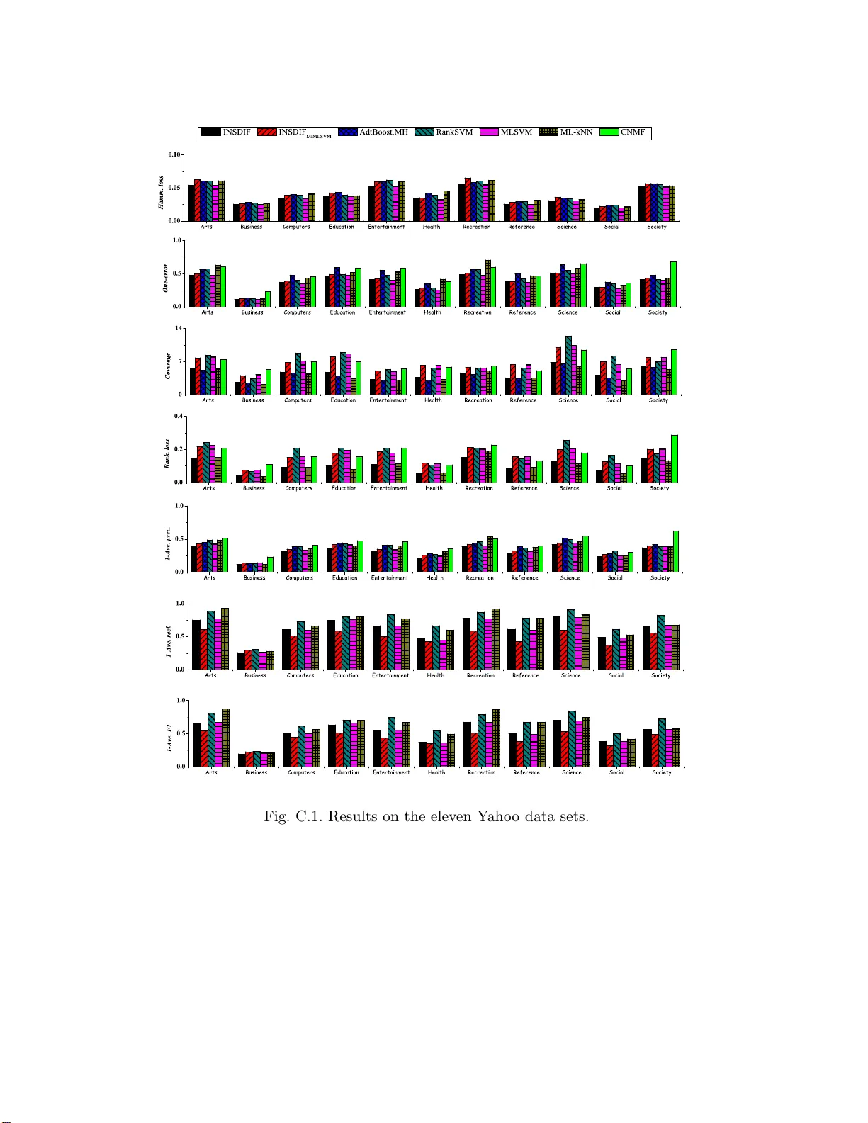
Multi-Inst ance Multi-Lab el Learnin g Zhi-Hua Zhou ∗ , Min-Ling Zhang, Sheng-Jun Huang, Y u-F eng Li National Key L ab or atory for Novel Softwar e T e chnolo gy, Nanjing University, Nanjing 21004 6, China Abstract In this pap er, we pr op ose the MIML ( Mu lti-Instanc e Multi-L ab e l le arning ) framew ork where an example is describ ed b y multiple instances and asso ciated with multiple class lab els. Compared to traditional learning framew orks, the MIML framework is more con- v enien t and n atural for represent ing complicated ob jects wh ic h h a ve multiple seman tic meanings. T o learn from MIML examp les, we prop ose the MimlBoost and MimlSvm algorithms based on a simple degeneration strategy , and exp eriments sh o w that solving problems inv olving complicated ob jects with m ultiple semanti c m eanings in the MIML framew ork ca n lea d to go o d p erforman ce. Considerin g that the degeneration pr o cess ma y lose information, we prop ose the D-MimlSvm algorithm which tac kles MIML p roblems directly in a r egularization framework. Moreo ver, w e sho w that ev en wh en we d o not ha v e access to the r eal ob jects and thus cann ot capture more information from real ob- jects by using the MIML repr esen tatio n, MIML is still usefu l. W e p rop ose the Ins Dif and S ubCod algorithms. InsDif w orks by tr an s forming sin gle-instances in to the MIML represent ation for learning, wh ile SubCod works b y transforming single-lab el examples in to the MIML r epresen tation for learning. Exp eriments sh o w that in some tasks they are able to ac hiev e b etter p erformance than learning the sin gle-instances or single-lab el examples directly . Key wor ds: Mac hin e Learning, Multi-Instance Multi-Lab el Learning, MIML, Multi-Lab el Learning, Multi-Instance Learning ∗ Corresp ond ing author. E-mail: zhouzh@lamda.nju.edu .cn 1 In tro duction In tr aditiona l sup ervise d le arnin g , an ob ject is represen ted b y an instance, i.e., a feature v ector, and asso ciated with a c lass lab el. F ormally , let X denote the instance space (or feature space) and Y the set of class lab els. The task is to lear n a function f : X → Y from a giv en data set { ( x 1 , y 1 ) , ( x 2 , y 2 ) , · · · , ( x m , y m ) } , where x i ∈ X is an instance and y i ∈ Y is the kno wn lab el of x i . Although this formalization is prev ailing and successful, there are many real-world problems whic h do not ﬁt in this framew ork w ell. In particular, each ob ject in this fr a mew ork b elong s to only one concept and therefore the corresp onding instance is ass o ciated w ith a single class lab el. How ev er, man y real-w orld o b jects are complicated, whic h may b elong to multiple concepts sim ultaneously . F or example, an image can b elong to sev eral classes sim ulta neously , e.g., gr asslands , lions , Afric a , etc.; a text do cumen t can b e classiﬁed to sev eral categories if it is view ed f rom diﬀerent asp ects, e.g., scientiﬁc novel , Jules V erne’ s writing or ev en b o oks on tr aveling ; a w eb pag e can b e recognized as news p age , sp o rts p age , so c c er p age , etc. In a sp eciﬁc real task, ma yb e only o ne of the m ultiple concepts is the righ t seman tic meaning. F or example, in image retriev al when a user is in terested in an image with lions, s/he may b e only in terested in the concept lions instead of the other concepts gr assla n ds and Afric a asso ciated with that imag e. The diﬃcult y here is c aused b y those ob jects that in v olve m ultiple concepts. T o c ho ose the rig h t seman tic meaning for suc h ob jects for a sp eciﬁc scenario is the fundamental diﬃcult y of many tasks. In contrast to starting from a large unive rse of all p ossible concepts in v o lv ed in the task, it may b e helpful t o get the subset o f concepts asso ciated with the concerned ob ject at ﬁrst, and then mak e a choice in the small subset later. Ho w eve r, g etting the subset of concepts, that is, assigning pro p er class lab els to suc h ob jects, is still a c hallenging task. W e notice that as an alternat ive to represen ting an ob ject b y a single instance, in man y cases it is p ossible to represen t a complicated ob ject using a set of instances. F or example, m ultiple pa t c hes can b e extracted from an image where eac h patch is described by an instance, and th us the image can b e represen ted b y a set of instances; multiple sections can b e extracted from a do cumen t where eac h section is described by an instance, and th us t he do cumen t can b e represen ted by a set of instances; m ultiple links can b e extracted from a we b page where eac h link is described b y an instance, and th us the w eb page can b e represen ted b y a set of instances. Using multiple instances to represen t t ho se complicated ob jects may b e helpful b ecause some inheren t patterns which are closely related to some lab els ma y b ecome explicit a nd clearer. In this pap er, w e prop ose the MIML ( Multi-Instanc e Multi-L a b el le arni n g ) framew o rk, where an example is described b y m ultiple in- stances and asso ciated with m ultiple class lab els. Compared t o traditional learning fra mew orks, the MIML fr amew or k is more con v e- nien t and natural for represen ting complicated ob jects. T o exploit the adv antages of the MIML represen tation, new learning alg orithms are needed. W e pro p ose the MimlBoost alg o rithm and the MimlSvm algorithm based on a simple degener- ation strategy , and exp erimen ts show that solving pro blems inv olving complicated ob jects with multiple seman tic meanings under the MIML framew ork can lead to go o d p erformance. Considering that the degeneration pro cess ma y lose informa- tion, w e a lso prop ose the D-MimlSvm (i.e., Direct M imlSvm ) algorithm whic h tac kles MIML problems directly in a regula r izat io n framew ork. Exp erimen ts sho w that this “direct” algorithm outp erfor ms the “indirect” M imlSvm algo rithm. In some practical tasks we do not ha v e access to the real ob jects themselv es suc h as the real images and the real we b pa g es; instead, we are giv en o bserv atio na l data where eac h real ob ject has already b een represen ted by a single instance. Th us, in suc h cases w e cannot capture more infor ma t io n from the real o b jects using the MIML represen tation. Ev en in this situation, how ev er, MIML is still useful. W e prop ose the InsDif (i.e., INStance DIFferentiation) alg o rithm whic h transforms single-instances in to MIML examples for learning. This algor it hm is able to ac hiev e a b etter p erformance than learning the single-instances directly in some tasks. This is not stra ng e b ecause for an ob ject asso ciated with m ultiple class lab els, if it is described b y only a single instance, the inf o rmation corresp onding to these lab els are mixed and th us diﬃcult for learning; if w e can transform the single-instance in to a set o f instances in some prop er w a ys, the mixed information migh t b e detac hed to some exten t and th us less diﬃcult for learning. MIML can also b e helpful f or lear ning single-lab el ob jects. W e prop ose the SubCod (i.e., SUB-COncept Disco v ery) algorithm whic h w orks b y disco v ering sub-concepts of the tar g et concept at ﬁrst and then tra nsfor ming the data into MIML examples for learning. This algorithm is a ble to achie v e a b etter p erformance than learning the single-lab el examples directly in some tasks. This is also not strange b ecause for a lab el corresp onding to a high-level complicated concept, it may b e quite diﬃcult to learn this concept directly since ma ny diﬀeren t low er-lev el concepts ar e mixed; if w e can tr ansform t he single-lab el into a set of lab els corresp onding to some sub- concepts, whic h are relativ ely clearer and easier for learning, w e can learn these lab els a t ﬁrst and then deriv e the high- level complicated lab el based on them with a less diﬃculty . The rest of this pap er is orga nized as follow s. In Section 2, w e review some related w ork. In Section 3, we prop ose the MIML f r a mew ork. In Section 4 w e prop ose the MimlBoost and MimlSvm algorithms, and apply them to tasks where the ob jects are represen ted as MIML examples . In Section 5 w e presen t the D-M imlSvm algorithm a nd compare it with the “indirect” M imlSvm algorithm. In Sections 6 and 7, w e study the usefulness of MIML when we do not hav e access to real ob jects. Concretely , in Section 6, we prop ose the InsDif algo rithm and show that using MIML can b e b etter than learning single-instances directly; in Section 7 we prop ose the SubCod alg orithm and show that using MIML can b e b etter than learning single-lab el examples directly . Finally , w e conclude the pap er in Section 8. 2 Related W ork Muc h work has b een dev oted to t he learning of m ulti-lab el examples under the um brella of multi-lab el le arning . Note that m ulti-lab el learning studies the problem where a real-world ob ject described b y one instance is a sso ciated with a n um b er of class lab els 1 , whic h is diﬀerent f rom multi-class learning or m ulti- task learning [28]. In m ulti-class learning eac h ob ject is only asso ciated with a single lab el; while in m ulti-task learning diﬀeren t tasks ma y inv olv e diﬀeren t domains and diﬀeren t data sets. Actually , traditional t w o-class and multi-class problems can b oth b e cast in to m ulti-lab el problems by restricting that each instance has only one lab el. The generalit y of m ulti-lab el problems, ho w ev er, inevitably mak es it more diﬃcult to 1 Most w ork on multi-la b el learning assum es that an ins tance can b e asso ciated with m ultiple v alid lab els, bu t there is also some work assum ing that only one of the lab els among those asso ciated with an in stance is correct [35]. address. One famous approac h to solving m ulti-lab el problems is Sch apire a nd Singer’s Ad aBoost.MH [56], whic h is an extension of AdaBoo st and is the core of a success ful multi-label learning system BoosTexter [5 6]. This approach main tains a set of we igh ts o v er b oth training examples and their lab els in the training phase, where training examples and their corresp onding labels that a r e hard (easy) t o predict get incremen tally higher ( low er) w eigh ts. La t er, De Comit ´ e et al. [22] used alternating decision trees [30] whic h ar e more p ow erful than decision stumps used in BoosTexter to handle multi-lab el data and thus obtained the AdtBoost.MH algorithm. Probabilistic generativ e mo dels ha v e b een f ound useful in m ult i- lab el learning. McCallum [47] prop osed a Bay esian a ppro ac h for m ulti-lab el do cumen t classiﬁcation, where a mixture probabilistic mo del (one mixture comp onen t p er category) is assumed to generate each do cumen t a nd an EM a lgorithm is employ ed to learn the mixture w eigh t s and the w o rd distributions in each mixture component. Ueda and Saito [65] presen ted another generativ e approac h, whic h assumes that the m ulti-lab el text has a mixture of c haracteristic w ords app earing in single-lab el text b elonging t o eac h of the multi-lab els. It is noteworth y that the generativ e mo dels used in [47] a nd [65] are b oth based on learning text frequencies in do cumen ts, and are th us sp eciﬁc to text a pplications. Man y other multi-label learning algor ithms hav e b een dev elop ed, suc h as decision trees, neural net w orks, k -nearest neighbor classiﬁers, suppo rt v ector mac hines, etc. Clare and King [21] dev elop ed a m ulti-lab el v ersion o f C4.5 decision trees through mo difying the deﬁnition of en trop y . Zhang and Zhou [79] presen ted m ulti-lab el neural netw ork Bp-Mll , whic h is derive d from the Ba ckpropagation algorithm by emplo ying an error function to capture the fact that the lab els b elonging to an instance should b e ra nk ed higher than those not b elonging to that instance. Zhang and Zhou [80] also prop osed the M l- k nn algorithm, whic h iden tiﬁes the k near- est neighbors of the concerned instance and then assigns lab els according to the maxim um a p osteriori principle. Elisseeﬀ and W eston [27] prop osed the RankSvm algorithm for multi-lab el learning b y deﬁning a sp eciﬁc cost f unction a nd t he cor- resp onding marg in for m ulti-lab el mo dels. Other kinds of m ulti-lab el Svm s hav e b een dev eloped b y Boutell et al. [11] and G o db ole a nd Saraw agi [33]. In partic- ular, b y hierarc hically approx imating the Bay es optimal classiﬁer for the H-loss, Cesa-Bianc hi et al. [15] prop osed an algorithm whic h outp erfo r ms simple hierar- c hical Svm s. Recen tly , non-negativ e ma t r ix factorization has also b een applied to m ulti-lab el learning [43], and m ulti- lab el dimensionalit y reduction metho ds hav e b een dev elop ed [74, 85]. Roughly sp eaking, earlier a pproac hes to m ulti- lab el learning a t t empt to divide m ulti-lab el learning to a num b er of tw o-class classiﬁcation problems [36, 72] o r transform it in to a lab el ranking problem [27, 56], while some la ter approaches try to exploit the correlation b et w een the lab els [43, 65, 85]. Most studies on m ulti-lab el learning fo cus on text categorization [22, 33, 3 9, 47, 56, 65, 74], and sev eral studies aim to improv e the p erfor ma nce of t ext categorization systems by exploiting additional information given b y the hierarchic al structure of classes [14, 15 , 53] or unlab eled data [43]. In addition to text categorization, m ulti-lab el learning has also b een found useful in many other tasks suc h as scene classiﬁcation [11 ], image and video a nno t a tion [38, 48], bioinformatics [7, 12, 13, 21, 27], a nd even asso ciation rule mining [5 0 , 63]. There is a lot of researc h on multi-instanc e le a rn ing , whic h studies the problem where a real-w orld ob ject describ ed b y a num b er of instances is a sso ciat ed with a single class lab el. Here the training set is comp o sed of many b ags each containing m ultiple instances; a bag is lab eled p ositiv ely if it con tains at least one p ositiv e instance and negatively otherwise. The goal is to lab el unseen bags cor r ectly . Note that although the t r a ining bags are lab eled, the lab els of t heir instances are un- kno wn. This learning framew ork w as formalized by Dietterich et al. [2 4 ] when they w ere inv estigating drug activit y prediction. Long and T an [44] studied the P ac -learnabilit y of m ulti-instance learning and sho w ed that if the instances in the bags are indep enden tly dra wn from pro duct distribution, t he Apr (Axis-P arallel Rectangle) prop osed b y D ietteric h et al. [24] is P ac -learnable. Auer et al. [5 ] show ed that if the instances in the bags are not indep enden t then Apr learning under the m ulti-instance lear ning f r amew or k is NP-hard. Moreo v er, they presen ted a theoretical a lgorithm that do es not require pro duct distribution, which w as transformed in to a practical algorithm named Mul tinst [4]. Blum and Kalai [10] describ ed a reduction from P ac -learning un- der the multi-instance learning framew ork to P ac -learning with one-sided random classiﬁcation noise. They also presen ted an algorithm with smaller sample com- plexit y than that of the algor it hm of Auer et al. [5 ]. Man y m ulti- instance learning algorit hms hav e b een dev elop ed during the past decade. T o name a few, D iverse De nsity [4 5] and Em-dd [83], k - nearest neigh- b or alg o rithms Cit a tion- k nn and Ba yesian- k nn [67], decision tree algo r it hms Relic [54] and Miti [9], neural net w ork algo rithms Bp- mip and extensions [77, 90] and Rbf-mip [7 8 ], rule learning alg orithm Ripper- mi [20], supp ort vec tor ma- c hines and k ernel metho ds mi-Svm and Mi-Svm [3], D d-Svm [18], M issSvm [88], Mi-Kernel [32], Bag-Inst ance Kernel [19], Marginalized M i-Kernel [42 ] and conv ex-h ull metho d Ch-Fd [31], ensem ble algorithms M i-Ensemble [91], Mi- Boosting [70] and MilBoosting [6 ], logistic regression algorithm Mi-lr [51], etc. Actually almost all p opular machine learning algorithms hav e their m ulti- instance vers ions. Most algorithms a ttempt to adapt single-instance sup ervised learning algorithms to the m ulti-instance represen tation, b y shifting their fo cus from discrimination on instances to discrimination on bags [91]. R ecen tly there is some pro p osal on a dapting the m ulti- instance represen tation to single-instance algorithms b y represen tation transformation [93]. It is w orth mentioning that standard multi-instance learning [24] a ssumes that if a bag contains a p ositiv e instance then the bag is p ositiv e; this implies that there exists a key instanc e in a p ositiv e bag. Man y alg orithms w ere designed based o n this assumption. F or example, the p oin t with maximal divers e densit y iden tiﬁed b y the Diverse D ensity a lg orithm [45] actually corresp onds to a k ey instance; man y Svm algorithms deﬁned the margin of a p ositiv e bag b y the marg in of its most p ositiv e instance [3, 19]. As the researc h of m ulti- instance learning go es on, how ev er, some other assumptions ha v e b een introduced [29]. F or example, in contrast to assuming that there is a k ey instance, some w ork has assumed that t here is no k ey instance and ev ery instance con tributes to the bag lab el [17 , 70 ]. There is also a n argumen t that the instances in the bag s should not b e treated indep enden tly [88]. All those assumptions hav e b een put under the um brella of multi-instance learning, and generally , in tac kling real t asks it is diﬃcult to know whic h assumption is the ﬁttest. In other w ords, in diﬀeren t ta sks m ulti-instance learning algorithms based on diﬀeren t assumptions ma y hav e diﬀeren t sup eriorities. In the early y ears of the researc h of multi-instance learning, most w ork considered m ulti-instance classiﬁcation with discrete-v alued outputs. Later, m ulti-instance re- gression with real-v alued outputs was studied [2, 5 2], and diﬀeren t v ersions of gen- eralized mu lti-instance learning ha v e b een deﬁned [58, 6 8]. The main diﬀerence b et w een standard multi-instance learning and generalized m ulti-instance learning is that in standard m ulti-instance learning there is a single concept, and a ba g is p ositiv e if it has a n instance satisfying this concept; while in generalized multi- instance learning [58, 68] there are m ultiple concepts, a nd a bag is p ositiv e o nly when all concepts are satisﬁed (i.e., the bag contains instances from ev ery concept). Recen tly , researc h on multi-instance clustering [82], multi-instance semi-sup ervised learning [49] and m ulti-instance activ e learning [60] ha v e also b een rep orted. Multi-instance learning has also attracted the atten tion of the Ilp communit y . It has b een suggested that multi-instance pro blems could b e regarded as a bias o n inductiv e logic progra mming, and the m ulti-instance paradigm could b e the k ey b e- t w een the pro p ositional a nd relational represen tations, b eing mor e expressiv e than the former, a nd m uc h easier to learn than the latt er [23]. Alphonse and Mat win [1] appro ximated a relational learning problem b y a multi-instance problem, fed t he resulting data to feature selection techniq ues adapted fro m prop ositional r epresen- tations, and then transformed the ﬁltered data back to relational represen tation for a relational learner. Thus , the expressiv e p o w er o f relational represen tation a nd the ease of feature selection o n prop ositional represen ta tion are gracefully com bined. This w ork conﬁrms that m ulti-instance learning can really act as a bridge b etw een prop ositional and relational learning. Multi-instance learning tec hniques ha v e already b een applied to div erse applica- tions including image categorization [17, 18], image retriev a l [71, 84 ], text catego- rization [3, 60], web mining [86], spam detection [37], computer securit y [54], face detection [66, 7 6 ], computer-aided medical diag nosis [31 ], etc. 3 The MIML F ramew ork Let X denote the instance space and Y the set of class lab els. Then, formally , the MIML task is deﬁned as: (a) T raditional sup ervised learning (b) Mu lti-instance learning (c) Multi-label learning (d) Mu lti-instance m ulti-lab el learning Fig. 1. F our d iﬀerent learnin g framew orks • MIML (m ulti-instance multi-label learning): T o learn a function f : 2 X → 2 Y from a giv en data set { ( X 1 , Y 1 ) , ( X 2 , Y 2 ) , · · · , ( X m , Y m ) } , where X i ⊆ X is a set of instances { x i 1 , x i 2 , · · · , x i,n i } , x ij ∈ X ( j = 1 , 2 , · · · , n i ), a nd Y i ⊆ Y is a set o f lab els { y i 1 , y i 2 , · · · , y i,l i } , y ik ∈ Y ( k = 1 , 2 , · · · , l i ). Here n i denotes the n um b er of instances in X i and l i the num b er of lab els in Y i . It is inte resting to compare MIML with the existing fra meworks of tr a ditional sup ervised learning, m ulti-instance learning, and multi-lab el learning. • T raditional sup ervised learning (single-instance single-lab el learning): T o learn a function f : X → Y from a giv en data set { ( x 1 , y 1 ) , ( x 2 , y 2 ) , · · · , ( x m , y m ) } , where x i ∈ X is an instance a nd y i ∈ Y is the know n lab el of x i . • Multi-instance learning (m ulti-instance single-lab el learning): T o learn a func- tion f : 2 X → Y fr o m a given data set { ( X 1 , y 1 ) , ( X 2 , y 2 ) , · · · , ( X m , y m ) } , where X i ⊆ X is a set of instances { x i 1 , x i 2 , · · · , x i,n i } , x ij ∈ X ( j = 1 , 2 , · · · , n i ), and y i ∈ Y is the lab el of X i . 2 Here n i denotes the n um b er of instances in X i . 2 According to notions used in multi-instance learnin g, ( X i , y i ) is a lab eled b ag while X i an unlab eled bag. • Multi-lab el learning (single-instance multi-label learning ) : T o learn a function f : X → 2 Y from a giv en data set { ( x 1 , Y 1 ) , ( x 2 , Y 2 ) , · · · , ( x m , Y m ) } , where x i ∈ X is an instance and Y i ⊆ Y is a set of lab els { y i 1 , y i 2 , · · · , y i,l i } , y ik ∈ Y ( k = 1 , 2 , · · · , l i ). Here l i denotes the n um b er of la b els in Y i . F rom Fig. 1 we can see the diﬀerences among these lear ning framew o rks. In f act, the multi- learning f r a mew orks are resulted fro m the ambiguities in r epresen ting real-w orld ob jects. Multi-instance learning studies the am biguit y in the input space (or instance space), where an o b ject has man y alternative input descriptions, i.e., instances; multi-lab el learning studies the ambiguit y in the output space (or lab el space), where a n ob ject has many alternative output descriptions, i.e., lab els; while MIML considers the am biguities in b oth the input and output spaces sim ultane- ously . In solving real-w orld problems, ha ving a go o d represen tation is often more imp ortant than ha ving a strong learning algorithm, b ecause a go o d represen ta- tion may capture more meaningful information and make the learning task easier to tac kle. Since man y real ob jects are inherited with input am biguit y as w ell as output am biguit y , MIML is more natural and conv enien t fo r tasks in v olving suc h ob jects. It is worth men tioning that MIML is more reasonable than (single-instance) m ulti- lab el learning in many cases. Supp ose a multi-lab el ob ject is describ ed b y one instance but a sso ciat ed with l num b er of class lab els, na mely lab el 1 , lab el 2 , . . . , lab el l . If w e represen t the multi-lab el ob ject using a set of n instances, namely instance 1 , instance 2 , . . . , instance n , the underlying information in a single instance ma y b ecome easier to exploit, a nd for each lab el the n um b er of t r aining instances can b e signiﬁcan tly increased. So , transforming m ulti-lab el examples to MIML examples for learning ma y b e b eneﬁcial in some tasks, whic h will b e sho wn in Sec- tion 6. Moreo v er, when represen ting the m ulti-lab el ob ject using a set of instances, the relation b et w een the input patterns and the seman tic meanings may b ecome more easily disco v erable. Note that in some cases, understanding wh y a particular ob ject has a certain class lab el is ev en more imp o rtan t than simply making an accurate prediction, while MIML oﬀers a p ossibilit y for this purp ose. F or exam- ple, under the MIML represen tatio n, w e ma y discov er that one o b ject has la b el 1 b ecause it con tains instance n ; it has lab el l b ecause it con tains instance i ; while the o ccurrence of b oth instance 1 and instance i triggers lab el j . (a) Afric a is a complicated high-lev el concept (b) T he concept Afric a ma y b ecome easier to learn through exploiting some sub-concepts Fig. 2. MIML can b e helpfu l in learning single-lab el examples inv olving complicated high-lev el concepts MIML can also b e helpful f or learning single-lab el examples inv olving complicated high-lev el concepts. F or example, as F ig. 2(a) sho ws, the concept Afric a has a broad connotation and the images b elonging to Afric a hav e gr eat v ariance, thus it is not easy to classify the top-left image in F ig. 2(a) in to the Afric a class correctly . Ho w ev er, if w e can exploit some low-lev el sub-concepts that are less ambiguous and easier to learn, suc h as tr e e , lions , ele p hant and gr assland sho wn in Fig. 2(b), it is p ossible to induce the concept Afric a m uc h easier than learning the concept Afric a directly . The usefulness of MIML in this pr o cess will b e sho wn in Section 7. Fig. 3. The tw o general degeneration solutions. 4 Solving MIML Problems by Degeneration It is eviden t that traditional sup ervised learning is a degenerated v ersion of mu lti- instance learning as w ell as a degenerated v ersion of mu lti-lab el learning, while traditional sup ervised learning, mu lti-instance learning and multi-lab el learning are all degenerated v ersions of MIML. So, a simple idea to ta c kle MIML is to iden t if y its equiv alence in the traditional sup ervised learning framew ork, using m ulti-instance learning or m ulti-lab el learning as the bridge, as sho wn in Fig. 3. • Solution A : Using mu lti-instance learning as the bridge: The MIML learning task, i.e., to learn a function f : 2 X → 2 Y , can b e transformed into a m ulti-instance learning task, i.e., to learn a function f M I L : 2 X × Y → {− 1 , +1 } . F or any y ∈ Y , f M I L ( X i , y ) = + 1 if y ∈ Y i and − 1 otherwise. The prop er lab els for a new example X ∗ can b e determined accord- ing to Y ∗ = { y | sig n [ f M I L ( X ∗ , y )] = + 1 } . This multi-instance learning task can b e further transformed into a tr aditional sup ervised learning t a sk, i.e., to learn a function f S I S L : X × Y → {− 1 , +1 } , under a constrain t sp ecifying ho w to derive f M I L ( X i , y ) from f S I S L ( x ij , y ) ( j = 1 , 2 , · · · , n i ). F or a ny y ∈ Y , f S I S L ( x ij , y ) = +1 if y ∈ Y i and − 1 otherwise. Here the constrain t can b e f M I L ( X i , y ) = sig n [ P n i j =1 f S I S L ( x ij , y )] whic h has b een used b y Xu a nd F rank [70] in transforming multi-instance learning tasks in to tra ditional sup ervised learning tasks. Note that other kinds of constraint can also b e used here. • Solution B : Using mu lti-lab el learning a s the bridge: The MIML learning t a sk, i.e., to learn a function f : 2 X → 2 Y , can b e trans- formed into a multi-lab el learning task, i.e., to learn a function f M LL : Z → 2 Y . F or an y z i ∈ Z , f M LL ( z i ) = f M I M L ( X i ) if z i = φ ( X i ), φ : 2 X → Z . The prop er lab els for a new example X ∗ can b e determined a ccording to Y ∗ = f M LL ( φ ( X ∗ )). This mu lti-lab el learning ta sk can b e further tr a nsformed into a traditional su- p ervised learning task, i.e., to learn a function f S I S L : Z × Y → {− 1 , +1 } . F or an y y ∈ Y , f S I S L ( z i , y ) = +1 if y ∈ Y i and − 1 otherwise. That is, f M LL ( z i ) = { y | f S I S L ( z i , y ) = +1 } . Here t he mapping φ can b e implemen ted with c on struc- tive clustering whic h w as prop osed by Zhou and Zha ng [9 3 ] in transforming m ulti-instance bags in to traditional single-instances. Note that other kinds of mappings can a lso b e used here. In the rest of this section w e will prop ose t w o MIML algorithms, MimlBoost and MimlSvm . MimlBoost is an illustration of Solution A, which uses c ate gory- wise d e c omp osition f o r the A1 step in Fig. 3 and MiBoosting for A2; MimlSvm is an illustration of Solution B, whic h uses clustering-b a s e d r epr esentation tr ans - formation for t he B1 step and M lSvm for B2. Other MIML algo rithms can b e dev elop ed by taking alternative options. Both MimlBoost a nd MimlSvm are quite simple. W e will see that for dealing with complicated ob jects with m ultiple seman tic meanings, go o d p erformance can b e obtained under the MIML framework ev en by using such simple algor it hms. This demonstrates that the MIML frame- w ork is very promising, a nd w e exp ect b etter p erformance can b e ac hiev ed in t he future if researc hers put fo rw ard more p o werful MIML algo r it hms. 4.1 MimlBoost No w w e prop ose the M imlBoost algorithm according to the ﬁrst solution men- tioned ab ov e, that is, iden tif ying the equiv a lence in the traditional sup ervised learn- ing framew ork using multi-instance learning as the bridge. Note t ha t this strategy can also b e used t o deriv e other kinds of MIML alg o rithms. Giv en an y set Ω, let | Ω | denote its size, i.e., the num b er of elemen ts in Ω; giv en an y predicate π , let [ [ π ] ] b e 1 if π holds and 0 ot herwise; give n ( X i , Y i ), for an y y ∈ Y , let Ψ( X i , y ) = + 1 if y ∈ Y i and − 1 otherwise, where Ψ is a function Ψ : 2 X × Y → {− 1 , +1 } whic h judges whether a lab el y is a prop er lab el of X i or not. The basic assumption of MimlBoost is tha t the lab els are indep enden t so that t he MIML task can b e decomp osed into a series o f m ulti- instance learning tasks to solv e, by treating each lab el a s a t a sk. The pseudo-co de of M imlBoost is summarized in App endix A (T able A.1). In the ﬁrst step of MimlBoost , eac h MIML example ( X u , Y u ) ( u = 1 , 2 , · · · , m ) is transformed into a set of |Y | n umber of m ulti-instance bags, i.e., { [( X u , y 1 ) , Ψ( X u , y 1 )] , [( X u , y 2 ) , Ψ( X u , y 2 )] , · · · , [( X u , y |Y | ) , Ψ( X u , y |Y | )] } . Note that [( X u , y v ) , Ψ( X u , y v )] ( v = 1 , 2 , · · · , |Y | ) is a lab eled m ulti-instance bag where ( X u , y v ) is a bag con- taining n u n um b er of instances, i.e., { ( x u 1 , y v ) , ( x u 2 , y v ) , · · · , ( x u,n u , y v ) } , and Ψ( X u , y v ) ∈ {− 1 , +1 } is the lab el of this bag. Th us, the original MIML data set is transformed in to a m ulti-instance data set con taining m × |Y | nu m b er of bag s. W e order them as [( X 1 , y 1 ) , Ψ( X 1 , y 1 )] , · · · , [( X 1 , y |Y | ) , Ψ( X 1 , y |Y | )] , [( X 2 , y 1 ) , Ψ( X 2 , y 1 )] , · · · , [( X m , y |Y | ) , Ψ( X m , y |Y | )], and let [( X ( i ) , y ( i ) ) , Ψ( X ( i ) , y ( i ) )] denote the i -th of these m × |Y | n um b er of bags whic h con tains n i n um b er of instances. Then, from the data set a m ulti- instance learning function f M I L can b e learned, whic h can accomplish the desired MIML function b ecause f M I M L ( X ∗ ) = { y | sig n [ f M I L ( X ∗ , y )] = +1 } . In this pap er, the MiBoost ing algorithm [70] is used to implemen t f M I L . Note that b y using MiBoosting , the MimlBoost algorithm assumes that all instances in a ba g con tribute indep enden tly in a n equal wa y to the la b el of that bag . F or con v enience, let ( B , g ) denote the bag [( X , y ) , Ψ( X , y )], B ∈ B , g ∈ G , and E denotes the exp ectation. Then, here the g oal is to learn a function F ( B ) minimizing the bag- lev el exp onen tial loss E B E G | B [exp( − g F ( B ))], whic h ultimately estimates the bag-lev el lo g-o dds function 1 2 log P r ( g =1 | B ) P r ( g = − 1 | B ) on the tr a ining set. In eac h b o osting round, t he aim is to expand F ( B ) in to F ( B ) + cf ( B ), i.e., adding a new w eak classiﬁer, so tha t t he exp onen tial loss is minimized. Assuming that all instances in a bag con tribute equally a nd indep enden tly to the bag’s lab el, f ( B ) = 1 n B P j h ( b j ) can b e deriv ed, where h ( b j ) ∈ {− 1 , +1 } is the prediction of the instance-lev el classiﬁer h ( · ) for the j -th instance of the bag B , and n B is the n umber o f instances in B . It has b een sho wn b y [7 0 ] that the b est f ( B ) to b e added can b e a c hiev ed b y seek- ing h ( · ) whic h maximizes P i P n i j =1 [ 1 n i W ( i ) g ( i ) h ( b ( i ) j )], giv en the bag- lev el w eigh ts W = exp( − g F ( B )). By assigning eac h instance the lab el of its bag and the corre- sp onding w eigh t W ( i ) /n i , h ( · ) can b e learned by minimizing the w eigh ted instance- lev el classiﬁcation error. This actually cor r esp onds to the Step 3 a of M imlBoost . When f ( B ) is found, the b est multiplier c > 0 can b e g ot by dir ectly optimizing the exp o nential loss: E B E G | B [exp( − g F ( B ) + c ( − g f ( B )))] = X i W ( i ) exp   c   − g ( i ) P j h ( b ( i ) j ) n i     = X i W ( i ) exp[(2 e ( i ) − 1) c ] , (1) where e ( i ) = 1 n i P j [ [( h ( b ( i ) j ) 6 = g ( i ) )] ] (computed in Step 3b) . Minimization of this ex- p ectation actually corresp onds to Step 3d, where n umeric optimization tec hniques suc h as quasi-Newton metho d can b e used. Note that in Step 3c if e ( i ) ≥ 0 . 5, the Bo osting pro cess will stop [89 ]. Finally , the bag-lev el w eigh ts are up dated in Step 3f a ccording t o the additive structure of F ( B ). 4.2 MimlSvm No w w e prop ose the MimlSvm algorithm according to t he second solution men- tioned b efore, tha t is, iden tifying the equiv alence in the traditional sup ervised learning framew ork using mu lti-lab el learning as the bridge. Not e tha t this strat- egy can a lso b e used to deriv e other kinds of MIML algorithms. Again, giv en any set Ω, let | Ω | denote its size, i.e., the num b er o f elemen ts in Ω; giv en ( X i , Y i ) and z i = φ ( X i ) where φ : 2 X → Z , for any y ∈ Y , let Φ( z i , y ) = +1 if y ∈ Y i and − 1 ot herwise, where Φ is a function Φ : Z × Y → {− 1 , +1 } . The basic assumption o f M imlSvm is that the spatial distribution of the bags carries relev a n t information, and info r mation helpful for lab el discrimination can b e disco v ered b y measuring the closeness b et w een each bag and t he represen ta t ive bags identiﬁed through clustering. The pseudo-co de of MimlSvm is summarized in App endix A (T able A.2). In the ﬁrst step of M imlSvm , the X u of eac h MIML example ( X u , Y u ) ( u = 1 , 2 , · · · , m ) is collected and put into a da t a set Γ. Then, in the second step, k - medoids clustering is p erformed o n Γ. Since eac h data item in Γ, i.e. X u , is an unlab eled m ulti-instance bag instead of a single instance, Hausdorﬀ distance [26] is emplo y ed to measure the distance. The Hausdorﬀ distance is a famous metric for measuring the distance b etw een tw o bag s of p oin ts, whic h has often b een used in computer vision tasks; other tec hniques tha t can measure the distance b et w een bags of p oin ts, suc h as the set kernel [32], can also b e used here. In detail, giv en t w o ba g s A = { a 1 , a 2 , · · · , a n A } and B = { b 1 , b 2 , · · · , b n B } , the Hausdorﬀ distance b et w een A and B is deﬁned as d H ( A, B ) = max { max a ∈ A min b ∈ B k a − b k , max b ∈ B min a ∈ A k b − a k} , (2) where k a − b k measures the distance b et w een the instances a and b , whic h takes the f orm of Euclidean distance here. After t he clustering pro cess, the data set Γ is divided into k partitions, whose medoids are M t ( t = 1 , 2 , · · · , k ), resp ectiv ely . With the help of these medoids, the original m ulti-instance example X u is transformed into a k -dimensional nu- merical v ector z u , where the i -th ( i = 1 , 2 , · · · , k ) comp onen t of z u is the dis- tance b et we en X u and M i , that is, d H ( X u , M i ). In other words , z ui enco des some structure information of the data, that is, the relatio nship b et w een X u and t he i -th partitio n of Γ. This pro cess reassem bles the c onstructive clustering pro cess used by Z hou and Z hang [93] in transforming m ulti-instance examples into single- instance examples except that in [93] the clustering is executed at the instance lev el while here it is executed at t he bag leve l. Th us, the o riginal MIML exam- ples ( X u , Y u ) ( u = 1 , 2 , · · · , m ) ha v e b een transformed in to multi-label examples ( z u , Y u ) ( u = 1 , 2 , · · · , m ), which corresp onds to the Step 3 of M imlSvm . Then, from the data set a m ulti-lab el learning function f M LL can b e learned, whic h can accomplish the desired MIML function b ecause f M I M L ( X ∗ ) = f M LL ( z ∗ ). In this pap er, the MlSvm algorithm [11] is used to implemen t f M LL . Concretely , MlSvm decomp oses the m ulti- lab el learning problem into m ultiple indep enden t binary classiﬁcation problems ( o ne p er class), where eac h example asso ciated with the lab el set Y is regarded as a p ositiv e example when building Svm for any class y ∈ Y , while regarded as a negativ e example when building Svm for an y class y / ∈ Y , as sho wn in the Step 4 of M imlSvm . In making predictions, the T- Criterion [11 ] is used, which actually corresp onds to the Step 5 of the MimlSvm algorithm. That is, the test example is lab eled by a ll the class lab els with p ositiv e Svm sc o r es , except that when all the Svm scores are negativ e, the test example is lab eled b y the class lab el whic h is with the top (least negativ e) score. 4.3 Exp eriments 4.3.1 Multi-L ab el Evaluation C ri teria In tr a ditional sup ervised learning where eac h ob ject has only one class lab el, ac- cur acy is often used as the p erfor mance ev alua tion criterion. T ypically , accuracy is deﬁned as the p ercen tage o f test examples tha t are correctly classiﬁed. When learning with complicated ob jects a sso ciated with multiple la b els simultaneous ly , ho w ev er, accuracy b ecomes less meaningful. F or example, if approach A missed one prop er lab el while a pproac h B missed four prop er lab els for a test example ha ving ﬁv e la b els, it is obv ious that A is b etter than B , but the accuracy of A a nd B may b e iden tical b ecause b oth of them incorrectly classiﬁed the test example. Fiv e criteria are often used for ev aluating the p erforma nce of learning with m ulti- lab el examples [56, 92]; they are h a m ming loss , one-err or , c over a ge , r anking los s and aver age pr e cision . Using the same denotation as that in Sections 3 and 4 , g iv en a test set S = { ( X 1 , Y 1 ) , ( X 2 , Y 2 ) , · · · , ( X p , Y p ) } , these ﬁv e criteria are deﬁned as b elo w. Here, h ( X i ) returns a set of prop er lab els o f X i ; h ( X i , y ) returns a real-v alue indicating the conﬁdence for y to b e a prop er lab el of X i ; r ank h ( X i , y ) returns the rank of y deriv ed from h ( X i , y ). • hloss S ( h ) = 1 p P p i =1 1 |Y | | h ( X i )∆ Y i | , where ∆ stands for the symmetric diﬀerence b et w een t w o sets. The hamming loss ev aluates how many times an ob ject- lab el pair is misclassiﬁed, i.e., a prop er lab el is missed or a wrong lab el is pre- dicted. The p erformance is p erfect when hloss S ( h ) = 0; the smaller the v a lue o f hloss S ( h ), the b etter the p erformance of h . • o ne- erro r S ( h ) = 1 p P p i =1 [ [[arg max y ∈Y h ( X i , y )] / ∈ Y i ] ]. The one-err or ev aluates how man y t imes the top- r a nk ed la b el is not a prop er lab el of the ob ject. The p erfor- mance is p erfect when one-erro r S ( h ) = 0; the smaller t he v alue of one- erro r S ( h ), the b etter the p erformance of h . • cov erage S ( h ) = 1 p P p i =1 max y ∈ Y i r ank h ( X i , y ) − 1 . The c over age ev aluat es ho w fa r it is needed, on the av erage, to go down the list of lab els in order to cov er all the pro p er lab els of t he ob ject. It is lo osely related to precision at the lev el of p erfect recall. The smaller the v alue of cov erage S ( h ), the b etter the p erformance of h . • rlo ss S ( h ) = 1 p P p i =1 1 | Y i || Y i | |{ ( y 1 , y 2 ) | h ( X i , y 1 ) ≤ h ( X i , y 2 ) , ( y 1 , y 2 ) ∈ Y i × Y i }| , where Y i denotes the complemen tary set of Y i in Y . The r a nking lo s s ev a lua t es the av erage fraction of lab el pairs that are misordered for the ob ject. The p er- formance is p erfect when rlo ss S ( h ) = 0; the smaller the v alue of rloss S ( h ), the b etter the p erformance of h . • avgprec S ( h ) = 1 p P p i =1 1 | Y i | P y ∈ Y i |{ y ′ | r ank h ( X i ,y ′ ) ≤ rank h ( X i ,y ) , y ′ ∈ Y i }| r ank h ( X i ,y ) . The aver age pr e- cision ev aluates the a v erage fractio n of prop er lab els ra nk ed ab ov e a particular lab el y ∈ Y i . The p erformance is p erfect when a vgprec S ( h ) = 1; the larger the v alue of avgprec S ( h ), the b etter the p erformance of h . In addition to the ab o v e criteria, w e design tw o new multi-lab el criteria, aver ag e r e c a l l and aver age F1 , as b elo w. • avgrecl S ( h ) = 1 p P p i =1 |{ y | r ank h ( X i ,y ) ≤| h ( X i ) | , y ∈ Y i }| | Y i | . The aver age r e c a l l ev alua tes the a v erag e fraction o f prop er la b els that hav e b een predicted. The p erformance is p erfect when av grecl S ( h ) = 1; the larger the v alue of avgrecl S ( h ), the b etter the p erformance of h . • avgF1 S ( h ) = 2 × a vgprec S ( h ) × a vgrecl S ( h ) a vgprec S ( h )+ a vgrecl S ( h ) . The aver age F1 expresse s a tradeoﬀ b e- t w een the aver age pr e c i s i o n and the aver age r e c a l l . The p erfor mance is p erfect when a vgF1 S ( h ) = 1; the larger the v alue of a vgF1 S ( h ), the b etter the p erfor- mance of h . Note t ha t since the ab ov e criteria measure the p erformance from diﬀerent asp ects, it is diﬃcult for one algorithm to o ut p erform another on ev ery one of these criteria. In the followin g w e study the p erfor ma nce o f MIML alg orithms on t w o tasks in- v olving complicated ob jects with multiple semantic meanings. W e will sho w that for suc h tasks, MIML is a go o d choice, and go o d p erforma nce can b e achiev ed ev en b y using simple MIML alg orithms such as MimlBoost a nd MimlSvm . 4.3.2 Sc ene Classiﬁc ation The scene classiﬁcation data set consists of 2,0 00 na t ur a l scene images b elonging to the classes desert , m ountains , se a , sunset a nd tr e e s . Ove r 22% of the images b elong to m ultiple classes sim ultaneously . Each image has already b een represen ted a s a bag o f nine instances generated b y the Sbn metho d [46 ], whic h uses a G aussian ﬁlter to smo oth the image and then subsamples the image to an 8 × 8 matrix of c olor blobs where eac h blob is a 2 × 2 set of pixels within the matrix. An instance corresp onds to t he combination of a single blob with its four neighboring blobs (up, down, left, righ t), whic h is describ ed with 15 features. The ﬁrst three features represen t the mean R, G, B v a lues of the cen t r al blob and the remaining tw elv e features express the diﬀerences in mean color v alues b etw een the cen tral blob and other four neigh bo ring blobs resp ectiv ely . 3 W e ev a luate the p erformance of the MIML algor it hms MimlBoost and M imlSvm . Note that MimlBoost and MimlSvm are merely prop osed to illustrate the tw o general degeneration solutions to MIML problems shown in F ig. 3. W e do not claim that they ar e the b est algorithms that can b e dev elop ed through the degenera- tion paths. There may exist other pro cess es for transforming MIML examples in to m ulti-instance single-lab el (MISL) examples or single-instance multi-label (SIML) examples. Ev en by using the same degeneration pro cess as that used in Miml- Boost and M imlSvm , there are also many alternatives to realize the second step. F or example, by using mi-Svm [3] to replace the MiBoosting used in Miml- Boost and b y using the t w o- lay er neural net w ork structure [81] to replace the MlSvm used in MimlSvm , w e get MimlSvm mi and MimlNn respective ly . Their p erformance is also ev aluated in our exp erimen ts. W e compare the MIML algorithms with sev eral state-of-the-art algorithms for learning with multi-label examples , including AdtBoost.MH [22], RankSvm [27], MlSvm [11] and Ml- k nn [8 0 ]; these algor ithms hav e b een introduced brieﬂy in Section 2. Note that these are single-instance algorithms that regard each image as a 135-dimensional feature v ector, which is obt a ined by concatenating the nine 3 The data set is av ailable at http://la mda.nju.edu.cn/data MIMLimage.ashx. instances in the dir ection from upp er-left to right-bot t om. The parameter conﬁgurations of RankSvm , MlSvm and Ml- k nn a r e set b y con- sidering the strategies adopted in [2 7], [11] and [8 0] respective ly . F or RankSvm , p olynomial k ernel is used where p o lynomial degrees of 2 to 9 a re considered as in [2 7] and c hosen by hold-out tests on training sets. F o r MlSvm , Gaussian k ernel is used. F or M l- k nn , the n um b er of nearest neigh b ors considered is set to 10. The b o osting rounds of AdtBoost.MH a nd M imlBoost are set to 25 and 50, resp ectiv ely; The p erformance of the t w o algo rithms at diﬀerent b o osting rounds is sho wn in App endix B (F ig. B.1) , it can b e observ ed that at tho se rounds the p erformance o f the algorithms hav e b ecome stable. Gaussian k ernel Libsvm [16] is used for the Step 3a of M imlBoost . The M imlSvm and MimlSvm mi are also realized with Gaussian k ernels. The parameter k o f MimlSvm is set to b e 20% of the n um b er o f tra ining imag es; The p erformance o f this alg o rithm with diﬀeren t k v alues is sho wn in App endix B (Fig. B.2), it can b e observ ed that the setting of k do es not signiﬁcan tly a ﬀ ect the p erformance o f MimlSvm . Note that in App endix B (Figs. B.1 and B.2) w e plot 1 − aver age p r e cision , 1 − aver age r e c al l and 1 − aver age F1 suc h that in all the ﬁgures, the low er the curv e, the b etter the p erformance. Here in the exp erimen ts, 1,500 images are used as training examples while the remaining 500 imag es are used for testing. Exp erimen ts are rep eated for thirty runs b y using random training/test partitions, and the av erage and standard deviation are summarized in T able 1, 4 where the b est p erfo r ma nce on eac h criterion has b een highligh ted in b oldface. P airwise t -tests with 95% signiﬁcance lev el disclose that all the MIML algorithms are signiﬁcan tly b etter than AdtBoost.M H and MlSvm o n all the sev en ev al- uation criteria. This is impressiv e since a s men tioned b efore, these ev aluation cri- teria measure the learning p erformance from diﬀeren t asp ects and one algorithm rarely outp erfo r ms another a lg orithm on all criteria. MimlSvm and MimlSvm mi are b oth signiﬁcantly b etter than RankSvm on all the ev aluatio n criteria, while MimlBoost and M imlNn are b o th signiﬁcan tly b etter than RankSvm on the 4 F or the shared implementat ion of Adt Boost.MH (http://www.grappa.univ-lille3.fr/ grappa/en index.php 3?inf o=soft ware), r anking loss , aver age r e c al l and aver age F1 are not a v ailable in the p rogram’s ou tp uts. T able 1 Results (mean ± std.) on scene classiﬁcation data set (‘ ↓ ’ in dicates ‘the smaller the b etter’; ‘ ↑ ’ indicates ‘the larger th e b etter’) Compared Ev aluation Criteria Algorithms hloss ↓ one - er r or ↓ cove r age ↓ r loss ↓ avepr e c ↑ aver ec l ↑ aveF 1 ↑ MimlBoost .193 ± .007 .347 ± .019 .984 ± .0 49 .178 ± .011 .779 ± .012 .433 ± .027 .556 ± .023 MimlSvm 189 ± .009 .354 ± .022 1.087 ± .047 .201 ± .011 .765 ± .013 .556 ± .020 . 644 ± .018 MimlSvm mi .195 ± .008 .317 ± .0 18 1.068 ± .052 .197 ± .011 .783 ± .0 11 .587 ± .019 .671 ± .015 MimlNn .185 ± .0 08 .351 ± .026 1.057 ± .054 .196 ± .013 .771 ± .015 .509 ± .022 . 613 ± .020 AdtBoost.MH .211 ± .006 .436 ± .019 1.223 ± .050 N/A .718 ± .012 N/A N/A RankSvm .210 ± .024 .395 ± .075 1.161 ± .154 .221 ± .040 .746 ± .044 .529 ± .068 . 620 ± .059 MlSvm .232 ± .004 .447 ± .023 1.217 ± .054 .233 ± .012 .712 ± .013 .073 ± .010 . 132 ± .017 Ml- k nn .191 ± .006 .370 ± .017 1.085 ± .048 .203 ± .010 .759 ± .011 .407 ± .026 . 529 ± .023 ﬁrst ﬁv e criteria. MimlNn is signiﬁcantly b etter than Ml- k nn on all the ev al- uation criteria. Both M imlBoost and M imlSvm mi are signiﬁcan tly b etter than Ml- k nn o n all criteria except hammi n g loss . MimlSvm is signiﬁcan tly b etter than Ml- k nn on on e-err or , aver age pr e cision , aver ag e r e c al l and aver ag e F1 , while there are ties on the other criteria. Moreov er, note that the b est p erformance on all ev al- uation criteria are alwa ys at tained by MIML algorithms. O verall, comparison on the scene classiﬁcation ta sk sho ws that the MIML algorithms can b e signiﬁcan tly b etter tha n the non-MIML a lgorithms; this v alidates the p o w erfulness of the MIML framew ork. 4.3.3 T ext Cate gorization The Reuters -21578 data set is used in this exp erimen t. The sev en most frequen t categories are considered. After remov ing do cumen ts that do no t ha v e lab els or main t exts, a nd ra ndo mly remov ing some do cuments that ha v e only one lab el, a data set con taining 2,00 0 do cumen ts is obtained, where o v er 14.9% do cumen ts ha v e m ultiple lab els. Eac h do cumen t is represen ted as a bag of instances a ccording to the metho d used in [3 ]. Brieﬂy , t he instances are obtained b y splitting each do cumen t in to passages using ov erlapping windo ws of maximal 50 w ords eac h. As a result, there are 2,000 bag s and the n um b er of instances in eac h bag v aries from 2 to 2 6 (3.6 on a v erage). The instances are r epresen ted based on term frequency . The w ords with high f requencies are considered, excluding “function words ” that T able 2 Results (mean ± s td.) on text categ orization data set (‘ ↓ ’ indicates ‘the smaller the b etter’; ‘ ↑ ’ indicates ‘the larger th e b etter’) Compared Ev aluation Criteria Algorithms hloss ↓ one - er r or ↓ cove r age ↓ r loss ↓ avepr e c ↑ aver ec l ↑ aveF 1 ↑ MimlBoost .053 ± .004 .094 ± .014 .387 ± .037 .035 ± .005 . 937 ± .008 .792 ± .010 .858 ± .008 MimlSvm .033 ± .0 03 .066 ± .011 .313 ± .035 .023 ± .004 . 956 ± .006 .925 ± .010 .940 ± .008 MimlSvm mi .041 ± .004 .055 ± .0 09 .284 ± .030 .020 ± .00 3 .965 ± .0 05 .921 ± .012 .9 42 ± .007 MimlNn .038 ± .002 .080 ± .010 .320 ± .030 .025 ± .003 . 950 ± .006 .834 ± .011 .888 ± .008 AdtBoost.MH .055 ± .005 .120 ± .017 .409 ± .047 N/A .926 ± .011 N/A N/A RankSvm .120 ± .013 .196 ± .126 .695 ± .466 .085 ± .077 . 868 ± .092 .411 ± .059 .556 ± .068 MlSvm .050 ± .003 .081 ± .011 .329 ± .029 .026 ± .003 . 949 ± .006 .777 ± .016 .854 ± .011 Ml- k nn .049 ± .003 .126 ± .012 .440 ± .035 .045 ± .004 . 920 ± .007 .821 ± .021 .867 ± .013 ha v e b een remo v ed from the v o cabulary using the Smar t stop-list [55]. It has b een found that based on do cumen t frequency , the dimensionalit y of the data set can b e reduced to 1 - 10% without lo ss of eﬀectiv eness [73]. Thus , w e use the to p 2% frequen t w ords, and therefore eac h instance is a 2 4 3-dimensional feature v ector. 5 The parameter conﬁgurations of R ankSvm , MlSvm and M l- k nn are set in t he same wa y as in Section 4.3.2. The b o osting rounds of AdtBoost.MH and Miml- Boost ar e set to 25 and 5 0, resp ectiv ely . Linear kernels are used. The parameter k of MimlSvm is set to b e 20% of the n um b er of training images. The single-instance algorithms regard eac h do cumen t as a 24 3 -dimensional feature v ector whic h is obtained b y a g gregating all the instances in the same bag; this is equiv alen t to represen t the do cumen t using a sole term frequency feature ve ctor. Here in the exp erimen ts, 1,500 do cumen ts are used as training examples while the remaining 500 do cumen ts are used f o r testing. Exp erimen ts are r ep eated for thirt y runs b y using ra ndom training/test partitions, and the av erage and standard deviation are summarized in T able 2, where the b est p erformance on eac h criterion has b een hig hligh ted in b oldface. P airwise t - tests with 95% signiﬁcance lev el disclose that, impressiv ely , b oth M imlSvm and M imlSvm mi are signiﬁcan tly b etter t ha n all the non- MIML algorit hms. MimlNn is signiﬁcantly b etter than AdtBoost.MH , RankSvm , and M l- k nn on all the 5 The data set is av ailable at http://la mda.nju.edu.cn/data MIMLtext.ashx ev a luation criteria; signiﬁcan tly b etter than MlSvm on hamming loss , aver ag e r e c a l l and ave r age F1 while there are t ies on t he other criteria. MimlBoost is signiﬁcan t ly b etter than AdtBoost. MH on all criteria except that there is a tie on hamming loss ; signiﬁcan tly b etter than R ankSvm on all criteria; signiﬁcan tly b etter than MlSvm on aver age r e c a l l and there is a tie on aver age F1 ; signiﬁcan tly b etter than Ml- k nn on one-err or , c over age , r an k ing loss and ave r age pr e cision . Moreo v er, note that the b est p erformance on all ev aluation criteria are alw a ys at- tained by MIML algorithms. Ov erall, comparison o n the text categorization task sho ws that t he MIML a lgorithms are b etter than the non-MIML algorithms; this v alidates the p o w erfulness o f the MIML fr amew or k. 5 Solving MIML Problems by Regularization The degeneration metho ds presen ted in Section 4 ma y lose informa t ion during the degeneration pro cess, and th us a “direct” MIML alg orithm is desirable. In this section w e prop ose a regularization metho d for MIML. In con trast to MimlSvm and MimlSvm mi , this metho d is dev elop ed from the regula r izat io n framew ork directly and so w e call it D-MimlSvm . The basic assumption of D-M imlSvm is that the la b els asso ciated to the same example hav e some relatedness, and the p erformance of classifying the bags dep ends on the loss b etw een the lab els and the predictions on the bags as we ll as on the constituen t instances. Moreo ver, considering that for an y class lab el the n um b er of p ositive examples is smaller than that of negat ive examples, this metho d incorp or a tes a mec hanism to deal with class im balance. W e emplo y the constrained conca v e-conv ex pro cedure ( Cccp ) whic h has w ell-studied con v ergence pro p erties [62] to solv e the resultan t non-conv ex optimization problem. W e also presen t a cutting plane algorit hm that ﬁnds the solution eﬃcien tly . 5.1 The L oss F unction Giv en a set of MIML training examples { ( X 1 , Y 1 ) , ( X 2 , Y 2 ) , · · · , ( X m , Y m ) } , the goal of D -MimlSvm is to learn a mapping f : 2 X → 2 Y where the prop er la b el set f or eac h bag X ⊆ X corr esp onds to f ( X ) ⊆ Y . Sp eciﬁcally , D-MimlSvm c ho oses to instan tiate f with T functions, i.e. f = ( f 1 , f 2 , · · · , f T ), where T is the n um b er o f lab els in the lab el space Y = { l 1 , l 2 , · · · , l T } . Here, the t -th f unction f t : 2 X → R determines the b elong ing ness of l t for X , i.e. f ( X ) = { l t | f t ( X ) > 0 , 1 ≤ t ≤ T } . In addition, eac h single instance x ∈ X in a bag X can b e view ed as a bag { x } con taining only o ne instance, suc h tha t f ( { x } ) = ( f 1 ( { x } ) , f 2 ( { x } ) , · · · , f T ( { x } )) is also a w ell-deﬁned function. F or con v enience, f ( { x } ) and f t ( { x } ) are simpliﬁed as f ( x ) and f t ( x ) in t he rest of this section. T o tr ain the comp onen t functions f t (1 ≤ t ≤ T ) in f , D-MimlSvm employ s the follo wing empirical loss function V inv olving t w o terms (balanced by λ ): V ( { X i } m i =1 , { Y i } m i =1 , f ) = V 1 ( { X i } m i =1 , { Y i } m i =1 , f ) + λ · V 2 ( { X i } m i =1 , f ) (3) Here, the ﬁrst term V 1 considers the loss b et w een the ground-truth lab el set of eac h training ba g X i , i.e. Y i , to its predicted lab el set, i.e. f ( X i ). Let y it = 1 if l t ∈ Y i holds (1 ≤ i ≤ m, 1 ≤ t ≤ T ). Otherwise, y it = − 1. F urthermore, let ( z ) + = max(0 , z ) denote the hinge loss function. Accordingly , the ﬁrst loss term V 1 is deﬁned a s: V 1 ( { X i } m i =1 , { Y i } m i =1 , f ) = 1 mT m X i =1 T X t =1 (1 − y it f t ( X i )) + (4) The second term V 2 considers the loss b etw een f ( X i ) and the predictions of X i ’s constituen t instances, i.e. { f ( x ij ) | 1 ≤ j ≤ n i } , which reﬂects the relation- ships b et w een the bag X i and its instances { x i 1 , x i 2 , · · · , x i,n i } . Here, the com- mon assumption in m ulti-instance learning is tha t the strength fo r X i to ho ld a lab el is equal to the ma ximum strength for its instances to hold the la b el, i.e. f t ( X i ) = max j =1 , ··· ,n i f t ( x ij ). 6 Accordingly , the second loss term V 2 is deﬁned a s: V 2 ( { X i } m i =1 , f ) = 1 mT m X i =1 T X t =1 l  f t ( X i ) , max j =1 , ··· ,n i f t ( x ij )  (5) Here, l ( v 1 , v 2 ) can b e deﬁned in v arious wa ys and is set to b e the l 1 loss in this pap er, i.e. l ( v 1 , v 2 ) = | v 1 − v 2 | . By com bining Eq. 4 and Eq. 5, the empirical loss function V in Eq. 3 is then sp eciﬁed as: 6 Note that this assump tion m a y b e restrictive to some exten t. There are m an y cases where the lab el of the b ag do es not rely on the instance with the maxim u m predictions, as discussed in Section 2. In addition, in classiﬁcation only the sign of prediction is imp ortant [19], i.e. sig n ( f t ( X i )) = sig n ( m ax j =1 , ··· ,n i f t ( x ij )). Ho w ev er , in this p ap er th e ab o v e common assu mption is still adopted due to its p opularit y and simplicit y . V ( { X i } m i =1 , { Y i } m i =1 , f ) = 1 mT m X i =1 T X t =1 (1 − y it f t ( X i )) + + λ mT m X i =1 T X t =1 l  f t ( X i ) , max j =1 , ··· ,n i f t ( x ij )  (6) 5.2 R epr esenter T h e or em fo r MI ML F or simplicit y , w e assume that each function f t is a linear mo del, i.e., f t ( x ) = h w t , φ ( x ) i where φ is the feature map induced by a ke rnel function k a nd h· , ·i de- notes the standard inner pro duct in the Repro ducing Kernel Hilb ert Space (RKHS) H induced by the k ernel k . W e recall tha t a n instance can b e regarded as a bag con taining only one instance, so the k ernel k can b e an y k ernel deﬁned on a set of instances, such as the set kernel [32]. In the case o f classiﬁcation, ob jects (bags or instances) are classiﬁed according to the sign of f t . D-MimlSvm assumes that the lab els asso ciated with a bag should ha v e some re- latedness; o therwise t hey should not b e asso ciated with the bag sim ultaneously . T o reﬂect this basic assumption, D-M imlSvm regularizes the empirical loss function in Eq. 6 with a n additional t erm Ω( f ): Ω( f ) + γ · V ( { X i } m i =1 , { Y i } m i =1 , f ) (7) Here, γ is a regularization parameter bala ncing the mo del complexit y Ω( f ) a nd the empirical risk V . Inspired b y [28], w e a ssume that the relatedness among the lab els can b e measured b y the mean function w 0 , w 0 = 1 T T X t =1 w t (8) The original idea in [28] is to minimize P T t =1 || w t − w 0 || 2 and mean while minimize || w 0 || 2 , i.e. to set the regularizer as: Ω( f ) = 1 T T X t =1 || w t − w 0 || 2 + η || w 0 || 2 (9) According t o Eq.8, the ﬁrst t erm in the R HS of Eq. 9 can b e rewritten as: 1 T T X t =1 k w t − w 0 k 2 = 1 T T X t =1 k w t k 2 − k w 0 k 2 (10) Therefore, b y substituting Eq. 10 in to Eq. 9, the regularizer can b e simpliﬁed as: Ω( f ) = 1 T T X t =1 || w t || 2 + µ || w 0 || 2 (11) F urther note that k w t k 2 = k f t k 2 H and k w 0 k 2 = k P T t =1 f t T k 2 H , b y substituting Eq. 11 in to Eq. 7, we ha v e t he regular izat io n framew ork of D-MimlSvm as fo llows: min f ∈H 1 T T X t =1 k f t k 2 H + µ k P T t =1 f t T k 2 H + γ · V ( { X i } m i =1 , { Y i } m i =1 , f ) (1 2) Here, µ is a parameter t o trade oﬀ the discrepancy and commonness among the lab els, that is, ho w similar o r dissimilar the w t ’s are. Refer to Eq. 10, w e ha v e Ω( f ) = 1 T P T t =1 k f t k 2 H + µ k P T t =1 f t T k 2 H = 1 T P T t =1 k f t − P T t =1 f t T k 2 H + ( µ + 1) k P T t =1 f t T k 2 H . In tuitiv ely , when µ + 1 (or µ ) is large, minimization of Eq. 12 will fo rce k P T t =1 f t T k 2 H to tend to b e zero and the discrepancy among the lab els b ecomes more imp ortan t; when µ + 1 (o r µ ) is small, minimization of Eq. 12 will force k f t − P T t =1 f t T k 2 H to tend to b e zero and the commonness among the lab els b ecomes more imp or t a n t [28]. Giv en the ab ov e setup, w e can prov e the fo llowing represen ter theorem. Theorem 1 The minim i z er of the optimization pr oblem 12 admits an exp a nsion f t ( x ) = m X i =1   α t,i 0 k ( x , X i ) + n i X j =1 α t,ij k ( x , x ij )   wher e al l α t,i 0 , α t,ij ∈ R . Pro of. Analogous to [28], w e ﬁrst in tro duce a com bined feature map Ψ ( x , t ) =    φ ( x ) √ r , 0 , · · · , 0 | {z } t − 1 , φ ( x ) , 0 , · · · , 0 | {z } T − t    and its decision function, i.e., ˆ f ( x , t ) = h ˆ w , Ψ( x , t ) i where ˆ w = ( √ r w 0 , w 1 − w 0 , · · · , w T − w 0 ) . Here r = µT + T . Let ˆ k denote the k ernel function induced b y Ψ and ˆ H is its corresp onding RKHS. W e ha v e Eqs. 13 and 14. ˆ f ( x , t ) = h ˆ w , Ψ( x , t ) i = h ( w 0 + w t − w 0 ) , φ ( x ) i = h w t , φ ( x ) i = f t ( x ) (13) k ˆ f k 2 ˆ H = || ˆ w || 2 = T X i =1 || w t − w 0 || 2 + r || w 0 || 2 = T X i =1 || w t || 2 + µ T || w 0 || 2 (14) Therefore, loss function in Eq.6 can b e represen ted by ˆ V ( { X i } m i =1 , { Y i } m i =1 , ˆ f ), i.e., ˆ V ( { X i } m i =1 , { Y i } m i =1 , ˆ f ) = 1 mT m X i =1 T X t =1  1 − y it ˆ f ( X i , t )  + + λ mT m X i =1 T X t =1 l  ˆ f ( X i , t ) , max j =1 , ··· ,n i ˆ f ( x ij , t )  . (15) Th us, Eq. 12 is equiv a len t to min ˆ f ∈ ˆ H 1 T || ˆ f || 2 ˆ H + γ ˆ V ( { X i } m i =1 , { Y i } m i =1 , ˆ f ) . (16) Note that || ˆ f || 2 ˆ H : [0 , ∞ ) → R is a strictly monotonically increasing function. According to represen ter theorem (Theorem 4.2 in [5 7 ]), eac h minimizer ˆ f o f the functional risk in Eq. 16 admits a represen tation of the form ˆ f ( x , t ) = T X t =1 m X i =1   β t,i 0 ˆ k (( X i , t ) , ( x , t )) + n i X j =1 β t,ij ˆ k (( x ij , t ) , ( x , t ))   , (17) where β t,ij ∈ R a nd t he corresp onding w eigh t v ector ˆ w is represen ted as ˆ w = T X t =1 m X i =1   β t,i 0 Ψ ( X i , t ) + n i X j =1 β t,ij Ψ ( x ij , t )   . (18) Finally , with Eqs. 1 3 and 1 8 , w e hav e f t ( x ) = h w t , φ ( x ) i = h w , Ψ( x , t ) i = m X i =1   α t,i 0 k ( x , X i ) + n i X j =1 α t,ij k ( x , x ij )   (19) where α t,ij = 1 √ r ( P t β t,ij ) + β t,ij /r .  Note that x in Eq. 19 can b e regarded not only as a ba g X i but also an instance x ij . In other words, b o th f t ( X i ) and f t ( x ij ) can b e o btained by Eq. 19. 5.3 Optimization Considering the use of l 1 loss fo r l ( v 1 , v 2 ), Eq.12 can b e re- written as min f ∈H , ξ , δ 1 T T X t =1 k f t k 2 H + µ k P T t =1 f t T k 2 H + γ mT ξ ′ 1 + γ λ mT δ ′ 1 s.t. y it f t ( X i ) ≥ 1 − ξ it , ξ ≥ 0 , − δ it ≤ f t ( X i ) − max j =1 ,...,n i f t ( x ij ) ≤ δ it ∀ i = 1 , . . . , m, t = 1 , . . . , T (20) where ξ = [ ξ 11 , ξ 12 , · · · , ξ it , · · · , ξ mT ] ′ are slac k v ar ia bles for the errors on the tra in- ing bags for eac h lab el, δ = [ δ 11 , δ 12 , · · · , δ it , · · · , δ mT ] ′ , and 0 and 1 are all-zero and all-one v ector, resp ectiv ely . Without loss of generality , assume tha t the bags and instances are ordered as ( X 1 , · · · , X m , x 11 , · · · , x 1 ,n 1 , · · · , x m, 1 , · · · , x m,n m ). Thus , each ob ject (bag or in- stance) in the tra ining set can then b e indexed b y the following function I , i.e.,            I ( X i ) = i I ( x ij ) = m + i − 1 P l =1 n l + j for j = 1 , · · · , n i and i = 1 , · · · , m . With this ordering, w e can obtain the ( m + n ) × ( m + n ) kerne l matrix K deﬁned on all ob jects in the training set, where n = P m i =1 n i . D enote the i -th column of K b y k i . According to theorem 1, w e ha v e f t ( X i ) = k ′ I ( X i ) α t + b t and f t ( x ij ) = k ′ I ( x ij ) α t + b t . Here, the bias b t for each lab el is included. According to deﬁnition of f t in Eq. 19, Eq. 20 can b e cast as the optimization problem min A , ξ , δ , b 1 2 T T X t =1 α ′ t K α t + µ T 2 1 ′ A ′ K A 1 + γ mT ξ ′ 1 + γ λ mT δ ′ 1 (21) s.t. y it ( k ′ I ( X i ) α t + b t ) ≥ 1 − ξ it , ξ ≥ 0 , k ′ I ( x ij ) α t − δ it ≤ k ′ I ( X i ) α t , k ′ I ( X i ) α t − max j =1 , ··· ,n i k ′ I ( x ij ) α t ≤ δ it , where A = [ α 1 , α 2 , · · · , α T ] and b = [ b 1 , b 2 , · · · , b T ] ′ . The ab ov e optimization problem is a non-conv ex optimization problem since the last constrain t is non-conv ex. Note that this non-conv ex constraint is a diﬀerence b et w een tw o con v ex f unctions, and thus the optimization problem can b e solved b y Cccp [1 9 , 62], whic h is one of the most standard tec hniques to solv e suc h kind of non-con v ex optimization problems. Cccp is guaran teed to con verge to a lo cal minim um [75], and in many cases it can ev en con v erge to a global solution [25]. Here, for solving the optimization problem 21 , Cccp w orks b y solving a sequen tial con v ex quadratic problems. Concretely , giv en t he initial subgradien t P n i j =1 ρ ij t k ′ I ( x ij ) α t of ma x j =1 , ··· ,n i k ′ I ( x ij ) α t , w e solv e the follow ing con v ex quadratic optimization (QP) problem min A , ξ , δ , b 1 2 T T X t =1 α ′ t K α t + µ T 2 1 ′ A ′ K A 1 + γ mT ξ ′ 1 + γ λ mT δ ′ 1 (22) s.t. y it ( k ′ I ( X i ) α t + b t ) ≥ 1 − ξ it , ξ ≥ 0 , k ′ I ( x ij ) α t − δ it ≤ k ′ I ( X i ) α t , k ′ I ( X i ) α t − X n i j =1 ρ ij t k ′ I ( x ij ) α t ≤ δ it . Then, in the next itera t io n w e up date ρ ij k according to ρ ij t =            = 0 , if k ′ I ( x ij ) α t 6 = max k =1 , ··· ,n i  k ′ I ( x ik ) α t  , = 1 /n d , o therwise , where n d is the nu m b er of active x ij ’s. It holds n i P j =1 ρ ij t = 1 for any t ’s. The iteration con tin ues and this pro cedure is guaranteed to con v erge to a lo cal minim um. 5.4 Hand ling Cla s s-Imb ala n c e The ab ov e solution may b e impro v ed further if w e explicitly tak e in to accoun t the instance-lev el class-im balance, that is, for any class lab el the n um b er of p ositive instances is smaller than the n um b er of ne gative instances in MIML problems. W e can roughly estimate the i m b alanc e r ate , whic h is the ratio of the num b er o f p ositiv e instances to that of negativ e instances, for eac h class lab el using the strat- egy adopted by [41]. In detail, for a sp eciﬁc lab el y ∈ Y , we can divide the t raining bags { ( X 1 , Y 1 ) , ( X 2 , Y 2 ) , · · · , ( X m , Y m ) } into t w o subsets, A 1 = { ( X i , Y i ) | y ∈ Y i } and A 2 = { ( X i , Y i ) | y / ∈ Y i } . It is obv ious that all the instances in A 2 are negativ e to y . Then, for ev ery ( X i , Y i ) in A 1 , assuming t ha t t he instances of diﬀerent lab els is roughly equally distributed, the n um b er of p o sitiv e instances of y in ( X i , Y i ) is roughly n i × 1 | Y i | where | Y i | returns the num b er of lab els in Y i . Th us, the imbalance rate of y is: ibr ( y ) = m X i =1 y ∈ Y i n i | Y i | × 1 m P i =1 n i = m X i =1 y ∈ Y i n i n × | Y i | . There ar e man y class-im balance learning metho ds [69]. One o f the most p opular and eﬀectiv e metho ds is r esc ali n g [8 7], whic h can b e incorp orated into our f ramew o r k easily . In short, after o btaining the estimated imbalance ra te f or eve ry class lab el, w e can use these rates to mo dulate the loss caused by diﬀeren t misclassiﬁcations. In detail, ξ in Eq. 22 is directly related to the hinge loss (1 − y it f t ( X i )) + . According to the r escaling metho d [87], without loss of g enerality , we can rewrite the loss function in to Eq. 23 .  y it + 1 2 − y it × ibr ( y it )  (1 − y it f t ( X i )) . (23) Let τ = [ τ 11 , τ 12 , · · · , τ it , · · · , τ mT ], where τ it =  y it +1 2 − y it × ibr ( y it )  . Then, t o minimize the loss deﬁned in Eq. 23, Eq. 22 b ecomes Eq. 24. Here ξ ′ τ indicates the w eigh ted lo ss after considering the instance-lev el class-im bala nce. It is eviden t that the pr o blem in Eq. 24 is still a standard QP problem. min A , ξ , δ , b 1 2 T T X t =1 α ′ t K α t + µ T 2 1 ′ A ′ K A 1 + γ mT ξ ′ τ + γ λ mT δ ′ 1 (24) s.t. y it ( k ′ I ( X i ) α t + b t ) ≥ 1 − ξ it , ξ ≥ 0 , k ′ I ( x ij ) α t − δ it ≤ k ′ I ( X i ) α t , k ′ I ( X i ) α t − n i X j =1 ρ ij t k ′ I ( x ij ) α t ≤ δ it . 5.5 Eﬃcient Algorithm Eq. 24 is a large-scale quadratic programming problem that inv olv es man y con- strain ts and v ariables. T o mak e it tra cta ble a nd scalable, and observing that most of the constrain ts in Eq. 24 are redundant, w e presen t a n eﬃcien t algorithm whic h constructs a nested sequence of t ig h ter relaxations of the original problem using the cutting plane metho d [40]. Similar to its use with structured prediction [64], we add a constraint (or a cut) that is most violated by the curren t solution, and then ﬁnd the solution in the up dated feasible region. Suc h a pro cedure will con v erge to an optimal (or ε -sub optimal) solution o f t he origina l pro blem. Moreov er, Eq. 24 supp orts a natural problem decomp osition since its constrain t mat r ix is a blo c k diagonal matrix, i.e., each blo c k corresp onds to one lab el. The pseudo-co de of the alg orithm is summarized in App endix A (T a ble A.3). W e ﬁrst initialize the w orking sets S t ’s as empt y sets and the solutions as all zeros (Line 1). Then, instead of testing a ll the constraints, whic h is rather exp ensiv e when there are lots of constraints , we use the sp eedup heuristic as describ ed in [61], i.e., we use p constrain ts to appro ximate the whole constrain ts (Line 4). Smola and Sc h¨ olk opf [61] hav e shown t ha t when p is larger than 59 , the selected violated constrain t is with probability 0.95 among the 5% most violated constrain ts a mong all constrain t s. The Loss i (Line 5 ) is calculated a s max { 0 , u ′ x − d } where u and d are the linear co eﬃcien ts and bias of the i -th linear constraint, resp ectiv ely . If the maximal Loss is low er than the giv en stopping criteria ε (we simply set ε as 10 − 4 in our exp erimen ts), no up date will b e tak en f o r the working set S t ; otherwise the constrain t with the maximal Loss will b e a dded into S t (lines 8 and 9). Once a new constrain t is added, the solution will b e re-computed with resp ect to S t via solving a smaller quadratic program problem (line 10). The algorit hm stops when there is no up date fo r all S t ’s. 5.6 Exp eriments The previous exp erimen ts in Section 4.3 ha v e sho wn that diﬀeren t MIML algo- rithms ha v e diﬀeren t adv antages on diﬀeren t p erfo rmance measures. In this sec- tion we prop ose the D-MimlSvm a lgorithm. W e do not claim that D-MimlSvm is the b est MIML algorithm. What w e w an t to show is that, in con trast to heuris- tically solving the MIML problem b y degeneration, dev eloping algo rithms fro m a regularization fra mew ork directly oﬀers a b etter choice . So t he most meaningful comparison is b etw een the D- MimlSvm , M imlSvm and MimlSvm mi algorithms, the la tter t w o not b eing deriv ed f rom the regularizatio n framew ork directly . T o study the b ehavior of D-MimlSvm , MimlSvm and MimlSvm mi under diﬀer- 10% 20% 30% 40% 50% 0.18 0.22 0.26 0.30 Percentage of multi−label bags Hamm. loss MimlSvm MimlSvm mi D-MimlSvm 10% 20% 30% 40% 50% 0.36 0.40 0.44 0.48 0.52 Percentage of multi−label bags One−error MimlSvm MimlSvm mi D-MimlSvm 10% 20% 30% 40% 50% 0.80 1.00 1.20 1.40 1.60 1.80 Percentage of multi−label bags Coverage MimlSvm MimlSvm mi D-MimlSvm 10% 20% 30% 40% 50% 0.18 0.22 0.26 0.30 Percentage of multi−label bags Rank. loss MimlSvm MimlSvm mi D-MimlSvm (a) hamming loss (b) one-err or (c) c over age (d) r anking loss 10% 20% 30% 40% 50% 0.24 0.26 0.28 0.30 0.32 0.34 Percentage of multi−label bags 1−Ave. prec. MimlSvm MimlSvm mi D-MimlSvm 10% 20% 30% 40% 50% 0.30 0.40 0.50 0.60 0.70 0.80 Percentage of multi−label bags 1−Ave. recall MimlSvm MimlSvm mi D-MimlSvm 10% 20% 30% 40% 50% 0.30 0.40 0.50 0.60 Percentage of multi−label bags 1−Ave. F1 MimlSvm MimlSvm mi D-MimlSvm (e) 1 − aver age pr e cision (f ) 1 − aver age r e c al l (g) 1 − aver age F1 Fig. 4. Results on the scene classiﬁcation data set with diﬀerent p ercen tage of m ulti-lab el data. The lo wer the curv e, th e b etter the p erformance. en t amoun ts o f m ulti-lab el da ta, w e deriv e ﬁv e data sets from the scene data used in Section 4.3.2. By randomly remo ving some single-lab el images, w e obtain a data set where 30% (or 40 %, or 50%) images b elonging to m ult iple classes sim ultane- ously; b y randomly remo ving some m ulti-lab el imag es, we o bt a in a data set where 10% (or 20%) images b elong to m ultiple classes sim ultaneously . A similar pro cess is applied to the text data used in Section 4 .3 .3 to derive ﬁv e data sets. On the deriv ed data sets w e use 25% data for tra ining a nd the remaining 75% data for testing, and exp erimen ts are rep eated for thirty runs with random training/t est partitions. The parameters of D-MimlSvm , M imlSvm and MimlSvm mi are all set by hold-out tests on training sets. Since D -MimlSvm needs to solv e a la rge optimization problem, althoug h w e hav e incorp orated adv anced mec hanisms suc h as cutting- plane alg orithm, the curren t D-MimlSvm can only deal with mo derate training set sizes. The sev en criteria in tro duced in Section 4.3.1 are used to ev aluate the p erfo r mance. The av erage and standard deviation a r e plo tted in Figs. 4 and 5. No te that in the ﬁgures we plot 1 − aver age pr e c i s ion , 1 − aver age r e c a l l and 1 − aver age F1 suc h that in all the ﬁgures, the lo w er the curv e, the b etter the p erformance. As show n in Figs. 4 a nd 5, the p erforma nce of D-M imlSvm is b etter than tho se of MimlSvm and MimlSvm mi in most cases. Sp eciﬁcally , pairwise t -t ests with 10% 20% 30% 40% 50% 0.02 0.04 0.06 0.08 0.10 Percentage of multi−label bags Hamm. loss MimlSvm MimlSvm mi D-MimlSvm 10% 20% 30% 40% 50% 0.05 0.10 0.15 0.20 0.25 Percentage of multi−label bags One−error MimlSvm MimlSvm mi D-MimlSvm 10% 20% 30% 40% 50% 0.20 0.50 0.80 1.10 1.40 Percentage of multi−label bags Coverage MimlSvm MimlSvm mi D-MimlSvm 10% 20% 30% 40% 50% 0.02 0.04 0.06 0.08 0.10 Percentage of multi−label bags Rank. loss MimlSvm MimlSvm mi D-MimlSvm (a) hamming loss (b) one-err or (c) c over age (d) r anking loss 10% 20% 30% 40% 50% 0.00 0.05 0.10 0.15 0.20 Percentage of multi−label bags 1−Ave. prec. MimlSvm MimlSvm mi D-MimlSvm 10% 20% 30% 40% 50% 0.10 0.15 0.20 0.25 0.30 Percentage of multi−label bags 1−Ave. recall MimlSvm MimlSvm mi D-MimlSvm 10% 20% 30% 40% 50% 0.05 0.10 0.15 0.20 0.25 Percentage of multi−label bags 1−Ave. F1 MimlSvm MimlSvm mi D-MimlSvm (e) 1 − aver age pr e cision (f ) 1 − aver age r e c al l (g) 1 − aver age F1 Fig. 5. Results on the text categoriza tion d ata set with d iﬀerent p ercenta ge of m ulti-lab el data. The lo wer the curv e, th e b etter the p erformance. 95% signiﬁcance lev el disclose that: a) On the scene classiﬁcation task, among all the 35 conﬁguratio ns (7 ev aluation criteria × 5 p ercen tages of m ulti-lab el bag s), the p erformance of D- MimlSvm is sup erior to MimlSvm and MimlSvm mi in 88% and 80% cases, comparable to them in 6% and 20% cases, and inferior to them in only 6% and none cases; b) On the text categorization task, among a ll the 35 conﬁgura t io ns, the p erfo rmance of D-MimlSvm is sup erior to MimlSvm and MimlSvm mi in 82% and 82% cases, comparable to them in 9% and 18% cases, a nd inferior to them in o nly 9% and none cases. The results suggest tha t D-M imlSvm is a go o d choice for learning with mo derate num b er of MIML examples. 5.7 Discussion The regularization framew ork presen ted in this section has an imp ortan t a ssump- tion, that is, all the class lab els share some commonness, i.e., the w 0 in Eq. 8. This assumption mak es the r egula r ization easier to realize, ho w ev er, it ov er-simpliﬁes the real scenario. In fact, in real applications it is ra r e that all class lab els share some commonness; it is more t ypical that some class lab els share some common- ness, but the commonness shared b y diﬀeren t lab els may b e diﬀeren t. F or example, class lab el y 1 ma y share something with class lab el y 2 , and y 2 ma y share something with y 3 , but may b e y 1 shares nothing with y 3 . So, a more reasonable assumption is that diﬀeren t pairs of lab els share diﬀeren t things (or eve n nothing). By considering this a ssumption, a more p o w erful metho d ma y b e dev elop ed. Actually , it is not diﬃcult to mo dify the framew ork of Eq. 12 by replacing the ro le of w 0 b y W whose elemen t W ij expresse s the relat edness b et w een the i -th and j -th class lab els, that is, min 1 2 T 2 X i,j k w i − W ij k 2 + 1 T 2 X i,j µ ij k W ij k 2 + γ V . (25) Note that W is a tensor and W ij is a ve ctor. T o minimize Eq. 25, taking deriv ative to W ij , w e hav e − ( w i − W ij ) − ( w j − W j i ) + 2 µ ij W ij + 2 µ j i W j i = 0 . Considering W ij = W j i and µ ij = µ j i , w e hav e − ( w i − W ij ) − ( w j − W ij ) + 4 µ ij W ij = 0 , and so, W ij = w i + w j 4 µ j i + 2 . (26) Put Eq. 26 in to Eq. 25 , w e hav e min 1 2 T 2 X i,j k (4 µ ij + 1 ) w i − w j 4 µ ij + 2 k 2 + 1 T 2 X i,j µ ij k w i + w j 4 µ ij + 2 k 2 + γ V . (2 7 ) After simpliﬁcation, Eq. 25 b ecomes min 1 8 T 2 X i,j 16 µ 2 ij + 1 0 µ ij + 1 (2 µ ij + 1 ) 2 k w i k 2 + 2 µ ij + 1 (2 µ ij + 1 ) 2 k w j k 2 ! − 1 4 T 2 X i,j 2 µ ij + 1 (2 µ ij + 1 ) 2 h w i , w j i + γ V . So, the new optimizatio n task b ecomes min A , ξ , δ , b 1 8 T 2 T X i =1 T X j =1 16 µ 2 ij + 1 0 µ ij + 1 (2 µ ij + 1 ) 2 α ′ i K α i + 2 µ ij + 1 (2 µ ij + 1 ) 2 α ′ j K α j ! (28) − 1 4 T 2 T X i =1 T X j =1 2 µ ij + 1 (2 µ ij + 1 ) 2 α ′ i K α j + γ mT ξ ′ 1 + γ λ mT δ ′ 1 s.t. y it ( k ′ I ( X i ) α t + b t ) ≥ 1 − ξ it , ξ ≥ 0 , k ′ I ( x ij ) α t − δ it ≤ k ′ I ( X i ) α t , k ′ I ( X i ) α t − max j =1 , ··· ,n i k ′ I ( x ij ) α t ≤ δ it . By solving Eq. 28 w e can get not only a n MIML learner, but a lso some understand- ing on the relatedness b et wee n pairs of lab els from W ij , and some understanding on the diﬀeren t imp o rtance o f the W ij ’s in determining the concerned class la b el from µ ij ’s; this may b e ve ry helpful for understanding the complicated concepts underlying the t a sk. Eq. 28, how ev er, is diﬃcult to solv e since it in v olves to o ma ny v ariables. Th us, ho w to exploit/understand the pairwise relatedness b et we en dif- feren t pairs of lab els remains a n op en problem. 6 Solving Single-Instance Multi-Lab el Problems through MIML T rans- formation The previous sections sho w that when w e ha v e access to the real ob jects and are able to represen t complicated ob jects as MIML examples, using t he MIML framew ork is b eneﬁcial. Ho wev er, in ma ny practical tasks we are giv en observ ational data where eac h ob ject has already b een represen ted b y a single instance, and we do not ha v e access to the real ob jects. In suc h case, w e cannot capture more information f rom the real ob jects using the MIML represen tation. Ev en in this situation, ho w ev er, MIML is still useful. Here w e prop ose the InsDif (i.e., INStance DIFferen tiation) algorithm whic h transforms single-instance m ulti-lab el examples in to MIML examples to exploit the p ow er of MIML. 6.1 InsDif F or an ob ject asso ciated with m ultiple class la b els, if it is describ ed b y only a single instance, the information corresp onding to these lab els are mixed a nd thu s diﬃcult to learn. The basic assumption of InsDif is tha t the spatial distribution of instances with diﬀeren t lab els enco des info r mation helpful for discriminating these lab els, a nd suc h information will b ecome more explicit by breaking the single- instances into a n um b er of instances each corresp onds to o ne lab el. InsDif is a t w o- stage algorithm, whic h is based on instanc e diﬀer entiation . In the ﬁrst stage, InsDif transforms each example in t o a bag of instances, b y deriving one instance f o r eac h class lab el, in order t o explicitly express the am biguit y of the example in the input space; in the second stage, an MIML learner is utilized to learn from the t r a nsformed data set. F or the consistency with our previous description of the algorithm [81], in the current vers ion of InsDif we use a tw o-leve l classiﬁcation strategy , but no t e that other MIML a lgorithms suc h as D-MimlSvm can also b e applied. Using the same denotation a s that in Sections 3 and 4 , that is, given data set S = { ( x 1 , Y 1 ) , ( x 2 , Y 2 ) , · · · , ( x m , Y m ) } , where x i ∈ X is an instance and Y i ⊆ Y a set of lab els { y i 1 , y i 2 , · · · , y i,l i } , y ik ∈ Y ( k = 1 , 2 , · · · , l i ). Here l i denotes t he n um b er of lab els in Y i . In the ﬁrst stage, InsDif deriv es a protot yp e v ector v l for eac h class la b el l ∈ Y b y a v erag ing all the tra ining instances b elonging to l , i.e., v l = 1 | S l |   X x i ∈ S l x i   , (29) where S l = { x i |{ x i , Y i } ∈ S, l ∈ Y i } , l ∈ Y . Here v l can b e appro ximately regarded as a proﬁle-st yle v ector describing common c haracteristics of the class l . Actually , this kind o f proto t ype vec tors hav e already sho wn their usefulness in solving text categorization problems. F or example, the R occhio metho d [34, 59] forms a prot ot yp e v ector for eac h class b y a v eraging all the do cumen ts (represen ted by w eight vec tors) of this class, and then classiﬁes the test do cumen t b y calculating the dot-pro ducts b et w een the w eigh t v ector represen t- ing the do cumen t and eac h of the proto type v ectors. Here we use suc h protot yp e v ectors to fa cilitate bag generation. After obtaining the pro t ot yp e vec tors, eac h example x i is re-r epresen ted by a ba g of instances B i , where each instance in B i expresse s t he diﬀerence b etw een x i and a prototype v ector a ccording to Eq. 30. In this wa y , eac h example is transformed into a bag whose size equals to the num b er of class la b els. B i = { x i − v l | l ∈ Y } (30) In fact, suc h a pro cess attempts to exploit the spatial distribution since x i − v l in Eq. 30 is a kind of distance b et w een x i and v l . The transformation can also b e realized in other wa ys. F or example, other than referring to the prototype v ector of eac h class, one could also consider the follow ing approa c h. F or eac h p ossible class l , iden tify the k -nearest neigh b ors o f x i among training instances that ha v e l as a pro p er lab el. Then, the mean ve ctor of these neigh b ors can b e regarded as an instance in the bag. Note tha t the tra nsformation of a single instance into a ba g of instances can b e realized a s a general pre-pro cessing metho d whic h can b e plugged in to ma ny learning systems. In the second stage, InsDif learns from t he transformed training set S ∗ = { ( B 1 , Y 1 ) , ( B 2 , Y 2 ) , · · · , ( B m , Y m ) } . This task can b e realized by an y MIML learning algo - rithm. By default w e use the M imlNn algorithm introduced in Section 4 .3.2. The use of other MIML algorithms for this stage will also b e studied in the next section. The pseudo-co de of InsDif is summarized in App endix A ( T able A.4). In the ﬁrst stage (Steps 1 to 2), InsDif transforms each example into a bag o f instances b y querying the class protot yp e v ectors. In the second stage (Step 3), an MIML algorithm is used to learn from the transformed data set. A test example x ∗ is then tra nsformed in to the corresp o nding bag represen tatio n B ∗ and t hen fed to the lear ned MIML mo del. 6.2 Exp eriments W e compare InsD if with sev eral state-of -the-art m ulti-lab el learning algorithms, including AdtBoost.M H [22], RankSvm [27 ], MlSvm [11], Ml- k nn [80] and Cnmf [43]; these algorit hms hav e b een intro duced brieﬂy in Section 2. In addi- tion, b y using MimlBoost , MimlSvm and MimlSvm mi resp ectiv ely to replace MimlNn for realizing the second stage of InsDif , w e get three v a r ia n ts of InsDif , i.e., InsDif MIMLBOOST , InsDif MIMLSVM and InsDif MIMLSVM mi . These v ariants are also ev aluated for comparison. Note that the exp erimen ts here are v ery diﬀeren t from that in Sections 4.3 and 5.6. In Sections 4.3 a nd 5.6 , it is a ssumed that the data a re MIML examples; while in this section, it is assumed that we are giv en observ ational data where eac h real ob ject ha s a lready b een represen ted as a single instance. In other w ords, in this section we are trying to learn from single-instance multi-lab el examples, and therefore the exp erimen ta l data sets are diﬀeren t from those used in Sections 4.3 and 5.6. 6.2.1 Y e ast Gene F unction al Analysis The task here is to predict the gene functional classes of the Y east Sac char omyc es c er evisi a e , whic h is one of the b est studied org anisms. Sp eciﬁcally , the Y east da t a set inv estigated in [27, 8 0] is studied. Eac h gene is represen ted b y a 1 0 3-dimensional feature v ector generated by concatenating a g ene expression v ector and the corre- sp onding ph ylogenetic proﬁle. Eac h 79-elemen t g ene expression vec tor reﬂects the expression lev els of a particular gene under tw o diﬀeren t exp erimen ta l conditio ns, while the phy logenetic proﬁle is a Bo olean string, eac h bit indicating whether the concerned gene has a close homolog in the corresp onding g enome. Eac h gene is asso ciated with a set of functional classes whose maxim um size can b e p otentially more than 190. Elisseeﬀ and W eston [27 ] ha v e pre-pro cessed the da t a set where only the know n structure of the functional classes are used. In fact, the whole set of functional classes is structured into hierarc hies up to 4 lev els deep. 7 Illustrations on the ﬁrst lev el of the hierarch y used t o generate the Y east da ta can b e found in [27, 79, 80]. The resulting m ulti-lab el data set contains 2,41 7 genes, fourteen p ossible class lab els and the a v erage num b er of lab els for eac h gene is 4 . 24 ± 1 . 57. F or InsDif , the parameter M is set to b e 20% of the size of training set; The p erformance of this algor it hm with diﬀeren t M settings is show n in App endix B (Fig. B.3), it can b e found that its p erformance is not sensitiv e to the setting of M . The b o o sting rounds of AdtBoost.MH a r e set to 25; The p erformance o f this algorithm at diﬀeren t b o osting ro unds is shown in App endix B (Fig. B.4), it can b e observ ed t ha t after this ro und its p erformance has b ecome stable. (Similar observ a t ions are also found in Section 6.2.2.) F or RankSvm , p o lynomial k ernel 7 See h ttp://mips.gsf.de/pro j/y east/catalog ues/funcat/ f or m ore d etails. T able 3 Results (mean ± std.) on Y east gene d ata set (‘ ↓ ’ indicates ‘the smaller the b etter’; ‘ ↑ ’ indicates ‘the larger the b etter’). Compared Ev aluation Criteria Algorithms hloss ↓ one - er r or ↓ cove r age ↓ r loss ↓ avepr e c ↑ avg r ecl ↑ avg F 1 ↑ InsDif .189 ± .0 10 .21 4 ± .030 6.288 ± 0.240 .163 ± .017 .774 ± .01 9 .602 ± .026 . 677 ± .023 InsDif MIMLSVM .189 ± .0 09 .232 ± .040 6.625 ± 0.261 .179 ± .015 .763 ± .021 .591 ± .023 .666 ± .022 InsDif MIMLSVM mi .196 ± .011 .238 ± .043 6.396 ± 0.206 .172 ± .012 .765 ± .019 .655 ± .02 4 .706 ± .017 AdtBoost.MH .212 ± .008 .247 ± .029 6.385 ± 0.151 N/A .739 ± .022 N/A N/A RankSvm .207 ± .013 .243 ± .039 7.090 ± 0.502 .195 ± .021 .750 ± .026 .500 ± .047 .600 ± .041 MlSvm .199 ± .009 .227 ± .032 7.220 ± 0.338 .201 ± .019 .749 ± .021 .572 ± .023 .649 ± .022 Ml- k nn .194 ± .010 .230 ± .030 6.2 75 ± 0.24 0 .167 ± .016 .765 ± .021 .574 ± .022 .656 ± .021 Cnmf N/A .354 ± .184 7.930 ± 1.08 9 .268 ± .062 . 668 ± .093 N/A N/A with degree 8 is used as suggested in [27]. F or M lSvm , a Gaussian ke rnel is used with default Libsvm setting fo r ke rnel width (i.e. 1 # f eatures ). F or Cnmf , a normal- ized Gaussian ke rnel as recommended in [4 3] is used to compute the pair wise class similarit y . F or Ml- k nn , the num b er of nearest neighbors considered is set to 10. The criteria in tro duced in Section 4 .3.1 are used to ev aluate the learning p erfor- mance. T en-fold cross-v alidation is conducted o n this data set and the results are summarized in T able 3, 8 where t he b est p erformance on eac h criterion has b een highligh ted in b oldface. T able 3 sho ws that InsDif a nd its v ariants ac hiev e go o d p erformance on the Y east gene functional data set. P airwise t -tests with 9 5% signiﬁcance lev el disclose tha t: a) InsDif is signiﬁcan tly b etter than all the compared m ulti-lab el learning algo- rithms (i.e., the second part of T able 3 ) on all criteria, except that on c over age it is w orse than Ml- k nn but the diﬀerence is not statistically signiﬁcan t ; 9 b) 8 Hamming loss , aver age r e c al l and aver age F1 are not a v ailable for Cnmf ; r anking loss , aver age r e c al l and aver age F1 are not av ailable for Adt Boost.MH . Th e p erf or- mance of InsDif MIMLBOOST is not rep orted since this algorithm did not terminate within reasonable time on this data. 9 Note that our implemen tation of RankSvm wa s obtained with the help of the authors of [27], y et our results are somewhat worse th an the b est results rep orted in [27]. W e think that the p erformance gap may b e caused by the m in or implemen tation d iﬀerences and th e diﬀerent exp erimenta l data partitions. Nev ertheless, it is worth mentio ning that the r esults of InsDif are b etter than the b est results of RankSvm in [27] in terms of hamming loss , one-err or and aver age pr e cision , and as same as the b est results of InsDif MIMLSVM is signiﬁcantly b etter than the compared multi-lab el lear ning al- gorithms for more than 6 8% cases, and is signiﬁcantly inferior t o them for less than 11% cases; c) InsDif MIMLSVM mi is signiﬁcan tly b etter than the compared m ulti- lab el learning alg orithms for more than 65 % cases, and is nev er signiﬁcan tly inferior to them. Sp eciﬁcally , InsDif MIMLSVM mi outp erforms all the compared algor it hms in terms of aver age r e c al l and aver age F1 . It is notew o rth y that Cnmf p erforms quite p o o r ly compared to other alg orithms although it has used test set informa- tion. The reason may b e that the k ey assumption of Cnmf , i.e., tw o examples with high similarit y in the input space t end to ha v e la rge o v erlap in the output space, do es not hold o n this gene data since there are some genes whose functions a re quite diﬀeren t but the phys ical app earances are similar. Ov erall, results on the Y east gene functional analysis task suggest that MIML can b e useful when w e are giv en observ ational data where each complicated ob ject has already b een represen ted b y a single instance. 6.2.2 Web Page Cate gorization The w eb pag e categorization task has b een studied in [39, 65, 80]. The w eb pages w ere collected fro m the “yahoo.com” domain and then divided in to 11 data sets based on Y a ho o’s top- lev el categories. 10 After that, eac h page is classiﬁed into a n um b er of Y aho o’s second-lev el subcat ego ries. Eac h data set con tains 2,000 tr a ining do cumen ts and 3,0 0 0 test do cumen ts. The simple term selection metho d based on do cument fr e q uency (the num b er of do cumen ts con taining a sp eciﬁc term) w as applied to eac h data set t o reduce the dimensionalit y . Actually , only 2% w ords with t he highest do cumen t f r equency w ere reta ined in the ﬁnal v o cabulary . Other term selection metho ds suc h as in f o rmation gain and mutual inform ation can also b e adopted. After term selection, eac h do cumen t in the da t a set is describ ed as a feature v ector using the “ Bag-of-Wor ds ” represen ta t io n, i.e., each feature expresses the num b er of times a v o cabulary w ord app earing in the do cumen t. Characteristics of the we b page data sets are summarized in App endix C (T a- ble C.1). Compared to the Y east da t a in Section 6.2.1, here t he instances are rep- RankSvm in [27] in terms of r anking loss . 10 Data set a v ailable at h ttp://www.k ecl.n tt.co.jp/as/mem b ers/ueda/y ahoo.tar.gz . T able 4 Results (mean ± std.) on elev en web page categorizatio n data sets (‘ ↓ ’ indicates ‘the smaller the b etter’; ‘ ↑ ’ indicates ‘the larger the b etter’). Compared Ev aluation Criteria Algorithms hloss ↓ one - er r or ↓ cove r age ↓ r loss ↓ avepr e c ↑ avg r ecl ↑ aveF 1 ↑ InsDif .039 ± .0 13 .381 ± .118 4.545 ± 1.285 .10 2 ± .037 .686 ± . 091 .377 ± .163 . 479 ± .154 InsDif MIMLSVM .043 ± .015 .395 ± .119 6.823 ± 1.623 .166 ± .045 .653 ± .093 .501 ± .10 5 .566 ± .102 AdtBoost.MH .044 ± .014 .477 ± .144 4 .177 ± 1.261 N/A .621 ± .108 N/A N/A RankSvm .043 ± .014 .424 ± .135 7.228 ± 2.442 .182 ± .057 .621 ± .108 .252 ± .172 .345 ± .177 MlSvm .042 ± .015 . 375 ± .119 6.919 ± 1.767 .168 ± .047 .660 ± .093 .378 ± .167 .472 ± .156 Ml- k nn .043 ± .015 .471 ± .157 4. 097 ± 1.2 36 .102 ± .045 .625 ± .116 . 292 ± .189 . 381 ± .196 Cnmf N/A .509 ± .142 6.717 ± 1.588 .171 ± .058 .561 ± .114 N/A N/A resen ted by muc h higher-dimensional feature v ectors and a large p or t io n o f them (ab out 20- 45%) a re multi-lab eled. Moreo v er, here the num b er of categories (21-40) are m uc h larger and man y of them are r a r e categor ies (ab out 20-55%). So, the w eb page data sets are more diﬃcult than the Y east data t o learn. The parameter settings are similar as those in Section 6.2.1 . That is, fo r InsDif , the par ameter M is set to b e 20% of the size of tra ining set; the b o o sting rounds of AdtBoost.M H are set to 25; fo r RankSvm , p olynomial k ernel is used where p olynomial degrees o f 2 to 9 are considered as in [27] a nd chose n b y hold-o ut tests on training sets; for MlSvm and Cnmf , linear and Gaussian k ernel are used resp ectiv ely; f o r Ml- k nn , the n umber of nearest neigh b ors considered is set to 10. Results of the elev en data sets are shown in App endix C (Fig. C.1), and the a v erag e results are summarized in T able 4 where t he b est p erformance on eac h criterion has b een hig hligh ted in b oldface. 11 T able 4 sho ws that InsDif a nd InsDif MIMLSVM p erform well on the Y aho o dat a. P airwise t - t ests with 95% signiﬁcance lev el disclose that: a ) InsDif is only infe- rior to AdtBoost.MH and M l- k nn in terms of c over age , inferior to MlSvm 11 The p er f ormance of InsDif MIMLBOOST and InsDif MIMLSVM mi are not rep orted since these algorithms did not terminate within reasonable time on th is data. Note that thou gh the signiﬁcant d iﬀerences b et ween some num b ers in the table m igh t b e su btle at the ﬁ rst glance (e.g., InsDif vs. RankSvm in terms of one-err or ), statistical tests based on detailed information (in online supplementa ry ﬁle) justify the signiﬁcance. in terms of on e -err or , comparable to Ml- k nn in terms o f r anking loss , compa- rable to MlSvm in terms of aver age r e c al l and aver age F1 . Under all the o ther circumstances ( mo r e than 79% cases), the p erformance of InsDif is signiﬁcan t ly b etter than the compared m ulti-lab el learning a lgorithms (i.e., the second part of T able 4); b) InsDif MIMLSVM is signiﬁcan tly b etter tha n the compared m ulti-lab el learning algorithms for mo r e than 44% cases, and is signiﬁcantly inferior to them for less tha n 18% cases. Sp eciﬁcally , InsDif MIMLSVM ac hiev es the b est p erformance in terms of aver age r e c al l and aver age F 1 ; on one - err or , it is only inferior to MlSvm but signiﬁcan tly sup erio r the other compared multi-label learning a lgorithms. Ov erall, results o n the w eb page categorization task suggest that MIML can b e useful when w e are given observ ational data where eac h complicated ob j ect has already b een represen ted b y a single instance. 7 Solving Multi-Instance Single-Lab el Problems through MIML T rans- formation In many tasks w e a re given observ ational data where each ob ject has a lready b een represen ted as a m ulti-instance single-lab el example, and w e do not ha v e access to the real ob jects. In such case, w e cannot capture more inf o rmation fro m the real ob jects using the MIML represen tation. Ev en in this situation, ho w eve r, MIML is still useful. Here w e prop ose the SubCod (i.e., SUB-COncept Disco v ery) algo- rithm whic h transforms multi-instance single-lab el examples in to MIML examples to exploit the p ow er of MIML. 7.1 SubCod F or an ob ject that has b een described b y m ulti-instances, if it is asso ciated with a lab el corr esp onding t o a high-lev el complicated concept suc h as Afric a in Fig . 2(a), it may b e quite diﬃcult to learn this concept directly . The basic assumption of SubCod is that high-lev el complicated concepts can b e deriv ed b y a num b er of lo w er-level sub-concepts which are relatively clearer and easier for lear ning , so that w e can transform the single-lab el into a set of lab els eac h corresp onds to one sub- concept. Therefore, w e can learn these lab els at ﬁrst and then deriv e the high-lev el complicated lab el based on them, as illustrated in Fig. 2(b). SubCod is a t w o-stage alg orithm, whic h is based on sub-c onc ept disc overy . In the ﬁrst stage, SubCod transforms eac h single-lab el example in to a m ulti-lab el example b y disco v ering and exploiting sub-concepts in v olv ed by the o riginal lab el; this is realized b y constructing m ultiple lab els through unsup ervised clustering all instances and then treating eac h cluster as a set of instances of a separate sub- concept. In the second stage, the out puts learned fr om the transformed data set are used to deriv e t he o riginal lab els that are to b e predicted; this is realized b y using a sup ervised learning a lgorithm to predict the or iginal lab els fro m the sub-concepts predicted b y an MIML learner. Using the same denotation a s that in Sections 3 and 4 , that is, given data set { ( X 1 , y 1 ) , ( X 2 , y 2 ) , · · · , ( X m , y m ) } , where X i ⊆ X is a set of instances { x i 1 , x i 2 , · · · , x i,n i } , x ij ∈ X ( j = 1 , 2 , · · · , n i ), and y i ∈ Y is the lab el o f X i . Here n i denotes the num b er of instances in X i . In the ﬁrst stage, SubCod collects a ll instances from all the bags to comp ose a data set D = { x 11 , · · · , x 1 ,n 1 , x 21 , · · · , x 2 ,n 2 , · · · , x m 1 , · · · , x m,n m } . F or t he ease o f discussion, let N = P m i =1 n i and re-index the instances in D as { x 1 , x 2 , · · · , x N } . A Gaussian mixture mo del with M mixture comp onen ts is to b e learned from D b y the EM algo rithm, and the mixture comp o nents are regarded as sub-concepts. The parameters of the mixture comp onen ts, i.e., the means µ k , cov ariances Σ k and mixing co eﬃcien ts π k ( k = 1 , 2 , · · · , M ), are randomly initialized and the initial v alue of the log-lik eliho o d is ev a lua ted. In the E-step, the resp o nsibilities are measured according to γ ik = π k N ( x i | µ k , Σ k ) M P j =1 π j N ( x i | µ j , Σ j ) ( i = 1 , 2 , · · · , N ) . (31) In the M- step, the parameters are re-estimated according to µ new k = N P i =1 γ ik x i N P i =1 γ ik , (32) Σ new k = N P i =1 γ ik ( x i − µ new k )( x i − µ new k ) T N P i =1 γ ik , (33) π new k = N P i =1 γ ik N , (34) and the log-lik eliho o d is ev aluated according to ln p ( D | µ , Σ , π ) = N X i =1 ln M X k =1 π new k N ( x i | µ new k , Σ new k ) ! . (35) After t he conv ergence of the EM pro cess (or after a pre-sp eciﬁed num b er of it- erations), we can estimate t he asso ciated sub-concept for ev ery instance x i ∈ D ( i = 1 , 2 , · · · , N ) by sc ( x i ) = ar g max k γ ik ( k = 1 , 2 , · · · , M ) . (36) Then, we can derive the m ulti-lab el f or eac h X i ( i = 1 , 2 , · · · , m ) by considering the sub-concept b elongingness. Let c i denote an M -dimensional binary v ector where eac h elemen t is either +1 or − 1. F or j = 1 , 2 , · · · , M , c ij = +1 means that the sub-concept corresp onding to the j -th Gaussian mixture comp onent app ears in X i , while c ij = − 1 means t ha t this sub-concept do es not app ear in X i . Here the v alue of c ij can b e determined according to a simple rule t ha t c ij = +1 if X i has at least o ne instance whic h tak es the j -th sub-concept (i.e., satisfying Eq. 36); otherwise c ij = − 1. Note that for examples with iden tical single-lab el, the deriv ed m ulti-lab els for them ma y b e diﬀeren t. The a b o v e pro cess w orks in an unsup ervised w ay whic h do es not consider the original lab els of the bags X i ’s. Th us, the deriv ed m ulti-lab els c i need to b e p olished b y incorp orating the relation b et we en the sub-concepts a nd the original lab el of X i . Here the maxim um marg in criterion is used. In detail, consider a v ector z i with elemen ts z ij ∈ [ − 1 . 0 , +1 . 0] ( j = 1 , 2 , · · · , M ); z ij = +1 means that the la b el c ij should not b e mo diﬁed while z ij = − 1 means that the lab el c ij should b e inv erted. Denote q i = c i ⊙ z i as that for j = 1 , 2 , · · · , M , q ij = c ij z ij . Let θ denote the smallest num b er o f lab els that cannot b e in v erted. SubCod attempts to optimize the o b jectiv e min w , b, ξ , Z 1 2 k w k 2 2 + C m X i =1 ξ i (37) s.t. y i ( w T ( c i ⊙ z i ) + b ) ≥ 1 − ξ i , ξ ≥ 0 , − 1 ≤ z ij ≤ 1 X i,j z ij ≥ 2 θ − mM , where Z = [ z 1 , z 2 , · · · , z m ]. By solving Eq. 37 w e will get the v ector z i whic h maximizes the marg in of the prediction of the prop er la b els of X i . Here w e solv e Eq. 37 iterativ ely . W e initialize Z with all 1 ’s. Fir st, we ﬁx Z to get the optimal w a nd b ; this is a standard QP problem. Then, we ﬁx w and b to g et the optimal Z ; this is a standard LP problem. These tw o steps are iterated till con v ergence . Fina lly , we set the multi-lab el v ector’s elemen ts whic h corresp ond to p ositiv e c ij z ij ’s ( i = 1 , 2 , · · · , m ; j = 1 , 2 , · · · , M ) to +1, a nd set the remaining ones to − 1. Thu s, w e get all the p olished m ulti-lab el ve c- tors ˜ c i for the bags X i . Thus , the original data set { ( X 1 , y 1 ) , ( X 2 , y 2 ) , · · · , ( X m , y m ) } is transfor med to an MIML da ta set { ( X 1 , ˜ c 1 ) , ( X 2 , ˜ c 2 ) , · · · , ( X m , ˜ c m ) } , and an y MIML alg o rithms can b e applied. T o map the m ulti-lab els predicted b y the MIML classiﬁer for a test example to the original single-lab els y ∈ Y , in the second stage of SubCod , a traditiona l classiﬁer f : { +1 , − 1 } M → Y is generated fro m the data set { ( ˜ c 1 , y 1 ) , ( ˜ c 2 , y 2 ) , · · · , ( ˜ c m , y m ) } . This is relativ ely simple and tra ditional sup ervised learning algorithms can b e applied. The pseudo-co de of SubCod is summarized in App endix A (T able A.5). In the ﬁrst stage (Steps 1 to 3) , SubCod deriv es multi-lab els via sub-concept disco v ery and transforms single-lab el examples into MIML examples, f rom whic h an MIML learner is generated. In the second stage (Step 4 ), a traditional classiﬁer is trained to map the deriv ed m ulti-lab els to the original single-lab els. T est example X ∗ is fed t o the MIML learner to get its m ulti-lab els, and the multi-lab els are then fed to the sup ervised classiﬁer to get the lab el y ∗ predicted for X ∗ . 7.2 Exp eriments W e compare SubCod with sev eral state- o f-the-art m ulti- instance learning algo- rithms, including Divers e Dens ity [4 5], Em-dd [83], mi-Svm and Mi-Svm [3 ], and Ch-Fd [3 1 ]; these algorithms hav e b een in tro duced brieﬂy in Section 2.F or SubCod , the MIML learner in Step 3 is realized by MimlSvm and the classiﬁer in Step 4 is realized by Smo with default para meters. In addition, b y using MimlNn and MimlSvm mi resp ectiv ely to replace MimlSvm for realizing Step 3 of S ubCod , w e get t w o v a r ian ts of SubCod , i.e., S ubCod MIMLNN and Sub Cod MIMLSVM mi . They a re also ev aluated for comparison. 12 Note that the exp erimen ts here are very diﬀeren t fro m that in Sections 4.3, 5.6 and 6.2. Both Sections 4.3 and 5 .6 deal with learning fr o m MIML examples, Section 6.2 deals with learning from single-instance m ulti-lab el examples, while this section deals with learning from m ult i- instance single-lab el examples, and therefore the exp erimental data sets in this section are diﬀeren t from those used in Sections 4.3, 5.6 a nd 6 .2. Fiv e b enc hmark m ulti-instance learning data sets are used, including Musk1 , Musk2 , Elephant , Tiger and F ox . Both Musk1 and Musk2 are drug activit y prediction data sets, publicly av ailable at the UCI mac hine learning rep o sitor y [8 ]. Here ev ery bag corresp onds to a molecule, while ev ery instance corr espo nds to a low -energy shap e of t he mo lecule [24]. Musk1 con tains 47 p ositiv e bags and 45 negativ e bags, and t he n um b er of instances con tained in eac h bag ranges from 2 to 40. Musk2 con tains 39 p o sitiv e ba gs and 63 negative bags, and the nu m b er of instances contained in eac h bag ranges from 1 to 1,044 . Each instance is a 166 -dimensional feature v ector. Elepha nt , Tiger and F ox are three image annot a tion data sets generated b y [3] for mu lti-instance learning . Here ev ery bag is an image, while ev ery instance corresp onds to a segmen ted region in the imag e [3]. Eac h da ta set con tains 10 0 p os- itiv e and 100 negativ e bags, and eac h instance is a 230- dimensional feature vec tor. These data sets are p opularly used in ev a luating the p erfo rmance of multi-instance learning algorithms. 12 W e ha v e also ev aluated th e v ariant Sub Cod MIMLBOOST whic h is obtained b y emp lo y- ing MimlBoo st to replace MimlSvm , ho w ev er, it did not termin ate within reasonable time and so its p erformance is not rep orted in this section. T able 5 Predictiv e accuracy on Musk1 , Musk2 , Elephant , Ti g er and F ox d ata sets Compared Data sets Algorithms Musk1 Musk2 Elephant Tiger F ox SubCod 0.850 ± 0.035 0.921 ± 0.014 0. 836 ± 0.0 10 0. 808 ± 0.013 0.6 16 ± 0.02 0 SubCod MIMLNN 0.859 ± 0.025 0.888 ± 0.022 0.815 ± 0.023 0.795 ± 0.018 0.599 ± 0.032 SubCod MIMLSVM mi 0.870 ± 0.023 0.869 ± 0.020 0.805 ± 0.017 0.787 ± 0.016 0.590 ± 0.015 Diverse Density 0.880 0.840 N/A N/A N/A Em-dd 0.848 0.849 0.783 0.721 0.561 mi-Svm 0.874 0.836 0.820 0.789 0.582 Mi-Svm 0.779 0.843 0.814 0.840 0 .594 Ch-Fd 0.888 0.857 0.824 0.822 0. 604 P arameters of Sub Cod a re determined b y hold-out tests o n training sets. Sp eciﬁ- cally , candidate v alues of M (the nu m b er of Gaussian mixture comp o nents) range b et w een [1 0 , 70], while candidate v alues o f θ (the smallest n um ber of lab els that cannot b e in v erted) range b et we en [ mM × 10% , mM × 70%]. T en runs of ten-fold cross v alidation are p erformed and the results are summarized in T able 5, where the b est p erformance on eac h data set ha s b een highligh ted in b oldface. Note that the results o f the compar ed alg orithms (second pa rt of T able 5) are the b est p er- formance rep orted in literatures [3, 31 ]. 13 T able 5 sho ws that SubCod and its v aria nts are ve ry comp etitiv e to state- o f-the- art multi-instance learning algor it hms. In particular, on Musk2 their p erfo rmance are m uc h b etter than o ther alg orithms. This is exp ectable b ecause Musk2 is a complicated data set which has the largest n um b er o f instances, while on suc h data set the sub-concept disco v ery pro cess of SubCod ma y b e more eﬀectiv e. Ov erall, t he exp erimen tal results suggest that MIML could b e useful when w e are give n observ ational dat a where eac h ob ject ha s already b een represen ted as a m ulti-instance single-lab el example. 13 The tradition of the m ulti-instance learning communit y is to compare with the b est p erformance rep orted in literature. Sin ce the detailed r esults are not a v ailable [3, 17, 18, 31, 32, 45, 67, 83], w e do not p erform statistical signiﬁcance tests at h ere. 8 Conclusion This pap er extends our preliminary w ork [81, 92] to formalize the MIML Multi- Instanc e Multi-L ab el le arning framew ork, where an example is describ ed by m ul- tiple instances and asso ciated with m ultiple class lab els. It w as inspired by the recognition that when solving real-w orld problems, ha ving a go o d represen tatio n is of t en more imp ortant than ha ving a strong learning algorithm b ecause a go o d represen tation ma y capture more meaningful information and make the learning task easier to tac kle. Since man y real ob jects are inherited with input am biguit y a s w ell as output am biguit y , MIML is more natural and con v enien t for tasks inv olving suc h ob jects. T o exploit the adv antages of the MIML represen tation, we prop ose t he Miml- Boost algo r it hm and the M imlSvm algorithm based on a simple degeneration strategy . Exp erimen ts on scene classiﬁcation and text categorization show that solving problems inv olving complicated o b jects with m ultiple seman tic meanings under the MIML framew ork can lead to go o d p erformance. Considering that the degeneration pro cess ma y lose information, w e also prop ose the D-M imlSvm al- gorithm whic h ta c kles MIML pr o blems directly in a regularization framew ork. Exp eriments sho w that t his “direct” Svm algo rithm outp erforms the “ indirect” MimlSvm algorithm. In some practical tasks we are given observ ationa l data where eac h complicated ob ject has already b een represen ted by a single instance, and w e do not ha v e access to the real ob jects such that w e cannot capture more information from the real ob jects using the MIML represen tation. F or suc h scenario, w e prop ose the InsDif algorithm whic h transforms single-instances in to MIML examples to learn. Exp er- imen ts on Y east gene functional a nalysis and web page categorizatio n sho w that suc h algorithm is able to ac hiev e a b etter p erformance tha n learning the single- instances directly . This is not diﬃcult to understand. Actually , by represen ting the m ulti-lab el ob ject using multi-instances , the structure information collapsed in tr a- ditional single-instance represen tation may b ecome easier to exploit, and for eac h lab el the n um b er of training instances can b e signiﬁcantly increased. So, trans- forming m ulti-lab el examples to MIML examples for learning may b e b eneﬁcial in some tasks. MIML can also b e helpful f or learning single-lab el examples inv olving complicated high-lev el concepts. Usually it may b e quite diﬃcult to learn such concepts directly since many diﬀerent low er-lev el concepts are mixed together. If w e can transform the single-lab el into a set of lab els corresp onding to some sub-concepts, whic h are relativ ely clearer and easier to learn, w e can learn these lab els at ﬁrst and then deriv e the high-lev el complicated lab el based on them. Inspired by this recognition, w e prop ose the SubCod algo r it hm whic h w orks by discov ering sub-concepts of the ta r g et concept at ﬁrst and then t r a nsforming t he data in to MIML examples to learn. Exp erimen ts sho w that this algorithm is able to ac hiev e b etter p erformance than learning the single-lab el examples directly in some ta sks. W e b eliev e that seman tics exist in the connections b et w een at o mic input patterns and atomic output patterns; while a prominen t usefulness of MIML, whic h has not b een realized in this pap er, is the p ossibilit y o f iden tifying such connection. As stated in Section 3, in the MIML framew o rk it is p ossible to understand wh y a concerned ob ject has a certain class la b el; this ma y b e more imp o rtan t than simply making an accurate prediction, b ecause the results could b e helpful for understanding the source of am biguous seman tics. Ac kno wledgemen ts The a uthors w a n t to thank the anonymous review ers for helpful commen ts and suggestions. The authors also w an t to thank D e-Ch uan Zhan and Ja mes Kw ok for help on D-MimlSvm , Y ang Y u for help on Sub Cod , and Andr ´ e Elisse eﬀ and Ja son W eston for pro viding the Y east data and the implemen tation details of RankSvm . A preliminary Chinese v ersion has b een presen ted at the Chinese W or kshop on Machine Learning and Applications 20 09. App endix A Pseudo-co des of the Learning Algorit hms T able A.1 The MimlBoost algorithm 1 T ransform eac h MIML example ( X u , Y u ) ( u = 1 , 2 , · · · , m ) into |Y | num b er of multi- instance bags { [( X u , y 1 ) , Ψ( X u , y 1 )] , · · · , [( X u , y |Y | ) , Ψ( X u , y |Y | )] } . Thus, the original data set is trans f ormed in to a multi-instance data s et conta ining m × |Y | n um b er of m ulti-instance bags, denoted b y { [( X ( i ) , y ( i ) ) , Ψ( X ( i ) , y ( i ) )] } ( i = 1 , 2 , · · · , m × |Y | ). 2 Initialize w eigh t of eac h bag to W ( i ) = 1 m ×|Y | ( i = 1 , 2 , · · · , m × |Y | ) . 3 Rep eat for t = 1 , 2 , · · · , T iterations: 3a Assign the bag’s lab el Ψ( X ( i ) , y ( i ) ) to eac h of its instances ( x ( i ) j , y ( i ) ) ( i = 1 , 2 , · · · , m × |Y | ; j = 1 , 2 , · · · , n i ), set the weigh t of th e j -th instance of the i -th bag W ( i ) j = W ( i ) /n i , and b uild an instance-lev el predictor h t [( x ( i ) j , y ( i ) )] ∈ {− 1 , + 1 } . 3b F or the i -th bag, compute the err or r ate e ( i ) ∈ [0 , 1] b y coun ting th e n um b er of misclassiﬁed instances within the b ag, i.e. e ( i ) = P n i j =1 [ [ h t [( x ( i ) j ,y ( i ) )] 6 =Ψ( X ( i ) ,y ( i ) )] ] n i . 3c If e ( i ) < 0 . 5 for all i ∈ { 1 , 2 , · · · , m × |Y |} , go to Step 4. 3d Compute c t = arg min c t P m ×|Y | i =1 W ( i ) exp[(2 e ( i ) − 1) c t ]. 3e If c t ≤ 0, go to Step 4. 3f Set W ( i ) = W ( i ) exp[(2 e ( i ) − 1) c t ] ( i = 1 , 2 , · · · , m × |Y | ) and re-normalize su c h that 0 ≤ W ( i ) ≤ 1 and P m ×|Y | i =1 W ( i ) = 1. 4 Return Y ∗ = { y | sig n  P j P t c t h t [( x ∗ j , y )]  = + 1 } ( x ∗ j is X ∗ ’s j -th instance). T able A.2 The MimlSvm algo rithm 1 F or MIML examples ( X u , Y u ) ( u = 1 , 2 , · · · , m ), Γ = { X u | u = 1 , 2 , · · · , m } . 2 Randomly select k elemen ts from Γ to initialize the medoids M t ( t = 1 , 2 , · · · , k ), rep eat un til all M t do not c hange: 2a Γ t = { M t } ( t = 1 , 2 , · · · , k ). 2b Rep eat for eac h X u ∈ (Γ − { M t | t = 1 , 2 , · · · , k } ): index = arg min t ∈{ 1 , ··· ,k } d H ( X u , M t ), Γ index = Γ index ∪ { X u } . 2c M t = arg min A ∈ Γ t P B ∈ Γ t d H ( A, B ) ( t = 1 , 2 , · · · , k ). 3 T ransform ( X u , Y u ) in to a multi-label example ( z u , Y u ) ( u = 1 , 2 , · · · , m ), where z u = ( z u 1 , z u 2 , · · · , z uk ) = ( d H ( X u , M 1 ) , d H ( X u , M 2 ) , · · · , d H ( X u , M k )). 4 F or eac h y ∈ Y , derive a data set D y = { ( z u , Φ ( z u , y ) ) | u = 1 , 2 , · · · , m } , and then train an Svm h y = S V M T r ain ( D y ). 5 Return Y ∗ = { arg m ax y ∈Y h y ( z ∗ ) } ∪ { y | h y ( z ∗ ) ≥ 0 , y ∈ Y } , where z ∗ = ( d H ( X ∗ , M 1 ) , d H ( X ∗ , M 2 ) , · · · , d H ( X ∗ , M k )). T able A.3 Eﬃcien t Algorithm for Eq. 24 Input: K , λ , µ , γ , ε , { X i , Y i } m i =1 1 ∀ t , S t = ∅ , v t = ( α T t , ξ t 1 , · · · , ξ tm , δ t 1 , · · · , δ tm , b t ) = 0 2 Rep eat 3 F or t = 1 , · · · , T 4 Pic k p indexes of constrain ts that are not in S t randomly , denoted b y I ; 5 Compute Loss i for ev ery constrain t in I ; 6 % ﬁnd out the cutting plane 7 q = arg max i ∈ I Loss i 8 If Loss q > ε 9 S t = S t ∪ { q } ; 10 v t ← optimized ov er S t ; 11 End If 12 End F or 13 Un til no S t c hanges T able A.4 The InsDif algorithm 1 F or single-instance m ulti-lab el examples ( x u , Y u ) ( u = 1 , 2 , · · · , m ), compute the protot yp e v ectors v l ( l ∈ Y ) u s ing Eq. 29. 2 Deriv e the n ew training set S ∗ b y tr ansforming eac h x i in to a b ag of instances B i using Eq. 30. 3 Learning from S ∗ = { ( B 1 , Y 1 ) , ( B 2 , Y 2 ) , · · · , ( B m , Y m ) } b y u sing an MIML algorithm. T able A.5 The SubCod algorithm 1 F or m ulti-instance single-lab el examples ( X u , y u ) ( u = 1 , 2 , · · · , m ), collect all the instances x ∈ X u together and iden tify the Gaussian mixture comp onen ts through the EM pro cess detailed in Eqs . 31 to 35. 2 Determine the sub-concept for ev ery instance x ∈ X u according to Eq. 36, and then deriv e the lab el vecto r c u for X u . 3 Mak e corrections to c u b y op timizing Eq. 37, wh ic h r esu lts in ˜ c u for X u , and th en train an MIML learner h t ( X ) on { ( X u , ˜ c u ) } ( u = 1 , 2 , · · · , m ). 4 T rain a classiﬁer h y ( ˜ c ) on { ( ˜ c u , y u ) } ( u = 1 , 2 , · · · , m ), whic h maps the derived m ulti-lab els to the original single-lab els. 5 Return y ∗ = h y ( h t ( X ∗ )). B P arameter Sett ings of the Learning Algorithms 0 10 20 30 40 50 0.10 0.15 0.20 0.25 0.30 Number of rounds Hamm. loss AdtBoost.MH MIMLBoost 0 10 20 30 40 50 0.1 0.2 0.3 0.4 0.5 0.6 0.7 0.8 Number of rounds One−error AdtBoost.MH MIMLBoost 0 10 20 30 40 50 0.50 0.75 1.00 1.25 1.50 1.75 2.00 Number of rounds Coverage AdtBoost.MH MIMLBoost 0 10 20 30 40 50 0.10 0.15 0.20 0.25 0.30 0.35 0.40 Number of rounds Rank. loss MIMLBoost (a) hamming loss (b) one-err or (c) c over age (d) r anking loss 0 10 20 30 40 50 0.1 0.2 0.3 0.4 0.5 Number of rounds 1− Ave. prec. AdtBoost.MH MIMLBoost 0 10 20 30 40 50 0.2 0.3 0.4 0.5 0.6 0.7 0.8 0.9 Number of rounds 1− Ave. recall MIMLBoost 0 10 20 30 40 50 0.2 0.3 0.4 0.5 0.6 0.7 0.8 0.9 Number of rounds 1− Ave. F1 MIMLBoost (e) 1 − aver age pr e cision (f ) 1 − aver age r e c al l (g) 1 − aver age F1 Fig. B.1. P erformance of MimlBoos t and Adt Boost.MH at diﬀeren t roun ds on scene classiﬁcation data set. 10% 20% 30% 40% 50% 60% 70% 80% 90% 0.10 0.15 0.20 0.25 0.30 k value (in percentage of training set size) Hamm. loss 10% 20% 30% 40% 50% 60% 70% 80% 90% 0.1 0.2 0.3 0.4 0.5 0.6 0.7 0.8 k value (in percentage of training set size) One−error 10% 20% 30% 40% 50% 60% 70% 80% 90% 0.50 0.75 1.00 1.25 1.50 1.75 2.00 k value (in percentage of training set size) Coverage 10% 20% 30% 40% 50% 60% 70% 80% 90% 0.10 0.15 0.20 0.25 0.30 0.35 0.40 k value (in percentage of training set size) Rank. loss (a) hamming loss (b) one-err or (c) c over age (d) r anking loss 10% 20% 30% 40% 50% 60% 70% 80% 90% 0.1 0.2 0.3 0.4 0.5 k value (in percentage of training set size) 1− Ave. prec. 10% 20% 30% 40% 50% 60% 70% 80% 90% 0.2 0.3 0.4 0.5 0.6 0.7 0.8 0.9 k value (in percentage of training set size) 1− Ave. recall 10% 20% 30% 40% 50% 60% 70% 80% 90% 0.2 0.3 0.4 0.5 0.6 0.7 0.8 0.9 k value (in percentage of training set size) 1− Ave. F1 (e) 1 − aver age pr e cision (f ) 1 − aver age r e c al l (g) 1 − aver age F1 Fig. B.2. P erformance of MimlSvm with diﬀerent k v alues on scene classiﬁcation d ata set. 10% 15% 20% 25% 30% 0.10 0.15 0.20 0.25 0.30 M value (in percentage of tr aining set size) Hamm. loss 10% 15% 20% 25% 30% 0.0 0.1 0.2 0.3 0.4 0.5 M value (in percentage of tr aining set size) One-error 10% 15% 20% 25% 30% 4.0 5.0 6.0 7.0 8.0 9.0 M value (in percentage of tr aining set size) Coverage 10% 15% 20% 25% 30% 0.00 0.05 0.10 0.15 0.20 0.25 0.30 M value (in percentage of tr aining set size) R ank. loss (a) hamming loss (b) one-err or (c) c over age (d) r anking loss 10% 15% 20% 25% 30% 0.05 0.15 0.25 0.35 0.45 M value (in percentage of tr aining set size) 1-Ave. pr ec. 10% 15% 20% 25% 30% 0.2 0.3 0.4 0.5 0.6 0.7 M value (in percentage of tr aining set size) 1-Ave. re cl. 10% 15% 20% 25% 30% 0.1 0.2 0.3 0.4 0.5 0.6 M value (in percentage of tr aining set size) 1-Ave. F1 (e) 1 − aver age pr e cision (f ) 1 − aver age r e c al l (g) 1 − aver age F1 Fig. B.3. P erformance of In sDif with diﬀeren t M settings on Y east gene data set. 0 10 20 30 40 50 0.10 0.15 0.20 0.25 0.30 Number of rounds Hamm. loss 0 10 20 30 40 50 0.10 0.15 0.20 0.25 0.30 0.35 0.40 Number of rounds One−error 0 10 20 30 40 50 5.0 5.5 6.0 6.5 7.0 7.5 8.0 Number of rounds Coverage 0 10 20 30 40 50 0.10 0.15 0.20 0.25 0.30 0.35 0.40 Number of rounds 1− Ave. prec. (a) hamming loss (b) one-err or (c) c over age ( d) 1 − aver age pr e cision Fig. B.4. P erformance of AdtBoost.MH at diﬀeren t rounds on Y east gene d ata set. C W eb Pa ge Data Sets T able C.1 Characteristics of the w eb p age data sets (after term selection). PM C denotes the p er- cen tage of do cum en ts b elonging to more than one category; AN L denotes the a verage n um b er of lab els for eac h do cument; PRC denotes the p ercen tage of r ar e categories, i.e., the kind of categ ory wh ere only less than 1% instances in the data set b elong to it. Number of V ocabulary T r aining Set T est Set Data Set Categories Size PMC ANL PR C PMC ANL PRC Arts&Humanities 26 462 44.50% 1.627 19.23% 43.63% 1.642 19.23% Business&Econom y 30 438 42.20% 1.590 50.00% 41.93% 1.586 43.33% Computers&In ternet 33 681 29.60% 1.487 39.39% 31.27% 1.522 36.36% Education 33 550 33.50% 1.465 57.58% 33.73% 1.458 57.58% En tertainmen t 21 640 29.30% 1.426 28.57% 28.20% 1.417 33.33% Health 32 612 48.05% 1.667 53.13% 47.20% 1.659 53.13% Recreation&Sports 22 606 30.20% 1.414 18.18% 31.20% 1.429 18.18% Reference 33 793 13.75% 1.159 51.52% 14.60% 1.177 54.55% Science 40 743 34.85% 1.489 35.00% 30.57 % 1.425 40.00% Social&Science 39 1 047 20.95% 1.274 56.41% 22.83% 1.290 58.97% Society&Culture 27 636 41.90% 1.705 25.93% 39.97% 1.684 22.22% A r t s B u s i n e s s C o m p u t e r s E d u c a t i o n E n t e r t a i n m e n t He a l t h R e c r e a t i o n R e f e r e n c e S c i e n c e S o c i a l S o c i e t y 0 . 0 0 . 5 1 . 0 I NS DI F I NS DI F M I M L S V M AdtB oos t.M H R a nkS VM M L S VM M L - kNN C NM F O n e - e r r o r A r t s B u s i n e s s C o m p u t e r s E d u c a t i o n E n t e r t a i n m e n t He a l t h R e c r e a t i o n R e f e r e n c e S c i e n c e S o c i a l S o c i e t y 0 . 0 0 0 . 0 5 0 . 1 0 H a m m . l o s s A r t s B u s i n e s s C o m p u t e r s E d u c a t i o n E n t e r t a i n m e n t He a l t h R e c r e a t i o n R e f e r e n c e S c i e n c e S o c i a l S o c i e t y 0 7 1 4 C o v e r a g e A r t s B u s i n e s s C o m p u t e r s E d u c a t i o n E n t e r t a i n m e n t He a l t h R e c r e a t i o n R e f e r e n c e S c i e n c e S o c i a l S o c i e t y 0 . 0 0 . 2 0 . 4 R a n k . l o s s A r t s B u s i n e s s C o m p u t e r s E d u c a t i o n E n t e r t a i n m e n t He a l t h R e c r e a t i o n R e f e r e n c e S c i e n c e S o c i a l S o c i e t y 0 . 0 0 . 5 1 . 0 1 - A v e . p r e c . A r t s B u s i n e s s C o m p u t e r s E d u c a t i o n E n t e r t a i n m e n t He a l t h R e c r e a t i o n R e f e r e n c e S c i e n c e S o c i a l S o c i e t y 0 . 0 0 . 5 1 . 0 1 - A v e . r e c l . A r t s B u s i n e s s C o m p u t e r s E d u c a t i o n E n t e r t a i n m e n t He a l t h R e c r e a t i o n R e f e r e n c e S c i e n c e S o c i a l S o c i e t y 0 . 0 0 . 5 1 . 0 1 - A v e . F 1 Fig. C .1. Results on the elev en Y aho o data sets. References [1] ´ E. Alphon s e and S. Mat win. Filtering m ulti-instance pr oblems to reduce dimensionalit y in relational learnin g. Journal of Intel ligent Information Systems , 22(1): 23–40, 2004. [2] R. A. Amar, D. R. Do oly , S. A. Goldman, and Q. Zh ang. Mu ltiple-instance learning of real-v alued d ata. I n Pr o c e e dings of the 18th International Confer enc e on Machine L e arning , p ages 3–10, Williamsto wn, MA, 2001. [3] S. And rews, I. Tso chan taridis, and T. Hofmann. Supp ort v ector mac h in es for m ultiple-instance learnin g. In S. Bec ker, S . T hrun, and K. Ob erma yer, editors, A dvanc es in Ne ur al Information Pr o c essing Systems 15 , pages 561–56 8. MIT Press, Cam bridge, MA, 2003. [4] P . Auer. On learning from m ulti-instance examples: Em p irical ev aluation of a theoretical appr oac h. In Pr o c e e dings of the 14th Internationa l Confer enc e on Machine L e arning , pages 21–29 , Nashville, TN, 1997. [5] P . Auer, P . M. Long, and A. Sriniv asan. App ro ximating hyp er-rectangles: Learning and pseud o-rand om sets. Journal of Computer and System Scienc es , 57(3):376 –388, 1998. [6] P . Auer and R. Ortn er. A b o osting appr oac h to multiple instance learnin g. In Pr o c e e dings of the 15th Eur op e an Confer enc e on Machine L e arning , pages 63–74, Pisa, Italy , 2004. [7] Z. Barutcuoglu, R. E. Sc hapire, and O. G. T ro y ansk a y a. Hierarc hical multi- lab el prediction of gene function. Bioinformatics , 22(7):83 0–836 , 2006. [8] C. Blak e, E . Keogh, and C. J . Merz. UCI rep ository of machine learning databases. [h ttp://www.ics.uci.edu/ ∼ mlearn/MLRep ository .html], Department of Information and Computer Science, Univ ersit y of California, Irvine, CA, 1998. [9] H. Blo c k eel, D. Page , and A. Sriniv asan. Multi-instance tree learning. I n Pr o c e e dings of the 22nd International Confer enc e on Machine L e arning , pages 57–64, Bonn, German y , 2005. [10] A. Blum and A. Kalai. A note on learning from m ultiple-instance examples. Machine L e arning , 30(1):23–29 , 1998. [11] M. R. Boutell, J. Lu o, X. S hen, and C. M. Brown. Learning m ulti-lab el scene classiﬁcation. Pattern R e c o gnition , 37(9):1757 –1771, 2004. [12] K. Brink er, J . F ¨ urnkranz, and E. H ¨ ullermeier. A u niﬁed mo del f or multilabel classiﬁcation and ranking. In Pr o c e e dings of the 17th Eur op e an Confer enc e on Artiﬁcial Intel ligenc e , pages 489– 493, R iv a d el Garda, Italy , 2006. [13] K. Br in k er and E. H ¨ ullermeier. Case-based multil ab el r anking. In Pr o c e e dings of the 20th International Joint Confer enc e on Artiﬁcial Intel ligenc e , pages 702–70 7, Hydrabad, India, 2007. [14] L. Cai and T. Hofmann . Hierarchica l do cum en t categ orization w ith supp ort vec tor mac h ines. In Pr o c e e dings of the 13th ACM International Confer enc e on Information and Know le dge M anagement , pages 78–87 , W ashin gton, DC, 2004. [15] N. Cesa-Bianc hi, C. Gen tile, and L. Zanib oni. Hierarc hical classiﬁcation: Combining Ba yes with SVM. In Pr o c e e dings of the 23r d International Confer enc e on Machine L e arning , p ages 177–184, P ittsbu rgh, P A, 2006. [16] C.-C. Ch an g and C.-J. Lin. LI BS VM: A library for supp ort v ector mac hin es. T ec h nical rep ort, Departmen t of Computer Science and Information En gineering, National T aiw an Univ ersit y , T aip ei, 2001. [17] Y. C hen, J. Bi, and J. Z. W ang. MILES : Multiple-instance learning via emb edded instance select ion. IEEE T r ansactions on Pattern Analysis and Machine Intel ligenc e , 28(12 ):1931– 1947, 2006. [18] Y. C hen and J. Z. W ang. Image catego rization by learning and reasoning with regions. Journal of Machine L e arning R ese ar ch , 5:913–939 , 2004. [19] P .-M. Ch eu ng and J. T. Kw ok. A r egularizatio n fr amework for m ultiple-instance learning. In Pr o c e e dings of the 23r d International Confer enc e on Machine L e arning , pages 193–2 00, Pittsburgh, P A, 2006. [20] Y. Chev aleyre and J.-D. Zuc k er. A fr amew ork for learning rules from m ultiple instance data. In Pr o c e e dings of the 12th Eur op e an Confer enc e on Machine L e arning , pages 49–60 , F r eibu rg, German y , 2001. [21] A. Clare and R. D. King. K no wledge disco v ery in multi-la b el phenot yp e d ata. In Pr o c e e dings of the 5th Eur op e an Confer enc e on Principles of D ata Mining and Know le dge Disc overy , pages 42–53, F reiburg, German y , 2001. [22] F. De Comit´ e, R. Gille ron, and M. T ommasi. Learning m u lti-lab el altenating decision tree fr om texts and d ata. In Pr o c e e dings of the 3r d International Confer enc e on Machine L e arning and Data Mining in Pattern R e c o gnition , pages 35–49, Leipzig, German y , 2003. [23] L. De Raedt. A ttribu te-v alue learning versus indu ctiv e logic programming: T he missing links . In Pr o c e e dings of the 8th International Workshop on Inductive L o gic Pr o gr amming , pages 1–8, Madison, WI, 1998. [24] T. G. Dietteric h, R. H. Lathrop, and T. Lozano-P ´ erez. S olving the m ultiple-instance problem with axis-parallel rectangles. Artiﬁcial Intel ligenc e , 89(1-2):31 –71, 1997. [25] T. Pham Dinh and H. A. Le T hi. A D. C. optimization algorithm for solving the trust-region subp r oblem. SIAM Journal on Optimization , 8(2):476– 505, 1998. [26] G. A. Edgar. Me asur e, T op olo gy, and F r actal Ge ometry . Springer, Berlin, 1990. [27] A. Elisseeﬀ and J. W eston. A ke rnel metho d for multi-l ab elled classiﬁcation. In T. G. Dietteric h, S. Bec ker, and Z. Ghahramani, editors, A dvanc e s in Neur al Inf ormation Pr o c essing Systems 14 , pages 681–68 7. MIT Press, Cam bridge, MA, 2002. [28] T. Evgeniou, C. A. Micc helli, an d M. Pon til. Learning multiple tasks with k ernel metho ds. Journal of Machine L e arning R ese ar ch , 6:615–6 37, 2005. [29] J. F oulds and E. F rank. A review of m ulti-instance learning assu mptions. Know le dge Engine ering R e v iew , 25(1): 1–25, 2010. [30] Y. F reund and L. Mason. The alternating decision tree learning algorithm. In Pr o c e e dings of the 16th International Confer enc e on M achine L e arning , pages 124– 133, Bled, Slo v enia, 1999. [31] G. F ung, M. Dund ar, B. Krishnapp uram, and R. B. Rao. Multiple instance learning for computer aided d iagnosis. In B. Sch¨ olk opf, J. Platt, and T. Hofmann, editors, A dvanc es in Ne ur al Information Pr o c essing Systems 19 , pages 425–43 2. MIT Press, Cam bridge, MA, 2007. [32] T. G¨ artner, P . A. Flac h, A. Kow alczyk, and A. J. Smola. Mu lti-instance k ernels. In Pr o c e e dings of the 19th International Confer enc e on Machine L e arning , pages 179–1 86, Sydney , Australia, 2002. [33] S. Go d b ole and S . Sara w agi. Discriminativ e m etho ds for multi -lab eled classiﬁcation. In Pr o c e e dings of the 8th Paciﬁc-Asia Confer enc e on Know le dge Disc overy and Data Mining , pages 22–30 , Sydney , Australia, 2004. [34] D. J. Ittner, D. D. Lewis, and D. D. Ahn . T ext categorizatio n of lo w qu alit y images. In Pr o c e e dings of the 4th Annual Symp osium on Do cument Analysis and Information R etrieval , pages 301–315 , Las V egas, NV, 1995. [35] R. Jin and Z. Ghahr amani. Learnin g with multiple lab els. In S. Bec k er, S . Th run, and K. Ob erma yer, editors, A dvanc es in Neur al Information Pr o c essing Systems 15 , pages 897–9 04. MIT Press, Cam bridge, MA, 2003 . [36] T. Joac hims. T ext categorizatio n with supp ort vecto r m ac h ines: Learnin g with man y relev ant features. In Pr o c e e dings of the 10th Eur op e an Confer enc e on M achine L e arning , p ages 137–142, C hemnitz, Germany , 1998. [37] Z. Jorgensen, Y. Zhou, and M. Inge. A m ultiple instance learnin g strategy for com b ating goo d w ord atta c ks on sp am ﬁlters. Journal of Machine L e arning R ese ar ch , 8:993– 1019, 2008. [38] F. Kang, R. Jin, and R. Su kthank ar. Correlated lab el p ropagation with app lication to multi -lab el learning. In Pr o c e e dings of the IE EE Computer So ciety Confer enc e on Computer Vision and Pattern R e c o g ni tion , pages 1719–172 6, New Y ork, NY, 2006. [39] H. Kaza w a, T. I zumitani, H. T aira, and E. Maeda. Maximal margin lab eling for m ulti-topic text categ orization. In L. K. Saul, Y. W eiss, and L. Bottou, editors, A dvanc es in Ne ur al Information Pr o c essing Systems 17 , pages 649–65 6. MIT Press, Cam bridge, MA, 2005. [40] J. E. Kelley . The cutting-plane metho d for solving con v ex p rograms. Journal of the So ciety for Industrial and Applie d Mathematics , 8(4):703– 712, 1960. [41] H. K ¨ uc k and N. de F reitas. Learning ab out individu als fr om group statistics. In Pr o c e e dings of the 21st Confer e nc e on Unc ertainty in Artiﬁcial Intel ligenc e , pages 332–3 39, Edinburgh, Scotland, 2005. [42] J. T . Kwok and P .-M. C heung. Marginalized m ulti-instance k ernels. In Pr o c e e dings of the 20th International J oint Confer enc e on Artiﬁcial Intel ligenc e , pages 901–9 06, Hydrabad, India, 2007. [43] Y. Liu, R. J in , and L. Y an g. S emi-sup ervised m ulti-lab el learning by constrained non-negativ e matrix factorizat ion. In Pr o c e e dings of the 21st National Confer enc e on Artiﬁcial Intel ligenc e , pages 421–426, Boston, MA, 2006. [44] P . M. Long and L. T an. P AC learning axis-alig ned rectangles with resp ect to pr o duct distributions fr om multi ple-instance examples. Machine L e arning , 30(1):7–2 1, 1998. [45] O. Maron and T. Lozano-P ´ erez. A framewo rk for multiple-instance learning. In M. I . Jordan, M. J. K earns, and S . A. Solla, editors, A dvanc es in Neur al Information Pr o c essing Systems 10 , pages 570–57 6. MIT Press, Cam bridge, MA, 1998. [46] O. Maron and A. L. R atan. Multiple-instance learning for n atural scene classiﬁcation. In Pr o c e e dings of the 15th International Confer enc e on Machine L e arning , pages 341 – 349, Madison, MI, 1998. [47] A. McCallum. Multi-lab el text classiﬁcation with a mixtur e mo del trained b y EM. In Working Notes of the AA A I’99 Workshop on T ext L e arning , Orlando, FL, 1999 . [48] G.-J. Qi, X.-S. Hu a, Y. Rui, J. T ang, T. Mei, and H.-J. Zh ang. Correlativ e m ulti- lab el v id eo annotation. In Pr o c e e dings of the 15th ACM International Confer enc e on M ultime dia , pages 17–26, Augsbur g, German y , 2007. [49] R. Rahmani and S . A. Goldman. MIS S L: Multiple-instance semi-sup ervised learning. In Pr o c e e dings of the 23r d International Confer e nc e on Machine L e arning , pages 705–7 12, Pittsburgh, P A, 2006. [50] R. Rak, L . Ku rgan, and M. Reformat. Mu lti-lab el asso ciativ e classiﬁcation of medical do cuments from medline. In Pr o c e e dings of the 4th International Confer enc e on Machine L e arning and Applic ations , pages 177–18 6, Los Angeles, CA, 2005 . [51] S. Ray and M. Cr a ven. Sup ervised v ersus multiple instance learning: An empirical comparison. In Pr o c e e dings of the 22nd International Confer enc e on Machine L e arning , p ages 697–704, Bonn , Germany , 2005. [52] S. Ray and D. Pag e. Multiple in stance regression. I n Pr o c e e dings of the 18th International Confer enc e on Machine L e arning , pages 425–432 , Williamsto wn, MA, 2001. [53] J. Rousu , C . S aunders, S. Szedmak, and J. Sha w e-T a ylor. Learning hierarc hical m ulti-cate gory text classiﬁcation mo dels. In Pr o c e e dings of the 22nd International Confer enc e on M achine L e arning , pages 774– 751, Bonn , Germany , 2005. [54] G. Ruﬀo. L e arning single and multiple instanc e de cision tr e es for c omputer se curity applic ations . PhD th esis, Departmen t of Computer Science, Universit y of T urin, T orino, Italy , 2000. [55] G. Salton. Automatic T ext Pr o c essing: The T r ansformation, Analysis, and R etrieval of Information by Computer . Addison-W esley , Reading, MA, 1989. [56] R. E. Schapire and Y. Singer. Bo osT exter: A b oosting-based system for text catego rization. Machine L e arning , 39(2-3 ):135– 168, 2000. [57] B. Sch¨ olk opf and A. J. Sm ola. L e arning With Ke rnels: Supp ort V e ctor Machines, R e gularization, O ptimization, and B e yond . MIT Press, Cam bridge, MA, 2002. [58] S. D. Scott, J. Zh an g, and J. Br own. O n generalized m ultiple-instance learning. T ec h nical Rep ort UNL-CSE -2003-5, Departmen t of Computer S cience, Universit y of Nebrask a, Lincoln, NE, 2003. [59] F. S ebastiani. Mac hine learning in automated text categorizatio n. ACM Computing Surveys , 34(1):1 –47, 2002. [60] B. S ettles, M. C r a v en, and S . R ay . Multiple-instance activ e learning. In J. C. Platt, D. Koller, Y. Sin ger, and S. Ro w eis, editors, A dvanc es i n Neur al Information Pr o c essing Systems 20 , pages 1289–1 296. MIT Press, Cam bridge, MA, 2008. [61] A. J . Smola and B. Sc h¨ olk opf. Sparse greedy matrix appro ximation for mac hine learning. In P r o c e e dings of the 17th International Confer enc e on Machine L e arning , pages 911–9 18, San F r an cisco, C A, 2000. [62] A. J. S mola, S . V. N. Vishw anathan, and T. Hofmann. Kernel m etho ds f or missin g v ariables. In Pr o c e e dings of the 10th International Workshop on Artiﬁcial Intel lige nc e and Statistics , pages 325–33 2, S a v annah Hotel, Barbados, 2005 . [63] F. A. Thab tah, P . I. Co wling, and Y. P eng. MMA C : A new m ulti-class, multi- lab el asso ciativ e classiﬁcation approac h. In Pr o c e e dings of the 4th IEEE International Confer enc e on D ata Mining , pages 217–224 , Brighto n, UK, 2004. [64] I. Tso c han taridis, T. Joac hims, T. Hofmann, and Y. Altun. Large margin metho ds for structured and in terdep endent output v ariables. Journal of Machine L e arning R ese ar ch , 6:1453– 1484, 2005. [65] N. Ueda and K. Saito. P arametric mixtu re mo dels for multi-labeled text. In S. Bec k er, S . T h run, and K. Ob erma yer, editors, A dvanc es in Neur al Information Pr o c essing Systems 15 , pages 721–72 8. MIT Press, Cam bridge, MA, 2003. [66] P . Viola, J . Platt, and C. Zhang. Multiple instance b o osting for ob ject detection. In Y. W eiss, B. S c h¨ olk opf, and J. Platt, editors, A dvanc es in N eur al Information Pr o c essing Systems 18 , pages 1419–1 426. MIT Press, Cam bridge, MA, 2006. [67] J. W ang and J.-D. Zu c k er. Solving the multi- instance p roblem: A lazy learning approac h. In Pr o c e e dings of the 17th International Confer enc e on Machine L e arning , pages 1119– 1125, San F r ancisco, CA, 2000. [68] N. W eidm an n , E. F rank, and B. Pf ah r inger. A t wo-lev el learning metho d for generalized m ulti-instance problem. In Pr o c e e dings of the 14th Eur op e an Confer enc e on M achine L e arning , pages 468–47 9, Ca vtat-Dubro vn ik, Cr oatia, 2003. [69] G. M. W eiss. Mining with rarity - pr oblems and solutions: A un ifying framewo rk. SIGKDD Explor ations , 6(1):7–19 , 2004. [70] X. Xu and E . F rank. Logistic regression and b oosting for lab eled bags of instances. In Pr o c e e dings of the 8th Paciﬁc-Asia Confer enc e on Know le dge Disc overy and Data Mining , pages 272–2 81, Sydney , Australia, 2004. [71] C. Y ang and T. Lozano-P ´ er ez. Image d atabase retriev al with m ultiple-instance learning tec hniques. In P r o c e e dings of the 16th International Confer enc e on Data Engine ering , p ages 233–243, San Diego, CA, 2000. [72] Y. Y ang. An ev aluation of statistica l appr oac hes to text categorizatio n. Information R etrieval , 1(1-2):67 –88, 1999. [73] Y. Y ang and J. O. P edersen. A comparative study on feature selection in text catego rization. In P r o c e e dings of the 14th International Confer enc e on M achine L e arning , p ages 412–420, Nashville, TN, 1997. [74] K. Y u, S. Y u, and V. T resp. Multi-lab el informed latent seman tic indexing. In Pr o c e e dings of the 28th Annual International ACM SIGIR Confer e nc e on R ese ar ch and Development i n Inf ormation R etrieval , pages 258–2 65, Salv ador, Brazil, 2005. [75] A. L. Y uille and A. Rangara jan. The conca ve- con v ex pro cedur e. Neur al Computation , 15(4):9 15–93 6, 2003. [76] C. Zhang and P . Viola. Multiple- instance p r uning for learning eﬃcien t cascade detectors. In J. C . Platt, D. K oller, Y. Singer, and S. R ow eis, editors, A dvanc es i n Neur al Information Pr o c e ssing Systems 20 , pages 1681–1 688. MIT Press, Cam bridge, MA, 2008 . [77] M.-L. Zhang and Z.-H. Zhou. Improv e multi-instance neural net w orks thr ough feature selection. Ne u r al P r o c essing L etters , 19(1):1– 10, 2004. [78] M.-L. Zhang and Z.-H. Zh ou. Ad ap tin g RBF n eural net w orks to multi- instance learning. Neur al Pr o c essing L etters , 23(1):1 –26, 2006. [79] M.-L. Zhang and Z.-H. Zh ou. Mu ltilab el neur al netw orks with applications to functional genomics and text catego rization. IEEE T r ansactions on Know le dge and Data Engine ering , 18(10):13 38–13 51, 2006. [80] M.-L. Zhang and Z.-H. Zh ou. ML-kNN: A lazy learning approac h to m ulti-label learning. Pattern R e c o g nition , 40(7):2038 –2048 , 2007. [81] M.-L. Zhang and Z .-H. Zhou. Multi-lab el learning by ins tance diﬀerent iation. In Pr o c e e dings of the 22nd AAA I Confer enc e on Artiﬁcial Intel ligenc e , pages 669–674, V ancouver, Canada, 2007. [82] M.-L. Z h ang and Z .-H. Z h ou. Mu lti-instance clus terin g with applications to multi- instance prediction. Applie d Intel ligenc e , 31(1):47– 68, 2009. [83] Q. Zhang and S. A. Goldman. EM-DD: An improv ed multi- instance learning tec h n ique. In T. G. Dietteric h, S . Bec k er, and Z . Ghahramani, editors, A dvanc e s in Neur al Information Pr o c e ssing Systems 14 , pages 1073–1 080. MIT Press, Cam bridge, MA, 2002 . [84] Q. Zhang, W. Y u, S. A. Goldman, an d J. E. F r itts. Conte n t-based image r etriev al using multiple-i nstance learning. In P r o c e e dings of the 19th International Confer enc e on M achine L e arning , pages 682–68 9, Sydn ey , Australia, 2002. [85] Y. Z hang and Z.-H. Zhou. Multi-lab el dimensionalit y redu ction via dep en dency maximization. ACM T r ansactions on Know le dge Disc overy fr om D ata , 4(3):Article 14, 2010. [86] Z.-H. Zhou, K. J iang, and M. Li. Multi-instance learning based web min in g. Applie d Intel ligenc e , 22(2):13 5–147 , 2005. [87] Z.-H. Zhou and X.-Y. Liu. On m ulti-class cost-sensitiv e learnin g. In P r o c e e ding of the 21st National Confer enc e on Artiﬁcial Intel ligenc e , pages 567–57 2, Boston, W A, 2006. [88] Z.-H. Zh ou and J.-M. Xu. On the relation b et wee n m ulti-instance learning and semi- sup ervised learning. In Pr o c e e ding of the 24th International Confer enc e on Machine L e arning , p ages 1167–1174 , Corv allis, OR, 2007. [89] Z.-H. Zhou and Y. Y u. AdaBo ost. In X. W u and V. Ku mar, editors, The T op T en Algor ithms in Data Mining , pages 127–149. C hapman & Hall, Bo ca Raton, FL, 2009. [90] Z.-H. Zhou and M.-L. Zhang. Neural netw orks for m ulti-instance learning. T ec h nical r ep ort, AI Lab, Departmen t of Compu ter Science and T ec hnology , Nanjing Univ ersit y , Nanjin g, Ch ina, Augu s t 2002. [91] Z.-H. Z hou and M.-L. Zhang. Ensem bles of m ulti-instance learners. In Pr o c e e ding of the 14th Eur op e an Confer enc e on Machine L e arning , pages 492–502, Cavta t- Dubro vnik, Croatia, 2003. [92] Z.-H. Zh ou and M.-L. Zh ang. Multi-instance m ulti-lab el learnin g with application to scene classiﬁcation. In B. Sc h¨ olk opf, J. Platt, and T. Hofmann, editors, A dvanc es in Neur al Information Pr o c e ssing Systems 19 , pages 1609–1 616. MIT Press, Cam bridge, MA, 2007 . [93] Z.-H. Zhou and M.-L. Zhang. Solving multi-instance pr ob lems with classiﬁer ensem ble based on constructiv e clus terin g. Know le dge and Inf ormation Systems , 11(2): 155–17 0, 2007.

Multi-Instance Multi-Label Learning

Original Paper

Comments & Academic Discussion

Leave a Comment

Original Paper

Related Papers

Comments & Academic Discussion

Leave a Comment