Polynomial Bundles and Generalised Fourier Transforms for Integrable Equations on A.III-type Symmetric Spaces

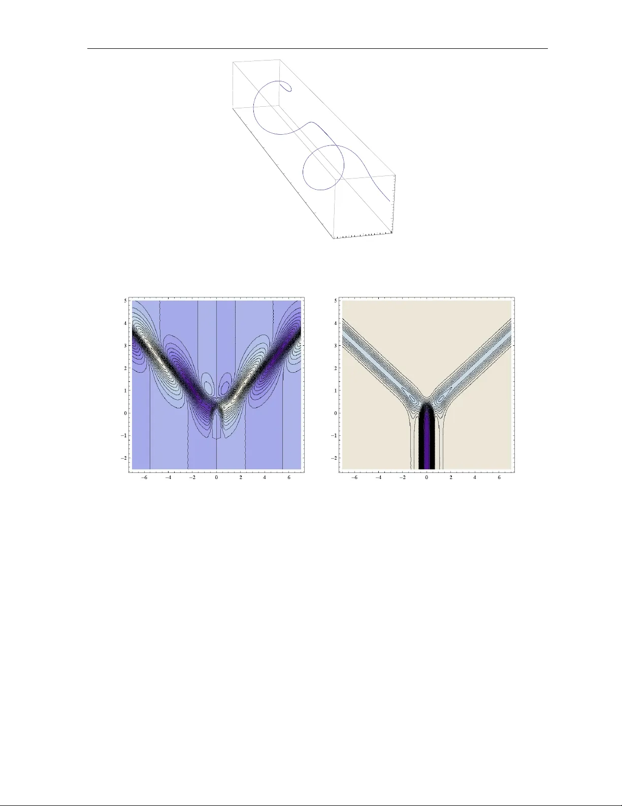
Symmetry , Integrabilit y and Geometry: Metho ds and Applications SIGMA 7 (2011), 096, 48 pages P olynomial Bundles and Generalised F ourier T ransforms for In tegrable Equations on A.I I I-t yp e Symmetric Spaces ? Vladimir S. GERDJIK O V † , Ge or gi G. GRAHOVSKI † , ‡ , Alexander V. MIKHAILO V § and Tihomir I. V ALCHEV † † Institute for Nucle ar R ese ar ch and Nucle ar Ener gy, Bulgarian A c ademy of Scienc es, 72 Tsarigr adsko chause e, Sofia 1784, Bulgaria E-mail: gerjikov@inrne.b as.b g , gr ah@inrne.b as.b g , valtchev@inrne.b as.b g ‡ Scho ol of Mathematic al Scienc es, Dublin Institute of T e chnolo gy, Kevin Str e et, Dublin 8, Ir eland § Applie d Math. Dep artment, University of L e e ds, Wo o dhouse L ane, L e e ds, LS2 9JT, UK E-mail: a.v.mikhailov@le e ds.ac.uk Receiv ed Ma y 26, 2011, in f inal form Octob er 04, 2011; Published online Octob er 20, 2011 h ttp://dx.doi.org/10.3842/SIGMA.2011.096 Abstract. A sp ecial class of integrable nonlinear dif feren tial equations related to A.I II -type symmetric spaces and having additional reductions are analyzed via the in v erse scattering metho d (ISM). Using the dressing method we construct t w o classes of soliton solutions asso ciated with the Lax op erator. Next, by using the W ronskian relations, the mapping b et w een the potential and the minimal sets of scattering data is constructed. F urthermore, completeness relations for the ‘squared solutions’ (generalized exp onentials) are deriv ed. Next, expansions of the p otential and its v ariation are obtained. This demonstrates that the interpretation of the inv erse scattering metho d as a generalized F ourier transform holds true. Finally , the Hamiltonian structures of these generalized multi-component Heisen b erg ferromagnetic (MHF) type integrable mo dels on A.I I I -t yp e symmetric spaces are brief ly analyzed. Key wor ds: reduction group; Riemann–Hilb ert problem; sp ectral decomp ositions; integrals of motion 2010 Mathematics Subje ct Classific ation: 37K20; 35Q51; 74J30; 78A60 Con ten ts 1 In tro duction 2 2 Preliminaries 4 2.1 Basic notations and general form of equations . . . . . . . . . . . . . . . . . . . . . . . . . 4 2.2 Direct scattering problem for the Lax op erator ( 2.3 ) . . . . . . . . . . . . . . . . . . . . . 6 3 Dressing metho d and soliton solutions 9 3.1 Rational dres sing . . . . . . . . . . . . . . . . . . . . . . . . . . . . . . . . . . . . . . . . . 9 3.2 One-soliton solutions . . . . . . . . . . . . . . . . . . . . . . . . . . . . . . . . . . . . . . . 13 3.3 Multisoliton solutions . . . . . . . . . . . . . . . . . . . . . . . . . . . . . . . . . . . . . . 16 ? This pap er is a con tribution to the Pro ceedings of the Conference “Symmetries and In tegrability of Dif ference Equations (SIDE-9)” (June 14–18, 2010, V arna, Bulgaria). The full collection is av ailable at h ttp://www.emis.de/journals/SIGMA/SIDE-9.h tml 2 V.S. Gerdjiko v, G.G. Graho vski, A.V. Mikhailo v and T.I. V alc hev 4 Generalized F ourier transform 18 4.1 Recursion operators and in tegrable hierarch y . . . . . . . . . . . . . . . . . . . . . . . . . 18 4.2 W ronskian relations and ‘squared solutions’ . . . . . . . . . . . . . . . . . . . . . . . . . . 21 4.3 The sk ew-scalar pro duct and the mapping M L 1 → T j . . . . . . . . . . . . . . . . . . . . 22 4.4 Recursion operators – an alternativ e approach . . . . . . . . . . . . . . . . . . . . . . . . . 24 5 Sp ectral theory of the recursion op erators 25 5.1 Asymptotics of the fundamental analytic solution . . . . . . . . . . . . . . . . . . . . . . . 25 5.2 Completeness of squared solutions . . . . . . . . . . . . . . . . . . . . . . . . . . . . . . . 26 5.3 Expansion ov er the ‘squared solutions’ . . . . . . . . . . . . . . . . . . . . . . . . . . . . . 29 5.4 Conjugation prop erties of the recursion op erator . . . . . . . . . . . . . . . . . . . . . . . 33 6 F undamen tal prop erties of the NLEE 34 6.1 In tegrals of motion . . . . . . . . . . . . . . . . . . . . . . . . . . . . . . . . . . . . . . . . 34 6.2 The hierarc hy of NLEE – Lax pair approac h . . . . . . . . . . . . . . . . . . . . . . . . . . 36 6.3 The hierarc hy of NLEE and generalized F ourier transforms . . . . . . . . . . . . . . . . . 38 6.4 Hierarc hy of Hamiltonian formulations . . . . . . . . . . . . . . . . . . . . . . . . . . . . . 40 7 Discussion and conclusions 42 A P arametrization of Gauss factors 43 References 46 1 In tro duction It is well kno wn [ 9 ], that t wo imp ortan t classes of integrable nonlinear evolution equations (NLEE) are related to symmetric spaces: the multi-component nonlinear Sc hr¨ odinger equations and their gauge equiv alent Heisenberg ferromagnet (HF) equations: iS t = 1 2 [ S, S xx ] , S 2 ( x, t ) = 1 1 . Here S takes v alues in some simple Lie algebra. In the simplest case of the algebra su (2) the function S describ es the spin of one-dimensional ferromagnet [ 4 ]. The HF’s equation is integrable in the sense of in v erse scattering transform [ 9 , 45 ]. Its Lax represen tation has the form: L ( λ ) ≡ i∂ x − λS , A ( λ ) ≡ i∂ t + iλ 2 [ S, S x ] + 2 λ 2 S. Since the time the complete integrabilit y of HF equations was discov ered, many attempts for constructing its generalization ha ve b een made [ 22 ]. The main goal of this pap er is to deriv e and analyze a sp ecial class of NLEE which is obtained from the HF type equations b y applying additional algebraic symmetries. A well kno wn metho d for constructing new integrable NLEE is based on the so-called re- duction group, in tro duced in [ 32 , 33 , 34 , 35 ] and further developed in [ 13 , 30 , 28 , 29 ]. It led to the discov ery of the 2-dimensional T oda f ield theories [ 34 , 36 ]. Its latest dev elopments of the metho d led to the disco v ery of new automorphic Lie algebras and their classif ication [ 30 , 28 , 29 ]. The hierarchies of integrable NLEE are generated b y the so-called recursion (generating) op erator. Such operators ha ve been constructed and analyzed for a wide class of Lax operators L and app eared to generate not only the Lax representations, but also the hierarc hy of NLEE’s related to a given Lax operator L , their conserv ation laws and their hierarc hy of Hamiltonian structures, see [ 7 , 40 , 45 , 20 , 21 ] and the n umerous references therein. Such op erators can P olynomial Bundles and GFT for Integrable Equations on A.I I I -type Symmetric Spaces 3 b e viewed also as Lax L op erators, taken in the adjoin t represen tation of the underlying Lie algebra g . The (generating) recursion op erator app eared f irst in the AKNS-approach [ 1 ] as a tool to generate the class of all A -op erators as w ell as the NLEE related to the giv en Lax op erator L ( λ ). Next, I.M. Gel’fand and L.A. Dic key [ 10 ] disco vered that the class of these A -op erators is con tained in the diagonal of the resolven t of L . The k ernel of the resolven t of L can be explicitly constructed in terms of the so-called fundamental analytic solutions (F AS), see [ 11 , 17 , 12 ]. The construction of the recursion op erator for Lax op erators, whose explicit dep endence on the spectral parameter λ is comparatively simple (sa y , linear, or quadratic) w as done a long time ago [ 1 , 27 , 15 , 16 ]. F urthermore, the completeness prop ert y for the set of eigenfunctions of the recursion operator (the ‘squared solutions’ of L ) is of paramount imp ortance. The complete- ness of the ‘squared solutions’ pla ys a fundamen tal role in pro ving that the inv erse scattering metho d is, in fact, a nonlinear analogue of the F ourier transform, which allows one to linearize the NLEE. Using these relations one is able to derive all fundamental prop erties of the NLEE on a common basis. In the symmetry approach to in tegrable equations the so-called ‘formal recursion op erator’ pla ys a crucial role. It has the general property to map a symmetry in to a symmetry of the giv en in tegrable NLEE [ 41 ]. If the considered NLEE possesses an inf inite hierarc hy of symmetries [ 26 ], or conserv ation laws [ 43 ] of arbitrary (high) order, or can b e linearized by a dif ferential substi- tution [ 44 ], then it has a formal recursion op erator [ 39 , 38 , 42 ]. F or an extensiv e and up-to-date surv eys on symmetry approach to in tegrability w e refer to [ 2 , 37 ] and the references therein. W e just note that in the Symmetry approach the formal recursion op erator do es not dep end on the b oundary conditions, imp osed on the p otential of the asso ciated Lax op erator. An alterna- tiv e approac h for construction of recursion operator from a given Lax op erator is presen ted b y M. G ¨ urses, A. Karasu and V. Sok olov in [ 24 ]. This metho d is pure algebraic, it is not related y et with the sp ectral theory of the Lax op erator L and it is not sensitive to the choice of the class of admissible p otentials of L . The problem of deriving recursion op erators b ecomes more dif f icult when we imp ose ad- ditional reductions on L . If this additional reduction is compatible with L , b eing linear or quadratic in λ , the construction of the recursion op erators is not a dif f icult task (see [ 20 ]; an alternativ e construction of Λ is giv en in [ 24 , 23 ]). The ef fect of the Z n -reduction is as follo ws: i) the relev an t ‘squared solutions’ hav e analyticity prop erties in sectors of the complex λ -plane closing angles π /n ; ii) the grading of the Lie algebra g ≡ ⊕ n − 1 k =0 g ( k ) is more in volv ed and as a consequence the recursion op erator is factorized into a pro duct of n factors Λ = n − 1 Q k =0 Λ k , and eac h of the factors Λ k maps Λ k : g ( k − 1) → g ( k ) . The applications of the dif feren tial geometric and Lie algebraic methods to soliton t yp e equa- tions led to the discov ery of a close relationship b et ween the m ulti-comp onen t (matrix) in te- grable equations (of nonlinear Sc hr¨ odinger t yp e) and the symmetric and homogeneous spaces [ 9 ]. Later on, this approach w as extended to other t yp es of multi-component in tegrable mo dels, lik e the deriv ative NLS, Kortew eg–de V ries and mo dif ied Kortew eg–de V ries, N -w av e, Dav ey– Stew artson, Kadomtsev–P etviash vili equations [ 3 , 8 ]. The purp ose of the presen t pap er is to derive nonlinear ev olution equations to generalize Heisen b erg’s mo del and study some of the prop erties of their Lax operators. W e are going to fo cus our attention on equations whose Lax representation is related to su (3). This pap er is a natural contin uation of our previous pap ers [ 18 , 19 , 14 ]. In Section 2 b elow w e give some of the necessary preliminaries. W e also study the Z 2 -reductions of the generalized Heisen b erg ferromagnets ( Z 2 -HF) related to symmetric spaces and outline the sp ectral pro- p erties of the relev ant Lax op erator and the construction of its fundamen tal analytic solutions. Section 3 is dedicated to the soliton solutions of the ( Z 2 -HF) mo dels. In their deriv ation w e mak e 4 V.S. Gerdjiko v, G.G. Graho vski, A.V. Mikhailo v and T.I. V alchev use of the dressing metho d [ 40 , 49 , 50 , 51 ]. Due to the additional reductions the Lax operator L ma y p ossess tw o types of discrete eigen v alues: generic ones, coming in quadruplets ± λ k , ± λ ∗ k and purely imaginary ones coming as doublets ± iκ j . Therefore we will hav e t wo t yp es of soliton solutions which w e will call quadruplet and doublet solitons respectively . W e outline the purely algebraic construction for deriving the N -soliton solutions for b oth types of solitons and pro vide the explicit expressions for the one-soliton solutions. Section 4 is dev oted to the deriv ation of the recursion op erators Λ. Here we f irst deriv e Λ using the G¨ urses–Karasu– Sok olov (GKS) method [ 24 ]. Next w e analyze the W ronskian relations as a basic to ol in the in verse scattering metho d [ 5 , 6 ]. F rom them, there naturally arise the ‘squared solutions’, which pla y a fundamental role also in the analysis of the mapping betw een the set of admissible p oten tials and the minimal sets of scattering data. The ‘squared solutions’ can also b e viewed as eigenfunctions of the recursion op erators Λ ± , whic h can b e used as an alternative def inition of the recursion op erators. One can c hec k that b oth approac hes lead to equiv alent expressions for Λ ± . Section 5 is dedicated to the sp ectral prop erties of the recursion operators. There we start b y pro ving the completeness relation for the ‘squared solutions’. Next we use this relation to derive the expansions of ad − 1 L 1 L 1 ,x , ad − 1 L 1 L 2 ,x and ad − 1 L 1 δ L 1 o ver the ‘squared solutions’. In the last Section 6 these expansions are treated as generalized F ourier transforms, allo wing one to linearize the NLEE. W e also demonstrate that all fundamen tal prop erties of the class of NLEE can b e formulated through the recursion operators. These include not only the description of the class of NLEE related to L , but also their integrals of motion and hierarc hy of Hamiltonian structures. W e end by discussion and conclusions. In App endix A w e hav e collected some useful form ulae for the Gauss factors of the scattering matrix and explicitly derive the op erator ad − 1 L 1 . 2 Preliminaries 2.1 Basic notations and general form of equations The main ob ject in our pap er is the following 2-comp onent system of NLEEs: iu t + u xx + ( uu ∗ x + v v ∗ x ) u x + ( uu ∗ x + v v ∗ x ) x u = 0 , iv t + v xx + ( uu ∗ x + v v ∗ x ) v x + ( uu ∗ x + v v ∗ x ) x v = 0 , (2.1) where the functions u : R × R → C and v : R × R → C are assumed to b e inf initely smo oth and satisfy the following b oundary conditions lim x →±∞ u ( x, t ) = 0 , lim x →±∞ v ( x, t ) = e iφ ± , φ ± ∈ R . (2.2) Moreo ver, u and v are not functionally indep enden t, but ob ey the constrain t | u | 2 + | v | 2 = 1. The system ( 2.1 ) represents a reduction of generalized Heisen b erg ferromagnet equations related to the symmetric space S U (3) /S ( U (1) × U (2)), see [ 18 , 19 ]. It p ossesses a zero curv ature represen tation with Lax op erators in the form L ( λ ) ≡ i∂ x + λL 1 ( x, t ) , (2.3) A ( λ ) ≡ i∂ t + λA 1 ( x, t ) + λ 2 A 2 ( x, t ) , (2.4) where λ is a sp ectral parameter and the matrix co ef f icients (p otentials) read L 1 =   0 u v u ∗ 0 0 v ∗ 0 0   , A 2 = 2 3 1 1 − L 2 1 = −   1 / 3 0 0 0 | u | 2 − 2 / 3 u ∗ v 0 v ∗ u | v | 2 − 2 / 3   , (2.5) P olynomial Bundles and GFT for Integrable Equations on A.I I I -type Symmetric Spaces 5 A 1 =   0 a b a ∗ 0 0 b ∗ 0 0   , a = iu x + i ( uu ∗ x + v v ∗ x ) u, b = iv x + i ( uu ∗ x + v v ∗ x ) v . (2.6) The sp ecif ic structure of the matrices ab ov e is a result of the simultaneous action of t w o Z 2 reductions on generic Lax op erators L and A , namely L † ( λ ∗ ) = − ˘ L ( λ ) , A † ( λ ∗ ) = − ˘ A ( λ ) , (2.7) C L ( − λ ) C = L ( λ ) , C A ( − λ ) C = A ( λ ) , C = diag (1 , − 1 , − 1) , (2.8) where the op eration ˘ is def ined as follows ˘ L ( λ ) ψ ( x, t, λ ) ≡ i∂ x ψ ( x, t, λ ) − λψ ( x, t, λ ) L 1 ( x, t, λ ) . The latter reduction represen ts Cartan’s inv olutive automorphism [ 25 , 31 ] in volv ed in the def i- nition of the symmetric space S U (3) /S ( U (1) × U (2)), that is, it induces a Z 2 -grading in the Lie algebra sl (3 , C ) sl (3) = sl 0 (3) ⊕ sl 1 (3) , sl σ (3) = { X ∈ g | C X C = ( − 1) σ X } . It is evident that the grading condition [ sl σ (3) , sl ς (3)] ⊂ sl σ + ς (mo d 2) (3) (2.9) is fulf illed. This grading will b e used widely in our further considerations. Due to the existence of the grading ( 2.9 ), any function X ( x, t, λ ) with v alues in sl (3) can b e represented in the form: X ( x, t, λ ) = X 0 ( x, t, λ ) + X 1 ( x, t, λ ) , X 0 , 1 ( x, t, λ ) ∈ sl 0 , 1 (3) . (2.10) Eac h comp onent X 0 , 1 , in its turn, splits in to a term commuting with L 1 and its orthogonal complemen t, namely X 0 = X 0 , ⊥ + κ 0 L 2 , L 2 = − A 2 = L 2 1 − 2 3 1 1 , h X 0 , ⊥ , L 2 i = 0 , (2.11) X 1 = X 1 , ⊥ + κ 1 L 1 , h X 1 , ⊥ , L 1 i = 0 . (2.12) The brack ets ab ov e stand for Killing form, def ined as: h X , Y i = tr( X Y ) . It is evident that the functions κ 0 and κ 1 can b e express ed as follows κ 0 = h X 0 , L 2 i h L 2 , L 2 i , κ 1 = h X 1 , L 1 i h L 1 , L 1 i . One can easily chec k that the norms of L 1 and L 2 are h L 1 , L 1 i = 2 , h L 2 , L 2 i = 2 3 and hence κ 0 and κ 1 are given by κ 0 = 3 2 h X 0 , L 2 i , κ 1 = 1 2 h X 1 , L 1 i . 6 V.S. Gerdjiko v, G.G. Graho vski, A.V. Mikhailo v and T.I. V alchev As we shall con vince ourselv es in some cases it pro ves to b e more con venien t to deal with Lax op erators ˜ L ( λ ) = i∂ x + U 0 ( x, t ) + λJ, J = diag(1 , 0 , − 1) , (2.13) ˜ A ( λ ) = i∂ t + ˜ A 0 ( x, t ) + λ ˜ A 1 ( x, t ) − λ 2 I , I = diag(1 / 3 , − 2 / 3 , 1 / 3) (2.14) gauge equiv alent to ( 2.3 ), ( 2.4 ). The gauge transformation, which puts L 1 and A 2 in to their diagonal form, is given b y the unitary matrix g = √ 2 2   1 0 − 1 u ∗ √ 2 v u ∗ v ∗ − √ 2 u v ∗   . F urther on w e are also going to use the explicit form of U 0 giv en by next form ula U 0 = ig − 1 g x = i 2   uu ∗ x + v v ∗ x √ 2( uv x − v u x ) uu ∗ x + v v ∗ x − √ 2( u ∗ v ∗ x − v ∗ u ∗ x ) 2( u ∗ u x + v ∗ v x ) − √ 2( u ∗ v ∗ x − v ∗ u ∗ x ) uu ∗ x + v v ∗ x √ 2( uv x − v u x ) uu ∗ x + v v ∗ x   . (2.15) 2.2 Direct scattering problem for the Lax op erator ( 2.3 ) Here we shall pro vide a short summary of some basic results and notions concerning the sp ec- tral theory of the Lax op erator L , the direct scattering problem and in tro duce the so-called fundamen tal analytic solutions. The sp ectral prop erties of L dep end on the choice of the class of admissible p oten tials, i.e. the potentials are a sub ject to certain b oundary condition. In the case of b oundary conditions of type ( 2.2 ), the con tinuous sp ectrum of L coincides with the real axis in the complex λ -plane, see [ 19 ]. In order to form ulate the direct scattering problem for L , one needs to introduce fundamental sets of solutions 1 ψ to the auxiliary (sp ectral) linear system L ( λ ) ψ ( x, t, λ ) = i∂ x ψ ( x, t, λ ) + λL 1 ( x, t ) ψ ( x, t, λ ) = 0 . (2.16) Since L ( λ ) and A ( λ ) comm ute, fundamental solutions ψ also satisfy the equation A ( λ ) ψ ( x, t, λ ) = i∂ t ψ ( x, t, λ ) + ( λA 1 ( x, t ) + λ 2 A 2 ( x, t )) ψ ( x, t, λ ) = ψ ( x, t, λ ) f ( λ ) . (2.17) The matrix-v alued function f ( λ ) = lim x →±∞ g − 1 ± ( λA 1 ( x, t ) + λ 2 A 2 ( x, t )) g ± = − λ 2 I (2.18) is called disp ersion law of the nonlinear equation. A sp ecial t yp e of fundamental solutions are the so-called Jost solutions ψ ± whic h are nor- malized as follows lim x →±∞ ψ ± ( x, t, λ ) e − iλJ x g − 1 ± = 1 1 , where g ± = lim x →±∞ g ( x, t ) = 1 √ 2   1 0 − 1 0 √ 2 e iφ ± 0 e − iφ ± 0 e − iφ ±   1 F urther w e shall simply call them fundamen tal solutions for short. P olynomial Bundles and GFT for Integrable Equations on A.I I I -type Symmetric Spaces 7 diagonalizes the asymptotics L 1 , ± = lim x →±∞ L 1 ( x, t ). Due to ( 2.18 ) one can sho w that the asymp- totic b eha vior of ψ ± do not dep end on t , i.e. the def inition is correct. The transition matrix T ( t, λ ) = [ ψ + ( x, t, λ )] − 1 ψ − ( x, t, λ ) . (2.19) is called scattering matrix. It can b e easily deduced from relation ( 2.17 ) that the scattering matrix evolv es with time according to the linear dif feren tial equation i∂ t T + [ f ( λ ) , T ] = 0 , whic h is integrated straigh t aw a y to give T ( t, λ ) = e if ( λ ) t T (0 , λ ) e − if ( λ ) t . Since the time parameter t do es not pla y a signif icant role in our further considerations, w e shall omit it (it will b e f ixed). The action of Z 2 -reductions ( 2.7 ), ( 2.8 ) imp oses the follo wing restrictions  ψ † ± ( x, λ ∗ )  − 1 = ψ ± ( x, λ ) ,  T † ( λ ∗ )  − 1 = T ( λ ) , (2.20) C ψ ± ( x, − λ ) C = ψ ± ( x, λ ) , C T ( − λ ) C = T ( λ ) (2.21) on the Jost solutions and the scattering matrix. F rom now on we will assume that φ + = φ − = 0. Hence the asymptotic v alues of L 1 and g b ecome equal to each other: L 1 , ± = L 1 , as , g + = g − = g as . The complex λ -plane is separated by the contin uous sp ectrum of L (real axis) into tw o regions of analyticit y: the upp er half plane C + and the lo wer one C − . W e are going to sk etc h tw o wa ys of constructing fundamen tal solutions (F AS) χ + ( x, λ ) and χ − ( x, λ ) which are analytic functions in C + and C − resp ectiv ely , see [ 19 ] for more detailed explanations. The f irst wa y is based on in tro ducing some auxiliary functions η ± ( x, λ ) = g − 1 as ψ ± ( x, λ ) e − iλJ x , whic h satisfy the auxiliary system: i∂ x η ± + U ( x, λ ) η ± ( x, λ ) − λη ± ( x, λ ) J = 0 , U ( x, λ ) = λg − 1 as L 1 ( x ) g as with the b oundary conditions lim x →±∞ η ± ( x, λ ) = 1 1. Equiv alently , η ± ( x, λ ) can b e regarded as solutions to the following V olterra-type in tegral equations: η ± ( x, λ ) = 1 1 + i Z x ±∞ dy e iλJ ( x − y ) [ U ( y , λ ) − λJ ] η ± ( y , λ ) e − iλJ ( x − y ) . Then we def ine ξ + ( x, λ ) as a solution to the following set of integral equations: ξ + kl ( x, λ ) = δ kl + i Z x −∞ dy e iλ ( J kk − J ll )( x − y )  ( U ( y , λ ) − λJ ) ξ + ( y , λ )  kl , k ≤ l , ξ + kl ( x, λ ) = i Z x ∞ dy e iλ ( J kk ( λ ) − J ll )( x − y )  ( U ( y , λ ) − λJ ) ξ + ( y , λ )  kl , k > l , and ξ − ( x, λ ) b eing a solution to ξ − kl ( x, λ ) = δ kl + i Z x ∞ dy e iλ ( J kk − J ll )( x − y )  ( U ( y , λ ) − λJ ) ξ − ( y , λ )  kl , k ≤ l , 8 V.S. Gerdjiko v, G.G. Graho vski, A.V. Mikhailo v and T.I. V alchev ξ − kl ( x, λ ) = i Z x −∞ dy e iλ ( J kk − J ll )( x − y )  ( U ( y , λ ) − λJ ) ξ − ( y , λ )  kl , k > l . It is easy to c heck that ξ + and ξ − ha ve the analytic prop erties in C + and C − resp ectiv ely due to the appropriate choice of the lo wer integration limits. The initial fundamen tal analytic solutions χ ± ( x, λ ) are obtained from ξ ± ( x, λ ) by applying the transformation: χ ± ( x, λ ) = g as ξ ± ( x, λ ) e iλJ x . (2.22) Another w ay of ho w one can construct F AS is by m ultiplying the Jost solutions b y appropriately c hosen matrices. It turns out that these matrix factors are inv olv ed in the Gauss decomp osition T ( λ ) = T ∓ ( λ ) D ± ( λ )( S ± ( λ )) − 1 (2.23) of the scattering matrix T ( λ ). Here is a list of all Gauss factors in a parametrization we are going to use further in our exp osition: S ± ( λ ) = exp s ± ( λ ) , T ± ( λ ) = exp r ± ( λ ) , s + ( λ ) =   0 s + α 1 s + α 3 0 0 s + α 2 0 0 0   , r + ( λ ) =   0 r + α 1 r + α 3 0 0 r + α 2 0 0 0   , s − ( λ ) =   0 0 0 s − α 1 0 0 s − α 3 s − α 2 0   , r − ( λ ) =   0 0 0 r − α 1 0 r − α 3 r − α 2 0   , D + ( λ ) = diag( m + 1 , m + 2 /m + 1 , 1 /m + 2 ) , D − ( λ ) = diag(1 /m − 2 , m − 2 /m − 1 , m − 1 ) , (2.24) where m + k ( λ ) (resp. m − k ( λ )) are the principal minors of T ( λ ) of order k = 1 , 2. Then χ + and χ − are expressed as follows χ ± ( x, λ ) = ψ − ( x, λ ) S ± = ψ + ( x, λ ) T ∓ ( λ ) D ± ( λ ) . The relation ab ov e can b e rewritten in the follo wing manner, using ( 2.22 ): ξ + ( x, λ ) = ξ − ( x, λ ) G ( x, λ ) , G ( x, λ ) = e iλJ x ( S − ) − 1 S + ( λ ) e − iλJ x . (2.25) Th us F AS can be regarded as solutions to a local Riemann–Hilbert problem. The established in terrelation b etw een the in verse scattering metho d and lo cal Riemann–Hilb ert problem pro ves to b e useful in constructing solutions to NLEEs. It can b e shown that the reduction conditions ( 2.20 ), ( 2.21 ) and equation ( 2.23 ) lead to the follo wing demands on the Gauss factors ( S + ( λ ∗ )) † = ( S − ( λ )) − 1 , ˜ C S ± ( − λ ) ˜ C = S ∓ ( λ ) , ( T + ( λ ∗ )) † = ( T − ( λ )) − 1 , ˜ C T ± ( − λ ) ˜ C = T ∓ ( λ ) , ˜ C = g as C g − 1 as =   0 0 1 0 1 0 1 0 0   , ( D + ( λ ∗ )) † = ( D − ( λ )) − 1 , ˜ C D ± ( − λ ) ˜ C = D ± ( λ ) . According to ( 2.24 ) these relations can b e also written as: ( s + ( λ ∗ )) † = − s − ( λ ) , ( r + ( λ ∗ )) † = − r − ( λ ) , ˜ C s + ( − λ ) ˜ C = s − ( λ ) , ˜ C r + ( − λ ) ˜ C = r − ( λ ) . Finally , com bining all this information w e see that the F AS ob ey the symmetry conditions ( χ + ) † ( x, λ ∗ ) = [ χ − ( x, λ )] − 1 , C χ + ( x, − λ ) C = χ − ( x, λ ) . P olynomial Bundles and GFT for Integrable Equations on A.I I I -type Symmetric Spaces 9 Remark 1. The Riemann–Hilbert problem allo ws singular solutions as w ell. The simplest types of singularities are simple p oles and zero es of the F AS and generically correspond to discrete eigen v alues of the Lax op erator L . Due to the reduction symmetries the discrete eigenv alues m ust form orbits of the reduction group. Generic orbits contain quadruplets, so if µ is an eigen v alue, then − µ and ± µ ∗ , are eigen v alues to o. How ev er, w e can hav e degenerate orbits to o. If the eigenv alue lies on the imaginary axis we will ha ve doublets of eigen v alues. 3 Dressing metho d and soliton solutions In the presen t section we are going to deriv e and analyze the 1-soliton solution to the 2- comp onen t system ( 2.1 ). F or this to b e done, we are going to apply the dressing method prop osed in [ 49 ] and developed in [ 50 , 51 , 34 , 35 ]. In the previous section (see Remark 1 ) w e established that the op erator L ma y p ossess tw o types of discrete eigenv alues: one, coming in quadruplets as well as purely imaginary ones coming as doublets ± iκ j . Therefore we will ha v e t wo types of soliton solutions: generic (or quadruplet) ones and doublet ones (kinks). 3.1 Rational dressing The idea of the dressing metho d is the follo wing. Firstly , one starts from known solutions u 0 ( x, t ), v 0 ( x, t ) of ( 2.1 ) and a solution ψ 0 ( x, t, λ ) of the auxiliary linear problems L (0) ( λ ) ψ 0 = i∂ x ψ 0 + λL (0) 1 ψ 0 = 0 , A (0) ( λ ) ψ 0 = i∂ t ψ 0 +  λA (0) 1 + λ 2 A (0) 2  ψ 0 = 0 , (3.1) where L (0) 1 , A (0) 1 and A (0) 2 ha ve the same form as given in ( 2.5 ), ( 2.6 ) but u and v are replaced by u 0 and v 0 resp ectiv ely . Then one constructs another function ψ 1 ( x, t, λ ) = Φ( x, t, λ ) ψ 0 ( x, t, λ ) whic h is assumed to b e a fundamental solution to a similar system of equations L (1) ( λ ) ψ 1 = i∂ x ψ 1 + λL (1) 1 ψ 1 = 0 , A (1) ( λ ) ψ 1 = i∂ t ψ 1 +  λA (1) 1 + λ 2 A (1) 2  ψ 1 = 0 . (3.2) The matrices L (1) 1 , A (1) 1 and A (1) 2 ha ve the same structure as L (0) 1 , A (0) 1 and A (0) 2 but instead of u 0 ( x, t ) and v 0 ( x, t ) one plugs some new solutions u 1 ( x, t ) and v 1 ( x, t ) to ( 2.1 ) whic h are to b e found. The dressing factor Φ( x, t, λ ) is assumed to b e regular at | λ | → 0 , ∞ . Due to the reduction conditions ( 2.7 ), ( 2.8 ) the dressing factor has the symmetries: C Φ( x, t, − λ ) C = Φ( x, t, λ ) , (3.3) Φ( x, t, λ )Φ † ( x, t, λ ∗ ) = 1 1 . (3.4) F rom ( 3.1 ) and ( 3.2 ) it follo ws that Φ( x, t, λ ) is a solution to the follo wing equations: i∂ x Φ + λL (1) 1 Φ − λ Φ L (0) 1 = 0 , (3.5) i∂ t Φ +  λA (1) 1 + λ 2 A (1) 2  Φ − Φ  λA (0) 1 − λ 2 A (0) 2  = 0 . (3.6) Since Φ( x, t, λ ) is regular at | λ | → ∞ from ( 3.5 ) one can derive the follo wing relation b etw een L (1) 1 and L (0) 1 : L (1) 1 ( x, t ) = Φ( x, t, ∞ ) L (0) 1 ( x, t )Φ † ( x, t, ∞ ) . (3.7) 10 V.S. Gerdjiko v, G.G. Graho vski, A.V. Mikhailo v and T.I. V alchev This equation will pla y a fundamental role in our further considerations since it allows one to generate a new solution to ( 2.1 ) from a giv en one. If w e consider a λ -indep endent dressing factor then from ( 3.5 ) and ( 3.6 ) we can deduce that Φ do not dep end on x and t either. Th us we hav e a simple rotation, related to the U (2) symmetry of the model. In order to get something more non trivial w e shall assume that Φ( x, t, λ ) is a rational function of λ with a minimal num b er of simple p oles. F rom the reduction condition ( 3.3 ) it follo ws that if µ is a p ole of Φ then − µ is a p ole to o. It is natural to assume that these p oles do not o verlap with the contin uous sp ectrum of L , i.e. Im µ 6 = 0. On the other hand ( 3.4 ) leads to the conclusion that Φ − 1 has p oles at µ ∗ and − µ ∗ . W e f irst consider the generic case when µ 6 = − µ ∗ , so the p oles of Φ do not coincide with the p oles of Φ − 1 and choose the following anzatz for the dressing factor and its inv erse: Φ( x, t, λ ) = 1 1 + λM ( x, t ) λ − µ + λ C M ( x, t ) C λ + µ , (3.8) Φ − 1 ( x, t, λ ) = 1 1 + λM † ( x, t ) λ − µ ∗ + λ C M † ( x, t ) C λ + µ ∗ . F rom ( 3.8 ) it follows that the matrix M satisf ies the following equation:  1 1 + µ ∗ M ( x, t ) µ ∗ − µ + µ ∗ C M ( x, t ) C µ ∗ + µ  M † ( x, t ) = 0 . (3.9) If we assume that the residue M is an in v ertible matrix (rank M = 3), then it is prop ortional to 1 1 and the dressing is trivial. In order to obtain a non-trivial dressing M ough t to b e singular. F or our purp oses it suf f ices to consider the case rank M = 1. Then the residue can be represen ted as a pro duct M = | n ih m | of a vector | n i = ( n 1 , n 2 , n 3 ) T and a co-v ector h m | = ( m ∗ 1 , m ∗ 2 , m ∗ 3 ). Substitution of this representation in to ( 3.9 ) leads to a linear equation for the vector | n i : | m i + µ ∗ | n ih m | m i µ ∗ − µ + µ ∗ | Cn ih m | Cm i µ ∗ + µ = 0 . (3.10) In tro duce the functions f 0 ( x, t ) = 1 ω h m ( x , t ) | m ( x , t ) i , f 1 ( x, t ) = 1 κ h m ( x , t ) | C | m ( x , t ) i , µ = ω + iκ. Then, the solution of ( 3.10 ) reads: | n ( x, t ) i = 2( if 1 ( x, t ) | m ( x , t ) i − f 0 ( x, t ) | C | m ( x , t ) i ) µ ∗ ( f 2 0 + f 2 1 ) . (3.11) The vector | m i is an element of the pro jective space C P 2 . Indeed, it is easily seen from ab ov e that a rescaling | m i → f | m i with an y nonzero complex f does not af fect the matrix M . T aking in to account the anzatz ( 3.8 ) one can rewrite ( 3.7 ) as: L (1) 1 = ( 1 1 + M + C M C ) L (0) 1 ( 1 1 + M + C M C ) † . (3.12) Notice that the dressing preserv es the matrix structure of the Lax operator L , since the dressing factor 1 1 + M + C M C is a blo ck-diagonal matrix. F rom this equality and from ( 3.12 ) it follows that the p otentials u 1 , v 1 can b e expresse d by u 0 , v 0 in the following wa y:  u 1 v 1  = M  u 0 v 0  , M = G µ ∗ ( G ∗ ) 2  H − F F ∗ H ∗  , (3.13) P olynomial Bundles and GFT for Integrable Equations on A.I I I -type Symmetric Spaces 11 where G = ω h m | m i + iκ h m | C | m i , H = | µ | 2 | m 1 | 2 + ( µ ∗ ) 2 | m 2 | 2 + µ 2 | m 3 | 2 , F = 4 iω κm 3 m ∗ 2 . It is easy to verify that the matrix M is unitary for a generic choice of µ and the nonzero v ector | m i . Th us we expressed all quantities needed in terms of | m i . It remains to f ind | m i itself. F or that purp ose we rewrite equations ( 3.5 ), ( 3.6 ) in the form: Φ( x, t, λ )  i∂ x + λL (0) 1  Φ − 1 ( x, t, λ ) = λL (1) 1 , Φ( x, t, λ )  i∂ t + λA (0) 1 + λ 2 A (0) 2  Φ − 1 ( x, t, λ ) = λA (1) 1 + λ 2 A (1) 2 . (3.14) It is ob viously satisf ied at λ = 0. F rom ( 3.14 ), it follows that the residues at λ = ± µ ∗ , λ = ± µ should v anish. It is suf f icient to v anish the residue at λ = µ ∗ (v anishing of the other residues follo ws from the symmetry conditions ( 3.3 )). Computing the residue at λ = µ ∗ and taking into accoun t equation ( 3.9 ), w e get  1 1 + µ ∗ M µ ∗ − µ + µ ∗ C M C µ ∗ + µ   i∂ x + µ ∗ L (0) 1  | m i = 0 , (3.15)  1 1 + µ ∗ M µ ∗ − µ + µ ∗ C M C µ ∗ + µ   i∂ t + µ ∗ A (0) 1 + ( µ ∗ ) 2 A (0) 2  | m i = 0 , (3.16) i.e. | m ( x, t ) i is an eigenfunction of the dressed Lax op erator. A general solution of equa- tions ( 3.15 ), ( 3.16 ) is | m ( x, t ) i = f ( x, t ) ψ 0 ( x, t ; µ ∗ ) | m 0 i , where f ( x, t ) is an arbitrary non-v anishing complex function and | m 0 i ∈ C 3 is a non-zero, but otherwise arbitrary complex v ector. Without an y loss of generalit y we can set f ( x, t ) = 1 (see the discussion ab ov e ab out the pro jective nature of the vector | m i . Th us we prov ed the following prop osition: Prop osition 1. L et u 0 ( x, t ) , v 0 ( x, t ) form a solution of the system ( 2.1 ) and ψ 0 ( x, t, λ ) b e a simultane ous fundamental solution of ( 3.1 ) . L et also Re µ 6 = 0 , Im µ 6 = 0 and | m 0 i ∈ C 3 b e a c omplex ve ctor. Then u 1 ( x, t ) , v 1 ( x, t ) given by ( 3.13 ) for m k b eing c omp onents of the ve ctor | m i = ψ 0 ( x, t, µ ∗ ) | m 0 i satisfy ( 2.1 ) as wel l. The c orr esp onding solution ψ 1 ( x, t, λ ) of the asso ciate d line ar system ( 3.2 ) is given by ψ 1 = Φ( x, t, λ ) ψ 0 ( x, t, λ ) wher e Φ( x, t, λ ) is define d by ( 3.8 ) , ( 3.11 ) , ( 3.15 ) and ( 3.16 ) . The new solution u 1 ( x, t ), v 1 ( x, t ) of equations ( 2.1 ) and the fundamen tal solution ψ 1 ( x, t ; λ ) of the corresp onding linear system are parameterized b y a complex num b er µ and a complex v ector | m 0 i ∈ C 3 . Let us no w consider the sp ecial case when µ = iκ . Then the sequence of steps nece ssary to determine Φ slightly changes. Indeed, supp ose w e hav e a dressing factor in the form: Φ( x, t, λ ) = 1 1 + λ  P ( x, t ) λ − iκ + C P ( x, t ) C λ + iκ  . (3.17) Due to the reduction ( 3.4 ) its in verse has the same poles as Φ itself and therefore the equation ΦΦ − 1 = 1 1 already contains second order p oles. V anishing of the p oles of second and f irst order resp ectiv ely leads to the follo wing algebraic conditions: P C P † = 0 , 12 V.S. Gerdjiko v, G.G. Graho vski, A.V. Mikhailo v and T.I. V alchev  1 1 + P + C P C 2  C P † C + P  1 1 + C P † C + P † 2  = 0 . (3.18) P is a degenerate matrix which means that it can b e presented as P = | q ih p | . Then the former algebraic constraint transforms into a quadratic relation for the vector | p i h p | C | p i = 0 . (3.19) Equation ( 3.18 ) is reduced to a linear system for | q i  1 1 + C | q ih p | C 2  C | p i = iσ | q i , where σ is some auxiliary real function to b e found. The ab o ve linear system allows one to express | q i through | p i and σ | q i =  iσ − h p | p i 2 C  − 1 C | p i . (3.20) In order to f ind | p i and σ we consider again the partial dif feren tial equations ( 3.14 ). The require- men t that the p oles of second and f irst order in ( 3.14 ) v anish iden tically yields to dif ferential relations for | p i and σ : i∂ x h p | − iν h p | L (0) 1 = 0 , i∂ t h p | − h p |  iν A (0) 1 + ( iν ) 2 A (0) 2  = 0 , i∂ x σ = κ h p | L (0) 1 C | p i , i∂ t σ = κ h p |  A (0) 1 + 2 iν A (0) 2  C | p i . It is not hard to v erify that | p ( x, t ) i and σ ( x, t ) are expressed through the initial solution ψ 0 ( x, t, λ ) as follows: | p ( x, t ) i = ψ 0 ( x, t, − iκ ) | p 0 i , (3.21) σ ( x, t ) = − κ h p 0 | ψ − 1 0 ( x, t, iκ ) ˙ ψ 0 ( x, t, iκ ) C | p 0 i + σ 0 , (3.22) where | p 0 i and σ 0 are constants of integration and ˙ ψ 0 := ∂ λ ψ 0 . After substituting ( 3.21 ) into ( 3.19 ) and taking in to accoun t the f irst Z 2 reduction w e see that the comp onents of the p olarization vector | p 0 i are no longer indep endent but satisfy the constrain t: h p 0 | C | p 0 i = 0 ⇔ | p 0 , 1 | 2 = | p 0 , 2 | 2 + | p 0 , 3 | 2 . (3.23) Th us to calculate the soliton solution itself one just substitutes the result for | p i and h p | in to M and uses formula ( 3.12 ). Now we are able to formulate a result quite similar to Prop o- sition 1 : Prop osition 2. L et it b e given functions u 0 ( x, t ) , v 0 ( x, t ) to satisfy ( 2.1 ) and ψ 0 ( x, t, λ ) to b e a fundamental solution of ( 3.1 ) . L et also κ ∈ R \{ 0 } , σ 0 ∈ R and | p 0 i b e a non-vanishing c omplex ve ctor satisfying ( 3.23 ) . Then u 1 ( x, t ) , v 1 ( x, t ) given by  u 1 v 1  = | p 1 | 2 + iσ ( | p 1 | 2 − iσ ) 2  iσ + | p 2 | 2 − | p 3 | 2 2 p ∗ 2 p 3 2 p 2 p ∗ 3 iσ − | p 2 | 2 + | p 3 | 2   u 0 v 0  , wher e p k ar e the c omp onents of the ve ctor | p i = ψ 0 ( x, t, − iκ ) | p 0 i is a solution of the system ( 2.1 ) to o. The solution ψ 1 ( x, t, λ ) of the line ar system ( 3.2 ) is given by ψ 1 = Φ ψ 0 wher e Φ is define d by ( 3.17 ) , ( 3.20 ) , ( 3.21 ) and ( 3.22 ) . As it is seen the new solution is parametrized b y the p olarization vector | m 0 i , the real n umber σ 0 and the p ole iκ . One can apply the dressing pro cedure repeatedly to build a sequence of exact solutions to the system whic h is parametrized by a set of complex constan ts µ k and constan t vectors | m k i ∈ C P 2 (resp. a set of real constants κ j , σ 0 ,j and complex three-vectors | p k i in the case of purely imaginary p oles). P olynomial Bundles and GFT for Integrable Equations on A.I I I -type Symmetric Spaces 13 3.2 One-soliton solutions Let us apply the dressing pro cedure to a trivial solution u 0 = 0, v 0 = 1 of equation ( 2.1 ). In this case ψ 0 ( x, t, λ ) =      cos( λx ) exp  − iλ 2 t 3  0 i sin( λx ) exp  − iλ 2 t 3  0 exp  2 iλ 2 t 3  0 i sin( λx ) exp  − iλ 2 t 3  0 cos( λx ) exp  − iλ 2 t 3       . (3.24) W e are going to consider the generic case f irst, i.e. we ha v e 4 distinct p oles of Φ and Φ − 1 to form a ‘quadruplet’ { µ, − µ, µ ∗ , − µ ∗ } . It is conv enient to decomp ose a constan t complex v ector | m 0 i according to the eigen-spaces of the endomorphism ψ 0 ( 3.24 ): | m 0 i = α   1 0 1   + β   1 0 − 1   + γ   0 1 0   , (3.25) where α , β , γ are arbitrary complex constants. If the v ector | m 0 i is prop ortional to one of the eigenv ectors of the endomorphism ψ 0 , then the corresp onding matrix M do es not dep end on the v ariables x and t (due to the pro jective nature of the v ector | m i ) and the corresp onding solution ( 3.13 ) is a simple unitary rotation of the constant solution u 0 = 0, v 0 = 1. Elemen tary solitons corresp ond to v ectors | m 0 i , b elonging to an essentially tw o-dimensional in v ariant subspaces of the endomorphism ψ 0 . In other words, elementary soliton solutions corresp ond to the choices of vector | m 0 i with only one zero co ef f icien t in the expansion ( 3.25 ). Let us consider each of these three cases in more detail. Case (i): α 6 = 0 , β 6 = 0 , γ = 0 In this case, the solution do es not dep end on the v ariable t . It follows from ( 3.13 ) that the solution can b e written in the following form u 1 = 0 , (3.26) v 1 =  ω ( | α | 2 e 2 κx + | β | 2 e − 2 κx ) + κ ( α ∗ β − β ∗ α ) sin(2 ω x ) + iκ ( α ∗ β + β ∗ α ) cos(2 ω x ) ω ( | α | 2 e 2 κx + | β | 2 e − 2 κx ) − κ ( α ∗ β − β ∗ α ) sin(2 ω x ) − iκ ( α ∗ β + β ∗ α ) cos(2 ω x )  2 . The function v 1 can b e written in the form v 1 = exp(4 iθ ( x )) where θ ( x ) = Arctan  κ cos(2 ω x + φ α − φ β ) ω cosh(2 κx + ln | α/β | )  , φ α = arg α, φ β = arg β . It is easy to chec k that u = 0, v = exp( if ( x )) is an exact solution of ( 2.1 ) for any dif ferentiable function f ( x ). It resem bles the case of the three-wa ve equation [ 48 ] where one w av e of an arbitrary shap e is an exact solution of the system and the t wo other w av es are identically zero. A plot of the solution ( 3.26 ) is shown on Fig. 1 . The solution ( 3.26 ) has a simple sp ectral c haracterization and an explicitly giv en analytic fundamental solution of the corresp onding linear problem. Case (ii): α 6 = 0 , β = 0 , γ 6 = 0 In this case, from ( 3.13 ) it follows that the solution can b e written in the form u 1 = 4 iω κQ ∗ exp { iω x + it ( κ 2 − ω 2 ) + i ( φ α − φ γ ) } ( ω − iκ ) Q 2 , v 1 = 1 − 8 ω κ 2 ( ω − iκ ) Q 2 , (3.27) 14 V.S. Gerdjiko v, G.G. Graho vski, A.V. Mikhailo v and T.I. V alchev - 1.0 - 0.5 0.0 0.5 1.0 - 5 0 5 - 1.0 - 0.5 0.0 0.5 1.0 Figure 1. Real and imaginary parts of v 1 (cf. form ula ( 3.26 )) as a function of x . Here κ = 1, ω = 10 − 3 , α = 1, β = 1 + i , γ = 0. Figure 2. Contour plot of Re v 1 ( x, t ) (left panel) and Re u 1 ( x, t ) (righ t panel)for a generic soliton solution (see formula 3.27 ) as a function of x and t where α = β = γ = κ = ω = 1. where Q = 2 ω e κ ( x − 2 ω t )+ln | α/γ | + ( ω + iκ ) e − κ ( x − 2 ω t ) − ln | α/γ | . Case (iii): α = 0 , β 6 = 0 , γ 6 = 0 The solution no w can b e obtained from the solution in the case (ii), b y changing α → β and x → − x . In the cases (ii) the solution ( 3.27 ) is a soliton of width 1 /κ moving with velocity 2 ω . The corresp onding soliton in the case (iii) mov es with a velocity − 2 ω . In the generic case, when all three constan ts are non-zero, the solution ( 3.13 ) represents a nonlinear interaction of the ab ov e describ ed solitons. F or κ > 0 it is a decay of unstable time indep enden t soliton from the case (i) in to tw o solitons, corresp onding to the cases (ii) and (iii) (see Fig. 2 ). F or κ < 0, the solution is a fusion of tw o colliding solitons into a stationary one. Let us now consider the case of imaginary p oles, i.e. µ = iκ . There exist t wo essentially dif ferent cases. P olynomial Bundles and GFT for Integrable Equations on A.I I I -type Symmetric Spaces 15 Figure 3. Plots of the phase Ξ( x ) (left panel) and Im v ( x ) (righ t panel) for a stationary doublet soliton solution ( 3.28 ) as a function of x and the phase φ where κ = σ 0 = 1. 1. Supp ose p 0 , 2 = γ = 0. Then from ( 3.23 ) it follows that | p 0 , 1 | = | p 0 , 3 | . It suf f ices to pick up p 0 , 1 = 1 and for the third component w e ha ve p 0 , 3 = exp( iϕ ), ϕ ∈ R . In this case the 1-soliton solution is stationary: u ( x ) = 0 , v ( x ) =  cosh 2 κx + sinh 2 κx cos ϕ + i ( σ 0 − 2 κx sin ϕ ) cosh 2 κx + sinh 2 κx cos ϕ − i ( σ 0 − 2 κx sin ϕ )  2 . The function v can b e presen ted as v ( x ) = exp(4 i Ξ( x )) , Ξ( x ) = arctan  σ 0 − 2 κx sin ϕ cosh 2 κx + sinh 2 κx cos ϕ  . (3.28) A plot of the solution ( 3.28 ) is shown on Fig. 3 . In particular, when ϕ = 0; π , i.e. p 0 , 1 = ± p 0 , 3 w e hav e for the doublet solution: u ( x ) = 0 , v ( x ) =  e ± 2 κx + iσ 0 e ± 2 κx − iσ 0  2 . It is eviden t that the presence of the constan t σ 0 here is essen tial since otherwise the solution coincides with the v acuum. 2. Now let us assume p 0 , 2 6 = 0. F or simplicity w e f ix p 0 , 2 = 1. Then the norms of p 0 , 1 and p 0 , 3 are interrelated through | p 0 , 1 | 2 − | p 0 , 3 | 2 = 1 . This is why it pro ves to b e con venien t to parametrize them as follows: p 0 , 1 = cosh θ 0 e i ( ϕ 0 + ˜ ϕ ) , p 0 , 3 = | sinh θ 0 | e i ( ϕ 0 − ˜ ϕ ) , θ 0 , ϕ 0 , ˜ ϕ ∈ R . The 1-soliton solution reads: u ( x, t ) = 2∆ ∗ ∆ 2 e i ( κ 2 t + ϕ 0 ) [sinh( κx + θ 0 ) cos ˜ ϕ + i sinh( κx − θ 0 ) sin ˜ ϕ ] , v ( x, t ) = ∆ ∗ (∆ ∗ − 2) ∆ 2 = 1 + 2(2 iσ − 1) ∆ + 4 iσ ( iσ − 1) ∆ 2 , where ∆( x, t ) = cosh 2 ( κx + θ 0 ) cos 2 ˜ ϕ + cosh 2 ( κx − θ 0 ) sin 2 ˜ ϕ − i ( σ 0 − 2 κ 2 t + κx sinh 2 θ 0 sin 2 ˜ ϕ ) , σ ( x, t ) = σ 0 − 2 κ 2 t + κx sinh 2 θ 0 sin 2 ˜ ϕ. 16 V.S. Gerdjiko v, G.G. Graho vski, A.V. Mikhailo v and T.I. V alchev Figure 4. Contour plot of Re u ( x, t ) (left panel) and Re v ( x, t ) (right panel) for doublet soliton solution of the type ( 3.29 ) as a function of x and t . Here κ = σ 0 = 1, θ 0 = 0 and ˜ ϕ = 0. The ab ov e solution can b e signif icantly simplif ied if one assumes that p 0 , 3 /p 0 , 1 ∈ R . In these b oundary cases the doublet solution reads: u ( x, t ) = 2  cosh 2 ( κx + θ 0 ) + i ( σ 0 − 2 κ 2 t )   cosh 2 ( κx + θ 0 ) − i ( σ 0 − 2 κ 2 t )  2 e i ( κ 2 t + ϕ 0 ) sinh( κx + θ 0 ) , v ( x, t ) =  cosh 2 ( κx + θ 0 ) + i ( σ 0 − 2 κ 2 t )   cosh 2 ( κx + θ 0 ) + iσ 0 − 2 − 2 iκ 2 t   cosh 2 ( κx + θ 0 ) − i ( σ 0 − 2 κ 2 t )  2 (3.29) if p 0 , 3 /p 0 , 1 > 0 ( ˜ ϕ = 0) and u ( x, t ) = 2  cosh 2 ( κx − θ 0 ) + i ( σ 0 − 2 κ 2 t )   cosh 2 ( κx − θ 0 ) − i ( σ 0 − 2 κ 2 t )  2 e i ( κ 2 t + ϕ 0 + π / 2 ) sinh( κx − θ 0 ) , v ( x, t ) =  cosh 2 ( κx − θ 0 ) + i ( σ 0 − 2 κ 2 t )   cosh 2 ( κx − θ 0 ) + iσ 0 − 2 − 2 iκ 2 t   cosh 2 ( κx − θ 0 ) − i ( σ 0 − 2 κ 2 t )  2 , when p 0 , 3 /p 0 , 1 < 0 ( ˜ ϕ = π / 2). A plot of the solution ( 3.29 ) is depicted on Fig. 4 . 3.3 Multisoliton solutions As w e mentioned ab o ve, the dressing pro cedure can b e applied several times consequen tly . Thus after dressing the 1-soliton solution one derives a 2-soliton solution, after dressing the 2-soliton solution one obtains a 3-soliton solution and so on. Of course, in doing this one is allo wed to apply either of dressing factors ( 3.8 ) and ( 3.17 ). Therefore the m ultisoliton solution will b e a certain combination of quadruplet and doublet solitons. Another w ay of deriv ation the m ultisoliton solution consists in using a dressing factor with m ultiple p oles. F or example, if one wan ts to generate N quadruplet solitons one should use a dressing factor in the form: Φ( x, t, λ ) = 1 1 + N X k =1 λ  M k ( x, t ) λ − µ k + C M k ( x, t ) C λ + µ k  , whic h is eviden tly compatible with the reduction condition ( 3.3 ). Due to ( 3.4 ) its inv erse has P olynomial Bundles and GFT for Integrable Equations on A.I I I -type Symmetric Spaces 17 the form: Φ − 1 ( x, t, λ ) = 1 1 + N X k =1 λ M † k ( x, t ) λ − µ ∗ k + C M † k ( x, t ) C λ + µ ∗ k ! . In order to determine the residues of Φ one follo ws the same steps as in the case of a 2-poles dressing factor. Firstly , the identit y ΦΦ − 1 = 1 1 implies that the residues of Φ and Φ − 1 satisfy certain algebraic relations, namely: M k " 1 1 + N X l =1 µ k M † l µ k − µ ∗ l + C M † l C µ k + µ ∗ l !# = 0 , k = 1 , . . . , N , (3.30) to ensure v anishing of the residue of ΦΦ − 1 at λ = µ k . Of course due to the Z 2 reductions w e will hav e an additional set of algebraic relations whic h are obtained from ( 3.30 ) by hermitian conjugation. As discussed b efore in order to obtain a nontrivial dressing the residues must b e degenerate matrices. Th us one in tro duces the factorization M k = | n k ih m k | and then reduces ( 3.30 ) to a linear system for | n k i | m k i = N X l =1 B lk | n l i , B lk := µ ∗ k  h m l | m k i µ l − µ ∗ k − h m l | C | m k i µ l + µ ∗ k C  . By solving it one can express the v ectors | n l i , l = 1 , . . . , N through all | m k i and that wa y determine the whole dressing factor in terms of | m k i . This step con tains the main tec hnical dif f iculty in the whole scheme. The v ectors | m k i can b e found from the natural requirement of v anishing of the p oles in the dif ferential equations ( 3.14 ). The result reads | m k ( x, t ) i = ψ 0 ( x, t, µ ∗ k ) | m k, 0 i . Th us we ha ve prov ed that as in the 2-p oles case the dressing factor is determined if one kno ws the seed solution ψ 0 ( x, t, λ ). The quadruplet N -soliton solution itself can b e deriv ed through the following formula L (1) 1 = 1 1 + N X k =1 ( M k + C M k C ) ! L (0) 1 1 1 + N X k =1 ( M k + C M k C ) ! † . F rom all said ab o v e it follows that the algorithm for obtaining the N -soliton solution can b e presen ted symbolically as follo ws L (0) 1 → ( | m 1 i , . . . , | m N i ) → ( | n 1 i , . . . , | n N i ) → ( M 1 , . . . , M N ) → L (1) 1 . Similarly , one is able to generate a sequence of N doublet solitons by making use of the follo wing factor Φ( x, t, λ ) = 1 1 + N X l =1 λ  P l ( x, t ) λ − iκ l + C P l ( x, t ) C λ + iκ l  . F ollowing the same steps as in the 1-soliton case one can con vince himself that the vectors | q l i in volv ed in the decomp osition P l = | q l ih p l | satisfy the linear system: C | p l i = N X s =1 D sl | q s i , 18 V.S. Gerdjiko v, G.G. Graho vski, A.V. Mikhailo v and T.I. V alchev where D ss := iσ s − h p s | p s i 2 C , D sl := κ l  h p s | C | p l i κ s − κ l − h p s | p l i κ s + κ l C  , s 6 = l. On the other hand the v ectors | p l i and the real functions σ l are expressed in terms of the initial solution ψ 0 and its deriv atives with resp ect to λ as follo ws: | p l ( x, t ) i = ψ 0 ( x, t, − iκ l ) | p l, 0 i , σ l ( x, t ) = − κ l h p l, 0 | ψ − 1 0 ( x, t, iκ l ) ˙ ψ 0 ( x, t, iκ l ) C | p l, 0 i + σ l, 0 , where | p l, 0 i and σ l, 0 for l = 1 , . . . , N are constan ts of integration to parametrize the solution. The comp onen ts of | p l i are not indep endent but satisfy h p l | C | p l i = 0 ⇒ h p l, 0 | C | p l, 0 i = 0 . In order to derive doublet N -soliton solution one uses: L (1) 1 = 1 1 + N X l =1 ( P l + C P l C ) ! L (0) 1 1 1 + N X l =1 ( P l + C P l C ) ! † . In this case the diagram which describ es the algorithm to obtain the m ultisoliton solution reads L (0) 1 → {| p l i , σ l } N l =1 → {| q l i} N l =1 → { P l } N l =1 → L (1) 1 . It is clear that apart of the ‘pure’ m ultisolitons discussed ab ov e there is a ‘mixed’ type of m ultisolitons, i.e. m ultisolitons to contain b oth sp ecies of 1-soliton solutions. In order to obtain suc h solution one needs to use a dressing factor p ossessing b oth types of p oles. 4 Generalized F ourier transform In this sec tion w e aim to dev elop the generalized F ourier transform in terpretation of the in verse scattering metho d for the Lax operator ( 2.3 ). F or this to b e done we are going to use some ba- sic notions lik e W ronskian relations, ‘squared solutions’, recursion op erators etc. The ‘squared solutions’ also kno wn as adjoin t solutions are generalizations of exponential functions in usual F ourier analysis, namely they are a complete system. They occur naturally in W ronskian rela- tions which interrelate the scattering data and the p otential L 1 ( x ) (as well as their v ariations) in a form which resembles a scalar pro duct and is called sk ew-scalar pro duct. The W ronskian relations allows one to express the expansion co ef f icients of L 1 ( x ) and its v ariation along these generalized exp onents in terms of the scattering data and its v ariations as we shall see later on. Within this framework the role of the operator id/dx whose eigenfunctions are exp( ik x ) is pla yed b y the recursion operators. W e shall presen t tw o substan tially dif feren t wa ys of obtaining the recursion op erators and compare them. 4.1 Recursion op erators and in tegrable hierarch y Recursion op erators app ear in man y situations in the theory of integrable systems [ 1 , 20 , 41 ]. Their existence is tigh tly related to the fact that eac h in tegrable NLEE b elongs to a whole family of inf inite num b er of in tegrable NLEEs asso ciated to the same Lax operator L . One can also assign to this family a whole inf inite set of symmetries and integrals of motion (Hamiltonians). In this subsection we are to derive the recursion op erators b y analyzing the interrelations b etw een mem b ers of the hierarch y of NLEEs. In doing this we are follo wing the ideas in [ 24 , 46 ]. P olynomial Bundles and GFT for Integrable Equations on A.I I I -type Symmetric Spaces 19 The hierarch y of in tegrable NLEEs asso ciated to L is generated through the zero curv ature represen tation which we rewrite in the original Lax form iL t = [ L, V ] . Eac h choice of V corresponds to an individual mem b er of the hierarch y . F ollowing the ideas in [ 24 ] we interrelate t wo adjacent f lows V and ˜ V through the equalit y ˜ V ( λ ) = k ( λ ) V ( λ ) + B ( λ ) , (4.1) where k ( λ ) is a scalar function and the remainder B has the structure of the Lax op erator A ( λ ) B ( λ ) = λB 1 + λ 2 B 2 . All quantities ab ov e m ust b e inv ariant with resp ect to the action of reductions ( 2.7 ), ( 2.8 ). This is why we pick up k ( λ ) = λ 2 while the op erator B ob ey the condition B † ( λ ∗ ) = B ( λ ) , C B ( − λ ) C = B ( λ ) . This means that the co ef f icients of B are hermitian matrices to fulf ill B 1 ∈ sl 1 (3), B 2 ∈ sl 0 (3). After substituting ( 4.1 ) into the Lax representation one obtains the following relation iL τ = iλ 2 L t + [ L, B ] , (4.2) where τ is the ev olution parameter of the f low ˜ V . Then the recursion op erator R is def ined as the mapping L 1 ,τ = R L 1 ,t . In order to f ind it w e need to solv e ( 4.2 ) and th us calculate the remainder B . Since relation ( 4.2 ) holds identically with resp ect to λ it splits in to the follo wing set of recurrence relations: iL 1 ,t + [ L 1 , B 2 ] = 0 , (4.3) iB 2 ,x + [ L 1 , B 1 ] = 0 , (4.4) L 1 ,τ − B 1 ,x = 0 . (4.5) In accordance with our conv en tions explained in the Preliminaries (see formulae ( 2.10 )–( 2.12 )) the co ef f icients B 1 and B 2 ha ve splittings B 1 = B ⊥ 1 + b 1 L 1 , h B ⊥ 1 , L 1 i = 0 , B 2 = B ⊥ 2 + b 2 L 2 , h B ⊥ 2 , L 2 i = 0 , (4.6) of terms B ⊥ 1 and B ⊥ 2 not commuting with L 1 and their orthogonal complements. After substi- tuting ( 4.6 ) into ( 4.3 ) it b ecomes p ossible to express B ⊥ 2 through L 1 ,t as follows: B ⊥ 2 = − i ad − 1 L 1 L 1 ,t , (4.7) where ad − 1 L 1 acts on the orthogonal parts only , i.e. the k ernel of ad L 1 is factorized. In this case it can b e prov en the presentation b elow holds true ad − 1 L 1 = 1 4  5 ad L 1 − ad 3 L 1  . 20 V.S. Gerdjiko v, G.G. Graho vski, A.V. Mikhailo v and T.I. V alchev The co ef f icient b 2 is determined from relation ( 4.4 ). Indeed, after plugging ( 4.6 ) into ( 4.4 ) w e get i∂ x B ⊥ 2 + ib 2 ,x L 2 + ib 2 L 2 ,x + [ L 1 , B 1 ] = 0 . (4.8) The L 1 -comm uting part of ( 4.8 ) is separated b y taking h · , L 2 i in both hand sides of the equation to give 2 3 b 2 ,x + h ∂ x B ⊥ 2 , L 2 i = 0 ⇒ b 2 = − 3 2 ∂ − 1 x h ∂ x B ⊥ 2 , L 2 i , (4.9) where w e hav e denoted by ∂ − 1 x the in tegral R x ±∞ dy . On the other hand by pro jecting ( 4.4 ) with π = ad − 1 L 1 ad L 1 one extracts its orthogonal part iπ ∂ x B ⊥ 2 + ib 2 L 2 ,x + [ L 1 , B ⊥ 1 ] = 0 . T aking in to account ( 4.9 ) one can f ind out the following recurrence relation B ⊥ 1 = Λ 2 B ⊥ 2 , Λ 2 = − i ad − 1 L 1  π ∂ x ( · ) − 3 2 L 2 ,x ∂ − 1 x h ∂ x ( · ) , L 2 i  . (4.10) F ormally speaking, one should write Λ ± 2 instead of Λ 2 for the in tegro-dif ferential op erator in- tro duced ab ov e since the lo wer integration limit in ∂ − 1 x dif fers. This choice of signs, ho wev er, is unessen tial for the considerations in the curren t subsection and this is wh y prefer a more simplif ied notation. After a similar treatment of ( 4.5 ) we obtain 2 b 1 ,x + h ∂ x B ⊥ 1 , L 1 i = 0 ⇒ b 1 = − 1 2 ∂ − 1 x h ∂ x B ⊥ 1 , L 1 i , L 1 ,τ = i ad L 1 Λ 1 B ⊥ 1 , Λ 1 = − i ad − 1 L 1  π ∂ x ( · ) − L 1 ,x 1 2 ∂ − 1 x h ∂ x ( · ) , L 1 i  . (4.11) Finally combining ( 4.7 ), ( 4.10 ) and ( 4.11 ) one derives L 1 ,τ = ad L 1 Λ 1 Λ 2 ad − 1 L 1 L 1 ,t ⇒ R = ad L 1 Λ 1 Λ 2 ad − 1 L 1 . (4.12) The recursion op erator can b e also presen ted conv eniently as a 4 × 4 matrix to map the column v ector ( u, v , u ∗ , v ∗ ) T t to the column v ector ( u, v , u ∗ , v ∗ ) T τ . Then it can be v erif ied that R ob eys the splitting: R = π A ( B loc + B nonl ) + K . The factors π and A lo ok as follows π =     1 − | u | 2 / 2 − uv ∗ / 2 − u 2 / 2 − uv / 2 − u ∗ v / 2 1 − | v | 2 / 2 − uv / 2 − v 2 / 2 − ( u ∗ ) 2 / 2 − u ∗ v ∗ / 2 1 − | u | 2 / 2 − u ∗ v / 2 − u ∗ v ∗ / 2 − ( v ∗ ) 2 / 2 − uv ∗ / 2 1 − | v | 2 / 2     , A := i∂ x     0 − v − u 0 − u 0 v 0 v ∗ 0 u ∗ 0 0 u ∗ − v ∗ 0     ∂ x . P olynomial Bundles and GFT for Integrable Equations on A.I I I -type Symmetric Spaces 21 The matrices B loc = i 4     0 − 4 u ∗ 2 v (3 | v | 2 − 1) − 6 u ∗ v 2 2 v ∗ (1 − 3 | v | 2 ) 6 u ( v ∗ ) 2 0 4 u − 4 u ∗ 0 3 u ( | v | 2 − | u | 2 ) − v (1 + 6 | u | 2 ) − u ∗ − v ∗ 0 0     and B nonl = − 3 i 4     2 u ∗ v 2 uv ∗ | u | 2 − | v | 2 − 1 / 3     ∂ − 1 x [( u ∗ x , v ∗ x , − u x , − v x )] are a lo cal and a nonlo cal part resp ectively originating from the orthogonal part B ⊥ 2 and the L 1 -comm uting part b 2 L 2 . Finally K = − 1 2     u v u ∗ v ∗     x ∂ − 1 x [( u ∗ , v ∗ , u, v ) A ( B loc + B nonl )] is connected with the term b 1 L 1 in the splitting of B 1 . 4.2 W ronskian relations and ‘squared solutions’ W ronskian relations [ 5 , 6 ] provide an important to ol for analyzing the relev ant class of NLEE and the mapping F : M → T , where M is the set of allo wed p otentials of L (in our case L 1 ) and T is the minimal set of scattering data. In deriving them w e will need along with the f irst equation in ( 2.16 ) also tw o other related equations: i ∂ ˆ χ ∂ x − λ ˆ χ ( x, λ ) L 1 ( x ) = 0 , ˆ χ ( x, λ ) ≡ χ − 1 ( x, λ ) , i ∂ δ χ ∂ x + λL 1 ( x ) δ χ ( x, λ ) + λδ L 1 ( x ) χ ( x, λ ) = 0 , where the v ariation of χ ( x, λ ) is due to the v ariation δ L 1 ( x ). The f irst type of W ronskian relations interrelates the asymptotics of F AS with L 1 and its p o w ers as shown in the examples b elow i ( ˆ χJ χ ( x, λ ) − J )   ∞ −∞ = λ Z ∞ −∞ dx ˆ χ [ L 1 , J ] χ ( x, λ ) , (4.13) ˆ χL 1 ( x ) χ ( x, λ )   ∞ −∞ = Z ∞ −∞ dx ˆ χL 1 ,x χ ( x, λ ) , (4.14) ˆ χL 2 ( x ) χ ( x, λ )   ∞ −∞ = Z ∞ −∞ dx ˆ χL 2 ,x χ ( x, λ ) . (4.15) W e remind the reader that J = diag(1 , 0 , − 1) and I = diag(1 / 3 , − 2 / 3 , 1 / 3) are the diagonal forms of (the asymptotics of ) L 1 and L 2 = L 2 1 − 2 1 1 / 3 resp ectively , that we in tro duced at the v ery b eginning in section Preliminaries (see formulae ( 2.13 ), ( 2.14 )). A second class of W ronskian relations connects the v ariation δ χ ( x, λ ) with the v ariation of L 1 , i.e. ˆ χδ χ ( x, λ )   ∞ −∞ = iλ Z ∞ −∞ dx ˆ χδ L 1 χ ( x, λ ) . 22 V.S. Gerdjiko v, G.G. Graho vski, A.V. Mikhailo v and T.I. V alchev In the left hand sides of the W ronskian relations are inv olved the scattering data and its v ariation while the right hand sides can b e view ed as F ourier type integrals. T o mak e this obvious let us tak e the Killing form of the W ronskian relation ( 4.13 ) with a Cartan–W eyl generator E α and use the inv ariance of the Killing form i h ˆ χJ χ ( x, λ ) − J, E α i   ∞ −∞ = λ Z ∞ −∞ dx h [ L 1 , J ] , e α ( x, λ ) i . The quantities e α ( x, λ ) = χE α ˆ χ ( x, λ ) in tro duced ab ov e are called ‘squared solutions’. Due to the fact that we hav e tw o F AS χ + ( x, λ ) and χ − ( x, λ ) w e obtain t wo types of ’squared solutions’ e ± α ( x, λ ). Similarly , taking the Killing form in ( 4.14 ) and ( 4.15 ) we f ind h ˆ χL 1 χ ( x, λ ) , E α i   ∞ −∞ = Z ∞ −∞ dx h L 1 ,x , e α ( x, λ ) i , (4.16) h ˆ χL 2 χ ( x, λ ) , E α i   ∞ −∞ = Z ∞ −∞ dx h L 2 ,x , e α ( x, λ ) i , (4.17) h ˆ χδ χ ( x, λ ) , E α i   ∞ −∞ = iλ Z ∞ −∞ dx h δ L 1 , e α ( x, λ ) i . (4.18) W e are interested more sp ecif ically in v ariations that are due to the time ev olution of L 1 ( x ), i.e. δ L 1 ( x ) = L 1 ( x, t + δ t ) − L 1 ( x, t ) ' δ t ∂ L 1 ∂ t . Therefore up to f irst order terms of δ t w e obtain h ˆ χχ t ( x, λ ) , E α i   ∞ x = −∞ = iλ Z ∞ −∞ dx h L 1 ,t , e α ( x, λ ) i . No w we can explain why the W ronskian relations are imp ortant for analyzing the mapping F : M L 1 → T . Indeed, taking χ ( x, λ ) to b e a fundamental analytic solution of L we can express the left hand sides of ( 4.16 ) and ( 4.17 ) (resp. ( 4.18 )) through the Gauss factors S ± , T ∓ and D ± (resp. through the Gauss factors and their v ariations). The right hand side of ( 4.16 ) and ( 4.17 ) (resp. ( 4.18 )) can be in terpreted as a F ourier-like transformation of the potential L 1 ( x ) (resp. of the v ariation δ L 1 ( x )). As a natural generalization of the usual exp onents there app ear the ‘squared solutions’. The ‘squared solutions’ are analytic functions of λ . This fact underlies the pro of of their completeness in the space of allow ed p otentials, as w e shall see. 4.3 The sk ew-scalar pro duct and the mapping M L 1 → T j It is obvious, that only some of the matrix elements of the squared solutions e α ( x, λ ) contribute to the right-hand sides of the W ronskian relations. T o make this clearer w e will use the Z 2 - grading of the Lie algebra which hin ts that we should split the squared solutions as in ( 2.10 ), namely: e α ( x, λ ) = H α ( x, λ ) + K α ( x, λ ) , H α ( x, λ ) ∈ sl 0 (3) , K α ( x, λ ) ∈ sl 1 (3) . (4.19) In addition, according to ( 2.11 ), ( 2.12 ) each comp onen ts H α ( x, λ ) and K α ( x, λ ) can b e split into H α ( x, λ ) = H α ( x, λ ) + h α L 2 ( x ) , h α = 3 2 h L 2 ( x ) , H α ( x, λ ) i , P olynomial Bundles and GFT for Integrable Equations on A.I I I -type Symmetric Spaces 23 K α ( x, λ ) = K α ( x, λ ) + k α L 1 ( x ) , k α = 1 2 h L 1 ( x ) , K α ( x, λ ) i , (4.20) where H α ( x, λ ) and K α ( x, λ ) do not comm ute with L 1 ( x ). It is not dif f icult to realize that only H α ( x, λ ) and K α ( x, λ ) contribute to the righ t-hand sides of the W ronskian relations. In what follows we will make use also of the skew-scalar pro duct   X , Y   = Z ∞ −∞ dy h X ( y ) , [ L 1 ( y ) , Y ( y )] i , where X and Y are functions with v alues in sl (3) / ker ad L 1 and v anishing for x → ±∞ . W e will denote the linear space of suc h functions b y M L 1 . Note, that w e can express the righ t hand sides of the W ronskian relations using the sk ew-scalar pro duct: h ˆ χL 1 χ ( x, λ ) , E α i   ∞ x = −∞ =   e α ( x, λ ) , ad − 1 L 1 L 1 ,x   , h ˆ χL 2 χ ( x, λ ) , E α i   ∞ x = −∞ =   e α ( x, λ ) , ad − 1 L 1 L 2 ,x   , h ˆ χδ χ ( x, λ ) , E α i   ∞ x = −∞ = iλ   e α ( x, λ ) , ad − 1 L 1 δ L 1   , h ˆ χχ t ( x, λ ) , E α i   ∞ x = −∞ = iλ   e α ( x, λ ) , ad − 1 L 1 L 1 ,t   . W e should also p oint out that the sk ew-scalar pro duct is non-degenerate on M L 1 . W e f inish this subsection b y listing the ef fective results from the W ronskian relations. Below α ∈ ∆ + : ρ (1) , ± α ( λ ) ≡ h ˆ D ± ˆ T ∓ J T ∓ D ± , E ± α i = −   ad − 1 L 1 L 1 ,x , K ± ± α ( x, λ )   , ρ (2) , ± α ( λ ) ≡ h ˆ D ± ˆ T ∓ I T ∓ D ± , E ± α i = −   ad − 1 L 1 L 2 ,x , H ± ± α ( x, λ )   ; (4.21) τ (1) , ± α ( λ ) ≡ h ˆ S ± J S ± , E ∓ α i =   ad − 1 L 1 L 1 ,x , K ± ∓ α ( x, λ )   , τ (2) , ± α ( λ ) ≡ h ˆ S ± I S ± , E ∓ α i =   ad − 1 L 1 L 2 ,x , H ± ∓ α ( x, λ )   ; (4.22) δ 0 ρ ± α ( λ ) ≡ h ˆ D ± ˆ T ∓ δ T ∓ D ± , E ± α i = − iλ   ad − 1 L 1 δ L 1 , K ± ± α ( x, λ )   , δ 0 τ ± α ( λ ) ≡ h ˆ S ± δ S ± , E ∓ α i = iλ   ad − 1 L 1 δ L 1 , K ± ∓ α ( x, λ )   . (4.23) In deriving the ab ov e form ulae, b esides the splitting ( 4.19 ) we also used the fact that ad − 1 L 1 δ L 1 , ad − 1 L 1 L 1 ,x ∈ sl 0 (3) and ad − 1 L 1 L 2 ,x ∈ sl 1 (3). The quantities ρ ( k ) , ± α , τ ( k ) , ± α , k = 1 , 2, can b e view ed as ref lection coef f icients. These formulae pro vide the basis in the analysis of the mapping M L 1 → T k , k = 1 , 2. Indeed L 1 ,x ∈ M L 1 , while the sets of co ef f icien ts T 1 ≡ T (1) 1 ∪ T (2) 1 , T ( k ) 1 ≡  τ ( k ) , ± α ( λ ) , λ ∈ R , α > 0  , T 2 ≡ T (1) 2 ∪ T (2) 2 , T ( k ) 2 ≡  ρ ( k ) , ± α ( λ ) , λ ∈ R , α > 0  completed with additional sets characterizing the discrete sp ectrum of L are candidates for the minimal sets of scattering data of the Lax op erator. The ab ov e considerations show, that following [ 1 ] w e can treat the ‘squared solutions’ as generalized exp onen tials. Therefore the mapping M L ! can b e viewed as a generalized F ourier transform. Of course, the justif ications of the ab ov e statemen ts m ust b e based on a pro of of the com- pleteness relation for the ‘squared solutions’ which will b e presen ted in the next section. 24 V.S. Gerdjiko v, G.G. Graho vski, A.V. Mikhailo v and T.I. V alchev 4.4 Recursion op erators – an alternativ e approach Our goal in this subsection is to presen t an alternativ e def inition of the recursion operators. W e introduce them as op erators Λ ± whose eigenfunctions are the ‘squared solutions’. More precisely , w e shall see that the following equality holds: Λ ± K ± α ( x, λ ) = λ 2 K ± α ( x, λ ) . Our consideration starts from analysis of the equation i∂ x e α + λ [ L 1 ( x ) , e α ( x, λ )] = 0 satisf ied b y eac h of the ‘squared solutions’. W e ha ve omitted the sup erscript ± in the notation of the squared solutions since it do es not pla y a signif ican t role in most of our further considerations. W e shall use it again at the end of subsection when it will b ecome essen tial. Due to the grading condition ( 2.9 ) the comp onents H α and K α are in terrelated through the system i∂ x H α + λ [ L 1 ( x ) , K α ( x, λ )] = 0 , i∂ x K α + λ [ L 1 ( x ) , H α ( x, λ )] = 0 . (4.24) After we extract terms prop ortional to L 1 from the ab ov e equations w e obtain h L 2 , ∂ x H α i + ∂ x h α = 0 ⇒ h α = h α, 0 − 3 2 ∂ − 1 x h L 2 , ∂ x H α i , h L 1 , ∂ x K α i + ∂ x k α = 0 ⇒ k α = k α, 0 − 1 2 ∂ − 1 x h L 1 , ∂ x K α i , where h α, 0 and k α, 0 are some in tegration constants. On the other hand the orthogonal part of ( 4.24 ) reads: iπ ∂ x H α + ih α L 2 ,x = − λ [ L 1 ( x ) , K α ] , iπ ∂ x K α + i k α L 1 ,x = − λ [ L 1 ( x ) , H α ] . After substituting h α and k α in the equations ab ov e w e get Λ 1 K α = λH α − k α, 0 Λ 2 L 2 , (4.25) Λ 2 H α = λK α − h α, 0 Λ 1 L 1 , (4.26) where the operators Λ 2 and Λ 1 are given in ( 4.10 ) and ( 4.11 ) resp ectively . This is the righ t place to mention that remark ably the operators Λ 1 , 2 are inv ertible. Indeed, they admit the factorization Λ 1 X = − i ad − 1 L 1 J 1 ∂ x X , J 1 X = X − 1 2 L 1 ,x ∂ − 1 x h L 1 , X i , Λ 2 Y = − i ad − 1 L 1 J 2 ∂ x Y , J 2 Y = X − 3 2 L 2 ,x ∂ − 1 x h L 2 , X i . It is not hard to see that the op erators J 1 and J 2 can b e inv erted as follo ws J − 1 1 X = X + 1 2 L 1 ,x ∂ − 1 x h L 1 , X i , J − 1 2 Y = X + 3 2 L 2 ,x ∂ − 1 x h L 2 , X i . Therefore Λ 1 and Λ 2 are inv ertible as w ell, namely Λ − 1 1 X = i∂ − 1 x J − 1 1 ad L 1 X , Λ − 1 2 X = i∂ − 1 x J − 1 2 ad L 1 Y . Let us apply Λ 2 to ( 4.25 ) and Λ 1 to ( 4.26 ). After restoring the index notation where needed the result reads: Λ ± 2 Λ ± 1 K ± α = λ 2 K ± α − λh α, 0 Λ ± 1 L 1 − k α, 0 Λ ± 2 Λ ± 2 L 2 , P olynomial Bundles and GFT for Integrable Equations on A.I I I -type Symmetric Spaces 25 Λ ± 1 Λ ± 2 H ± α = λ 2 H ± α − λk α, 0 Λ ± 2 L 2 − h α, 0 Λ ± 1 Λ ± 2 L 2 . This is the right place to remind the reader that the constants h α, 0 and k α, 0 are determined b y the asymptotic of the relev ant ‘squared solution’ for x → ∞ (or for x → −∞ ), dep ending on the prop er def inition of the recursion op erator. More detailed analysis shows that for eac h Λ ± 1 and Λ ± 2 there exist certain ro ots for which the constants k α, 0 and h α, 0 v anish. More sp ecif ically the following equalities holds: Λ + 1 K ± ∓ α ( x, λ ) = λH ± ∓ α ( x, λ ) , Λ − 1 K ± ± α ( x, λ ) = λH ± ± α ( x, λ ) , Λ + 2 H ± ∓ α ( x, λ ) = λK ± ∓ α ( x, λ ) , Λ − 2 K ± ± α ( x, λ ) = λK ± ± α ( x, λ ) for all ro ots α > 0 and therefore: Λ + 2 Λ + 1 K ± ∓ α ( x, λ ) = λ 2 K ± ∓ α ( x, λ ) , Λ − 2 Λ − 1 K ± ± α ( x, λ ) = λ 2 K ± ± α ( x, λ ) , Λ + 1 Λ + 2 H ± ∓ α ( x, λ ) = λ 2 H ± ∓ α ( x, λ ) , Λ − 1 Λ − 2 H ± ± α ( x, λ ) = λ 2 H ± ± α ( x, λ ) . The op erator Λ ± in tro duced as Λ ± X = Λ ± 1 Λ ± 2 X , X ∈ sl 0 (3) , ˜ Λ Y = Λ ± 2 Λ ± 1 Y , Y ∈ sl 1 (3) (4.27) is the recursion op erator w e ha ve b een lo oking for. If w e compare ( 4.27 ) and ( 4.12 ) we can conclude that both approaches lead to compatible results whic h coincide up to some conjugation b y ad L 1 . 5 Sp ectral theory of the recursion op erators 5.1 Asymptotics of the fundamen tal analytic solution F or p erforming the con tour integration, in order to derive the completeness relations for the squared solutions, one needs the asymptotics of the squared solutions for | λ | → ∞ . The starting p oin t here is the asymptotic expansion of the F AS for λ → ∞ : χ as ( x, λ ) = 1 1 + ∞ X k =1 χ k ( x ) λ − k . In tro duce: ˜ χ as ( x, λ ) = g − 1 ( x ) χ as ( x, λ ) e iJ λx , whic h satisfy: i d ˜ χ as dx + ig − 1 g x ˜ χ as ( x, λ ) + λ [ J, ˜ χ as ( x, λ )] = 0 . (5.1) T ogether with prop erly chosen asymptotic conditions ˜ χ as ( x, λ ) the last equation will provide the asymptotics of the fundamental analytic solution. Therefore it will allo w an asymptotic expansion of the form: ˜ χ as ( x, λ ) = ∞ X s =0 λ − s ˜ χ k, as ( x ) . This will lead to a recurrent relations for the expansion co ef f icients ˜ χ k, as ( x ). Inserting this expansion into equation ( 5.1 ) for the f irst tw o co ef f icients of ˜ χ as ( x, λ ) we get: [ J, ˜ χ 0 , as ( x )] = 0 , (5.2) 26 V.S. Gerdjiko v, G.G. Graho vski, A.V. Mikhailo v and T.I. V alchev i d ˜ χ 0 , as dx − ig − 1 x g ˜ χ 0 , as ( x ) + [ J, ˜ χ 1 , as ( x )] = 0 , (5.3) i d ˜ χ 1 , as dx − ig − 1 x g ˜ χ 1 , as ( x ) + [ J, ˜ χ 2 , as ( x )] = 0 . F rom ( 5.2 ) it follo ws that ˜ χ 0 , as ( x ) m ust b e a diagonal matrix and using the diagonal part of ( 5.3 ) one can derive it in an explicit form: ˜ χ 0 , as ( x ) = diag  e ρ ( x ) , e − 2 ρ ( x ) , e ρ ( x )  , ρ ( x ) = 1 2 Z x ±∞ dy ( u ∗ u y + v ∗ v y ) , (5.4) and for the of f-diagonal part of ˜ χ f 1 , as ( x ) we hav e (see equation ( 2.15 )): ˜ χ f 1 , as ( x ) = i 2   0 √ 2( uv x − v u x ) e − ρ ( x ) ( u ∗ u x + v ∗ v x ) e ρ ( x ) / 2 √ 2( u ∗ v ∗ x − v ∗ u ∗ x ) e ρ ( x ) 0 − √ 2( u ∗ v ∗ x − v ∗ u ∗ x ) e 2 ρ ( x ) − ( u ∗ u x + v ∗ v x ) e ρ ( x ) / 2 √ 2( v u x − uv x ) e − 2 ρ ( x ) 0   . As a result the asymptotic b eha vior of χ ( x, λ ) for λ → ∞ is giv en by: χ ( x, λ ) ' λ →∞ g ( x )  ˜ χ 0 , as ( x ) + 1 λ ˜ χ 1 , as ( x ) + · · ·  e − iJ λx . (5.5) Note, that the fundamen tal analytic solution χ ± do es not allow a canonical normalization for | λ | → ∞ . This dif f icult y can b e o v ercome by applying a suitable gauge transformation. Using the asymptotic b ehavior ( 5.5 ) of the F AS, one can derive the asymptotics of the squared solutions e α ( x, λ ) = ( χ ( x, λ ) E α χ − 1 ( x, λ )) f . Skipping the details: e ± α ( x, λ ) ' λ →∞ e i ( J,α ) λx g ( x ) ˜ χ as ( x ) E α ˜ χ − 1 as ( x ) g − 1 ( x ) = e i ( J,α ) λx +3 ρ ( x )( I ,α ) g ( x )  E α + O  λ − 1  g − 1 ( x ) . 5.2 Completeness of squared solutions Belo w we will derive the completeness relation for the ‘squared solutions’ for a class of p oten- tials L 1 ( x ) of the Lax op erator L which for every f ixed v alue of t satisfy the follo wing conditions: C1) L 1 ( x ) − L 1 , ± is complex v alued function of Sch wartz type, i.e. it is inf initely smo oth function of x falling of f for | x | → ∞ faster than an y p ow er of x ; C2) L 1 ( x ) is such that the corresponding functions m ± 1 ( λ ) and m ± 2 ( λ ) ha ve at most f inite num- b er of simple zero es. F or simplicity we assume also that m + 1 ( λ ) and m + 2 ( λ ) (resp. m − 1 ( λ ) and m − 2 ( λ )) hav e no common zero es; C3) the corresponding functions m ± 1 ( λ ) and m ± 2 ( λ ) ha ve no zero es on the real axis of the complex λ -plane. Remark 2. It is well known that the zero es of the functions m ± 1 ( λ ) and m ± 2 ( λ ) determine the discrete sp ectrum of L . The pro of of this fact comes out of the scop e of the present pap er. F or other classes of Lax op erators it is well known, see e.g. [ 11 , 20 ]. Belo w for def initeness w e in tro duce notations for the discrete eigen v alues. As we already men tioned, due to the tw o Z 2 -reductions, they are of t wo t yp es. Let there b e N 1 discrete eigen v alues of generic t yp e which come in quadruplets (see Fig. 5 ). W e will denote b y λ + 1 , λ + 2 , . . . , λ + N 1 those of them that are in the f irst quadrant, i.e. 0 < arg λ + k < π / 2, 1 ≤ k ≤ N 1 . The eigen v alues λ + N 1 + k = − ( λ + k ) ∗ b elong also to C + but are in the second quadran t. Besides we hav e also λ − j = ( λ + j ) ∗ , j = 1 , . . . , 2 N 1 whic h lie in C − . The second t yp e of discrete eigen v alues are P olynomial Bundles and GFT for Integrable Equations on A.I I I -type Symmetric Spaces 27 I  - - γ + γ − γ + , ∞ γ − , ∞ λ ◦ ◦ ◦ ◦ × × 6 - Figure 5. The bold line def ines the con tinuous spectrum of L , the regular lines show the integration con tours γ ± ; by γ ± , ∞ w e denote the ‘inf inite’ semi-circles. By ◦ we denote the discrete eigen v alues relev ant for one generic soliton whic h come in quadruplets ± λ ± j ; the second type of solitons corresp ond to purely imaginary pairs of discrete eigenv alues ± iν a denoted by × . purely imaginary , i.e. λ + 2 N 1 + a = iν a , a = 1 , . . . , N 2 ; obviously λ − 2 N 1 + a = − iν a . Therefore the Lax op erator L will hav e 4 N 1 + 2 N 2 discrete eigenv alues. Consider the Green function: G ± ( x, y , λ ) = G ± 1 ( x, y , λ ) θ ( y − x ) − G ± 2 ( x, y , λ ) θ ( x − y ) , (5.6) G ± 1 ( x, y , λ ) = X α ∈ ∆ + e ± ± α ( x, λ ) ⊗ e ± ∓ α ( y , λ ) , (5.7) G ± 2 ( x, y , λ ) = X α ∈ ∆ − e − ± α ( x, λ ) ⊗ e − ∓ α ( y , λ ) + r X j =1 h ± j ( x, λ ) ⊗ h ± j ( y , λ ) , (5.8) h ± j ( x, λ ) = χ ± ( x, λ ) H j ˆ χ ± ( x, λ ) . (5.9) In order to derive the completeness relations for the squared solutions, one needs to apply a contour integration to the integral: J G ( x, y ) = 1 2 π i I γ + dλ G + ( x, y , λ ) − 1 2 π i I γ − dλ G − ( x, y , λ ) , where the integration contours γ ± = R ∪ γ ± , ∞ are shown on Fig. 5 . Let us recall that the Lax operator L has t wo types of discrete eigenv alues whose n umber is 4 N 1 + 2 N 2 ; the f irst type corresp ond to generic solitons and come in quadruplets ± λ ± j ; the second t yp e corresp ond to purely imaginary pairs of discrete eigen v alues ± iν a . Thus according to Cauch y’s residuum theorem J G ( x, y ) = 2 N 1 + N 2 X k =1 Res λ = λ + k G + ( x, y , λ ) + Res λ = λ − k G − ( x, y , λ ) ! , presuming that the radii of the ‘inf inite’ semicircles are large enough so that all discrete eigen- v alues are inside the con tours γ ± . Condition C3 ab ov e ensures that G ± ( x, y , λ ) has no p oles on the contin uous sp ectrum. 28 V.S. Gerdjiko v, G.G. Graho vski, A.V. Mikhailo v and T.I. V alchev Next we integrate along the contours: J G ( x, y ) = 1 2 π i Z ∞ −∞ dλ ( G + ( x, y , λ ) − G − ( x, y , λ )) + 1 2 π i I γ + , ∞ dλ G + as ( x, y , λ ) − 1 2 π i I γ − , ∞ dλ G − as ( x, y , λ ) . In order to calculate the integrals o ver γ ± , ∞ it is enough to use the asymptotic b ehavior of the Green function for λ → ∞ . F rom equations ( 5.4 ) and ( 5.5 ) w e hav e: G ± 1 , as ( x, t, λ ) ' λ →∞ X α ∈ ∆ + e i ( J,α ) λ ( x − y )+3( ρ ( x ) − ρ ( y ))( I ,α ) × ( g ( x ) ⊗ g ( y ))  E ± α ⊗ E ∓ α + O ( λ − 1 )  ( g − 1 ( x ) ⊗ g − 1 ( y )) and G ± 2 , as ( x, t, λ ) ' λ →∞ r X j =1 ( g ( x ) ⊗ g ( y ))  H j ⊗ H ∨ j + O ( λ − 1 )  ( g − 1 ( x ) ⊗ g − 1 ( y )) + X α ∈ ∆ 0 ∪ ∆ − 1 e i ( J,α ) λ ( x − y )+3( ρ ( x ) − ρ ( y ))( I ,α ) ( g ( x ) ⊗ g ( y ))  E ± α ⊗ E ∓ α + O ( λ − 1 )  ( ˆ g ( x ) ⊗ ˆ g ( y )) . As a result we get: 1 2 π i I γ + , ∞ dλ G + as ( x, y , λ ) − 1 2 π i I γ − , ∞ dλ G − as ( x, y , λ ) = δ ( x − y ) ( g ( x ) ⊗ g ( y )) X α ∈ ∆ + ( E α ⊗ E − α − E − α ⊗ E α ) ( ˆ g ( x ) ⊗ ˆ g ( y )) . The next step is to simplify the integral along the con tinuous sp ectrum; namely we will calculate the jump of the Green function with the result: G + ( x, y , λ ) − G − ( x, y , λ ) = G + 1 ( x, y , λ ) − G − 1 ( x, y , λ ) = X α ∈ ∆ +  e + α ( x, λ ) ⊗ e + − α ( x, λ ) − e − − α ( x, λ ) ⊗ e − α ( x, λ )  . The pro of of this fact goes as follo ws. F rom the expression for the Green function (equa- tions ( 5.6 )–( 5.9 )) and using the relation θ ( x − y ) + θ ( y − x ) = 1 w e easily get: G + ( x, y , λ ) − G − ( x, y , λ ) = G + 1 ( x, y , λ ) − G − 1 ( x, y , λ ) − θ ( x − y )( G + 1 ( x, y , λ ) + G + 2 ( x, y , λ ) − G − 1 ( x, y , λ ) − G − 2 ( x, y , λ )) , so it will b e enough to pro ve that the co ef f icien t in front of θ ( x − y ) v anishes. Indeed, we ha ve: G + 1 ( x, y , λ ) + G + 2 ( x, y , λ ) − G − 1 ( x, y , λ ) − G − 2 ( x, y , λ ) = ( χ + ( x, λ ) ⊗ χ + ( y , λ ))Π 2 ( ˆ χ + ( x, λ ) ⊗ ˆ χ + ( y , λ )) − ( χ − ( x, λ ) ⊗ χ − ( y , λ ))Π 2 ( ˆ χ − ( x, λ ) ⊗ ˆ χ − ( y , λ )) . Here Π 2 = X α ∈ ∆ + ( E α ⊗ E − α + E − α ⊗ E α ) + 2 X k =1 H k ⊗ H k h H k , H k i P olynomial Bundles and GFT for Integrable Equations on A.I I I -type Symmetric Spaces 29 and H 1 = J , H 2 = J 4 . Note that Π 2 is the second Casimir endomorphism for the algebra sl (3). It remains to use equation ( 2.25 ) and the basic prop ert y of Π 2 that states: ( G ( λ ) ⊗ G ( λ ))Π 2 ( ˆ G ( λ ) ⊗ ˆ G ( λ )) = Π 2 , for any element G ( λ ) of the corresp onding group S L (3). W e ev aluate the con tribution from the discrete sp ectrum assuming that the squared solu- tions e ± α ( x, λ ) hav e at most simple poles at the p oints of the discrete sp ectrum. Therefore in the vicinity of the eigen v alues λ ± k w e use the follo wing expansions of the ‘squared solutions’: e ± α ( x, λ ) = ( λ − λ ± k ) p α e ± α,k λ − λ ± k + ˙ e ± α,k ! , where p α are integers and p α = − p − α . Th us we obtain: Res λ = λ + k G + ( x, y , λ ) = X α ∈ ∆ +  e ± α,k ⊗ ˙ e ± − α,k + ˙ e ± α,k ⊗ e ± − α,k  . Therefore the completeness relations tak es the form: δ ( x − y ) ( g ( x ) ⊗ g ( y )) Π 0 ( ˆ g ( x ) ⊗ ˆ g ( y )) = i 2 π Z ∞ −∞ dλ X α ∈ ∆ +  e + α ( x, λ ) ⊗ e + − α ( x, λ ) − e − − α ( x, λ ) ⊗ e − α ( x, λ )  + 2 N 1 + N 2 X k =1 X α ∈ ∆ +  e + α,k ( x ) ⊗ ˙ e + − α,k ( y ) + ˙ e + α,k ( x ) ⊗ e + − α,k ( y ) + e − − α,k ( x ) ⊗ ˙ e − α,k ( y ) + ˙ e − − α,k ( x ) ⊗ e − α,k ( y )  , (5.10) where Π 0 = X α ∈ ∆ + E α ⊗ E − α − E − α ⊗ E α ( α, J ) and e ± α,k = e − α ( x, λ ± k ) , ˙ e ± α,k = ∂ e ± α ( x, λ ) ∂ λ     λ = λ ± k . 5.3 Expansion o ver the ‘squared solutions’ Using the completeness relations of the squared solutions, one can expand any generic ele- men t F ( x ) of the phase space M o ver the complete sets of squared solutions. W e remind that F ( x ) is a generic elemen t of M if it tends fast enough to zero for | x | → ∞ and is ‘p erp en- dicular’, i.e. h F ( x ) , L 1 i = h F ( x ) , L 2 i = 0 . It can b e parametrized as follo ws: F ( x ) = g ( x ) X α ∈ ∆ + ∪ ∆ − F α ( x ) E α g ( x ) . 30 V.S. Gerdjiko v, G.G. Graho vski, A.V. Mikhailo v and T.I. V alchev Let us no w m ultiply b oth sides of the completeness relation ( 5.10 ) by 1 1 ⊗ [ L 1 ( y ) , F ( y )] on the righ t, take the Killing form of the second factors in the tensor pro duct and integrate o ver y . In the left hand side after some manipulations we get: Z ∞ −∞ dy h ( g ( x ) ⊗ g ( y ))Π 0 ( ˆ g ( x ) ⊗ ˆ g ( y )) , 1 1 ⊗ [ L 1 ( y ) , F ( y )] i 2 δ ( x − y ) = g ( x ) X α ∈ ∆ + ∪ ∆ − E α ( α, J ) ˆ g ( x ) Z ∞ −∞ dy h g ( y ) E − α ˆ g ( y ) , [ L 1 ( y ) , F ( y )] i δ ( x − y ) = g ( x ) X α ∈ ∆ + ∪ ∆ − F α ( x ) E α ˆ g ( x ) = F ( x ) . The same op erations applied to the right hand sides of ( 5.10 ) replaces each of the terms e ± α ( x, λ ) ⊗ e ± − α ( y , λ ) by e ± α ( x, λ )   e ± α ( y , λ ) , F ( y )   . Th us the expansion co ef f icients of F ( x ) are provided by its skew-scalar pro ducts with the ‘squared solutions’. The result is: F ( x ) = i 2 π Z ∞ −∞ dλ X α ∈ ∆ +  e + α ( x, λ ) γ + F ; α ( λ ) − e − − α ( x, λ ) γ − F ; α ( λ )  + 2 N 1 + N 2 X k =1 X α ∈ ∆ + 1  Z + F ; α,k ( x ) + Z − F ; α,k ( x )  , (5.11) where γ ± F ; α ( λ ) =   e ± ∓ α ( y , λ ) , F ( y )   , Z ± F,α ; k ( x ) = e ± ± α ; k ( x ) ˙ γ ± F,α ; k + ˙ e ± ± α ; k ( x ) γ ± F,α ; k , γ ± F,α ; k =   e ± ∓ α ; k ( y ) , F ( y )   , ˙ γ ± F,α ; k =   ˙ e ± ∓ α ; k ( y ) , F ( y )   . (5.12) Similarly , exchanging x and y , m ultiplying b oth sides of the completeness relation ( 5.10 ) by [ L 1 ( y ) , F ( y )] ⊗ 1 1 on the right, take the Killing form of the f irst factors in the tensor pro duct and integrate ov er y w e get: F ( x ) = − i 2 π Z ∞ −∞ dλ X α ∈ ∆ +  e + α ( x, λ ) θ + F ; α ( λ ) − e − − α ( x, λ ) θ − F ; α ( λ )  − 2 N 1 + N 2 X k =1 X α ∈ ∆ + 1 ( Y + F ; α,k ( x ) + Y − F ; α,k ( x )) , (5.13) where θ ± F ; α ( λ ) =   e ± ± α ( y , λ ) , F ( y )   , Y ± F,α ; k ( x ) = e ± ∓ α ; k ( x ) ˙ θ ± F,α ; k + ˙ e ± ∓ α ; k ( x ) θ ± F,α ; k , θ ± F,α ; k =   e ± ± α ; k ( y ) , F ( y )   , ˙ θ ± F,α ; k =   ˙ e ± ± α ; k ( y ) , F ( y )   . (5.14) The completeness relation ( 5.11 ) allo ws one to pro ve the following Corollary 1. i ) The function F ( x ) ≡ 0 if and only if al l its exp ansion c o efficients ( 5.12 ) vanish, i.e.: γ + F ; − α ( λ ) = γ − F ; α ( λ ) = 0 , α ∈ ∆ + ; Z + F,α ; k ( x ) = Z − F,α ; k ( x ) = 0 , k = 1 , . . . , ˜ N , (5.15) wher e ˜ N = 2 N 1 + N 2 . P olynomial Bundles and GFT for Integrable Equations on A.I I I -type Symmetric Spaces 31 ii ) The function F ( x ) ≡ 0 if and only if al l its exp ansion c o efficients ( 5.14 ) vanish, i.e.: θ + F ; − α ( λ ) = θ − F ; α ( λ ) = 0 , α ∈ ∆ + ; Y + F,α ; k ( x ) = Y − F,α ; k ( x ) = 0 , k = 1 , . . . , ˜ N . Pro of . Inserting F ( x ) ≡ 0 into the r.h.s. of the inv ersion formulae ( 5.12 ) w e obtain the rela- tions ( 5.15 ). Next, let us assume that equation ( 5.15 ) holds and let us insert it into the r.h.s. of equation ( 5.11 ). This immediately giv es F ( x ) = 0. Thus i ) is pro ved. ii ) is pro ved analogously using equations ( 5.14 ) and ( 5.13 ).  In other words w e established an one-to-one corresp ondence b etw een the element F ( x ) ∈ M and its expansion co ef f icien ts. No w, let us take F ( x ) = ad − 1 L 1 L j,x ( x ), j = 1 , 2. Then the corresp onding expansion co ef f icien ts are given by: ρ ( j ) , ± α ( λ ) =   e ± ± α ( x, λ ) , ad − 1 L 1 L j,x   , ρ ( j ) , ± α ; k = 0 , ˙ ρ ( j ) , ± α ; k =   ˙ e ± ± α ; k ( x ) , ad − 1 L 1 L j,x   , τ ( j ) , ± α ( λ ) = −   e ± ∓ α ( x, λ ) , ad − 1 L 1 L j,x   , τ ( j ) , ± α ; k = 0 , ˙ τ ( j ) , ± α ; k = −   ˙ e ± ∓ α ; k ( x ) , ad − 1 L 1 L j,x   . F rom the W ronskian relations w e hav e : ρ (1) , ± α ( λ ) = h ˆ D ± ˆ T ∓ J T ∓ D ± , E ∓ α i , ρ (1) , ± α ; k = 0 , ˙ ρ (1) , ± α ; k = h ˆ D ± ˆ T ∓ J T ∓ D ± , E ∓ α i , ρ (2) , ± α ( λ ) = 3 h ˆ D ± ˆ T ∓ I T ∓ D ± , E ∓ α i , ρ (2) , ± α ; k = 0 , ˙ ρ (2) , ± α ; k = 3 h ˆ D ± ˆ T ∓ I T ∓ D ± , E ∓ α i . T aking into accoun t that ad − 1 L 1 L 1 ,x ( x ) ∈ sl (0) and ad − 1 L 1 L 2 ,x ( x ) ∈ sl (1) w e obtain the following expansions of these functions o ver the ‘squared solutions’ (for details see the app endix): ad − 1 L 1 L 1 ,x ( x ) = i 2 π Z ∞ −∞ dλ X α ∈ ∆ + ( α, J )  s + α ( λ ) H + α ( x, λ ) + s − α ( λ ) H − − α ( x, λ )  − N X k =1 X α ∈ ∆ + ( α, J )  s + α ; k H + α ; k ( x ) − s − α ; k H − − α ; k ( x )  , ad − 1 L 1 L 1 ,x ( x ) = − i 2 π Z ∞ −∞ dλ X α ∈ ∆ + ( α, J )  r + α ( λ ) H + − α ( x, λ ) + r − α ( λ ) H − α ( x, λ )  + N X k =1 X α ∈ ∆ + ( α, J )  r + α ; k H + − α ; k ( x ) − r − α ; k H − α ; k ( x )  . Similarly: ad − 1 L 1 L 2 ,x ( x ) = i 2 π Z ∞ −∞ dλ X α ∈ ∆ +  τ (2)+ α ( λ ) K + α ( x, λ ) − τ (2) , − α ( λ ) K − − α ( x, λ )  − N X k =1 X α ∈ ∆ +  τ (2) , + α ; k K + α ; k ( x ) + τ (2) , − α ; k K − − α ; k ( x )  , ad − 1 L 1 L 2 ,x ( x ) = − i 2 π Z ∞ −∞ dλ X α ∈ ∆ +  ρ (2)+ α ( λ ) K + − α ( x, λ ) − ρ (2) , − α ( λ ) K − α ( x, λ )  + N X k =1 X α ∈ ∆ +  ρ (2) , + α ; k K + − α ; k ( x ) + ρ (2) , − α ; k K − α ; k ( x )  . 32 V.S. Gerdjiko v, G.G. Graho vski, A.V. Mikhailo v and T.I. V alchev Here τ (2) , ± α ( λ ) = ± ( α, I ) s ± α ( λ ) for α ∈ δ + 1 , τ (2) , ± α 3 ( λ ) = s ± α 1 s ± α 2 ( λ ) , τ (2) , ± α ; k = Res λ = λ ± k τ (2) , ± α ( λ ) , ρ (2) , ± α ( λ ) = ± ( α, I ) r ± α ( λ ) for α ∈ δ + 1 , ρ (2) , ± α 3 ( λ ) = r ± α 1 r ± α 2 ( λ ) , ρ (2) , ± α ; k = Res λ = λ ± k ρ (2) , ± α ( λ ) and δ + 1 = { α 1 , α 2 } . Next, taking F ( x ) = ad − 1 L 1 δ L 1 ( x ) we derive the corresp onding expansions of the v ariation of L 1 ( x ) ov er the squared solutions. Thus we obtain the following expansions for ad − 1 L 1 δ L 1 ( x ): i ad − 1 L 1 δ L 1 ( x ) = − 1 2 π Z ∞ −∞ dλ λ X α ∈ ∆ +  H + α ( x, λ ) δ 0 τ (1)+ α ( λ ) − H − − α ( x, λ ) δ τ (1) − α ( λ )  − N X k =1 X α ∈ ∆ + ( 1 λ + k " H + α ; k ( x ) δ 0 τ + α ; k − τ + α ; k δ λ + k λ + k ! + ˙ H + α ; k ( x ) τ + α ; k δ λ + k # + 1 λ − k " H − − α ; k ( x ) δ 0 τ − α ; k − τ − α ; k δ λ − k λ − k ! + ˙ H − − α ; k ( x ) τ − α ; k δ λ − k #) , i ad − 1 L 1 δ L 1 ( x ) = 1 2 π Z ∞ −∞ dλ λ X α ∈ ∆ +  H + − α ( x, λ ) δ 0 ρ (1)+ α ( λ ) − H − α ( x, λ ) δ ρ (1) − α ( λ )  + N X k =1 X α ∈ ∆ + ( 1 λ + k " H + − α ; k ( x ) δ 0 ρ + α ; k − ρ + α ; k δ λ + k λ + k ! + ˙ H + − α ; k ( x ) ρ + α ; k δ λ + k # + 1 λ − k " H − α ; k ( x ) δ 0 ρ − α ; k − ρ − α ; k δ λ − k λ − k ! + ˙ H − α ; k ( x ) ρ − α ; k δ λ − k #) . The corresp onding expansion co ef f icients are giv en by: δ 0 τ ± α ( λ ) = δ s ± α ( λ ) for α ∈ δ + 1 , δ 0 τ ± α 3 ( λ ) = δ s ± α 3 ± 1 2 ( δ s ± α 1 s ± α 2 − s ± α 1 δ s ± α 2 ) , δ 0 ρ ± α ( λ ) = δ r ± α ( λ ) for α ∈ δ + 1 , δ 0 ρ ± α 3 ( λ ) = δ r ± α 3 ± 1 2 ( δ r ± α 1 r ± α 2 − s ± α 1 δ s ± α 2 ) . The calculation of the expansion co ef f icient for the discrete sp ectrum is explained in the ap- p endix. Presuming that the v ariation of the p otential is due to the time evolution of L 1 ( x ): δ L 1 ( x ) = L 1 ( x, t + δ t ) − L 1 ( x, t ) ' δ t ∂ L 1 ∂ t , one can get similar expansions for the time-deriv ativ e ad − 1 L 1 L 1 ,t ( x ): i ad − 1 L 1 L 1 ,t ( x ) = 1 2 π Z ∞ −∞ dλ λ X α ∈ ∆ +  δ t τ + α ( λ ) H − α ( x, λ ) − δ t τ − α ( λ ) H α ( x, λ )  − N X k =1 X α ∈ ∆ + ( 1 λ + k " H + α ; k ( x ) δ t τ + α ; k − τ + α ; k λ + k,t λ + k ! + ˙ H + α ; k ( x ) τ + α ; k λ + k,t # P olynomial Bundles and GFT for Integrable Equations on A.I I I -type Symmetric Spaces 33 + 1 λ − k " H − − α ; k ( x ) δ t τ − α ; k − τ − α ; k λ − k,t λ − k ! + ˙ H − − α ; k ( x ) τ − α ; k λ − k,t #) and i ad − 1 L 1 L 1 ,t ( x ) = 1 2 π Z ∞ −∞ dλ λ X α ∈ ∆ +  δ t ρ + α ( λ ) H + − α ( x, λ ) − δ t ρ − α ( λ ) H − α ( x, λ )  + N X k =1 X α ∈ ∆ + ( 1 λ + k " H + − α ; k ( x ) δ t ρ + α ; k − ρ + α ; k δ λ + k λ + k ! + ˙ H + − α ; k ( x ) ρ + α ; k λ + k,t # + 1 λ − k " H − α ; k ( x ) δ t ρ − α ; k − ρ − α ; k λ − k,t λ − k ! + ˙ H − α ; k ( x ) ρ − α ; k λ − k,t #) , where the expansion co ef f icien ts δ t τ (1) , ± α and δ t ρ (1) , ± α are given by: δ t τ ± α ( λ ) = ds ± α ( λ ) dt for α ∈ δ + 1 , δ t τ ± α 3 ( λ ) = ds ± α 3 dt ± 1 2  ds ± α 1 dt s ± α 2 − s ± α 1 ds ± α 2 dt  , δ t ρ ± α ( λ ) = dr ± α ( λ ) dt for α ∈ δ + 1 , δ t ρ ± α 3 ( λ ) = dr ± α 3 dt ± 1 2  dr ± α 1 dt r ± α 2 − r ± α 1 dr ± α 2 dt  . The details of calculating the expansion co ef f icients relev ant for the discrete sp ectrum of L are giv en in App endix A . The completeness relation ( 5.10 ) and the expansions that w e constructed ab o v e can b e view ed as spectral decomp ositions for the recursion operators Λ ± and ˜ Λ ± ( 4.27 ). Indeed, one may chec k that Λ + H ± ± α ( x, λ ) = λ 2 H ± ± α ( x, λ ) , Λ − H ± ∓ α ( x, λ ) = λ 2 H ± ∓ α ( x, λ ) , Λ + H ± ± α ; k ( x ) = ( λ ± k ) 2 H ± ± α ; k ( x ) , Λ + ˙ H ± ± α ; k ( x ) = ( λ ± k ) 2 ˙ H ± ± α ; k ( x ) + 2 λ ± k H ± ± α ; k ( x ) , Λ − H ± ∓ α ; k ( x ) = ( λ ± k ) 2 H ± ∓ α ; k ( x ) , Λ − ˙ H ± ∓ α ; k ( x ) = ( λ ± k ) 2 ˙ H ± ∓ α ; k ( x ) + 2 λ ± k H ± ∓ α ; k ( x ) (5.16) and ˜ Λ + K ± ± α ( x, λ ) = λ 2 K ± ± α ( x, λ ) , ˜ Λ − K ± ∓ α ( x, λ ) = λ 2 K ± ∓ α ( x, λ ) , ˜ Λ + K ± ± α ; k ( x ) = ( λ ± k ) 2 K ± ± α ; k ( x ) , ˜ Λ + ˙ K ± ± α ; k ( x ) = ( λ ± k ) 2 ˙ K ± ± α ; k ( x ) + 2 λ ± k K ± ± α ; k ( x ) , ˜ Λ − K ± ∓ α ; k ( x ) = ( λ ± k ) 2 K ± ∓ α ; k ( x ) , ˜ Λ − ˙ K ± ∓ α ; k ( x ) = ( λ ± k ) 2 ˙ K ± ∓ α ; k ( x ) + 2 λ ± k K ± ∓ α ; k ( x ) . In other words we hav e pro v ed the completeness of the set of eigenfunctions of Λ ± and ˜ Λ ± ( 4.27 ). 5.4 Conjugation prop erties of the recursion op erator Here w e derive the recursion op erators, that are adjoint with resp ect to the skew-scalar product, i.e. we def ine Λ ∗ 1 , 2 b y the relations:   X 2 , Λ ± 1 X 1   =    Λ ± 1  ∗ X 2 , X 1   ,   Y 2 , Λ ± 2 Y 1   =    Λ ± 2  ∗ Y 2 , Y 1   , (5.17) where X 1 , 2 = X ⊥ 1 , 2 ∈ sl 1 (3) and Y 1 , 2 = Y ⊥ 1 , 2 ∈ sl 0 (3). In doing this we use sev eral times in tegration by parts and the following prop erties of the op erator ad − 1 L 1 [ L 1 , ad − 1 L 1 X 1 , 2 ] = X 1 , 2 , h X 1 , ad − 1 L 1 X 2 i = −h ad − 1 L 1 X 1 , X 2 i , 34 V.S. Gerdjiko v, G.G. Graho vski, A.V. Mikhailo v and T.I. V alchev [ L 1 , ad − 1 L 1 Y 1 , 2 ] = Y 1 , 2 , h Y 1 , ad − 1 L 1 Y 2 i = −h ad − 1 L 1 Y 1 , Y 2 i . The deriv ation of  Λ ± 1  ∗ go es as follows:   X 2 , Λ ± 1 X 1   = − Z ∞ −∞ dx  X 2 ,  L 1 , i ad − 1 L 1 ∂ X 1 ∂ x  + i 2 Z ∞ −∞ dx D X 2 , h L 1 , i ad − 1 L 1 L 1 ,x iE Z x ±∞ dy  L 1 , ∂ X 1 ∂ y  = i Z ∞ −∞ dx  ∂ X 2 ∂ x , X 1  − i 2 Z ∞ −∞ dx h X 2 , L 1 ,x i Z x ±∞ dy h X 1 , L 1 ,y i = − i Z ∞ −∞ d x  ad − 1 L 1 ∂ X 2 ∂ x , [ L 1 , X 1 ]  − i 2 Z ∞ −∞ dx D ad − 1 L 1 L 1 ,x , X 1 E  Z x ±∞ dy  L 1 ,y , ∂ X 2 ∂ y  =    Λ ± 1  ∗ X 2 , X 1   . The other recursion op erators are treated analogously . Thus w e obtain:  Λ ± 1  ∗ = Λ ∓ 1 ,  Λ ± 2  ∗ = Λ ∓ 2 . 6 F undamen tal prop erties of the NLEE 6.1 In tegrals of motion In this subsection we are going to apply a metho d b y Drinfel’d and Sokolo v [ 7 ] to derive the in tegrals of motion to system ( 2.1 ). In order to do that it prov es to b e technically more con venien t to deal with the Lax pair ( 2.13 ), ( 2.14 ). Then w e map the op erators ˜ L and ˜ A into L = P − 1 ˜ L P = i∂ x + λJ + L 0 + L 1 λ + · · · , (6.1) A = P − 1 ˜ A P = i∂ t + λ 2 I + λ A − 1 + A 0 + A 1 λ + · · · , where all matrix co ef f icients L k , A − 1 and A k , k = 0 , 1 , . . . are diagonal and mak e use of the follo wing asymptotic expansion for P ( x, t, λ ): P ( x, t, λ ) = 1 1 + p 1 ( x, t ) λ + p 2 ( x, t ) λ 2 + · · · . In order to make all further considerations unambiguous w e assume that all co ef f icien ts p l ( l = 1 , 2 , . . . ) are of f-diagonal matrices. The zero curv ature representation is gauge inv ariant, i.e. [ L , A ] = 0 is fulf illed. Since [ L k , A l ] = 0 the commutativit y of L and A is equiv alent to the following requirements ∂ x A − 1 = 0 , ∂ t L k − ∂ x A k = 0 , k = 0 , 1 , . . . . Hence L k represen t densities of the integrals of motion w e are interested in. Equalit y ( 6.1 ) rewritten as ˜ L P = P L holds iden tically with resp ect to λ . This requiremen t leads to the follo wing set of recurrence relations: U 0 + J p 1 = L 0 + p 1 J, P olynomial Bundles and GFT for Integrable Equations on A.I I I -type Symmetric Spaces 35 - 4 - 2 2 4 - 10 - 5 5 10 - 4 - 2 2 4 - 14 - 12 - 10 - 8 - 6 - 4 - 2 Figure 6. Plots of the density of the f irst integral of motion as a function of x ev aluated on the stationary quadruplet soliton ( 3.26 ) for α = β = γ = ω = 1, δ = 0 (left panel) and for the stationary doublet soliton ( 3.28 ) for κ = σ 0 = 1, φ = 0 (right panel). ip 1 ,x + U 0 p 1 + J p 2 = L 1 + p 1 L 0 + p 2 J, (6.2) · · · · · · · · · · · · · · · · · · · · · · · · · · · · · · · · · · · · · · · · · · ip k,x + U 0 p k + J p k +1 = L k + p k +1 J + k − 1 X m =0 p k − m L m , · · · · · · · · · · · · · · · · · · · · · · · · · · · · · · · · · · · · · · · · · · In order to solve it w e apply the well-kno wn pro cedure of splitting eac h relation into a diagonal and of f-diagonal part. F or example, treating this wa y the f irst relation ab ov e one gets L 0 = U d 0 , U f 0 = − [ J, p 1 ] , (6.3) where the sup erscripts d and f ab ov e denote pro jection onto diagonal and of f-diagonal part of a matrix resp ectively . T aking into accoun t the explicit form of U 0 (see formula ( 2.15 )) for L 0 w e hav e L 0 = i 2 ( uu ∗ x + v v ∗ x )   1 0 0 0 − 2 0 0 0 1   . Th us as a densit y of our f irst integral w e can choose: I 0 = u ∗ u x + v ∗ v x . It represents momen tum densit y of our system. F or the stationary solutions ( 3.26 ) and ( 3.28 ) the momen tum density is depicted on Fig. 6 . It is evidential that for b oth cases of solutions it is a well lo calised function of x . On the other hand after in verting the comm utator in the second equation in ( 6.3 ) one obtains p 1 = − ad − 1 J U f 0 = − i 2   0 √ 2( uv x − v u x ) ( uu ∗ x + v v ∗ x ) / 2 √ 2( u ∗ v ∗ x − v ∗ u ∗ x ) 0 − √ 2( u ∗ v ∗ x − v ∗ u ∗ x ) ( u ∗ u x + v ∗ v x ) / 2 − √ 2( uv x − v u x ) 0   . (6.4) Similarly , for the second matrix L 1 one needs to extract the diagonal part of ( 6.2 ). The result reads  U f 0 p 1  d = L 1 . (6.5) After substituting the expression ( 6.4 ) for p 1 in to ( 6.5 ) one obtains L 1 = 1 8  | uu ∗ x + v v ∗ x | 2 + 4 | uv x − v u x | 2    1 0 0 0 0 0 0 0 − 1   . Hence the second integral densit y is I 1 = | uu ∗ x + v v ∗ x | 2 + 4 | uv x − v u x | 2 . 36 V.S. Gerdjiko v, G.G. Graho vski, A.V. Mikhailo v and T.I. V alchev In general, one is able to calculate the- k in tegral of motion through the formula L k =  U f 0 p k  d . The matrix p k in its turn is obtained from the following recursiv e formula p k = − ad − 1 J ip k − 1 ,x + ( U 0 p k − 1 ) f − k − 1 X m =0 p k − 1 − m L m ! . 6.2 The hierarc hy of NLEE – Lax pair approach Our goal here is to describ e the hierarc hy of integrable NLEEs asso ciated to the Lax op era- tor ( 2.3 ) in terms of the op erators Λ 1 and Λ 2 . In order to achiev e it w e shall analyze the recurrence relations obtained form the zero curv ature represen tation [ L, A ] = 0. An arbitrary mem b er of the in tegrable hierarch y under consideration has a Lax pair in the form L ( λ ) = i∂ x + λL 1 ( x, t ) , A ( λ ) = i∂ t + N X k =1 λ k A k ( x, t ) . As b efore the op erators L and A are sub ject to the action of the reductions ( 2.7 ), ( 2.8 ). Hence the co ef f icients of A are hermitian matrices to fulf ill C A 2 q − 1 C = − A 2 q − 1 ⇒ A 2 q − 1 ∈ sl 1 (3) , C A 2 q C = A 2 q ⇒ A 2 q ∈ sl 0 (3) . Th us the original Lax pair ( 2.3 ), ( 2.4 ) represents the simplest nontrivial f lo w ( N = 2) of the ab o v e general f low pair. The compatibility condition [ L ( λ ) , A ( λ )] = 0 giv es the follo wing set of recurrence relations: [ L 1 , A N ] = 0 , (6.6) i∂ x A N + [ L 1 , A N − 1 ] = 0 , (6.7) · · · · · · · · · · · · · · · · · · · · · · · · i∂ x A k + [ L 1 , A k − 1 ] = 0 , k = 2 , . . . , N − 1 , (6.8) · · · · · · · · · · · · · · · · · · · · · · · · · · · · · · · · · · · · ∂ x A 1 − ∂ t L 1 = 0 . (6.9) It directly follo ws from the f irst relation that the highest order term is a polynomial of L 1 . Since L 1 ∈ sl 1 (3) and L 2 ∈ sl 0 (3) we hav e t wo options for A N : a) A N = f 2 p L 2 for N = 2 p, b) A N = f 2 p +1 L 1 for N = 2 p + 1 . It suf f ices to restrict ourselv es with the case when N = 2 p since the case N = 2 p + 1 is completely analogous. As w e did man y times in our exposition we shall split eac h element A k in to tw o m utually orthogonal parts A ⊥ 2 q − 1 and f 2 q − 1 L 1 (resp. A ⊥ 2 q and f 2 q L 2 in the case even indices): A 2 q − 1 = A ⊥ 2 q − 1 + f 2 q − 1 L 1 , A 2 q = A ⊥ 2 q + f 2 q L 2 . (6.10) Substituting the splitting of A N − 1 in to ( 6.7 ) we ha ve if 2 p,x L 2 + if 2 p L 2 ,x + [ L 1 , A ⊥ 2 p − 1 ] = 0 . P olynomial Bundles and GFT for Integrable Equations on A.I I I -type Symmetric Spaces 37 After taking the Killing form h · , L 2 i to separate the L 1 -comm uting part and its orthogonal complemen t we deduce that f N = c N = const and A ⊥ 2 p − 1 = − ic 2 p ad − 1 L 1 L 2 ,x . Similarly , after inserting the splitting ( 6.10 ) in to a generic recurrence relation ( 6.8 ) w e obtain if 2 q − 1 ,x L 1 + if 2 q − 1 L 1 ,x + i  A ⊥ 2 q − 1  x + [ L 1 , A ⊥ 2 q − 2 ] = 0 , if 2 q ,x L 2 + if 2 q L 2 ,x + i  A ⊥ 2 q  x + [ L 1 , A ⊥ 2 q − 1 ] = 0 . After extracting the L 1 -comm uting part from the equations ab ov e one obtains the co ef f icient f 2 q − 1 (resp. f 2 q ) f 2 q − 1 = c 2 q − 1 − 1 2 ∂ − 1 x h  A ⊥ 2 q − 1  x , L 1 i , f 2 q = c 2 q − 3 2 ∂ − 1 x h  A ⊥ 2 q  x , L 2 i , where c 2 q − 1 (resp. c 2 q ) is a constan t of integration. On the other hand for A ⊥ 2 q − 1 (resp. A ⊥ 2 q ) w e ha ve: A ⊥ 2 q = Λ 1  A ⊥ 2 q +1  − ic 2 q +1 ad − 1 L 1 L 1 ,x , A ⊥ 2 q − 1 = Λ 2  A ⊥ 2 q  − ic 2 q ad − 1 L 1 L 2 ,x , where the integro-dif ferential op erators Λ 2 and Λ 1 are given by ( 4.10 ) and ( 4.11 ) resp ectively . The last recurrence relation ( 6.9 ) yields to f 1 = c 1 − 1 2 ∂ − 1 x h ( A ⊥ 1 ) x , L 1 i , i ad − 1 L 1 ∂ t L 1 + Λ 1 A ⊥ 1 − ic 1 ad − 1 L 1 L 1 ,x = 0 . What remains is to substitute consequently the expressions for A ⊥ k , k = 1 , . . . , 2 p − 1 abov e in order to write the NLEE in terms of the op erators Λ 1 and Λ 2 . Here we give the results for b oth cases a) and b): a) ad − 1 L 1 ∂ t L 1 − p X q =1 c 2 q (Λ 1 Λ 2 ) q − 1 Λ 1 ad − 1 L 1 L 2 ,x − p − 1 X q =0 c 2 q +1 (Λ 1 Λ 2 ) q ad − 1 L 1 L 1 ,x = 0 , b) ad − 1 L 1 ∂ t L 1 − p X q =1 c 2 q (Λ 1 Λ 2 ) q − 1 Λ 1 ad − 1 L 1 L 2 ,x − p X q =0 c 2 q +1 (Λ 1 Λ 2 ) q ad − 1 L 1 L 1 ,x = 0 . (6.11) The co ef f icients c k are inv olved in disp ersion laws of NLEEs. By analogy with ( 2.18 ) the disp ersion la w of a general NLEE is def ined through f ( λ ) = lim x →±∞ g − 1 ± N X k =1 λ k A k ( x, t ) g ± . The disp ersion law go verns the time evolution of scattering matrix ( 2.19 ) through the linear equation i∂ t T ( t, λ ) + [ f ( λ ) , T ( t, λ )] = 0 ⇒ T ( t, λ ) = e if ( λ ) t T (0 , λ ) e − if ( λ ) t . (6.12) It is not hard to chec k that the equalities b elow are v alid a) f ( λ ) = p − 1 X q =0 c 2 q +1 λ 2 q +1 J + p X q =1 c 2 q λ 2 q I , b) f ( λ ) = p X q =0 c 2 q +1 λ 2 q +1 J + p X q =1 c 2 q λ 2 q I . (6.13) W e remind that the constant diagonal matrices J and I represen t the diagonal forms of the asymptotic of L 1 and L 2 resp ectiv ely , see ( 2.13 ), ( 2.14 ). As one can easily convince himself the initial NLEE ( 2.1 ) can b e derived from the ab o ve form ulae in the simplest case N = 2 after plugging c 2 = − 1 and c 1 = 0. 38 V.S. Gerdjiko v, G.G. Graho vski, A.V. Mikhailo v and T.I. V alchev 6.3 The hierarc hy of NLEE and generalized F ourier transforms In the previous subsection we describ ed the class of NLEE related to the Lax op erator L . In particular w e show ed that if L 1 ( x, t ) is a solution to one of the NLEE ( 6.11 ) then the corre- sp onding scattering matrix T ( λ, t ) satisf ies the linear evolution equation ( 6.12 ) with disp ersion la w f ( λ ) given by ( 6.13 ). Here we will prov e a more general theorem. Theorem 1. L et the L ax op er ator L b e such that its p otential satisfies the c onditions C1) – C3) . Then the NLEE ( 6.11 ) ar e e quivalent to e ach of the fol lowing set of line ar evolution e quations: i ∂ S + ∂ t + [ f ( λ ) , S + ( λ )] = 0 , i ∂ D + ∂ t = 0 , i ∂ S − ∂ t + [ f ( λ ) , S − ( λ )] = 0 , i ∂ s + k ∂ t + [ f ( λ + k ) , s + k ] = 0 , i ∂ λ ± k ∂ t = 0 , i ∂ s − k ∂ t + [ f ( λ − k ) , s − k ] = 0; (6.14) i ∂ T − ∂ t + [ f ( λ ) , T − ( λ )] = 0 , i ∂ D − ∂ t = 0 , i ∂ T + ∂ t + [ f ( λ ) , T + ( λ )] = 0 , i ∂ r − k ∂ t + [ f ( λ + k ) , r − k ] = 0 , i ∂ λ ± k ∂ t = 0 , i ∂ r + k ∂ t + [ f ( λ − k ) , r + k ] = 0 . (6.15) Pro of . Let us f irst consider the NLEE ( 6.11 a) and let us denote its left hand side by N a) ( x, t ). Next let us expand it ov er the complete set of eigenfunctions H ± ± α ( x, λ ). If we make use of the expansion ( 5.11 ) then we need to calculate the expansion co ef f icients ( 5.12 ). Using the prop erties of the recursion op erators ( 5.16 ) and ( 5.17 ) we ha ve: γ ± N a) ( λ ) =   e ± ∓ α ( y , λ ) , ad − 1 L 1 N a) ( y )   =   H ± ∓ α ( y , λ ) , L 1 ,t   − p X q =1 c 2 q   K ± ∓ α ( y , λ ) , (Λ − , ∗ ) q − 1 Λ − 1 ad − 1 L 1 L 2 ,x   − p − 1 X q =0 c 2 q +1   K ± ∓ α ( y , λ ) , (Λ − , ∗ ) q ad − 1 L 1 L 1 ,x   = i λ δ t τ ± α ( λ ) + p X q =1 c 2 q   Λ + 1 (Λ + ) q − 1 K ± ∓ α ( y , λ ) , ad − 1 L 1 L 2 ,x   + p − 1 X q =0 c 2 q +1   (Λ + ) q K ± ∓ α ( y , λ ) , ad − 1 L 1 L 1 ,x   = i λ δ t τ ± α ( λ ) + p X q =1 c 2 q λ 2 q − 1   H ± ∓ α ( y , λ ) , ad − 1 L 1 L 2 ,x   + p − 1 X q =0 c 2 q +1 λ 2 q +1   K ± ∓ α ( y , λ ) , ad − 1 L 1 L 1 ,x   = 1 λ  i  ˆ S ± ∂ S ± ∂ t , E ∓ α  + h ˆ S ± f ( λ ) S ± ( λ ) , E ∓ α i  = 0 for all α ∈ ∆ + . (6.16) F rom equation ( 6.16 ) we f ind that i ˆ S ± ∂ S ± ∂ t + ˆ S + f ( λ ) S ± ( λ ) = H ( λ ) , (6.17) P olynomial Bundles and GFT for Integrable Equations on A.I I I -type Symmetric Spaces 39 where H ( λ ) ∈ h . It remains to take the Killing form of ( 6.17 ) with the Cartan elemen ts J and I of sl to determine that H ( λ ) = f ( λ ). Thus w e hav e prov ed that from the NLEE one gets the f irst of the equations in ( 6.14 ): i ∂ S ± ∂ t + [ f ( λ ) , S ± ( λ )] = 0 . Next we rewrite equation ( 2.23 ) in the form: ˆ D + ˆ T − T + D − ( λ ) = ˆ S + S − ( λ ) , and equate the principle upp er- and low er-minors of b oth sides. As a result w e get: 1 m + 1 m − 2 = 1 − s + α 1 s − α 1 − s + α 3 s − α 3 + 1 2 ( s + α 1 s + α 2 s − α 3 − s − α 1 s − α 2 s + α 3 ) + 1 4 s + α 1 s − α 1 s + α 2 s − α 2 , 1 m + 2 m − 1 = 1 − s + α 2 s − α 2 − s + α 3 s − α 3 − 1 2 ( s + α 1 s + α 2 s − α 3 − s − α 1 s − α 2 s + α 3 ) + 1 4 s + α 1 s − α 1 s + α 2 s − α 2 (6.18) and 1 m + 2 m − 1 = 1 − r + α 2 r − α 2 − r + α 3 r − α 3 − 1 2 ( r + α 1 r + α 2 r − α 3 − r − α 1 r − α 2 r + α 3 ) + 1 4 r + α 1 r − α 1 r + α 2 r − α 2 , 1 m + 1 m − 2 = 1 − r + α 1 r − α 1 − r + α 3 r − α 3 + 1 2 ( r + α 1 r + α 2 r − α 3 − r − α 1 r − α 2 r + α 3 ) + 1 4 r + α 1 r − α 1 r + α 2 r − α 2 (6.19) for λ ∈ R . W e remind that the scalar functions m + 1 ( λ ) and m + 2 ( λ ) (resp. m − 1 ( λ ) and m − 2 ( λ )) are analytic functions for λ ∈ C + (resp. λ ∈ C − ). Then the relations ( 6.18 ) can be viewed as a RHP whic h can b e solv ed by the Plemelj–Sokhotsky form ulae. Thus equations ( 6.18 ) allo w us to recov er m ± 1 ( λ ) and m ± 2 ( λ ), and ef fectively D ± ( λ ) in their whole regions of analyticit y from S ± ( λ ). Lik ewise, equations ( 6.19 ) allo w us to reco ver D ± ( λ ) from T ± ( λ ). F rom equations ( 6.18 ) there also follo ws that dm ± k dt = 0 , k = 1 , 2 , i.e. dD ± dt = 0 . W e can also reconstruct T ± ( λ ) as the Gauss factors of D + ˆ S + S − ˆ D − ( λ ) and chec k that i∂ t T ± ( t, λ ) + [ f ( λ ) , T ± ( t, λ )] = 0 . Th us we ha ve prov ed the statement of the theorem for the scattering data on the con tinuous sp ectrum of L . Similar pro cedure allows us to recov er the equations for the data on the discrete sp ectrum of L . In order to complete the proof of the equiv alence b et ween the NLEE ( 6.11 ) and ( 6.14 ) it remains to apply Corollary 1 . The equiv alence of the NLEE ( 6.11 ) and ( 6.15 ) is prov ed along the same lines analyzing the expansion co ef f icients θ ± N a) ( λ ).  As an immediate consequence of the theorem we obtain: Corollary 2. Each of the minimal sets of sc attering data S k , k = 1 , 2 : S 1 =  s + α ( λ ) , s − α ( λ ) , λ ∈ R , s + α ; k , s − α ; k , λ ± k , α ∈ ∆ + , k = 1 , . . . , 2 N 1 + N 2  , S 2 =  r + α ( λ ) , r − α ( λ ) , λ ∈ R , r + α ; k , r − α ; k , λ ± k , α ∈ ∆ + , k = 1 , . . . , 2 N 1 + N 2  , determines uniquely b oth the sc attering matrix T ( λ ) and the p otential L 1 ( x ) of the L ax op er a- tor L . 40 V.S. Gerdjiko v, G.G. Graho vski, A.V. Mikhailo v and T.I. V alchev Pro of . The fact that each of the sets S k determine the scattering matrix T ( λ ) follows easily from the Theorem. Indeed, w e sho w ed how, starting from S k one can construct eac h of the Gauss factors of T ( λ ); so it remains just to take the corresp onding pro ducts. In order to reconstruct the corresp onding p otential we hav e to solve the RHP with canonical normalization for λ = 0. Considering the T aylor expansion of χ ± ( x, λ ): χ ± ( x, λ ) = 1 1 + ∞ X n =1 λ s χ ± ( s ) ( x ) , w e get L 1 ( x ) = − i dχ ± (1) ( x ) dx .  6.4 Hierarc hy of Hamiltonian formulations Our analysis here is again based on the W ronskian relations, extending the ones in Section 4 . W e f irst use sligh tly mo dif ied equation ( 4.18 ):  ˆ χ ± δ χ ± ( x, λ ) , J    ∞ −∞ = iλ Z ∞ −∞ dx  δ L 1 , h ± J ( x, λ )  ,  ˆ χ ± δ χ ± ( x, λ ) , I    ∞ −∞ = iλ Z ∞ −∞ dx  δ L 1 , h ± I ( x, λ )  , where h ± J ( x, λ ) = χ ± ( x, λ ) J ˆ χ ± ( x, λ ) , h ± I ( x, λ ) = χ ± ( x, λ ) I ˆ χ ± ( x, λ ) . A third class of W ronskian relations connects the v ariation of the deriv ative ˙ χ ( x, λ ) ≡ ∂ λ χ ( x, λ ) with L 1 , i.e.  ˆ χ ± ˙ χ ± ( x, λ ) , J    ∞ −∞ = − Z ∞ −∞ dx  L 1 , h ± J ( x, λ )  ,  ˆ χ ± ˙ χ ± ( x, λ ) , I    ∞ −∞ = − Z ∞ −∞ dx  L 1 , h ± I ( x, λ )  . Th us w e derive the in terrelations betw een the generating functionals of in tegrals of motion and the corresp onding p otential: h ˆ D ± δ D ± , J i ≡ ± δ ln( m ± 1 m ± 2 ) = − iλ   ad − 1 L 1 δ L 1 , h ± J ( x, λ )   , h ˆ D ± δ D ± , I i ≡ δ ln m ± 1 m ± 2 = − iλ   ad − 1 L 1 δ L 1 , h ± I ( x, λ )   . Note that the second reduction in equation ( 2.21 ) applied to h ± J ( x, λ ) and h ± I ( x, λ ) gives C h ± J ( x, − λ ) C = − h ± J ( x, λ ) , C h ± I ( x, − λ ) C = h ± I ( x, λ ) , whic h means that ± ln( m ± 1 m ± 2 ) = ∞ X s =1 λ − 2 s − 1 C J ;2 s +1 , ln m ± 1 m ± 2 = ∞ X s =1 λ − 2 s C I ;2 s , where C J ;2 s +1 and C I ;2 s are integrals of motion. P olynomial Bundles and GFT for Integrable Equations on A.I I I -type Symmetric Spaces 41 Let us note that neither h ± J ( x, λ ) nor h ± I ( x, λ ) are eigenfunctions of the recursion op erators. Indeed, if we separate the ‘orthogonal’ and ‘parallel’ to L 1 and L 2 parts and split them in to: h ± , ⊥ J ( x, λ ) = H ± J ( x, λ ) + K ± J ( x, λ ) , h ± , ⊥ I ( x, λ ) = H ± I ( x, λ ) + K ± I ( x, λ ) , w e get: Λ ± 1 K ± J ( x, λ ) = λH ± J ( x, λ ) + i ad − 1 L 1 L 1 ,x , Λ ± 2 H ± J ( x, λ ) = λK ± J ( x, λ ) , Λ ± 1 K ± I ( x, λ ) = λH ± I ( x, λ ) , Λ ± 2 H ± I ( x, λ ) = λK ± I ( x, λ ) + i ad − 1 L 1 L 2 ,x . Therefore (Λ ± 2 Λ ± 1 − λ 2 ) K ± J ( x, λ ) = i Λ ± 2 ad − 1 L 1 L 1 ,x , (Λ ± 1 Λ ± 2 − λ 2 ) H ± J ( x, λ ) = iλ ad − 1 L 1 L 1 ,x , (Λ ± 2 Λ ± 1 − λ 2 ) K ± I ( x, λ ) = iλ ad − 1 L 1 L 2 ,x , (Λ ± 1 Λ ± 2 − λ 2 ) H ± I ( x, λ ) = i Λ ± 1 ad − 1 L 1 L 1 ,x and ± δ ln( m ± 1 m ± 2 ) = ∞ X s =0 λ − 2 s − 1 δ C J, 2 s +1 = λ   ad − 1 L 1 δ L 1 , (Λ 2 Λ 1 − λ 2 ) − 1 Λ 2 ad − 1 L 1 L 1 ,x   , δ ln m ± 1 m ± 2 = ∞ X s =0 λ − 2 s δ C I , 2 s = λ 2   ad − 1 L 1 δ L 1 , (Λ 2 Λ 1 − λ 2 ) − 1 ad − 1 L 1 L 2 ,x   , or in other words δ C J, 2 s +1 = −   ad − 1 L 1 δ L 1 , (Λ 2 Λ 1 ) s Λ 2 ad − 1 L 1 δ L 1 ,x   , δ C I , 2 s = −   ad − 1 L 1 δ L 1 , (Λ 2 Λ 1 ) s ad − 1 L 1 δ L 2 ,x   . (6.20) W e can rewrite equations ( 6.20 ) in the form: δ C J, 2 s +1 δ L 1 ( x ) = (Λ 2 Λ 1 ) s Λ 2 ad − 1 L 1 L 1 ,x , δ C I , 2 s δ L 1 ( x ) = (Λ 2 Λ 1 ) s ad − 1 L 1 L 1 ,x . Th us in fact we hav e pro ved that the conserv ed quan tities of these NLEE satisfy the w ell kno wn Lenart relation δ C J, 2 s +1 δ L 1 ( x ) = Λ 2 Λ 1 δ C J, 2 s − 1 δ L 1 ( x ) , δ C I , 2 s δ L 1 ( x ) = Λ 2 Λ 1 δ C I , 2 s − 2 δ L 1 ( x ) . (6.21) W e f inish b y form ulating the Hamiltonian prop erties of these NLEE. It is only natural that the Hamiltonians must b e linear com binations of in te grals of motion: H a) = p − 1 X q =0 c 2 q +1 C J, 2 q +1 + p X q =0 c 2 q C I , 2 q , H b) = p X q =0 c 2 q +1 C J, 2 q +1 + p X q =0 c 2 q C I , 2 q . Next we introduce a symplectic structure using the symplectic form: Ω 1 =   ad − 1 L 1 δ L 1 ∧ 0 Λ 2 ad − 1 L 1 δ L 1   . Using ( 6.21 ) we f ind that the equation of motion ( 6.11 ) can b e written down as Ω ∨ 1 ≡   ad − 1 L 1 δ L 1 · Λ 2 ad − 1 L 1 L 1 ,t   = δ H , (6.22) with H = H a) or H = H b) resp ectiv ely . 42 V.S. Gerdjiko v, G.G. Graho vski, A.V. Mikhailo v and T.I. V alchev In particular, choosing H = C I , 2 w e f ind that equation ( 6.22 ) b ecomes Ω 1  · , ad − 1 L 1 δ L 1 ,t  = δ C I , 2 and coincides with the reduced HF equation ( 2.1 ) w e started with. Along with Ω 1 w e can also in tro duce the following hierarc hy of symplectic forms: Ω 2 k − 1 =   ad − 1 L 1 δ L 1 ∧ 0 (Λ 2 Λ 1 ) k − 1 Λ 2 ad − 1 L 1 δ L 1   . (6.23) Then we can write the equation of motion ( 6.11 ) in Hamiltonian form using eac h one of the ab o v e 2-forms as follo ws: Ω ∨ 2 k − 1 ≡   ad − 1 L 1 δ L 1 (Λ 2 Λ 1 ) k − 1 Λ 2 ad − 1 L 1 L 1 ,t   = δ H 2 k with H = H 2 k ;a) or H = H 2 k ;b) resp ectiv ely , where H 2 k ;a) = p − 1 X q =0 c 2 q +2 k +1 C J, 2 q +1 + p X q =0 c 2 q C I , 2 q +2 k , H 2 k ;b) = p X q =0 c 2 q +1 C J, 2 q +2 k +1 + p X q =0 c 2 q C I , 2 q +2 k . Using the expansions of ad − 1 L 1 δ L 1 o ver the ‘squared solutions’ Ω 2 k − 1 =   ad − 1 L 1 δ L 1 ∧ 0 (Λ 2 Λ 1 ) k − 1 Λ 2 ad − 1 L 1 δ L 1   = 1 2 π Z ∞ −∞ dλλ 2 k − 1 (Ω + 0 ( λ ) − Ω − 0 ( λ )) + 2 N 1 + N 2 X k =1 Res λ = λ + k λ 2 k − 1 Ω + 0 ( λ ) + Res λ = λ − k λ 2 k Ω − 0 ( λ ) ! , where Ω + 0 ( λ ) = X α ∈ ∆ + δ 0 ρ ± α ( λ ) ∧ δ 0 τ ± α ( λ ) . Th us we conclude that the family of symplectic forms ( 6.23 ) are dynamically compatible. 7 Discussion and conclusions A system of coupled equations, whic h generalize Heisen b erg ferromagnet equations has b een studied. The system is asso ciated with a polynomial bundle Lax op erator L related to the symmetric space S U (3) /S ( U (1) × U (2)). The spectral prop erties of the op erator L in the case of the simplest constan t b oundary condition ( 2.2 ) ha ve b een describ ed. The contin uous sp ectrum of L f ills up the real axis in the complex λ -plane and divides it into t wo regions: the upp er half plane C + and the low er half plane C − . Each region is an analyticit y domain of a fundamen tal analytic solution to the auxiliary linear problem. By using the dressing metho d [ 40 , 49 , 50 , 51 ] w e ha ve constructed 1-soliton solutions of the ( Z 2 -HF) mo dels. Due to the additional symmetries the Lax op erator L ma y possess t wo t yp es of discrete eigen v alues: generic ones and purely imaginary ones. Therefore we will hav e tw o t yp es of soliton solutions – quadruplet and doublet solitons resp ectiv ely . W e outlined the purely algebraic construction for deriving the N -soliton solutions for b oth types of solitons. P olynomial Bundles and GFT for Integrable Equations on A.I I I -type Symmetric Spaces 43 Using the W ronskian relations one is able to construct ‘squared solutions’ and an in tegro- dif ferential op erator called recursion operator whose eigenfunctions they are. There exists an- other viewp oin t on recursion op erator – they generate hierarc hy of symmetries of NLEEs. Thus one can derive the recursion op erator of a NLEE from purely symmetry considerations. Using the in terpretation of the ISM as a generalized F ourier transform and the expansions ov er the ‘squared solutions’ w e studied the fundamental properties of the class of NLEE admitting a Lax op erator of the form ( 2.3 ), including the description of the whole class of NLEE, the inf inite set of integrals of motion and the Hamiltonian form ulation of the corresp onding hierarc hy . The results of the present article can b e extended in several directions. Firstly , one can dev elop the theory in the case of a rational bundle L : L = i∂ x + λL 1 + 1 λ L − 1 . The simplest NLEEs related to Lax pair of this type take the form iu t = u xx − ( u ( u ∗ u x + v ∗ v x )) x + 8 v v ∗ u, iv t = v xx − ( v ( u ∗ u x + v ∗ v x )) x − 8 uu ∗ v , (7.1) where u and v are functions of x and t sub ject to the same condition as in the p olynomial case, i.e. | u | 2 + | v | 2 = 1. The system ( 7.1 ) can also b e seen as an anisotropic deformation of ( 2.1 ) with k = 1, N = 3 and is a sp ecial case of the mo dels prop osed in [ 23 ]. That mo dif ication is required when one imp oses an additional Z 2 reduction of the form λ → 1 /λ , see [ 18 ]. This case is more complicated and muc h richer than the one w e ha ve studied. It requires the construction of automorphic Lie algebras and studying their prop erties follo wing the ideas of [ 30 , 29 , 46 ]. The second direction of generalization concerns considering Lax op erator L related to a ge- neric symmetric space of the t yp e A . I I I ∼ = S U ( n + k ) /S ( U ( n ) × U ( k )) or, more generally , related to other t yp es of symmetric spaces. This will allo w one to treat v arious multi-component generalizations of our NLEEs. Geometric properties of similar mo dels related to other symmetric spaces are studied in [ 47 ]. A P arametrization of Gauss factors Here we will list useful formulae allowing one, given the scattering matrix T ( λ ) to ev aluate its Gauss factors S ± ( λ ), T ± ( λ ) or rather s ± ( λ ), r ± ( λ ) S ± ( λ ) = exp s ± ( λ ) , T ± ( λ ) = exp r ± ( λ ) , s + ( λ ) =   0 s + α 1 s + α 3 0 0 s + α 2 0 0 0   , r + ( λ ) =   0 r + α 1 r + α 3 0 0 r + α 2 0 0 0   , s − ( λ ) =   0 0 0 s − α 1 0 0 s − α 3 s − α 2 0   , r − ( λ ) =   0 0 0 r − α 1 0 r − α 3 r − α 2 0   , D + ( λ ) = diag( m + 1 , m + 2 /m + 1 , 1 /m + 2 ) , D − ( λ ) = diag(1 /m − 2 , m − 2 /m − 1 , m − 1 ) . Next w e insert these form ulae in the left hand sides of the W ronskian relations ( 4.21 ), ( 4.22 ) and ( 4.23 ). Skipping the details w e f ind s + α 1 = − T 12 m + 1 , s + α 2 = − T 13 T 21 − T 23 T 11 m + 2 , s + α 3 = T 12 T 23 − T 22 T 13 2 m + 2 − T 13 2 m + 1 , 44 V.S. Gerdjiko v, G.G. Graho vski, A.V. Mikhailo v and T.I. V alchev T able 1. The expansion coef f icients of ad − 1 L 1 L j,x , ad − 1 L 1 δ L 1 and ad − 1 L 1 L 1 ,t . Ro ots α 1 = e 1 − e 2 α 1 = e 1 − e 2 α 1 = e 1 − e 2 ( α, J ) 1 1 2 ( α, I ) 1 − 1 0 τ (1) , + α ( λ ) s + α 1 ( λ ) s + α 2 ( λ ) 2 s + α 3 ( λ ) τ (1) , − α ( λ ) − s − α 1 ( λ ) − s − α 2 ( λ ) − 2 s − α 3 ( λ ) τ (2) , + α ( λ ) s + α 1 ( λ ) − s + α 2 ( λ ) s + α 1 s + α 2 ( λ ) τ (2) , − α ( λ ) − s − α 1 ( λ ) s − α 2 ( λ ) s − α 1 s − α 2 ( λ ) ρ (1) , + α ( λ ) − ( m + 1 ) 2 m + 2 r + α 1 ( λ ) − ( m + 2 ) 2 m + 1 r + α 2 ( λ ) − 2 m + 1 m + 2 r + α 3 ( λ ) ρ (1) , − α ( λ ) ( m − 2 ) 2 m − 1 r − α 1 ( λ ) ( m − 1 ) 2 m − 2 r − α 2 ( λ ) 2 m − 1 m − 2 r − α 3 ( λ ) ρ (2) , + α ( λ ) − ( m + 1 ) 2 m + 2 r + α 1 ( λ ) − ( m + 2 ) 2 m + 1 r + α 2 ( λ ) m + 1 m + 2 r + α 1 s + α 2 ( λ ) ρ (2) , − α ( λ ) ( m − 2 ) 2 m − 1 r − α 1 ( λ ) − ( m − 1 ) 2 m − 2 s − α 2 ( λ ) m − 2 m − 1 r − α 1 s − α 2 ( λ ) δ 0 τ + α ( λ ) δ s + α 1 ( λ ) δ s + α 2 ( λ ) δ s + α 3 ( λ ) + 1 2 δ s + α 1 s + α 2 ( λ ) − 1 2 δ s + α 2 s + α 1 ( λ ) δ 0 τ − α ( λ ) δ s − α 1 ( λ ) δ s − α 2 ( λ ) δ s − α 3 ( λ ) − 1 2 δ s − α 1 s + α 2 ( λ ) + 1 2 δ s − α 2 s − α 1 ( λ ) δ 0 t τ + α ( λ ) d dt s + α 1 ( λ ) d dt s + α 2 ( λ ) d dt s + α 3 ( λ ) + 1 2 s + α 2 ( λ ) d dt s + α 1 − 1 2 s + α 1 ( λ ) d dt s + α 2 δ 0 t τ − α ( λ ) d dt s − α 1 ( λ ) d dt s − α 2 ( λ ) d dt s − α 3 ( λ ) − 1 2 s + α 2 ( λ ) d dt s − α 1 + 1 2 s − α 1 ( λ ) d dt s − α 2 r − α 1 = T 21 m + 1 , r − α 2 = T 11 T 32 − T 12 T 31 m + 2 , r − α 3 = − T 21 T 32 − T 22 T 31 2 m + 2 + T 31 2 m + 1 , s − α 2 = − T 32 m − 1 , s − α 1 = T 23 T 31 − T 21 T 33 m − 2 , s − α 3 = T 33 T 21 − T 22 T 31 2 m − 2 − T 31 2 m − 1 , r + α 2 = T 23 m − 1 , r + α 1 = − T 12 T 33 − T 13 T 32 m − 2 , r + α 3 = T 13 T 22 − T 23 T 11 2 m − 2 + T 13 2 m − 1 ; h ˆ S + J S + ( λ ) , E α i = ( α, J ) s + α ( λ ) , h ˆ S + I S + ( λ ) , E α i = ( α, I ) s + α ( λ ) for α = e 1 − e 2 , e 2 − e 3 , h ˆ S + I S + ( λ ) , E e 1 − e 3 i = s + 12 s + 23 ; (A.1) h ˆ S + δ S + ( λ ) , E α i = δ s + α ( λ ) for α = e 1 − e 2 , e 2 − e 3 , h ˆ S + δ S + ( λ ) , E e 1 − e 3 i = δ S + 13 + 1 2 δ ( s + 12 s + 23 ) . Th us we are able to express all expansions co ef f icients in terms of s ± α . The results are: τ (1) , ± α ( λ ) ≡ h ˆ S ± J S ± ( λ ) , E ∓ α i = ± ( α, J ) s ± α ( λ ) , τ (2) , ± α ( λ ) ≡ h ˆ S ± I S ± ( λ ) , E ∓ α i =  ± ( α, J ) s ± α ( λ ) for α ∈ δ + 1  ± ( α , J 2 ) s ± α ( λ ) . Note that v arying L 1 ma y lead to v arying the p ositions of the discrete eigenv alues. In order to ev aluate the corresp onding expansion co ef f icients, now we make use of the W ronskian rela- tions ( 4.23 ). W e use also the condition C2 and the explicit formulae that allo w one to express all the Gauss factors S ± ( λ ), T ± ( λ ) and D ± ( λ ) as rational expressions of the matrix elements of T ( λ ). Condition C2 ensures that the Gauss factors hav e at most f irst order p oles in the P olynomial Bundles and GFT for Integrable Equations on A.I I I -type Symmetric Spaces 45 vicinit y of λ ± k . Therefore the v ariations of S ± ( λ ) and T ± ( λ ) in the vicinit y of λ ± k tak e the form: δ s ± α ( λ ) ' ( λ − λ ± k ) ∓ p α +1 s ± α ; k ( λ − λ ± k ) 2 δ λ ± k + δ s ± α ; k λ − λ ± k + O (1) ! , δ r ∓ α ( λ ) ' ( λ − λ ± k ) ∓ p α +1 r ∓ α ; k ( λ − λ ± k ) 2 δ λ ± k + δ r ∓ α ; k λ − λ ± k + O (1) ! , where s ± α ; k and r ± α ; k determine the v alues of the corresp onding Gauss factors for λ = λ ± k . Th us, along with the ( 4.23 ) w e obtain: ρ ± α ; k δ λ ± k = iλ ± k   e ± ± α ; k , ad − 1 L 1 δ L 1   , δ 0 ρ ± α ; k = i   e ± ± α ; k + λ ± k ˙ e ± ± α ; k , ad − 1 L 1 δ L 1   , τ ± α ; k δ λ ± k = − iλ ± k   e ± ∓ α ; k , ad − 1 L 1 δ L 1   , δ 0 τ ± α ; k = − i   e ± ∓ α ; k + λ ± k ˙ e ∓ ± α ; k , ad − 1 L 1 δ L 1   . Remark 3. More precise treatmen t of the contribution from the discrete spectrum starts b y considering the p oten tials for whic h L 1 ( x ) − L 1 , as is on f inite supp ort. Then the Jost solutions of L , as w ell as the scattering matrix T ( λ ) b ecome meromorphic functions of λ whic h ensures the v alidity of all considerations abov e. The next step w ould b e taking the limit to potentials of Sch wartz-t yp e. These considerations come out of the s cop e of the present pap er. When we analyze the discrete sp ectrum we make use of the conditions C2 and C3 . Since the discrete eigen v alues are zero es of the principal minors, and assuming that λ + k (resp. λ − k ) is a zero of, say m + 1 ( λ ), then we hav e: m ± 1 ( λ ) = ( λ − λ ± k ) ˙ m ± 1; k + O  ( λ − λ ± k ) 2  , and similar expansions for m ± 2 ( λ ). Using remark 2 on formulae ( A.1 ) w e easily f ind, that τ ( j ) , ± α ( λ ) hav e simple zero es in the vicinity of λ ± k . W e end by reminding a few useful formulae of frequently app earing expressions in the main text; they are derived in [ 18 , 19 ]. Since L 1 satisf ies the characteristic equation L 3 1 = L 1 then ad L 1 has eigen v alues ± 2, ± 1, 0 and satisf ies the characteristic equation:  ad 2 L 1 − 4  ad 2 L 1 − 1  ad L 1 = 0 and therefore ad − 1 L 1 = 1 4  5 ad L 1 − ad 3 L 1  . If we choose X ∈ sl 1 w e hav e ad − 1 L 1 X =   w − w ∗ 0 0 0 u ∗ a − a ∗ u u ∗ b − v a ∗ 0 v ∗ a − ub ∗ v ∗ b − b ∗ v   + 3 4 ( w − w ∗ )   − 1 0 0 0 | u | 2 u ∗ v 0 v ∗ u | v | 2   , where w = ua ∗ + v b ∗ . If in particular, X = L 1 ,x w e f ind: L 1 ≡ ad − 1 L 1 L 1 ,x =   1 2 w 0 0 0 0 u ∗ u x − u ∗ x u + 3 2 w 0 | u | 2 u ∗ v x − v u ∗ x + 3 2 w 0 u ∗ v 0 v ∗ u x − uv ∗ x + 3 2 w 0 uv ∗ v ∗ v x − v ∗ x v + 3 2 w 0 | v | 2   , where w 0 = uu ∗ x + v v ∗ x . Similarly for Y ∈ sl 0 and ad − 1 L 1 Y we ha v e Y =   − k − n 0 0 0 k m 0 m ∗ n   , ad − 1 L 1 Y = 1 4   0 uα 0 + v m ∗ v α 1 + um − u ∗ α 0 − mv ∗ 0 0 − v ∗ α 1 − u ∗ m ∗ 0 0   , 46 V.S. Gerdjiko v, G.G. Graho vski, A.V. Mikhailo v and T.I. V alchev α 0 = 5 k + n − 3 W, α 1 = k + 5 n − 3 W. Cho osing Y = L 2 ,x w e get: L 2 ≡ ad − 1 L 1 L 2 ,x =   0 − u | u | 2 x − v ( uv ∗ ) x − v | v | 2 x − u ( v ∗ u ) x u ∗ | u | 2 x + v ∗ ( u ∗ v ) x 0 0 v | v | 2 x + u ( u ∗ v ) x 0 0   =   0 − u x − u ( uu ∗ x + v v ∗ x ) − v x − v ( uu ∗ x + v v ∗ x ) u ∗ x + u ∗ ( u ∗ u x + v ∗ v x ) 0 0 v ∗ x + v ∗ ( u ∗ u x + v ∗ v x ) 0 0   . Ac knowledgemen ts The authors hav e the pleasure to thank Professor Allan F ordy for numerous useful discussions. The authors ac kno wledge supp ort from the Ro y al Society and the Bulgarian academ y of sciences via join t research pro ject “Reductions of Nonlinear Ev olution Equations and analytic sp ectral theory”. The work of G.G.G. is supp orted b y the Science F oundation of Ireland (SFI), under Gran t no. 09/RFP/MTH2144. Finally we would like to thank one of the referees for useful suggestions. References [1] Ablowitz M.J., Kaup D.J., Newell A.C., Segur H., The inv erse scattering transform – F ourier analysis for nonlinear problems, Studies in Appl. Math. 53 (1974), 249–315. [2] Adler V.E., Shabat A.B., Y amilov R.I., The symmetry approach to the problem of integrabilit y , The or et. and Math. Phys. 125 (2000), 1603–1661. [3] Athorne C., F ordy A., Generalised KdV and MKdV equations asso ciated with symmetric spaces, J. Phys. A: Math. Gen. 20 (1987), 1377–1386. A thorne C., F ordy A., Integrable equations in (2+ 1) dimensions associated with symmetric and homogeneous spaces, J. Math. Phys. 28 (1987), 2018–2024. [4] Borissov A.B., Kisselev V.V., Nonlinear wa ves, solitons and localised structures in magnets, V ol. 1, Quasi- homogeneous magnetic solitons, Inst. Metal Ph ysics, Ural Branch of RAS, Ek aterininburg, 2009 (in Russian). [5] Calogero F., Degasp eris A., Nonlinear evolution equations solv able by the in verse spectral transform. I, Nuovo Cimento B 32 (1976), 201–242. [6] Calogero F., Degasp eris A., Nonlinear evolution equations solv able b y the in verse sp ectral transform. I I, Nuovo Cimento B 39 (1976), 1–54. [7] Drinfel’d V.G., Sokolo v V.V., Lie algebras and equations of Korteweg–de V ries type, J. Math. Sci. 30 (1985), 1975–2036. [8] F ordy A.P ., Deriv ative nonlinear Schr¨ odinger equations and Hermitian symmetric spaces, J. Phys. A: Math. Gen. 17 (1984), 1235–1245. [9] F ordy A.P ., Kulish P .P ., Nonlinear Schr¨ odinger equations and simple Lie algebras, Comm. Math. Phys. 89 (1983), 427–443. [10] Gel’fand I.M., Dic key L.A., Asymptotic b ehaviour of the resolven t of Sturm–Liouville equations and the algebra of the Kortew eg–de V ries equations, Russ. Math. Surv. 30 (1975), no. 5, 77–1113. Gel’fand I.M., Dick ey L.A., A Lie algebra structure in a formal v ariational calculation, F unct. Anal. Appl. 10 (1976), no. 1, 16–22. [11] Gerdjiko v V.S., Generalised F ourier transforms for the soliton equations. Gauge-cov ariant formulation, In- verse Pr oblems 2 (1986), 51–74. [12] Gerdjiko v V.S., The generalized Zakharov–Shabat system and the soliton p erturbations, The or et. and Math. Phys. 99 (1994), 593–598. [13] Gerdjiko v V.S., Graho vski G.G., Kostov N.A., Reductions of N -wa ve interactions related to simple Lie al- gebras. I. Z 2 -reductions, J. Phys. A: Math. and Gen. 34 (2001), 9425–9461, nlin.SI/0006001 . Gerdjik o v V.S., Grahovski G.G., Iv anov R.I., Kostov N.A., N -wa ve interactions related to simple Lie alge- bras. Z 2 -reductions and soliton solutions, Inverse Pr oblems 17 (2001), 999–1015, nlin.SI/0009034 . P olynomial Bundles and GFT for Integrable Equations on A.I I I -type Symmetric Spaces 47 [14] Gerdjiko v V.S., Grahovski G.G., Mikhailov A.V., V alchev T.I., Rational bundles and recursion op erators for in tegrable equations on A.I I I -t yp e symmetric spaces, The or et. and Math. Phys. , to appear, . [15] Gerdjiko v V.S., Khristov E.Kh., On the evolution equations solv able with the in verse scattering problem. I I. Hamiltonian structures and B¨ acklund transformations, Bulgar. J. Phys. 7 (1980), 119–133 (in Russian). [16] Gerdjiko v V.S., Iv anov M.I., The quadratic bundle of general form and the nonlinear evolution equations. I I. Hierarc hies of Hamiltonian structures, Bulgar. J. Phys. 10 (1983), 130–143 (in Russian). [17] Gerdjiko v V.S., Kulish P .P ., The generating op erator for the n × n linear system, Phys. D 3 (1981), 549–564. [18] Gerdjiko v V.S., Mikhailov A.V., V alc hev T.I., Reductions of in tegrable equations on A.I I I -type symmetric spaces, J. Phys. A: Math The or. 43 (2010), 434015, 13 pages, . [19] Gerdjiko v V.S., Mikhailo v A.V., V alchev T.I., Recursion op erators and reductions of integrable equations on symmetric spaces, J. Ge om. Symmetry Phys. 20 (2010), 1–34. [20] Gerdjiko v V.S., Vilasi G., Y anovski A.B., Integrable Hamiltonian hierarchies. Spectral and geometric me- tho ds, L e ctur e Notes in Physics , V ol. 748, Springer-V erlag, Berlin, 2008. [21] Golub chik I.Z., Sokolo v V.V., Integrable equations on Z -graded Lie algebras, The or et. and Math. Phys. 112 (1997), 1097–1103. [22] Golub chik I.Z., Sok olov V.V., Generalised Heisen b erg equations on Z -graded Lie algebras, The or et. and Math. Phys. 120 (1999), 1019–1025. [23] Golub chik I.Z., Sokolo v V.V., Multicomp onent generalization of the hierarch y of the Landau–Lifshitz equa- tion, The or et. and Math. Phys. 124 (2000), 909–917. [24] G ¨ urses M., Karasu A., Sokolo v V.V., On construction of recursion op erators from Lax representation, J. Math. Phys. 40 (1999), 6473–6490, solv-int/9909003 . [25] Helgasson S., Dif ferential geometry , Lie groups and symmetric spaces, Pur e and Applie d Mathematics , V ol. 80, Academic Press, Inc., New Y ork – London, 1978. [26] Ibragimov N.Kh., Shabat A.B., Inf inite Lie–B¨ acklund algebras, F unct. A nal. Appl. 14 (1980), 313–315. [27] Kaup D.J., Newell A.C., An exact solution for a deriv ative nonlinear Schr¨ odinger equation, J. Math. Phys. 19 (1978), 798–801. [28] Lombardo S., Mikhailov A.V., Reductions of integrable equations: dihedral group, J. Phys. A: Math. Gen. 37 (2004), 7727–7742, nlin.SI/0404013 . [29] Lombardo S., Mikhailov A.V., Reduction groups and automorphic Lie algebras, Comm. Math. Phys. 258 (2005), 179–202, math-ph/0407048 . [30] Lombardo S., Sanders J.A., On the classif ication of automorphic Lie algebras, Comm. Math. Phys. 299 (2010), 793–824, . [31] Lo os O., Symmetric spaces, V ol. I, General theory; V ol. I I, Compact spaces and classif ication, W.A. Ben- jamin, Inc., New Y ork – Amsterdam, 1969. [32] Mikhailov A.V., On the integrabilit y of t wo-dimensional generalization of the T o da lattice, L ett. J. Exp er. and The or. Phys. 30 (1979), 443–448. [33] Mikhailov A.V., Reduction in integrable systems. The reduction group, L ett. J. Exp er. and The or. Phys. 32 (1980), 187–192. [34] Mikhailov A.V., The reduction problem and the in verse scattering metho d, Phys. D 3 (1981), 73–117. [35] Mikhailov A.V., The Landau–Lifschitz equation and the Riemann b oundary problem on a torus, Phys. L ett. A 92 (1982), 51–55. [36] Mikhailov A.V., Olshanetski M.A., Perelomo v A.M., Two-dimensional generalized T o da lattice, Comm. Math. Phys. 79 (1981), 473–488. [37] Mikhailov A.V., Sok olov V.V., Symmetries of dif ferential equations and the problem of in tegrability , in In tegrabilit y , Editor A.V. Mikhailov, L e ctur e Notes in Physics , V ol. 767, Springer-V erlag, Berlin, 2009, 19–88. [38] Mikhailov A.V., Sokolo v V.V., Shabat A.B., The symmetry approach to classif ication of integrable equations, in What is Integrabilit y?, Editor V.E. Zakharov, Springer Ser. Nonline ar Dynam. , Springer-V erlag, Berlin, 1991, 115–184. [39] Mikhailov A.V., Shabat A.B., Y amilov R.I., The symmetry approac h to the classif ication of nonlinear equations. Complete lists of in tegrable systems, Russ. Math. Surv. 42 (1987), no. 4, 1–63. 48 V.S. Gerdjiko v, G.G. Graho vski, A.V. Mikhailo v and T.I. V alchev [40] Novik ov S., Manak o v S.V., Pitaevskii L.P ., Zakharov V.E., Theory of solitons. The inv erse scattering metho d, Plen um, New Y ork, 1984. [41] Olver P .J., Ev olution equations p ossessing inf initely many symmetries, J. Math. Phys. 18 (1977), 1212–1215. [42] Sokolo v V.V., Shabat A.B., Classif ication of in tegrable evolution equations, Soviet Sci. R ev. Sect. C Math. Phys. R ev. , V ol. 4, Harw o o d Academic Publ., Chur, 1984, 221–280. [43] Svinolup ov S.I., Sokolo v V.V., Evolution equations with nontrivial conserv ation laws, F unct. Anal. Appl. 16 (1982), 317–319. [44] Svinolup ov S.I., Sokolo v V.V., On conserv ation laws for equations with nontrivial Lie–B¨ acklund algebra, in In tegrable Systems, Editor A.B. Shabat, Ufa, BF AN SSSR, 1982, 53–67 (in Russian). [45] T akhtadjan L., F addeev L., The Hamiltonian approach to soliton theory , Springer-V erlag, Berlin, 1986. [46] W ang J.P ., Lenard scheme for t wo-dimensional p erio dic V olterra chain, J. Math. Phys. 50 (2009), 023506, 25 pages, . [47] W u D., Ma H., Twisted hierarchies asso ciated with the generalized sine-Gordon equation, . [48] Zakharov V.E., Manako v S.V., Exact theory of resonant in teraction of wa ve pac kets in nonlinear media, INF preprin t 74–41, No vosibirsk, 1974, 52 pages (in Russian). Zakharo v V.E., Manak ov S.V., On the theory of resonant interaction of wa ve pack ets in nonlinear media, Soviet Physics JETP 42 (1975), 842–850. Zakharo v V.E., Manako v S.V., Asymptotic b ehavior of nonlinear wa ve systems integrable b y the inv erse scattering metho d, Soviet Physics JETP 44 (1976), 106–112 (in Russian). [49] Zakharov V.E., Shabat A.B., A scheme for integrating nonlinear equations of mathematical ph ysics b y the metho d of the inv erse scattering transform. I, F unct. A nal. Appl. 8 (1974), 226–235. Zakharo v V.E., Shabat A.B., Integration of nonlinear equations of mathematical ph y sics b y the metho d of the in v erse scattering transform. I I, F unct. A nal. Appl. 13 (1979), 166–174. [50] Zakharov V.E., Mikhailo v A.V., On the integrabilit y of classical spinor mo dels in tw o-dimensional space- time, Comm. Math. Phys. 74 (1980), 21–40. [51] Zakharov V.E., Mikhailov A.V., Relativistically inv ariant tw o-dimensional mo dels of f ield theory which are in tegrable by means of the inv erse scattering problem metho d, Soviet Physics JETP 47 (1978), 1017–1027.