Geometric methods for estimation of structured covariances

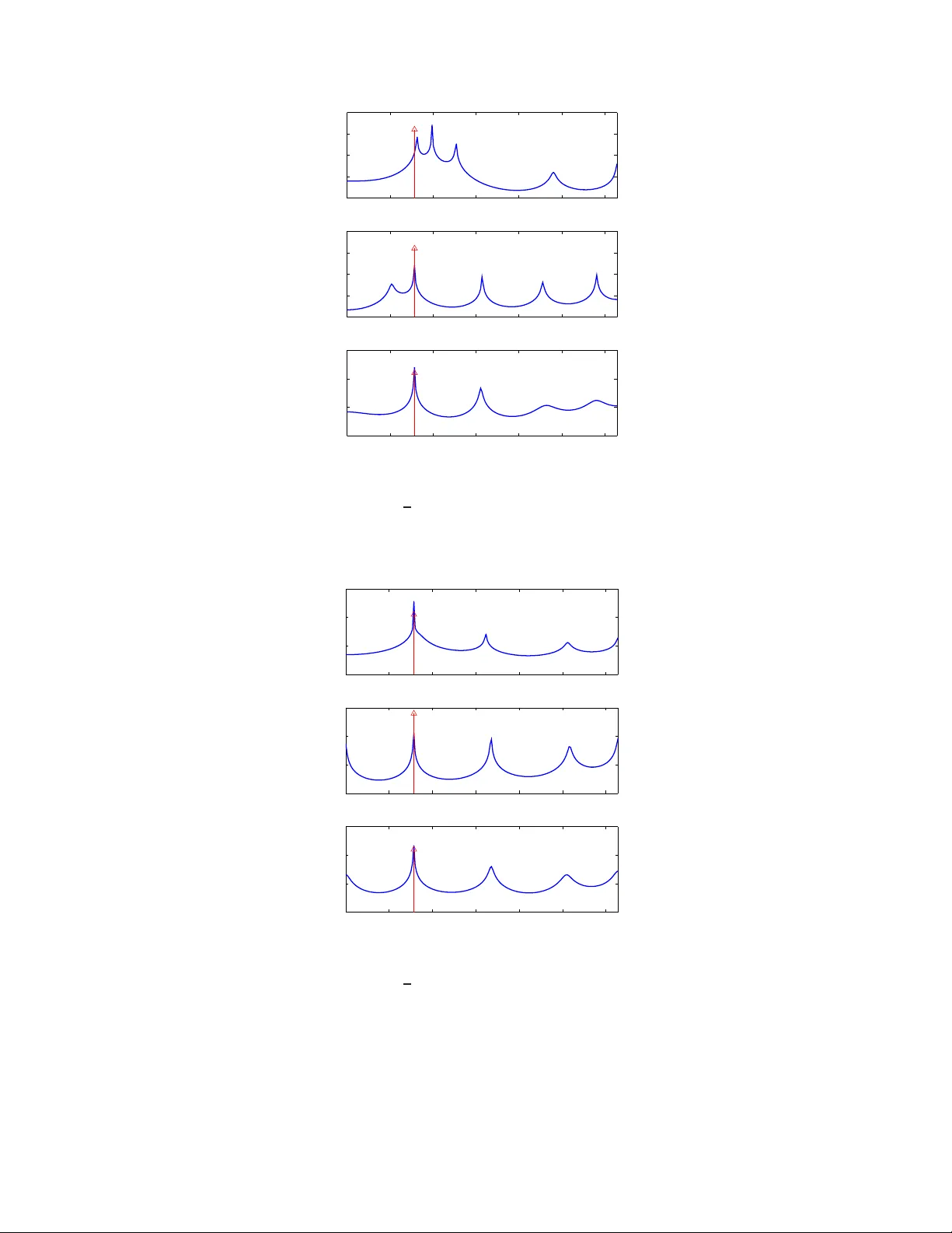
1 Geometric methods for estimat ion of structure d cov ariance s Lipeng Ning, Xianhua Jiang and Tryphon Geor giou Abstract W e consider p roblems of estimation of structur ed covariance ma trices, and in particular of matrices with a T oeplitz structure. W e follow a geom etric vie wpoint that is b ased on some suitab le notion of distance. T o th is end , we overview and co mpare several altern ati ves m etrics an d div ergence measures. W e advocate a specific one which represents the W asserstein distance between the cor respond ing Gaussians distributions and show that it coincid es with the so-called Bur es/Hellinger distance between covariance matrices as well. M ost importan tly , b esides the physically appe aling interpretatio n, compu tation o f th e metr ic req uires solving a lin ear matrix inequality (LMI). As a con sequence, com putations scale nicely for pro blems inv olving large covariance m atrices, a nd linear prior constraints on the cov ariance stru cture are easy to handle. W e compar e this tr ansportation/Bu r es/Hellinger m etric with the max imum likelihood and th e Burg method s as to their pe rforman ce with regard to estimation of power spectra with spectral lines o n a represen tati ve case study f rom the literature. 1 I . I N T RO D U C T I O N Consider a zero-mean , real-valued, discrete-time stationary random process { x ( t ) , t ∈ Z } . Let r ( t ) := E ( x ( k ) x ( k + t )) , with k , t ∈ Z , d enote the a utocorrelation function, and T :=      r 0 r 1 · · · r n − 1 r − 1 r 0 · · · r n − 2 . . . . . . . . . . . . r − ( n − 1) r − ( n − 2) . . . r 0      the covariance of the finite (obse rv ation) vector x =  x (0) , x (1) , . . . x ( n − 1)  ′ , i.e., T = E ( xx ′ ) . Th e covari ance ha s a T oep litz structure inherited by the ti me-in v ariance (stationarity) of the process . Through out, the size of such a n observation vector and of corres ponding finite T oep litz matrices will always be n and n × n , respe ctiv ely . The power spectrum of the process is unique ly determined by the (infinite) autoc orrelation function. This is due to the fact tha t the trigonometric moment p roblem is d etermined [1]. Then , sta rting with Bur g’ s e arly contributions [2], [3], mo dern non linear sp ectral an alysis technique s largely rely on a dmissible es timates of the pa rtial au tocorrelation sequen ce { r 0 , r 1 , . . . , r n − 1 } (equ i valently , of the T oeplitz covariance T ) from which information is so ught a bout correspond ing power s pectra. Admissibility o f the partial autoco rrelation sequen ce amo unts to the requirement that T is a positiv e se mi-definite matrix, in which case a positi ve se mi-definite extension to an infinite matrix is also possible. Part of the ch allenge, which was already addresse d b y Burg, is due to the fact that the s ample covari ance ˆ T := 1 m m X k =1 x k x ′ k , (1) where x k ( k ∈ { 1 , 2 , . . . , m } ) are inde pende nt observation vectors, may n ot be T oe plitz due to statistical errors. On the other han d, estimates of the ind i vidual entries { r 0 , r 1 , . . . , r n − 1 } via averaging over all av ailable s amples to 1 Dept. of Electrical & Comp. E ng., Univ ersity of Minnesota, Minneapolis, MN 55455. { ningx0 15, jiang082, tr yphon } @umn.edu. Supported in part by the NSF and AFOSR . 2 within a giv en time-distanc e from one an other , ma y not lea d to a pos iti ve matrix. Either way , the linea r structure or the positivit y is c ompromised. An early popular algorithm b y Burg aimed at ensuring positivity via a clever estimation of the so-called partial reflection coe f ficients instead of the autoco rrelation coef ficients (see e.g., [3]). Several alternative tricks were devised follo wed by a maximum likelihood ap proach in [4]. However , the issue was never put to res t beca use all these face challenge s of their own tha t lead to poo r resolution, bias, “line-sp liting” (where s inusoidal compon ents in the spectrum ge nerate ghos t peaks), and computa tional dif ficulties (as in the cas e of [4]). The so urce of the problem is lar gely the error in T which adversely affects our subs equen t estimate of the unde rlying power spec trum (obtained using e.g ., a Maximum Entropy method, the Capon e n v elope, etc.). Herein, we do no t ana lyze the problem of going from the T oeplitz c ov ariance to a power sp ectral estimate. Instead we focus only on the proble m of es timating the T o eplitz covariance from fi nite observations. The T oe plitz c ov ariance matrix is sou ght as the one closest to ˆ T in a suitable g eometry . Notions o f d istance from information theory , quan tum mechanics , and statistics lead to c omplementary viewpoints and so d oes maximum likelihood estimation of the autoco rrelation coe f ficients which also provides us with a no tion of distance . In Section II we outline the g eometric viewpoint togethe r with various possibilities for distanc e measu res. In Se ction III we discuss the respec ti ve o ptimization problems and in S ection IV we comp are the three most promising alternativ es on a specific exa mple from the literature. I I . G E O M E T R I C V I E W P O I N T Gi ven a sample covariance ma trix ˆ T , we con sider the problem to minimize min T ∈T d ( T , ˆ T ) , (2) over the c lass of admissible matrices T := { T : T ≥ 0 , T being T oeplitz } . In this, d represe nts a suitable notion of distanc e. V arious suc h d istance measu res are moti v ated below base d on s tatistics, information theory , qua ntum mechan ics, and o ptimal transportation. Occasiona lly , whe n the distance measure is n ot symmetric, we use the notation d ( T k ˆ T ) ins tead. Such no n-symmetric mea sures are often referred to as di ver gences in the literature. A. Likelihood dive r gence W e begin by disc ussing maximum likelihood estimation [4]. Assuming that the proce ss { x ( t ) , t ∈ Z } is Gauss ian, the joint density function for independe nt ob servation vectors x k ( k ∈ { 1 , 2 , . . . , m } ) is p ( X ; T ) = (2 π ) − mn 2 | T | − m 2 exp − 1 2 m X k =1 x ′ k T − 1 x k ! , with X := [ x 1 , . . . , x m ] . Then , ˆ T = 1 m XX ′ and the log -likeli hood function bec omes L ( ˆ T , T ) = log p ( X ; T ) = − m 2  n log (2 π ) + log | T | + trace( ˆ T T − 1 )  . (3) Thus, it is natural to see k a T oeplitz covariance matrix T for which L ( ˆ T , T ) is maximal. Note that if the x k ’ s are independ ent Ga ussian random variables, m ˆ T follows a W ishart distributi on. T hen (3) is the log-likelihood function of this distrib ution. Alternati vely , one may con sider the likelihood diver gence d L ( T || ˆ T ) := 1 m (log p ( x ; ˆ T ) − log p ( x ; T )) = 1 2 ( − log | ˆ T | + log | T | + trace( ˆ T T − 1 ) − n ) 3 as a relev ant n otion of distance s ince, evidently , d L ( T || ˆ T ) ≥ 0 , d L ( T || ˆ T ) = 0 ⇔ T = ˆ T . It relates to the Kullback-Leibler d i ver gence be tween correspon ding p df ’ s wh ich is discussed next. Howe ver , it does not define a me tric becau se it lac ks symmetry and may a lso fail to sa tisfy the triangular inequ ality . B. K ull back-Leibler dive r gence For rand om variables on R n with probability density functions p and ˆ p , the Kullback-Leibler (KL) di ver gence d KL ( p || ˆ p ) := Z R n p log  p ˆ p  dx (4) represents a well-accepted no tion of distance be tween the two [5], [6]. In the case where p an d ˆ p a re normal with zero-mean a nd covari ances T and ˆ T , res pectiv ely , their KL di ver gence become s d KL ( p || ˆ p ) = 1 2  log | ˆ T | − log | T | + trace( T ˆ T − 1 ) − n  , while d KL ( ˆ p || p ) = Z R n ˆ p log  ˆ p p  dx = 1 2 ( − log | ˆ T | + log | T | + trace( ˆ T T − 1 ) − n ) = d L ( T || ˆ T ) . C. F i sher metric and geodesic distance The KL di ver gence induc es a Riema nnian structure on the man ifold of p robability d istrib utions. The quadratic term o f d KL ( ˆ p || p + δ ) in the pe rturbation δ is the Fisher information me tric g p, Fisher ( δ ) = Z δ 2 p dx. (5) This turns out to be natural from one additional perspe ctiv e. It is the u nique Rieman nian me tric for which the stochas tic ma ps a re co ntracti ve [7] – a prop erty that motiv ates a rich family of me trics in the context of matricial counterparts o f p robability distrib utions (see below). For prob ability d istrib utions p ( x, θ ) parameterized by a vector θ the correspond ing metric is often referred to as Fisher-Rao [8] and giv en by g p, Fisher-Rao ( δ θ ) = δ ′ θ E  ∂ log p ∂ θ   ∂ log p ∂ θ  ′  δ θ . For zero-mean Gaus sian distributions parame terized b y co rresponding covariance matrices the metric b ecomes g T , Rao (∆) =    T − 1 / 2 ∆ T − 1 / 2    2 F (6) and is often na med a fter C.R. Rao . W e su mmarize this below . Throu ghout k M k F denotes the Frobenius norm p trace( M M ′ ) . Pr oposition 1: Conside r a zero-mean , normal distribution p with covariance T > 0 , a nd a perturbation p ǫ with covari ance T + ǫ ∆ . Provided || T − 1 / 2 ǫ ∆ T − 1 / 2 || F < 1 , d KL ( p || p ǫ ) = 1 4 g T , Rao ( ǫ ∆) + O ( ǫ 3 ) . Moreover , for δ = p ǫ − p , g T , Rao ( ǫ ∆) = 2g p, Fisher ( δ ) + O ( ǫ 4 ) . 4 The proof is giv en in Appen dix VI. The Fishe r- Rao metric has be en studied extensiv ely in rec ent yea rs [8], [9]. Geode sics and the g eodes ic distance on the respec ti ve Rieman nian manifolds can be c omputed explicitly . In fact, on the spac e of c ov ariance matrices, the geode sic distance b etween two p oints T and ˆ T is p recisely the log -deviation d Log ( T , ˆ T ) = k log ( ˆ T − 1 / 2 T ˆ T − 1 / 2 ) k F . T wo properties that are worth noting is that the metric is c ongruenc e in v ariant and that the correspon ding metric space is complete. D. Bur es metric and Bures/Hellinger distance As noted e arlier , the Fisher information metric is the uniqu e Riemannian metric for whic h stochastic maps are contracti ve. In quantum mechanics, a similar property has been s ought for the non-commutativ e analog of probability vectors, name ly , de nsity ma trices. Th ese are positiv e se mi-definite an d have trace equ al to one . In this setting, there are several metrics for which stocha stic map s (thes e a re now linear maps between sp aces of d ensity matrices, p reserving positivity a nd trac e) are contractive. They take the form trace(∆ D T (∆)) where D T (∆) can be thoug ht of as a “no n-commutativ e division” of the matrix ∆ by the matrix T . Th us, if T , ∆ are sca lars, the ab ove co llapses to ∆ 2 /T . Particular expressions g enerating su ch a “non-commu tati ve di vision” are D T , 1 (∆) := T − 1 ∆ , (7a) D T , 2 (∆) := Z ∞ 0 ( T + s I ) − 1 ∆( T + s I ) − 1 ds, (7b) D T , 3 (∆) := M , where 1 2 ( T M + M T ) = ∆ , (7c) see e .g., [10]. The metric correspon ding to (7a) w as stud ied by Petz [10], the metric correspon ding to (7b) is induced by the von Ne umann entropy on density matrices and is kn own as the Kubo-Mori metric [10 ], while (7c) giv es rise to the Bures metric. The Bures metric can also b e written as g T , Bures (∆) := min W { k Y k 2 F | ∆ = Y W ′ + W Y ′ , T = W W ′ } , see [11]. Acco rdingly , the c orresponding ge odesic distance on the manifold of de nsity matrices is called the Bures length. Assuming the normalization trace( T ) = 1 (i.e., that T ≥ 0 is a den sity matrix), k W k 2 F = 1 . Thus, we c an regard W as an e lement on a unit sphe re. Then, the Bu res leng th is the a rc length between c orresponding p oints on the sphere. The Bures metric has a close conne ction to the so-ca lled Hellinger distan ce. A ge neralization of the standard Hellinger distance to ma trices p roposed in F errante etal. [12 ] is d H ( T , ˆ T ) : = min U,V n k T 1 2 U − ˆ T 1 2 V k F | U U ′ = I , V V ′ = I o = min U n k T 1 2 U − ˆ T 1 2 k F | U U ′ = I o , (8) since, c learly , on ly one unitary transformation U can attain the sa me minimal value. This d if fers from the more s tan- dard way to ge neralize the scalar He llinger distance to matrices which is trace(( T 1 / 2 − ˆ T 1 / 2 ) 2 ) . The gene ralization in (8) is b etter k nown in qu antum mech anics literature as the Bures distance when the matrices are normalized to have trace 1 . It is se en that the Bures/Hellinger distance represen ts a “ straight line” distan ce b etween represe ntati ves of two “points” on the sphere as measured when imbedded in a linear Euc lidean space. The representatives amou nt to a selection o f suitable p oints o n an equiv alence class defined via un itary transformations. Interestingly , as shown in [11], [12], d H ( T , ˆ T ) =  trace( T + ˆ T − 2( ˆ T 1 2 T ˆ T 1 2 ) 1 2 )  1 2 . 5 Also, the optimizing unitary matrix U in (8) is U = T − 1 2 ˆ T − 1 2 ( ˆ T 1 2 T ˆ T 1 2 ) 1 2 . W e no te that the Hellinger distance applies equally well to pos iti ve definite matrices without any need to normalize T a nd ˆ T , and a s s uch, it h as been u sed to co mpare multi v ariate power sp ectral de nsities [12 ]. E. T rans portation distance W e shift to a seemingly different way of comparing p df ’ s. Th e transportation distance quan tifies the c ost for transferring o ne “mas s” distribution to an other ac counting for the comb ined cost of moving every unit o f mass from one loc ation to an other . Backgrou nd on transportation problems go es b ack to the work of G. Mong e in the 1700’ s. T he recent interes t was spa rked by the developments in the 194 0’ s by L. Kantorovich who is conside red the father of the s ubject 2 . The impo rtance of transportation distances in proba bility theo ry stems from the fact that the respec ti ve metrics are weakly continuou s. W e con sider distributi ons in R n and a quad ratic cost. A formulation of the Mon ge-Kantorovich transportation problem (with a qua dratic co st) directly in probab ilistic terms is as follo ws. Let X and Y be rando m variables in R n having pdf ’ s p x and p y . Determine d 2 W 2 ( p x , p y ) := inf p  E ( | X − Y | 2 ) | Z x p = p y , Z y p = p x  . (9) The metric d W 2 is known as the W asse rstein metric and, qu ite surprisingly , a lso induce s a Riemannian structure on probability densities [13], [14] – a rather deep re sult. Returning to the a bove op timization, the cost is s imply the minimum variance wh en the marginals of the joint distributi on are spe cified. W e now ass ume tha t T and ˆ T are the c ov ariances of X and Y , respectively , and we let S = E ( X Y ′ ) denote their c orrelation. Further , ass uming that their joint distrib ution is Gau ssian we obtain d 2 W 2 ( p, ˆ p ) = min S n trace( T + ˆ T − S − S ′ ) |  T S S ′ ˆ T  ≥ 0  . (10) A closed form solution is easy to o btain [15], [16]: S 0 = ˆ T − 1 2 ( ˆ T 1 2 T ˆ T 1 2 ) 1 2 ˆ T 1 2 , (11) and the trans portation distance is giv en alternativ ely by d W 2 ( p, ˆ p ) =  trace( T + ˆ T − 2( ˆ T 1 2 T ˆ T 1 2 ) 1 2 )  1 2 . Since this is cen tral to ou r the me, we provide de tails in Appen dix VII. Compa ring now with the c orresponding expression for the Hellinger distance we readily have the following. Pr oposition 2: For p an d ˆ p Gau ssian z ero me an d istrib utions with cov ariances T an d ˆ T , respectiv ely , d H ( T , ˆ T ) = d W 2 ( p, ˆ p ) . I I I . A P P RO X I M A T I O N O F S T RU C T U R E D C OV A R I A N C E S Returning to the structured covariance a pproximation problem, we co nsider the computa tion o f the optimizers for (2 ). W e do this for every choice o f d istance discus sed in the previous s ection. 2 L. Kantorovich received the Nobel prize in Economics in 1975 for his related work on mass transport and resource allocation. 6 A. Appr oximation base d on KL divergence and likelihood If we use d KL giv en in (4) as the distance between T a nd ˆ T , for the ap proximation problem we nee d to s olve min T ∈T n log | ˆ T | − log | T | + trace( T ˆ T − 1 ) − n o . (12) This is c on ve x in T , provided ˆ T > 0 , a nd he nce nu merically feasible. Howev er , the problem is v acuous whe n ˆ T is sing ular . This is un satisfactory sinc e the case when ˆ T is singular is important and quite c ommon. Alternatively , if we u se the likelihood diver gence d L ( T || ˆ T ) as distanc e me asure, the optimization prob lem min T ∈T n − log | ˆ T | + log | T | + trace( ˆ T T − 1 ) − n o (13) is well defined for s ingular ˆ T as well. A neces sary condition for a local minimum of (13) giv en in [4] is: trace  ( T − 1 ˆ T T − 1 − T − 1 ) Q  = 0 , (14) for all T oe plitz Q an d pointed ou t in [4] that, provided ˆ T is n ot s ingular , there is at least one local minimum o f (13) which is positiv e definite. Ba sed on this, Burg etal [4] giv e a numerical me thod to solve (13). The me thod is computationally demand ing a nd n umerically s ensitiv e, espe cially when ˆ T is s ingular . B. Appr oximation base d on log-deviation The optimization problem min T ∈T n k log ( ˆ T − 1 / 2 T ˆ T − 1 / 2 ) k F o . (15) is not con vex in T . Linearization of the objec ti ve func tion ab out ˆ T ma y b e us ed instead, s ince this leads to min T ∈T n k ˆ T − 1 / 2 T ˆ T − 1 / 2 − I k F o (16) which is a con vex problem. C. Based on Hellinger an d transp ortation distance Using d H ( T , ˆ T ) the relevant o ptimization problem (2) be comes min T ∈T n trace( T + ˆ T − 2( ˆ T 1 2 T ˆ T 1 2 ) 1 2 ) o . (17) At the outset, this a ppears dif ficult. Howe ver , from Prop osition 2 we know that d H ( T , ˆ T ) = d W 2 ( p, ˆ p ) . He nce, we may evaluate (17) via solving min T ∈T , S  trace( T + ˆ T − S − S ′ ) |  T S S ′ ˆ T  ≥ 0  . (18) This is n ow a semi-definite program a nd c an be solved quite e f ficiently [17]. The above expression for the transportation d istance can be given an alternative interpretation as follows. W e postulate the s tatistical mo del ˆ x = x + v where v repres ents noise, and ˆ T and T are the covariances of ˆ x an d x , resp ectiv ely . The covariance of x is known to be in the admissible set T while that of ˆ x may not, d ue to no ise. Thus, in the ab sence o f a dditional priors, it is reasona ble to see k an “ explanation” of the estimated covariance ˆ T by assuming the leas t possible amou nt of n oise. Allo wing for p ossible c oupling between x a nd v brings us to minimize E { v ′ v } = trace( T + ˆ T − S − S ′ ) subject to positiv e semi-definitene ss of the covariance of [ x ′ , ˆ x ′ ] ′ . This is precisely (18). 7 Analogous rationale, albeit with dif ferent a ssumptions has been use d to justify dif ferent methods . For instance, assuming that ˆ x = x + v whe re x an d v are indepen dent leads to min T ∈T n trace( ˆ T − T ) | ˆ T − T ≥ 0 o which is a method prop osed in [18 ]. Then, also, assu ming a “symmetric” noise c ontrib ution as in ˆ x + ˆ v = x + v , where the noise vectors ˆ v and v are ind epende nt of x and ˆ x , leads to min T ∈T ,Q, ˆ Q n trace( ˆ Q + Q ) | ˆ T + ˆ Q = T + Q, Q, ˆ Q ≥ 0 o , where ˆ Q and Q de signate c ov ariances of ˆ v a nd v , res pectively . Th e minimum in this ca se is the nuclear norm of ˆ T − T an d studied as a pos sibility in [19]. I V . E X A M P L E S W e no w c ompare how well two of the method s outlined earlier perform in identifying a single s pectral line in white noise and c ompare those with the stan dard Burg’ s method . W e choos e pa rameters as in the examp le in Burg etal. [4]. For constructing power spec tra co rresponding to a fin ite set of cov ariance samples and we use autoregressive models in order to be consiste nt with [4]. By using the same type of p ower s pectra we iso late and compare the e f fect of co rrecting for the “ non-T oeplitz-ness ” via ea ch of thes e two methods and by Burg’ s me thod. The data consists of a sinusoid (leading to a sing le sp ectral line) with three different p hase values and the same random vector for the noise. W e a ssume a single observation vector of size 11 , hence both x and v are vectors, and thus, the es timated covari ance ˆ T is (11 × 11) , sing ular , and of rank equal to 1 . Th us, the data is the sa me additiv e mixture of sinus oid and noise as in [4]: x ( t ) = cos( π 4 t + ψ ) + v ( t ) , t = 0 , 1 , . . . , 10 . The initial phase ψ is chose n for three diff erent values π 4 , π 2 and 3 π 4 . The noise vector v is fixed as v = [0 . 00 0562 , − 0 . 019127 , 0 . 007377 , − 0 . 00014 9 , − 0 . 00747 9 , − 0 . 013960 , 0 . 0035 10 , 0 . 0123 80 , 0 . 0069 79 , 0 . 0030 92 , 0 . 010053 ] ′ , generated from a zero-mean Gau ssian dis trib ution with vari ance 0 . 0001 . The first plot in Figure 1 s hows the power spec tral density (PSD) using Burg’ s me thod for estimating the partial correlation coefficients (as in [4]), while the secon d and third plots are based on covariances a pproximated us ing the likelihood-based method an d transportation-bas ed me thods, respec ti vely . The da ta correspo nds to ψ = π 4 and the res olution of the p lots is π 200 . Th e (red) arrow in the plots indicates the frequency of the s inusoidal compon ent. Burg’ s metho d s plits the spe ctral line into three. Th e s pectral line clos est to the true (red a rro w) is also significantly off . On the other hand, b oth, the likelihood-based and the transportation-based method s d etect the spe ctral line at the correct frequency (with relati vely ins ignificant error). Figure 2 shows the sa me s ituation but for ψ = π 2 . All three method s detec t the sp ectral line perfectly , to within the stated resolution. F igure 3 corresp onds to the cas e where ψ = 3 π 4 . Burg’ s method co nsistently splits the true spectral line into two n earby ones. The likelihood-based method gives a sma ll peak ne ar the true s pectral line, although the d ominant line is loc ated at the true frequ ency to within the stated res olution. On the other hand, the transportation-based method gives a result wh ich is consistent with the previous two situations . For the p urpose of detecting line spectra, the transportation-based method ap pears to be the mos t robust. A poten tial drawbac k of the transpo rtation-based metho d is that it giv es a bias ed estimate for the en ergy in the sinusoidal c omponen t. This is typically s maller than the true value in the example. 8 0 0.5 1 1.5 2 2.5 3 0 0.5 1 1.5 2 2.5 3 0 0.5 1 1.5 2 2.5 3 Fig. 1. Est imated maximum entropy spectrum for ψ = π 4 : i) Burg’ s method, ii ) Maximum likelihood method, i ii) Minimum transportation method. 0 0.5 1 1.5 2 2.5 3 0 0.5 1 1.5 2 2.5 3 0 0.5 1 1.5 2 2.5 3 Fig. 2. Est imated maximum entropy spectrum for ψ = π 2 : i) Burg’ s method, ii ) Maximum likelihood method, i ii) Minimum transportation method. V . R E C A P Most mod ern spectral analys is method s rely on estimated covari ance statistics. Y et, they are sens iti ve to those statistics a biding by the requisite linear structure, e .g., T oeplitz. In this pap er we discusse d and c ompared two of the most promising methods for approximating a sample covariance with one of the required structure. Contributions in the pape r inc lude drawing the co nnection between approximation in the Hellinger distan ce a nd approximation 9 0 0.5 1 1.5 2 2.5 3 0 0.5 1 1.5 2 2.5 3 0 0.5 1 1.5 2 2.5 3 Fig. 3. Esti mated maximum entropy spectrum for ψ = 3 π 4 : i) B urg’ s method, ii) Maximum likelihood method, iii ) Minimum transportation method. in the s ense of o ptimal mass transport. The latter can be c ast as a semidefinite p rogram wh ich is ea sy to solve and impervious to possible s ingularity or near-singularity of the sample covariance. The issue wit h the sa mple cov ariance ˆ T be ing s ingular is often neglected in estimation problems. Y e t, it is ubiquitous when only few s hort observation reco rds are av ailable —a situation which is c ommon in the ana lysis of n on-stationary processes . Furthermore, the u niquenes s and o ther properties of a maximum likelihood estimate, when ˆ T is singu lar , are not well und erstood [4]. As a fi nal remark we note tha t interest in other linea r structures for covariance ma trices, bes ides that of T oeplitz, arises whe n the vectorial proces s is the state vector of a linear s ystem. In such a case , T satisfies linear con straints that in v olve the system dyn amics [20]. All ea rlier disc ussion and methods ca n be repeated verbatim for the problem of approximating sample s tate-covari ances. V I . A P P E N D I X A : P RO O F F O R T H E P RO P O S I T I O N 1 The KL d i ver gence b etween a ze ro-mean normal distribution p with covariance T > 0 and a p erturbation p ǫ with covari ance T + ǫ ∆ is d KL ( p || p ǫ ) = 1 2  log det( T + ǫ ∆) − log det( T ) + trace  ( T + ǫ ∆ ) − 1 T  − n  . Define ∆ T = T − 1 / 2 ∆ T − 1 / 2 , then d KL ( p || p ǫ ) = 1 2  log det  T 1 / 2 ( I + ǫ ∆ T ) T 1 / 2  − log d et( T ) + trace  T − 1 / 2 ( I + ǫ ∆ T ) − 1 T − 1 / 2 T  − n  = 1 2  log det( I + ǫ ∆ T ) + trace( I + ǫ ∆ T ) − 1 − n  . (19) W e expand ( I + ǫ ∆ T ) − 1 into the T aylor series ( I + ǫ ∆ T ) − 1 = I − ǫ ∆ T + ǫ 2 ∆ T 2 − ǫ 3 ∆ T 3 + · · · . (20) 10 Let λ i , i = 1 , · · · , n , represe nt eigenv alues of ∆ T , then log det( I + ǫ ∆ T ) = n X i =1 log(1 + ǫλ i ) = n X i =1 ( ǫλ i − 1 2 ǫ 2 λ 2 i + 1 3 ǫ 3 λ 3 i + · · · ) = ǫ trace(∆ T ) − 1 2 ǫ 2 trace(∆ T 2 ) + 1 3 ǫ 3 trace(∆ T 3 ) + · · · . (21) W e sub stitute (20) a nd (21) into (19) to ob tain d KL ( p || p ǫ ) = 1 4 ǫ 2 trace(∆ T 2 ) + O ( ǫ 3 ) . By a similar computation, one ca n eas ily see that d KL ( p ǫ || p ) g i ves rise to the sa me metric, thou gh the coefficients of higher o rder terms on ǫ are different from thos e c orresponding to d KL ( p || p ǫ ) . T o draw a conne ction with the Fisher metric, we subs titute δ = p ǫ − p into the Fish er metric: g p, Fisher ( δ ) =  Z R n det( T ) 1 / 2 (2 π ) n/ 2 det( T + ǫ ∆) e − 1 2 y ′ (2( T + ǫ ∆) − 1 − T − 1 ) y dy − 1  . Since || ǫ ∆ T || F < 1 , ǫ 2 ∆ T 2 < I and henc e − I < ǫ ∆ T < I . Multiplying b y T 1 / 2 from left and right on all s ides of the above ine quality , we obtain − T < ǫ ∆ < T , or equiv alently 0 < 1 2 T + 1 2 ǫ ∆ < T . It follo ws that − ( 1 2 T + 1 2 ǫ ∆) − 1 < − T − 1 , or equiv alently , 2( T + ǫ ∆) − 1 − T − 1 > 0 . Consequ ently 1 (2 π ) n/ 2 det (2( T + ǫ ∆) − 1 − T − 1 ) − 1 / 2 e − 1 2 y ′ (2( T + ǫ ∆) − 1 − T − 1 ) y is a Gau ssian distributi on with mean 0 and c ov ariance (2( T + ǫ ∆) − 1 − T − 1 ) − 1 . Since the integral of a Gau ssian distrib ution is 1 , w e obtain that g p, Fisher ( δ ) = det( T ) 1 / 2 det (2( T + ǫ ∆) − 1 − T − 1 ) 1 / 2 det( T + ǫ ∆) − 1 ! . But ( T + ǫ ∆) − 1 = T − 1 / 2 ( I + ǫ ∆ T ) − 1 T − 1 / 2 , and 2( T + ǫ ∆) − 1 − T − 1 = T − 1 / 2  2( I + ǫ ∆ T ) − 1 − I  T − 1 / 2 . Consequ ently , det  2( T + ǫ ∆) − 1 − T − 1  1 / 2 det( T + ǫ ∆) = det  ( T + ǫ ∆ )  2( T + ǫ ∆) − 1 − T − 1  ( T + ǫ ∆)  1 / 2 = det  T 1 / 2 ( I + ǫ ∆ T )  2( I + ǫ ∆ T ) − 1 − I  ( I + ǫ ∆ T ) T 1 / 2  1 / 2 = det( T ) 1 / 2 det( I − ǫ 2 ∆ T 2 ) 1 / 2 , 11 and g p, Fisher ,m ( δ ) =  det( I − ǫ 2 ∆ T 2 ) − 1 / 2 − 1  =  det( I + ǫ 2 ∆ T 2 + ǫ 4 ∆ T 4 + · · · ) 1 / 2 − 1  . Once again c onsidering the eigen v alues o f ∆ T we g et det( I + ǫ 2 ∆ T 2 + ǫ 4 ∆ T 4 + · · · ) 1 / 2 = n Y k =1 ( ∞ X i =0 ( ǫλ k ) 2 i ) ! 1 / 2 =   1 + n X k =1 ǫ 2 λ 2 k + X k ≤ l ǫ 4 λ 2 k λ 2 l + · · ·   1 / 2 = 1 + 1 2 ǫ 2 k ∆ T k 2 F + O ( ǫ 4 ) , where in the last e quality we have use d the fact that n P k =1 λ 2 k = trace(∆ T 2 ) = k ∆ T k 2 F . The refore, g p, Fisher ( δ ) = 1 2 g T , Rao (∆) + O ( ǫ 4 ) . V I I . A P P E N D I X B W e n ow s how that given two n × n matrices T > 0 an d ˆ T > 0 , arg min S  trace( T + ˆ T − S − S ′ ) |  T S S ′ ˆ T  ≥ 0  has indeed the explicit closed -form expression S 0 = ˆ T − 1 2 ( ˆ T 1 2 T ˆ T 1 2 ) 1 2 ˆ T 1 2 , (22) Consider the Shur complement P := T − S ˆ T − 1 S ′ which is clearly no nnegativ e definite. Then , S ˆ T − 1 2 = ( T − P ) 1 2 U , whe re U U ′ = I , and S = ( T − P ) 1 2 U ˆ T 1 2 . (23) Moreover , trace( S ) = trace(( T − P ) 1 2 U ˆ T 1 2 ) = trace( ˆ T 1 2 ( T − P ) 1 2 U ) . (24) Since T and ˆ T are g i ven, minimizing trace( T + ˆ T − S − S ′ ) is the same as ma ximizing trace( S ) . Let U S Λ S V ′ S be the singular value de compos ition o f ˆ T 1 2 ( T − P ) 1 2 , and U 0 := arg max U { trace( ˆ T 1 2 ( T − P ) 1 2 U ) | U U ′ = I } . Then, U 0 must satisfy V ′ S U 0 = U ′ S and ˆ T 1 2 ( T − P ) 1 2 U 0 = ( ˆ T 1 2 ( T − P ) ˆ T 1 2 ) 1 2 . (25) From (24) we have trace( S ) = trace (( ˆ T 1 2 ( T − P ) ˆ T 1 2 ) 1 2 ) . Since P ≥ 0 , the trace( S ) is maximal whe n P = 0 . Moreover , if P = 0 , rank  T S S ′ ˆ T  ≤ rank( T ) , and ˆ T = S ′ 0 T − 1 S 0 . Thus, setting P = 0 into (25), we have U 0 = T − 1 2 ˆ T − 1 2 ( ˆ T 1 2 T ˆ T 1 2 ) 1 2 , and conse quently S 0 = ˆ T − 1 2 ( ˆ T 1 2 T ˆ T 1 2 ) 1 2 ˆ T 1 2 . 12 R E F E R E N C E S [1] U. Grenande r and G. Szeg ¨ o, T oeplitz F orms and their Applications . Chelsea Pub Co, 2001. [2] J. B urg, “Maximum entropy spectral analysis, ” Ph.D. dissertati on, Stanford Univ ersity , S tanford, CA, 1975. [3] S. Haykin, Nonlinear Methods of Spectral Analysis . Springer-V erlag, 1979. [4] J. Burg, D. Luenber ger , and D. W enger , “Estimation of structured cov ariance matrices, ” Pr oceeding s of the IEE E , vo l. 70, no. 9, pp. 963–97 4, 1982. [5] S. Kullback and R. A. Leibler, “On information and sufficienc y , ” The A nnals of Mathematical Statistics , vol. 22, no. 1, pp. 79–86, 1951. [6] T . Cov er and J. T homas, Elements of Information Theory . Wile y-Interscience, 2008. [7] N. Cenco v , Statistical Decision Rules and Optimal Inferen ce . Amer . Math. Soc., 1982, no. 53. [8] S.-I. Amari, “Differential-geometrical methods i n statistics, ” Lecture Notes in Statistics , vol. 28, 1985. [9] R. Bhatia, P ositive Definite Matrices . Princeton University Press, 2007. [10] D. Petz, “Geometry of canonical correlation on the state space of a quantum system, ” Journa l of Mathematical Physics , vol. 35, pp. 780–79 5, 1994. [11] A. Uhlmann, “The metric of B ures and the geometric phase, ” Quantum Gr oups and Related T opics , pp. 267–264 , 1992. [12] A. Ferrante, M. Pav on, and F . R amponi, “Hellinger versus Kullback–Leibler multiv ariab le spectrum approximation, ” Automatic C ontr ol, IEEE T ransa ctions on , vol. 53, no. 4, pp. 954–967, 2008. [13] J. Benamou and Y . Brenier , “ A computational fl uid mechanics solution to the Monge-Kantorovich mass transfer problem, ” Numerische Mathematik , vol. 84, no. 3, pp. 375–393, 2000. [14] R. Jordan, D. Kinderlehrer , and F . Otto, “The variational formulation of the Fokke r-Planck equation, ” SIAM journal on mathematical analysis , vol. 29, no. 1, pp. 1–17, 1998. [15] I. Ol kin and F . Pukelsheim, “The distance between two random vectors with giv en dispersion matrices, ” L inear Algebra and its Applications , vol. 48, pp. 257–263, 1982. [16] M. Knott and C . S. Smit h, “On the optimal mapping of distributions, ” Journa l of Optimization Theory and Applications , vol. 43, no. 1, pp. 39–49, 1984. [17] S. Boy d and L. V andenb erghe, Conve x Optimization . Cambridge University P ress, 2004. [18] P . Stoica, L. Du, J. Li, and T . Georgiou, “ A new method for moving-a v erage parameter estimation, ” in Confer ence R ecor d of the F orty F ourth Asilomar Confer ence on Signals, Systems and Computer s , 2010, pp. 1817– 1820. [19] T . Georgiou, “Distances between time-series and their autocorrelation statistics, ” Modeling, Esti mation and Control , pp. 113–122 , 2007. [20] ——, “The structure of state cov ariances and its relation to the power spectrum of the input, ” Automatic Contr ol, IEEE T ra nsactions on , vol. 47(7), pp. 1056–1066, 2002.