Bayesian Post-Processor and other Enhancements of Subset Simulation for Estimating Failure Probabilities in High Dimensions

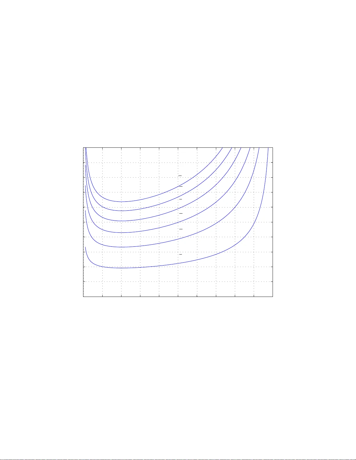
Ba y esian P ost-Pro cessor and other Enhancemen ts of Subset Sim ulation for Estimating F ailure Probabilitie s in High Dimensions Konstan tin M. Zuev 1 , James L. Bec k 1 , Siu-Kui Au 2 , Lam bros S. K atafygiotis 3 Abstract Estimation of small failure p robabilities is one of the most imp ortan t and chal - lenging computational p roblems in reliabilit y engineering. The failure pr ob ab ility is us u ally giv en b y an in tegral o ve r a h igh-dimensional uncertain p arameter space that is difficult to ev aluate numerically . This pap er fo cuses on enhancemen ts to Subset S imulation (SS), prop osed b y Au and Bec k, wh ic h pro vides an efficient al- gorithm b ased on MCMC (Mark ov c hain Monte C arlo) sim ulation for computing small f ailure probabilities for general high-dimensional reliabilit y problems. First, w e analyze the Modified Metrop olis algorithm (MMA), an M CMC tec hn iqu e, which is used i n SS for sampling from high-dimensional conditional d istributions. The effi- ciency and ac cur acy of SS directly dep ends on the ergo dic prop erties of the Marko v c hains generated by MMA, wh ic h con trol how fast the c h ain explores the parameter space. W e presen t some observ ations on the optimal scaling of MMA for efficien t exploration, and dev elop an optimal scaling strategy for this algorithm w hen it is emplo y ed within SS. Next, w e p r o vide a theoretical basis for the optimal v alue of the conditional fail u re probabilit y p 0 , an imp ortant p arameter on e has to c ho ose when using SS. W e demonstrate that choosing an y p 0 ∈ [0 . 1 , 0 . 3] will give similar efficiency as the optimal v alue of p 0 . Finally , a Ba ye sian p ost-pro cessor SS+ for the original S S metho d is dev elop ed where the uncertain f ailur e pr obabilit y that one is estimating is mo d eled as a stochastic v ariable wh ose p ossible v alues b elong to the unit interv a l. Sim ulated samples from SS are view ed as in f ormativ e data relev an t to the system’s reliabilit y . I n stead of a sin gle r eal n umb er as an estimate, SS+ pro- duces the p osterior PDF of the fai lu re probabilit y , wh ic h tak es in to accoun t b oth prior inf ormation and the information in the samp led data. Th is PDF qu an tifies the uncertaint y in the v alue of the fail u re probability and i t ma y b e further used in r isk analyses to incorp orate this un certaint y . T o demonstrate S S+, w e consider its application to tw o different r eliabilit y problems: a linear r eliabilit y p r oblem and reliabilit y analysis of an elasto-plasti c str u cture sub j ected to strong seismic ground motion. The relationship b et w een the original SS and SS + is also discuss ed. KEY WORDS: Rare Ev en t Sim ulation; Sto chastic Sim ulation Metho ds; Mark ov c hain Mon te Carlo; Subset Simulation; Ba yes ian Approac h. 1 Division of Engineering and Applied Science, California Institute of T echnology , Mail C o de 10 4 -44, Pasadena, CA 91 125, USA (Emails: zuev@caltech.edu, jimbeck@caltech.edu) 2 Department o f Building and Construction, City Univ ersity of Hong Kong, 83 T at Chee Av enue, Kowloon, Ho ng Ko ng (Email: siukuiau@cit y u.e du.hk) 3 Department o f Civil and En vir onmental Engineer ing, The Hong Kong Universit y of Science and T echnology , Hong Kong , China (Email: lam bros @ust.hk) 1 1 In tro duction One of the most important and c hallenging problems in reliabilit y engineering is to es- timate the failure probability p F for a system, that is, the probabilit y of unacceptable system p erformance. This is usually expresse d as an in tegral ov er a high-dimensional uncertain parameter space: p F = Z I F ( θ ) π ( θ ) dθ = E π [ I F ( θ )] , (1) where θ ∈ R d represen ts the uncertain parameters needed to sp ecify completely the ex- citation and dynamic mo del of the system; π ( θ ) is the join t probability densit y function (PDF) fo r θ ; F ⊂ R d is the failure domain in the parameter space (i.e. the set of parame- ter v alues that lead to p erformance of the system that is considered to b e unacceptable); and I F ( θ ) stands for the indicator function, i.e. I F ( θ ) = 1 if θ ∈ F and I F ( θ ) = 0 if θ / ∈ F . The dimension d is t ypically large for dynamic r eliability problems (e.g. d ∼ 10 3 ) b ecause the sto c hastic input time histor y is discretized in time. As a result, the usual n umerical quadrature metho ds for integrals are not computationally feasible fo r ev aluation (1). Ov er the past decade, the engineering researc h communit y has realized the imp ortance of adv a nced sto chastic sim ulation methods f or reliabilit y analysis. As a result, many differen t efficien t algorithms ha ve b een dev elop ed recen tly , e.g. Subset Sim ulat io n [2 ], Imp ortance Sampling using Elemen tary Ev en ts [3], Line Sampling [28], Auxiliary domain metho d [25 ], Spherical Subset Sim ulatio n [24], Horseracing Sim ulation [44], to name but a few. This pap er fo cuses on enhancemen ts to Subset Sim ulatio n (SS), prop osed b y Au and Bec k in [2], whic h pro vides an efficien t algorithm for computing failure probabilities for general hig h- dimensional reliabilit y problems. It has b een show n theoretically [2 ] and v erified with different num erical ex amples (e.g. [4, 5, 39]) that SS giv es mu ch higher computational efficiency than standard Monte Carlo Sim ulation when estimating small failure probabilities. Recen tly , v arious mo difications of SS ha v e b een prop o sed: SS with splitting [9], Hybrid SS [10], and Tw o-Sta ge SS [23 ]. It is imp orta n t to highligh t, how ever, that no ne o f these mo difications offer a drastic impro v emen t ov er the original algorit hm. W e start with the analysis of the Mo dified Metrop olis algorithm (MMA), a Mark ov c hain Mon te Carlo techniq ue used in SS, which is presen ted in Section 2. The efficiency and accuracy of SS directly dep ends on the ergo dic prop erties of the Marko v c hains generated b y MMA. In Section 3, w e examine the optimal scaling of MMA to tune the parameters of t he algorithm to mak e the resulting Mark ov c hain con ve rg e t o stationarity as fast as p ossible. W e presen t a collection of observ a tions on the optimal scaling of MMA for different n umerical examples, and dev elop an optimal scaling strategy for MMA when it is emplo y ed within SS for estimating small f ailure probabilities. One of t he most imp ortan t comp onents of SS whic h affects its efficiency is the c hoice of the sequence of in termediate threshold v alues or, equiv alen tly , the in termediate failure probabilities (see Section 2, whe re the original SS algorithm is describ ed). In Section 4, a metho d for optimally c ho osing t hese probabilities is presen ted. The usual in terpretation of Mon te Carlo metho ds is consisten t with a purely fr e quen- tist approac h, meaning that they can b e in terpreted in terms of the f requen tist definition of probabilit y whic h identifies it with the long-run relativ e frequency of o ccurrence of an eve nt. An alternativ e in terpretation can b e made based on the Bayesia n approac h 2 whic h views pro ba bility as a measure of the plausibilit y of a prop osition conditional on incomplete information that do es not allow us to establish the truth or fa lseho o d of the prop osition with certaint y . Ba ye sian probabilit y theory w as, in fact, primarily deve lop ed b y the mathematician and astronomer Laplace [29, 30] for statistical analysis o f astro- nomical observ at io ns. Mor eov er, Laplace dev elop ed the w ell-known Ba y es’ theorem in full generalit y , while Ba y es did it only fo r a sp ecial case [6]. A complete dev elopmen t based on Laplace’s theory , with n umerous examples of its a pplications, was giv en b y the mathe- matician and geophy sicist Jeffreys [2 2] in the early 20 th cen tury . Despite its usefulness in applications, the w ork of Lapla ce and Jeffreys on probability w a s r ejected in fav or of the frequen tist approach by most statisticians un til la te last cen tury . Because of the absence of a strong rationale b ehind the theory at that time, it w as perceiv ed as sub jectiv e and not rigor ous by man y statisticians. A rig o rous lo g ic foundation for the Bay esian approa c h w as giv en in the seminal w ork of the phys icist Co x [11, 12] and expounded b y the ph ysi- cist Ja ynes [20, 21], enhancing Bay esian probabilit y theory as a con ve nient mat hematical language for inference and uncertain ty quan tification. Although the Bay esian a ppro ac h usually leads to high-dimensional in tegrals that of t en cannot b e ev aluated analytically nor n umerically by straig h tforward quadrature, the deve lopment of Marko v c hain Mon te Carlo algorithms and increasing computing pow er hav e led ov er the past few decades to an explosiv e growth of Bay esian pap ers in all researc h disciplines. In Section 5 of this paper, a Ba y esian p ost-pro cessor for the original Subset Sim ula- tion metho d is dev elop ed, where the uncertain failure probability that one is estimating is mo deled as a sto c hastic v ariable whose p ossible v alues b elong to the unit in terv al. Al- though this f a ilure probability is a constant defined by the in tegral in (1 ), its exact v alue is unkno wn b ecause the integral cannot b e ev aluated; inste ad, w e m ust infer it s v alue from av a ilable relev ant information. Instead of a single real n um b er as an estimate, the p ost-pro cessor, written as SS+ (“SS- plus”) f or short, pro duces the p osterior PDF of the failure probability , whic h tak es in to accoun t both rele v an t prior info rmation and the in- formation from the samples generated b y SS. This PDF expresse s the relativ e plausibilit y of each p ossible v alue of the failure probability based on this informat io n. Since this PDF quan tifies the uncertaint y in the v alue of p F , it can b e fully used in risk analyses (e.g. for life-cycle cost analysis, decision making under risk, etc.), or it can b e used t o giv e a p oint estimate suc h a s the most pr o bable v alue based on the av ailable information. 2 Subset Sim ulation 2.1 Basic idea of Subset Sim ulation The original and b est kno wn sto c hastic sim ulation algorithm for estimating high-dimensional in tegrals is Mon te Carlo Simu lat ion (MCS). In this method the failure probability p F is estimated b y approximating the mean of I F ( θ ) in (1) by its sample mean: p F ≈ ˆ p M C F = 1 N N X i =1 I F ( θ ( i ) ) , (2) where sample s θ (1) , . . . , θ ( N ) are independen t and iden tically distributed (i.i.d.) samples from π ( · ), denoted θ ( i ) i.i.d. ∼ π ( · ). This estimate is just t he fra ction o f samples that pro duce 3 system failure according to a mo del of the system dynamics. Notice that eac h ev a lua tion of I F requires a deterministic system analysis to b e p erformed to c hec k whether the sample implies failure. The main adv a n tage of MCS is that its efficiency do es not dep end on the dimension d o f the parameter space. Indeed, straig htforw ard calculation s hows that the co efficien t of v ariat ion (c.o.v) of the Mon te Carlo estimate (2), servin g as a measure of accuracy in the usual in terpretatio n of MCS, is giv en b y: δ ( ˆ p M C F ) = r 1 − p F N p F . (3) Ho w ev er, MCS has a serious dr awbac k: it is inefficien t in estimating small failure proba- bilities. If p F is v ery small, p F ≪ 1, t hen it fo llo ws fro m (3) that the n um b er of samples N (o r, equiv a len tly , num b er of system a nalyses) needed to a chiev e an acceptable leve l of accuracy is v ery large, N ∝ 1 /p F ≫ 1. This defic iency of M CS has motiv a ted res earch to de velop m or e efficien t sto chastic sim ulation alg orithms f o r e stimating small failure probabilities in high-dimensions. The basic idea of Subset Sim ulation [2] is the following: represen t a v ery small f a ilure probabilit y p F as a pro duct of larger probabilities so p F = Q m j =1 p j , where t he fa ctors p j are estimated sequen tially , p j ≈ ˆ p j , t o obtain an estimate ˆ p S S F for p F as ˆ p S S F = Q m j =1 ˆ p j . T o reac h this goal, let us consider a decreasing sequence of nested subsets of the par ameter space, starting from the en tire space and shrinking to the failure domain F : R d = F 0 ⊃ F 1 ⊃ . . . ⊃ F m − 1 ⊃ F m = F . (4) Subsets F 1 , . . . , F m − 1 are called interme d i a te failur e domai n s . As a result, the failure probabilit y p F = P ( F ) can b e rewritten as a pro duct of conditional probabilities: p F = m Y j =1 P ( F j | F j − 1 ) = m Y j =1 p j , (5) where p j = P ( F j | F j − 1 ) is the conditional probability at the ( j − 1) th conditional level. Clearly , by c ho osing the in termediate fa ilure domains appropriately , all conditional prob- abilities p j can b e made large. F urthermore, they can b e estimated, in principle, b y the fraction o f indep enden t conditional samples tha t cause fa ilure at the in termediate lev el: p j ≈ ˆ p M C j = 1 N N X i =1 I F j ( θ ( i ) j − 1 ) , θ ( i ) j − 1 i.i.d. ∼ π ( · | F j − 1 ) . (6) Hence, the original problem (estimation of the small failure probabilit y p F ) is replaced b y a sequence of m in termediate problems (estimation of the larger fa ilure probabilities p j , j = 1 , . . . , m ). The first probability p 1 = P ( F 1 | F 0 ) = P ( F 1 ) is straig h tforward to estimate b y M CS, since (6) requires sampling from π ( · ) that is assumed to b e readily sampled. Ho wev er, if j ≥ 2, to estimate p j using (6) one needs to generate indep enden t samples from conditional distribution π ( ·| F j − 1 ), whic h, in general, is not a trivial task. It is no t efficien t to use MCS for this purp ose, es p ecially at higher lev els, but it can b e done by a s p ecifically tailored Mark o v c hain Monte Carlo tec hnique at the exp ense of generating dep enden t samples. Mark o v c hain Monte Carlo ( MCMC) [3 1, 34, 35] is a class of algo rithms for sampling from m ulti- dimensional target probabilit y distributions that cannot b e directly sampled, 4 at least not efficien t ly . These metho ds a re based on constructing a Marko v chain that has the distribution of in terest as its stationary distribution. By sim ulating samples fr o m the Mark ov chain, they will eve ntually b e draws from t he target probability distribution but t hey will not b e indep enden t samples. In Subset Sim ulation, the Mo dified Metrop olis algorithm (MMA) [2], an MCMC tec hnique based on the orig ina l Metrop o lis algorithm [33, 1 8], is used f o r sampling from t he conditio na l distributions π ( ·| F j − 1 ). R ema rk 1 . It w as observ ed in [2] that the original Metropolis algorit hm do es not w ork in high-dimensional c onditio nal probabilit y spaces, b ecause it pro duces a Mark o v chain with very highly correlated states. The g eometrical r easons fo r this are discussed in [26]. 2.2 Mo d ified Metrop olis algorithm Supp ose w e wan t to generate a Mark ov chain with stationa r y distribution π ( θ | F ) = π ( θ ) I F ( θ ) P ( F ) = Q d k =1 π k ( θ k ) I F ( θ ) P ( F ) , (7) where F ⊂ R d is a subset of the parameter space. Without significan t loss o f generality , w e assume here that π ( θ ) = Q d k =1 π k ( θ k ), i.e. comp onen ts of θ a r e indep enden t (but are not so when conditioned on F ). MMA differs from the o riginal Metrop olis algorithm algorithm in the wa y t he candidate state ξ = ( ξ 1 , . . . , ξ d ) is generated. Instead of using a d -v ariate pro p osal PDF on R d to directly obtain the candidate state, in MMA a sequence of univ ariate prop osal PDFs is used. Namely , each co o rdinate ξ k of the candidate state is generated separately using a univ ariate prop osal distribution dep endent on the co ordinate θ k of t he current state. Then a ch eck is made whether the d - v ariate candidate generated in suc h a w ay b elongs to the subset F in whic h case it is accepted as the next Mark o v c hain state; otherwise it is rejected and the curren t MCMC sample is rep eated. T o summarize, the Mo dified Metrop olis a lgorithm pro ceeds as fo llo ws: Mo dified Metropo lis algorithm [2] Input: ⊲ θ (1) ∈ F , initial state o f a Mark ov c hain; ⊲ N , tota l num b er of states, i.e. samples; ⊲ π 1 ( · ) , . . . , π d ( · ), marginal PDFs of θ 1 , . . . , θ d , resp ectiv ely; ⊲ S 1 ( ·| α ) , . . . , S d ( ·| α ) , univ ariat e pro p osal PDFs dep ending on a par a meter α ∈ R and satisfying the symmetry prop ert y S k ( β | α ) = S k ( α | β ) , k = 1 , . . . , d . Algorithm: for i = 1 , . . . , N − 1 do % Generate a candidate state ξ : for k = 1 , . . . , d do Sample ˜ ξ k ∼ S k ( ·| θ ( i ) k ) Compute the acceptance ratio r = π k ( ˜ ξ k ) π k ( θ ( i ) k ) (8) Accept or reject ˜ ξ k b y setting ξ k =  ˜ ξ k , with pr o babilit y min { 1 , r } ; θ ( i ) k with pr o babilit y 1 − min { 1 , r } . (9) 5 end f or Chec k whether ξ ∈ F b y system analysis and accept or reject ξ b y setting θ ( i +1) =  ξ , if ξ ∈ F ; θ ( i ) , if ξ / ∈ F . (10) end f or Output: ◮ θ (1) , . . . , θ ( N ) , N states of a Marko v c hain with stationary distribution π ( ·| F ). Sc hematically , the Mo dified Metrop o lis algo rithm is sho wn in Figure 1. F or complete- ness and the reader’s conv enience, the pro of that π ( · | F ) is the stationary distribution for the Mark ov c hain g enerated b y MMA is g iv en in the App endix. R ema rk 2 . The symmetry prop erty S k ( β | α ) = S k ( α | β ) do es not pla y a critical role. If S k do es not satisfy this prop ert y , b y replacing the “Metrop olis” ratio in (8 ) b y the “Metrop olis-Hastings” ratio r = π k ( ˜ ξ k ) S k ( θ ( i ) k | ˜ ξ k ) π k ( θ ( i ) k ) S k ( ˜ ξ k | θ ( i ) k ) , (11) w e obtain an MCMC algor ithm referred to as the Mo dified Metrop olis–Hastings alg orithm. Th us, if w e run the Mark o v c hain for s ufficien tly long (the burn-in p erio d), s ta rting from essen tially an y “seed” θ (1) ∈ F , then for large N the distribution of θ ( N ) will b e appro ximately π ( ·| F ). Note, how ev er, that in an y practical application it is ve ry difficult to c hec k whether the Mark ov c hain has reac hed its stationary distribution. If the seed θ (1) ∼ π ( ·| F ), then all states θ ( i ) will b e auto matically distributed a ccording to the target distribution, θ ( i ) ∼ π ( · | F ), since it is the stationary distribution for the Marko v c hain. This is called p erfe ct sampling [35] and Subs et Simulation has this prop erty b ecause of the w a y the seeds a re c hosen [2]. Let us assume no w that w e are give n a seed θ (1) j − 1 ∼ π ( ·| F j − 1 ), where j = 2 , . . . , m . Then, using MMA, w e can generate a Mark o v c hain with N states starting f r om this seed and construct an estimate fo r p j similar to ( 6), where MCS samples a r e replaced b y MCMC samples: p j ≈ ˆ p M C M C j = 1 N N X i =1 I F j ( θ ( i ) j − 1 ) , θ ( i ) j − 1 ∼ π ( ·| F j − 1 ) . (12) Note that all samples θ (1) j − 1 , . . . , θ ( N ) j − 1 in (12) are identically distributed in the stationa ry state of the Mark ov c hain, but are not indep enden t. Nev ertheless, t hese MCMC samples can b e used for statistical av eraging as if they w ere i.i.d., although with some reduction in efficiency [14 ]. Namely , the more correlated θ (1) j − 1 , . . . , θ ( N ) j − 1 are, the le ss efficien t is the estimate ( 1 2). The correlatio n b et w een success ive samples is due to prop osal P D Fs S k , whic h gov ern t he generation of the next state of the Mark ov chain f r o m the curren t o ne in MMA. Hence, the c hoice o f prop osal PDFs S k con trols the efficiency of estimate (12), making this c hoice v ery imp ortan t. It w as observ ed in [2] that the efficiency of MMA dep ends on the spread of proposal distributions, rather then on their t yp e. Both small and large spreads tend to increase the dep endence b et we en success ive samples, slowing 6 the con v ergence of the estimator. Large spreads may r educe the acceptance rate in (1 0), increasing the n umber of rep eated MCMC samples. Small spreads, on the contrary , may lead to a reasonably high acceptance ra te, but still pro duce v ery correlated samples due to their close prox imity . T o find the o ptimal spread of prop osal distributions for MMA is a non- trivial task whic h is discussed in Section 3. R ema rk 3 . In [45] ano ther mo dification of the Metrop olis algor it hm, called Mo dified Metrop olis–Hastings alg orithm with Dela y ed Rejection (MMHDR), has b een prop osed. The k ey idea b ehind MMHDR is to reduce the correlation b et w een states of t he Marko v c hain. A w ay t o achie ve this goal is t he follow ing: whenev er a candidate ξ is rejected in (10), instead of getting a rep eated sample θ ( i +1) = θ ( i ) , as the case of MMA, a new candi- date ˜ ξ is generated using a new set of prop osal PDF s ˜ S k . Of course, the acceptance ratios (8) for the second candidate hav e to b e adjusted in o rder to kee p the tar g et distribution stationary . In general, MMHDR generates less correlated samples than MMA b ut it is computationally more exp ensiv e. 2.3 Subset Sim ulation algorithm Subset Sim ulation uses the estimates (6) for p 1 and (12) for p j , j ≥ 2, to obtain the estimate for the failure probability: p F ≈ ˆ p S S F = ˆ p M C 1 m Y j =2 ˆ p M C M C j (13) The remaining ing redien t of Subset Sim ulation that w e ha ve to sp ecify is t he c hoice of in termediate f ailure domains F 1 , . . . , F m − 1 . Usually , p erformance of a dynamical sys tem is describ ed b y a certain p ositiv e-v alued p erforma nce function g : R d → R + , for instance, g ( θ ) ma y represen t some p eak (maxim um) resp onse quantit y when the system mo del is sub jected t o the uncertain excitation θ . Then the failure region, i.e. unacceptable p erformance region, can b e defined as a set of excitations that lead to the excee dance o f some prescrib ed critical threshold b : F = { θ ∈ R d : g ( θ ) > b } . (14) The sequence of in termediate f a ilure domains can then b e defined as F j = { θ ∈ R d : g ( θ ) > b j } , (15) where 0 < b 1 < . . . < b m − 1 < b m = b . In termediate threshold v alues b j define t he v alues of the conditio nal probabilities p j = P ( F j | F j − 1 ) and, therefore, affect the efficiency of Subset Sim ulation. In practical cases it is d ifficult to mak e a ra tional c hoice of the b j -v alues in adv ance, so t he b j are chos en adaptiv ely (see (1 6) b elo w) so t ha t the estimated conditional probabilities are equal to a fixed v alue p 0 ∈ (0 , 1). W e will refer to p 0 as the c onditional failur e pr ob ability . Subset S imula tion algorithm [2] Input: ⊲ p 0 , conditional failure probabilit y; ⊲ N , num b er of samples p er conditional lev el. 7 Algorithm: Set j = 0, n umber of conditional lev el Set N F ( j ) = 0, num b er of failure samples at lev el j Sample θ (1) 0 , . . . , θ ( N ) 0 i.i.d. ∼ π ( · ) for i = 1 , . . . , N do if g ( i ) = g ( θ ( i ) 0 ) > b do N F ( j ) ← N F ( j ) + 1 end if end f or while N F ( j ) / N < p 0 do j ← j + 1 Sort { g ( i ) } : g ( i 1 ) ≤ g ( i 2 ) ≤ . . . ≤ g ( i N ) Define b j = g ( i N − N p 0 ) + g ( i N − N p 0 +1 ) 2 (16) for k = 1 , . . . , N p 0 do Starting from θ (1) ,k j = θ ( i N − N p 0 + k ) j − 1 ∼ π ( ·| F j ), generate 1 / p 0 states of a Marko v c hain θ (1) ,k j , . . . , θ (1 /p 0 ) ,k j ∼ π ( ·| F j ), using MMA. end f or Ren um b er: { θ ( i ) ,k j } N p 0 , 1 /p 0 k =1 ,i =1 7→ θ (1) j , . . . , θ ( N ) j ∼ π ( ·| F j ) for i = 1 , . . . , N do if g ( i ) = g ( θ ( i ) j ) > b do N F ( j ) ← N F ( j ) + 1 end if end f or end wh ile Output: ◮ ˆ p S S F , estimate o f p F : ˆ p S S F = p j 0 N F ( j ) N (17) Sc hematically , the Subset Sim ulatio n algorithm is show n in Figure 2. The a daptiv e c hoice of b j -v alues in (1 6 ) guarantees , first, that a ll seeds θ (1) ,k j are distributed according to π ( ·| F j ) and, second, that the estimated conditiona l probabilit y P ( F j | F j − 1 ) is equal to p 0 . Here, f or conv enience, p 0 is a ssumed to b e chos en suc h that N p 0 and 1 /p 0 are p ositiv e integers, although this is not strictly necess ary . In [2] it is suggested to use p 0 = 0 . 1 . The optimal c hoice of conditiona l failure probabilit y is discussed in the next section. R ema rk 4 . Subset Sim ulation pro vides an efficien t sto chastic sim ulation algorithm for computing failure pro babilities fo r general reliability problems without using any sp ecific information ab out the dynamic system o ther than an input-output mo del. This indep en- dence of a syste m’s inheren t prop erties mak es Subset Simulation p o ten tially useful f or applications in different a reas of science and engineering where the notio n of “failure” has its o wn sp ecific meaning, e.g. in Computational Fina nce to estimate the probabilit y that a sto ck price will drop b elow a given threshold within a given p erio d of time, in Computational Biology to estimate t he pro babilit y of gene m utatio n, etc. 8 3 T uning o f th e Mo difi ed Metr o p o lis algorithm The efficiency and accuracy of Subset Sim ulation directly dep ends on the ergo dic prop er- ties of the Mark o v c hain generated by the Mo dified Metrop olis algo r it hm; in other w ords, on how f a st the c hain explores the parameter space and con verges to its stat io nary distri- bution. The lat t er is determined by t he choice of one-dimensional prop osal distributions S k , which makes this c hoice ve ry imp ortan t. In spite of this, the c hoice of prop osal PDFs is still larg ely an art. It was observ ed in [2] that the efficiency o f MMA is not sensitiv e to the ty p e of the prop osal PDFs; how eve r, it dep ends on their spread (e.g. their v a r ia nce). Optimal scaling refers to the need to tune the parameters o f the algorithm to mak e the resulting Marko v c hain conv erge to stat io narit y as fast a s p o ssible. The issue of optimal scaling was rec o g nized in the original pap er b y Metrop olis et al [33]. Gelman, Rob erts, and Gilks [17] w ere the first author s to obtain theoretical results on the optimal scaling of t he origina l Metrop olis a lgorithm. They pro v ed that f or optimal sampling fr o m a high-dimensional Gaussian distribution, the Metrop olis algorithm should b e tuned to accept approximately 23% of the prop osed mo v es only . Since then many pap ers ha v e b een published on optimal scaling of the original Metrop olis algorithm. In this section, in the spirit o f [17], w e address the follo wing question whic h is of high practical imp ortance: what is the o ptimal v a riance o f the univ ariate Ga ussian prop osal PDF s fo r sim ulating a high-dimensional G aussian distribution conditional on some sp ecific domain using MMA? This section is or ganized as follow s: in Subsection 3.1 w e recall the original Metrop olis algorithm and provid e a brief o verv iew of existing r esults on its optimal scaling; in Sub- section 3.2 we presen t a collection of observ ations on the o ptima l scaling o f the Mo dified Metrop olis algorithm for differen t n umerical examples, and discuss the optimal scaling strategy fo r MMA when it is employ ed within Subset Simulation fo r estimating small failure probabilities. 3.1 Metrop olis algorithm: a brief history of its optimal scaling The Metrop olis algorithm is the most p opular class of MCMC algo rithms. Let π be the target PDF on R d ; θ ( n ) b e the curren t state of t he Mark ov c hain; and S ( ·| θ ( n ) ) b e a symmetric (i.e. S ( α | β ) = S ( β | α )) d -v ariate prop osal PDF depending on θ ( n ) . Then the Metrop olis up date θ ( n ) → θ ( n +1) of the Mark ov c hain w orks as follows: first, sim ulate a candidate state ξ ∼ S ( · | θ ( n ) ); next, compute the acceptance probabilit y a ( ξ | θ ( n ) ) = min { 1 , π ( ξ ) /π ( θ ( n ) ) } ; and, finally , accep t ξ as a nex t state of the Mark o v c hain, i.e. set θ ( n +1) = ξ , with probabilit y a ( ξ | θ ( n ) ) or reject ξ b y setting θ ( n +1) = θ ( n ) with the r emaining probabilit y 1 − a ( ξ | θ ( n ) ). It easy to pro ve that suc h up dating leav es π inv arian t, i.e. if θ ( n ) is distributed according to π , then so is θ ( n +1) . Hence t he chain will eve ntually con v erge to π as its stationar y distribution. Practically it means that if w e run the Mark ov chain for a lo ng time, starting from any θ (1) ∈ R d , then for large N the distribution of θ ( N ) will b e approx imately π . The v ar ia nce σ 2 of t he pro p osal PDF S turns out to hav e a significant impact o n the sp eed of conv ergence of the Mark ov c hain to its stationa r y dis tributio n. Indeed, if σ 2 is small, then the Mark ov chain explores its state space v ery slow ly . On the other hand, if σ 2 is large, the proba bilit y to acc ept a new candidate state is very low and this results in a c hain remaining still for long perio ds of time. Since the Metrop olis algorithm with extremal v alues of the v ariance of the prop osal PDF pro duce a c hain that explores its 9 state space slo wly , it is natural to expect the existence o f an optimal σ 2 for whic h the con v ergence sp eed is maximized. The imp ortance of optimal scaling w as already realized in the landmark pap er [33] where the Metrop olis a lgorithm w as first in t r o duced. Metrop olis et al dev elop ed an al- gorithm fo r generating samples from the Boltzmann distribution for solving n umerical problems in statistical mec hanics. In this w ork the unifo rm prop osal PD F w as used, S ( ξ | θ ( n ) ) = U [ θ ( n ) − α,θ ( n ) + α ] ( ξ ), and it w as noted: “It may b e me ntioned in this connection that the maxim um displacemen t α m ust b e c hosen with some care; if to o large, mo st mo ves will b e forbidden, and if to o small, the configuration will not c hange enough. In either case it will t hen ta k e longer to come to equilibrium.” In [18] Hastings generalized the Metrop olis algorithm. Namely , he sho w ed tha t the pro- p osal distribution need not b e uniform, and it need not to be symmetric. In the latter case, the acceptance probabilit y must b e sligh tly mo dified: a ( ξ | θ ( n ) ) = min n 1 , π ( ξ ) S ( θ ( n ) | ξ ) π ( θ ( n ) ) S ( ξ | θ ( n ) ) o . The corresp onding algorithm is called the Metrop olis-Hastings algorithm. F urthermore, Hastings emphasized that the original sampling metho d has a general nature and can b e applied in different circumstances (not only in the f r amew ork of statistical mec han- ics) and that Mark o v chain theory (whic h is absen t in [33 ]) is a natural language for the a lgorithm. Among o t her insights, Hastings made the following useful yet difficult to implemen t recommendation: Cho ose a prop osal distribution “so that the sample p oint in one step ma y mo v e as large a distance as p ossible in the sample space, consisten t with a lo w rejection rate.” Historically , the tuning of the prop osal’s v ariance w as usually p erformed by trial- and-error, typically us ing rules of th um b of the follo wing form: select σ 2 suc h that the corresp onding acceptance rate, i.e. the a v erage num b er of accep ted candidate states, is b et w een 30% and 70%. The rationale b ehind suc h rule is tha t to o low an a cceptance r a te means that the Mark ov c hain has man y rep eated samples, while to o high an acceptance rate indicates that t he c hain mov es v ery slow ly . Although qualitativ ely correct, these rules suffered fro m the lac k of theoretical justification for the lo w er and upp er b ounds for the acceptance rate. The first theoretical result on the optimal scaling of the Metrop olis algorithm w as obtained b y Gelman et al [17]. It was pr ov ed that in order to p erfo rm optimally in high dimensional spaces , the algorithm should be tuned to acc ept as small as 23% of t he prop o sed mov es. This came as an unexpected and counte r- in tuitiv e result. Indeed, this states that the Marko v c hain should stay still a b out 77% o f the time in order to hav e the fastest con ve rgence sp eed. Let us form ulate t he main result more precisely . Supp ose that all comp o nen ts of θ ∈ R d are i.i.d, i.e. the target distribution π ( θ ) has the pro duct form, π ( θ ) = Q d i =1 f ( θ i ), where the one-dimensional densit y f satisfies certain regularit y conditions (namely , f is a C 2 -function and (lo g f ) ′ is Lipsc hitz con tinuous). Then t he optimal “ra ndom w a lk” Gaussian prop osal PDF S ( ξ | θ ( n ) ) = N ( ξ | θ ( n ) , σ 2 I d ) has the follo wing pro p erties: 1. The o ptimal standar d deviation is σ ≈ 2 . 4 / √ dI , where I = E f [((log f ) ′ ) 2 ] = R ∞ −∞ ( f ′ ( x )) 2 f ( x ) dx measures the “ro ughness” of f . The smo other the densit y is, the 10 smaller I is, and, therefore, the larger σ is. In par ticular, for a one- dimensional case ( d = 1) and s tand ar d G aussian f ( I = 1): σ ≈ 2 . 4 (a surprisingly high v a lue!); 2. The acceptance rate of the corresp onding Metrop olis algorithm is appro ximately 44% for d = 1 and declines to 23% when d → ∞ . Moreo v er, the asymptotic optimalit y of accepting 2 3% o f prop o sed mo ves is approx imately true for dimension as lo w as d = 6. This result giv es rise to the f o llo wing useful heuris tic strategy , that is easy t o imple- men t: tune t he prop osal v ariance so that the av erage acceptance rate is roughly 2 5 %. In spite of the i.i.d . assumption for the target comp onen ts, this result is b eliev ed to b e robust and to hold under v a r io us perturbations of the targ et distribution. Being a w are of practical difficulties of choosing the optimal σ 2 , Gelman et a l pro vided a v ery useful observ ation: “In terestingly , if one cannot b e optimal, it seems b etter to use to o high a v alue of σ than to o low.” R ema rk 5 . This observ ation is consisten t with the n umerical res ult obtained recen tly in [45]: an increased v ariance of the second stage prop o sal PDFs improv es the p erforma nce of t he MMHDR algorithm. Since the pioneering work [17], the problem o f optimal scaling has attracted the a tten- tion of man y researc hers and optimal scaling results hav e b een deriv ed for other t yp es of MCMC algorithms. F or instance, the Metropolis- a dapted Langevin a lg orithm (MALA) w as studied in [36] and it w as pro v ed that the asymptotically optimal acceptance rate for MALA is a ppro ximately 57%. F or a more detailed o verv iew of existing results on the optimal scaling of the Metrop olis algo rithm see [8] and references cited therein. 3.2 Optimal scaling of the Mo dified Metrop olis algorithm In this subsection w e address tw o questions: what is the optimal v ariance σ 2 of the univ ariate Gaussian prop o sal PDFs S k ( ·| µ ) = N ( ·| µ, σ 2 ), k = 1 , . . . , d for sim ulating a high-dimensional conditional Gaussian distribution π ( ·| F ) = N ( ·| 0 , I d ) I F ( · ) /P ( F ) using the Mo dified Metrop olis a lgorithm a nd what is the optimal scaling strategy for Mo dified Metrop olis when it is emplo ye d within Subset Simulation for estimating small failure probabilities? Let us first define what w e mean by “optimal” v a r iance. Let θ ( i ) ,k j − 1 b e the the i th sample in the k th Mark o v c hain a t sim ulatio n level j − 1. The conditiona l probability p j = P ( F j | F j − 1 ) is then estimated as follows: p j ≈ ˆ p j = 1 N N c X k =1 N s X i =1 I F j ( θ ( i ) ,k j − 1 ) , θ ( i ) ,k j − 1 ∼ π ( · | F j − 1 ) , (18) where N c is the n umber o f Marko v chains and N s is the total num b er of samples sim ulated from each of these chains, N s = N / N c , so that the total n um b er o f Mark ov chain samples is N . An expression for the co efficien t of v ariation (c.o.v.) of ˆ p j , derive d in [2], is give n b y: δ j = s 1 − p j N p j (1 + γ j ) , (19) 11 where γ j = 2 N s − 1 X i =1  1 − i N s  R ( i ) j R (0) j , (20) and R ( i ) j = E [ I F j ( θ (1) ,k j − 1 ) I F j ( θ (1+ i ) ,k j − 1 )] − p 2 j (21) is the a uto co v ariance of the stationary sto c hastic pro cess X ( i ) = I F j ( θ ( i ) ,k j − 1 ) at lag i . The term p (1 − p j ) / N p j in (19) is the c.o.v. of the MCS estimator with N indep enden t samples. The c.o.v. o f ˆ p j can th us b e considered as the one in MCS with a n effectiv e n um b er of indep enden t samples N / (1 + γ j ). The efficiency of the estimator using de- p enden t MCMC samples ( γ j > 0) is therefore reduced compared to the case when the samples are indep enden t ( γ j = 0). Hence, γ j giv en by (20) can b e considered a s a measure of correlation b et w een the states of a Mark ov c hain and smaller v alues of γ j imply higher efficiency . R ema rk 6 . F ormula (1 9) w as deriv ed assuming that the Mark ov c hain g enerated according to MMA is ergo dic and that the samples generated by differen t c hains are uncorrelated through the indicator function, i.e. E [ I F j ( θ ) I F j ( θ ′ )] − p 2 j = 0 if θ and θ ′ are from differen t c hains. The latter, how ev er, ma y not b e alw ays true, since the seeds for eac h chain ma y b e dep enden t. Nev ertheless, the expression in (19) provide s a useful theoretical description of t he c.o.v. of ˆ p j . R ema rk 7 . The auto cov ariance sequence R ( i ) j , i = 0 , . . . , N s − 1, needed for calculation of γ j , can b e estimated using the Marko v chain samples a t the ( j − 1) th lev el by : R ( i ) j ≈ 1 N − iN c N c X k =1 N s − i X i ′ =1 I F j ( θ ( i ′ ) ,k j − 1 ) I F j ( θ ( i ′ + i ) ,k j − 1 ) − ˆ p 2 j . (22) Note that in general, γ j dep ends on the num b er of samples N s in the Mark ov c hain, the conditional probabilit y p j , the in termediate failure domains F j − 1 and F j , and the standard deviation σ j of the pro p osal PDF s S k ( ·| µ ) = N ( ·| µ, σ 2 j ). Ac cording to t he “basic” description of the Subset Sim ulation algor it hm giv en in Section 2, p j = p 0 for all j and N s = 1 /p 0 . The latter, as it has b een already mentioned, is not strictly necessary , y et conv enien t. In this subsection, the v alue p 0 is c hosen to b e 0 . 1, as in the original pap er [2]. In this setting, γ j dep ends only on the standard deviation σ j and the geometry of F j − 1 and F j . F or a g iv en reliability problem (i.e. fo r a giv en p erformance function g that defines do ma ins F j for all j ), σ opt j is said t o b e the optimal spr e a d of t he prop osal PDFs at leve l j , if it minimizes the v alue of γ j : σ opt j = arg min σ j > 0 γ j ( σ j ) (23) W e will refer t o γ j = γ j ( σ j ) as γ -efficie n cy of the Mo dified Metrop olis algorithm with prop osal PDFs N ( · | µ, σ 2 j ) at lev el j . Consider t wo examples of the sequence of intermediate failur e do mains. Example 1 (Ex terior of a ball) . Let θ = r e ∈ R d , where e is a unit v ector and r = k θ k . F or man y reasonable perfor ma nce functions g , if r is large enough, the n θ ∈ F = { θ ∈ R d : g ( θ ) > b } , i.e. θ is a failure p oint, rega rdless of e . Therefore, an exterior of a ball, 12 ¯ B r = { θ ∈ R d : k θ k ≥ r } , can serv e as a n idealized mo del of many failure domains. Define the in termediate fa ilure do mains a s f o llo ws: F j = ¯ B r j , (24) where the radii r j are c hosen suc h that P ( F j | F j − 1 ) = p 0 , i.e r 2 j = F − 1 χ 2 d (1 − p − j 0 ), where F χ 2 d denotes the cumulativ e distribution function (CDF ) o f the chi-square distribution with d degrees of freedom. The dimension d is chose n to b e 10 3 . Example 2 (Linear case) . Consider a linear reliability problem with p erformance function g ( θ ) = a T θ + b , where a ∈ R d and b ∈ R are fixed co efficien ts. The corresp onding in termediate fa ilure domains F j are half- spaces defined as follow s: F j = { θ ∈ R d : h θ , e a i ≥ β j } , (25) where e a = a k a k is the unit normal to the hyperplane s p ecified by g , and the v alues of β j are c hosen suc h that P ( F j | F j − 1 ) = p 0 , i.e β j = Φ − 1 (1 − p − j 0 ), where Φ denotes the CDF of t he standar d normal distribution. The dimension d is chose n to b e 10 3 . F or b oth examples, γ j as a function of σ j is plotted in Fig. 3 a nd the approximate v alues of the o pt ima l spread σ opt j are giv en in T able 1 for sim ulation lev els j = 1 , . . . , 6. As exp ected, the optimal spread σ opt j decreases when j increases, and based on the n umerical v alues in T able 1, σ opt j seems to con v erge to approx imately 0 . 3 and 0 . 4 in Example 1 a nd 2, resp ectiv ely . The f o llo wing prop erties o f the function γ j = γ j ( σ j ) are worth men tioning: (i) γ j increases very rapidly , when σ j go es to zero; (ii) γ j has a deep trough around the optima l v alue σ opt j , when j is large (e.g., j ≥ 4). In terestingly , these observ ations are consisten t with the statemen t giv en in [17] and cited ab ov e: if o ne cannot b e optimal ( due to (ii), it is indeed difficult to achiev e optimalit y), it is b etter to use to o high a v alue o f σ j than to o low. The question of interest now is what gain in efficiency can we ac hiev e for a pro p er scaling of t he Mo dified Metrop olis a lgorithm when calculating small failure probabilities? W e consider the fo llo wing v alues of failure proba bility: p F = 10 − k , k = 2 , . . . , 6. The c.o.v. of the fa ilure probability estimates obtained b y Subset Sim ulation are give n in Fig. 4 and Fig. 5 for Examples 1 and 2, resp ectiv ely . The dashed (solid) curv es corresp ond to the case when N = 300 ( N = 1000 ) samples are used p er eac h intermediate failure region. F or estimation of eac h v alue of the fa ilure pr o babilit y , tw o differen t MMAs are used within SS: the optimal algorithm with σ j = σ opt j (mark ed with stars); and the reference algorithm with σ j = 1 (mark ed with squares). The corr espo nding c.o.v’s are denoted b y δ opt and δ 1 , resp ectiv ely . F rom Fig. 4 and Fig . 5 it fo llows that the smaller p F , the more imp ortant to scale MMA optimally . When p F = 10 − 6 , the optimal c.o.v δ opt is appro ximately 80% of t he reference c.o.v. δ 1 for b oth examples, when N = 1000 . Despite its ob vious usefulness, the optimal scaling of the Mo dified Metrop olis algo- rithm is difficult to ac hiev e in practice. Fir st, as show n in T able 1, the v alues o f the optimal spread σ opt j are differen t for differen t r eliability problems. Second, ev en for a giv en reliability problem, to find σ opt j is computationally exp ensiv e b ecause of pro p ert y 13 (ii) of γ j ; and o ur sim ulation results show that the qualitat iv e prop erties (i) and (ii) gen- erally hold for differen t reliabilit y problems, not only for E xamples 1 and 2. Therefore, w e lo o k for heuris tic to c ho ose σ j that is easy to implemen t and y et giv es near optimal b eha vior. It has b een recognized for a lo ng time that, when using a n MCMC algorithm, it is useful to monitor its acceptance rate. Both γ -efficiency γ j and the acceptance rate ρ j at lev el j dep end o n σ j . F or Examples 1 and 2, the a ppro ximate v alues of t he acceptance rate that corresp onds to the reference v alue σ j = 1 and the o ptimal spread σ j = σ opt j are giv en in T able 2; γ j as a function of ρ j is plotted in Fig . 6, for simulation lev els j = 1 , . . . , 6. A k ey observ ation is that, con trary to ( ii) , γ j is v ery flat around the optimal acceptance rate ρ opt j , whic h is defined as the acceptance rate that corresp onds to the optimal spread, i.e. ρ opt j = ρ j ( σ opt j ). F urthermore, a ccording to our sim ulation results this b eha vior is t ypical, and not sp ecific just for the considered examples. This observ ation giv es rise to the follo wing heuristic scaling strategy: A t simulation lev e l j ≥ 1 sel e ct σ j such that the c orr es p ond i ng ac c eptanc e r ate ρ j is b etwe en 30 % a nd 50 %. This strategy is easy to implemen t in the context of Subset Sim ulatio n. At eac h sim ulation lev el j , N c Mark o v chains a re generated. Supp ose, w e do not know t he optimal spread σ opt j for our problem. W e start with a r eference v alue, sa y σ 1: n j = 1, for the first n c hains. Ba sed o nly on these n chains , we calculate the corresp onding acceptance rate ρ 1: n j . If ρ 1: n j is to o lo w (i.e. it is smaller than 30%) we decrease the spread and use σ n +1:2 n j < σ 1: n j for the next n c hains. If ρ 1: n j is to o large (i.e. it is lar g er than 50%) we increase the spread and use σ n +1:2 n j > σ 1: n j for the next n c hains. W e pro ceed lik e this un til all N c Mark o v c hains hav e b een generated. Note that according to this pro cedure, σ j is k ept constan t within a s ingle ch a in and it is c hanged only b et w een chains. Hence the Mark o vian prop erty is not destro ye d. The describ ed strategy guaranties t ha t t he corresp onding scaling on the Mo dified Metrop olis algorithm is nearly optimal. 4 Optimal c ho i ce of condi tional failure p robabilit y p 0 The parameter p 0 go ve rns how man y in termediate failure domains F j are needed to reach the target failure domain F , whic h in t ur n affects the efficiency of Subset Sim ulation. A v ery small v a lue of the conditional failure probability means that f ew er in termediate lev els are needed to reac h F but it results in a ve ry large n umber of samples N needed at eac h lev el for accurate estimation of the small conditional probabilities p j = P ( F j | F j − 1 ). In the extreme case when p 0 ≤ p F , Subset Sim ulation reduces to the standar d Mon te Carlo sim ulation. O n the other hand, increasing the v alue of p 0 will mean few er samples are needed for accurate estimation at eac h lev el but it will increase the num b er of intermediate conditional lev els m . In this section w e provide a theoretical basis for the optimal v alue of t he conditio na l failure probability . W e wish to choo se the v alue p 0 suc h that the co efficien t of v ariation (c.o.v) of the failure probabilit y estimator ˆ p S S F is as small as possible, for the same to tal num b er of sample s. In [2], a n analysis of the statistical prop erties of the Subset Simulation estimator is giv en. If the c onditio nal f a ilure domains a r e c hosen so that the corresp onding estimates of t he conditional probabilities are all equal to p 0 and the same n umber of samples N is used in 14 the sim ulation at eac h conditiona l lev el, then the c.o.v. of the estimator ˆ p S S F for a failure probabilit y p F = p m 0 (requiring m conditional leve ls) is approximated b y δ 2 ≈ m (1 − p 0 ) N p 0 (1 + ¯ γ ) , (26) where ¯ γ is the av erag e corr elation factor ov er a ll lev els (assumed to b e insensitiv e to p 0 ) that reflects the correlation a mong the MCMC samples in eac h leve l a nd dep ends on the c hoice of the spread of the prop osal PDFs. Since the tota l n um b er of samples N T = mN and the num b er of conditional lev els m = log p F / log p 0 , (26 ) can b e rewritten as follow s: δ 2 ≈ 1 − p 0 p 0 (log p 0 ) 2 × (log p F ) 2 N T (1 + ¯ γ ) . (27) Note tha t for giv en target failure probability p F and the total num b er of samples N T , t he second factor in (27) do es not dep end on p 0 . Th us, minimizing the first fa ctor to minimize the c.o.v. δ y ields the optimal v alue as p opt 0 ≈ 0 . 2. Figure 7 show s the v ariation of δ as a function of p 0 according to (2 7) for p F = 10 − 3 , N T = 2000, and ¯ γ = 0 , 2 , 4 , 6 , 8 , 10. This figure indicates that δ is relatively insensitiv e to p 0 around its optimal v alue. Note that the shap e of the trend is inv a rian t with resp ect to p F , N T and ¯ γ b ecause their effects are m ultiplicativ e. The figure shows that c ho osing 0 . 1 ≤ p 0 ≤ 0 . 3 will practically lead t o similar efficiency and it is not necessary to fine tune the v alue o f the conditional failure probabilit y p 0 as long as Subset Simu lat ion is implemen ted prop erly . 5 Ba y esian P ost-Pro cessor for Sub s et Sim ulati on In this section w e dev elop a Bay esian p ost-pro cessor SS+ for the orig inal Subset Sim ula- tion alg orithm describ ed in Section 2, that pro vides more information ab out the v alue of p F than a single p oint estimate. Recall that in SS the failure probability p F is r epresen ted as a pro duct of conditional probabilities p j = P ( F j | F j − 1 ), each of whic h is estimated using (6) fo r j = 1 and (1 2) for j = 2 , . . . , m . Let n j denote the n um b er of samples θ (1) j − 1 , . . . , θ ( N ) j − 1 that b elong to subset F j . The estimate for probability p j is t hen: ˆ p j = n j N (28) and the estimate for the failure probability defined by (1) is: ˆ p S S F = m Y j =1 ˆ p j = m Y j =1 n j N . (29) In order to construct a Bay esian p ost-pro cess or for SS, w e hav e to replace the frequen tist estimates (28) in (29) by their Ba ye sian analogs. In other w ords, w e hav e to treat all p 1 , . . . , p m and p F as sto chastic variables and, follo wing t he Ba yes ian approach, pro ceed as follow s: 1. Sp ecify prior PDFs p ( p j ) fo r all p j = P ( F j | F j − 1 ), j = 1 , . . . , m ; 15 2. Up date eac h prior PDF, using new data D j − 1 = { θ (1) j − 1 , . . . , θ ( N ) j − 1 ∼ π ( ·| F j − 1 ) } , i.e. find the p osterior PDFs p ( p j |D j − 1 ) via Bay es’ theorem; 3. Obtain the p osterior PDF p ( p F | ∪ m − 1 j =0 D j ) of p F = Q m j =1 p j from p ( p 1 |D 0 ) , . . . , p ( p m |D m − 1 ). R ema rk 8 . The term “sto chastic v ar ia ble” is used rather then “random v ariable” to em- phasize that it is a v ariable whose v alue is uncertain, not random, based on the limited information that w e ha v e av ailable, and for whic h a probabilit y mo del is c hosen to de- scrib e the relativ e pla usibilit y o f eac h of its p ossible v alues [7, 2 1]. The failure probability p F is a constant giv en b y (1) wh ich lies in [0 , 1] but its exact v alue is unkno wn b ecause the in tegral cannot b e ev aluated exactly , a nd so we quan tify t he plausibilit y of its v a lues based on the samples that prob e the p erformance function g . T o choose the prior distribution for each p j , we use the Princip l e of Maximum Entr opy (PME), in tro duced b y Ja ynes [19]. The P ME p ostulates that, sub ject to specified con- strain ts, the prior PDF p whic h should b e ta k en to represen t t he prior state of knowle dge is the one that give s t he largest measure of uncertaint y , i.e. maximizes Shannon’s en tro py whic h for a con t inuous v ariable is give n b y H ( p ) = − R ∞ −∞ p ( x ) log p ( x ) dx . Since the set of all p ossible v alues for eac h sto chastic v ariable p j is the unit interv a l, w e imp ose this as the only constrain t for p ( p j ), i.e. supp p ( p j ) = [0 , 1]. It is w ell k nown that the uniform distribution is the maxim um en trop y dis tributio n among a ll con tin uous distributions on [0 , 1], so p ( p j ) = 1 , 0 ≤ p j ≤ 1 . (30) R ema rk 9 . W e could c ho ose a m o r e informat ive prior P D F, perhaps based on previous exp erience with the f ailure pro babilities for similar systems. If the amount of data is large (i.e. N is larg e), ho w ev er, then the effect of the prior PDF on the p osterior PDF will b e negligible if the lik eliho o d function has a unique global maxim um. This phenomenon is usually referred to in the literature as the “stabilit y” or “ro bustness” of Bay esian estimation. Since initial samples θ (1) 0 , . . . , θ ( N ) 0 are i.i.d. according to π , the sequence o f zeros and ones, I F 1 ( θ (1) 0 ) , . . . , I F 1 ( θ ( N ) 0 ), can b e considered as Bernoulli trials and, therefore, the lik eliho o d function p ( D 0 | p 1 ) is a bin omia l distribution where D 0 consists of the n um b er of F 1 -failure samples n 1 = P N k =1 I F 1 ( θ ( k ) 0 ) and the to tal n um b er of samples is N . Hence, the p osterior distribution of p 1 is t he b eta distribution B e ( n 1 + 1 , N − n 1 + 1) (e.g. [16]) with pa rameters ( n 1 + 1 ) and ( N − n 1 + 1 ) , i.e. p ( p 1 |D 0 ) = p n 1 1 (1 − p 1 ) N − n 1 B( n 1 + 1 , N − n 1 + 1 ) , (31) whic h is actually the original Bay es’ result [6]. The b eta function B in (31) is a normal- izing constan t. If j ≥ 2, all MCMC sample s θ (1) j − 1 , . . . , θ ( N ) j − 1 are distributed according to π ( ·| F j − 1 ), how ev er, they a re not indep enden t. Nev ertheless, analogously to t he frequen- tist case, where w e used these samples for statistical av eraging (12) as if they w ere i.i.d., w e can use an expression similar to (31) as a go o d approx imatio n for the p osterior PDF p ( p j |D j − 1 ) fo r j ≥ 2, so: p ( p j |D j − 1 ) ≈ p n j j (1 − p j ) N − n j B( n j + 1 , N − n j + 1 ) , j ≥ 1 , (32) 16 where n j = P N k =1 I F j ( θ ( k ) j − 1 ) is the n um b er of F j -failure samples. Note that in Subset Sim ulation the MCMC samples θ (1) j − 1 , . . . , θ ( N ) j − 1 consist of the states of m ultiple Mark ov c hains with differe nt initial seeds obta ined from previous conditional le vels . This mak es the appro ximation (3 2) mor e a ccurate in comparison with the case of a single c hain. R ema rk 10 . It is imp orta n t to highlight that using the r.h.s of (32) as the p osterior PDF p ( p j |D j − 1 ) is equiv alent to considering samples θ (1) j − 1 , . . . , θ ( N ) j − 1 as indep enden t. This proba- bilit y mo del ignores infor ma t io n tha t the samples are generated b y an MCMC algorit hm, just as it ignores the fact that the random num b er generator used to generate these sam- ples is, in fa ct, a completely deterministic pro cedure. One corollary of this neglected information is that generally δ p ( p F ) < δ ˆ p S S F , where δ p ( p F ) is the c.o.v. of the p osterior PDF of p F and δ ˆ p S S F is the c.o.v. of the original SS estimator ˆ p S S F (see also the numerical ex- amples in Section 6 ) . Notice, ho w ev er, that the t w o c.o.v.s are fundamen tally differen t: δ p ( p F ) is defined based on samples generated from a single run of SS, while the frequen tist c.o.v. δ ˆ p S S F is defined based on rep eated runs of SS (a n infinite num b er of them!). The last step is to find the PDF of the pro duct of sto c hastic v aria bles p F = Q m j =1 p j , giv en the distributions of a ll factors p j b y (32). R ema rk 1 1 . Pro ducts of random (or sto chas tic) v ariables pla y a cen tra l role in man y differen t fields suc h as phy sics (inte ra ctiv e particle systems), n umber theory (a symptotic prop erties of a rithmetical functions), statistics (asymptotic distributions of order stat is- tics), etc. The theory of pro ducts of ra ndom v ariables is w ell co v ered in [15]. In general, to find the distribution of a pro duct of sto chastic v ariables is a non- t rivial task. A w ell-kno wn result is Rohatg i’s formula [37]: if X 1 and X 2 are con tin uous sto c hastic v ariables with joint PDF f X 1 ,X 2 , then the PDF of Y = X 1 X 2 is f Y ( y ) = Z + ∞ −∞ f X 1 ,X 2  x, y x  1 | x | dx. (33) This resu lt is s tra igh tforward to deriv e but it is difficult to imple ment, esp ecially when the n umber of sto c hastic v ariables is more than t w o . In the sp ecial case of a pro duct o f indep enden t b eta v ariables, T ang and Gupta [40] derived an exact represen tation for the PDF and provided a recursiv e formula for computing the co efficien ts of this represen tation. Theorem 1 (T ang and Gupta , [40]) . L et X 1 , . . . , X m b e indep endent b eta va ria bles, X j ∼ B e ( a j , b j ) , and Y = X 1 X 2 . . . X m , then the pr ob ability density function of Y c a n b e written as fol lows: f Y ( y ) = m Y j =1 Γ( a j + b j ) Γ( a j ) ! y a m − 1 (1 − y ) P m j =1 b j − 1 · ∞ X r =0 σ ( m ) r (1 − y ) r , 0 < y < 1 , (34) wher e Γ is the gamma function an d c o e ffi cients σ ( m ) r ar e d e fine d by the f o l lowing r e curr enc e r elation : σ ( k ) r = Γ( P k − 1 j =1 b j + r ) Γ( P k j =1 b j + r ) r X s =0 ( a k + b k − a k − 1 ) s s ! σ ( k − 1) r − s , r = 0 , 1 , . . . , k = 2 , . . . , m, (35) with initial val ues σ (1) 0 = 1 Γ( b 1 ) , σ (1) r = 0 fo r r ≥ 1 . (36) Her e, for any r e al numb er α ∈ R , ( α ) s = α ( α + 1) . . . ( α + s − 1) = Γ( α + s ) Γ( α ) . 17 W e can obtain the p osterior PDF of sto c hastic v ariable p F b y applying this theorem to p F = Q m j =1 p j , where p j ∼ B e ( n j + 1 , N − n j + 1 ) . Let p S S + ( p F | ∪ m − 1 j =0 D j ) denote the righ t-hand side of ( 34) with a j = n j + 1 and b j = N − n j + 1, and ˆ p S S + M AP b e t he maxim um a p osteriori (MAP) estimate, i.e. the mo de of p S S + : ˆ p S S + M AP = arg max p F ∈ [0 , 1] p S S + ( p F | ∪ m − 1 j =0 D j ) . (37) Since the mo de of a pro duct of indep enden t stochastic v ariables is equal to the pro duct of the mo des, and the mo de of the b eta v ar iable X ∼ B e ( a, b ) is ( a − 1) / ( a + b − 2), w e ha v e: ˆ p S S + M AP = mo de  p S S + ( p F | ∪ m − 1 j =0 D j )  = m Y j =1 mo de ( p ( p j |D j − 1 )) = m Y j =1 n j N = ˆ p S S F . (38) Th us, the original estimate ˆ p S S F of failure probability obta ined in the original Subset Sim ulation algorithm is j ust the MAP estimate ˆ p S S + M AP corresp onding to t he PDF p S S + . This is a consequence of the c hoice of a uniform prio r . Although (34) prov ides an exact expression for the PDF of Y , it con tains a n infinite sum that mus t b e replaced b y a truncated finite sum in actual computations. This means t ha t in applications one has to use an appro ximation of the posterior PDF p S S + based on (3 4). An alternativ e approach is to appro ximate the distribution of the pro duct Y = Q m j =1 X j b y a single b eta v ariable ˜ Y ∼ B e ( a, b ), where the parameters a and b are c hosen so that E [ ˜ Y ] = E [ Y ] and E [ ˜ Y k ] is as clos e to E [ Y k ] as possible for 2 ≤ k ≤ K , for s ome fixed K . This idea was first prop osed in [42]. In general, the pro duct of b eta v ariables do es not follow the b eta distribution, nev ertheless, it w as sho wn in [13] that the pro duct can b e accurately approximated by a b eta v ariable ev en in t he case of K = 2. Theorem 2 (F an, [13]) . L e t X 1 , . . . , X m b e indep endent b eta variables, X j ∼ B e ( a j , b j ) , and Y = X 1 X 2 . . . X m , then Y is appr oximately dis tribute d as ˜ Y ∼ B e ( a, b ) , wher e a = µ 1 µ 1 − µ 2 µ 2 − µ 2 1 , b = (1 − µ 1 ) µ 1 − µ 2 µ 2 − µ 2 1 , (39) and µ 1 = E [ Y ] = m Y j =1 a j a j + b j , µ 2 = E [ Y 2 ] = m Y j =1 a j ( a j + 1) ( a j + b j )( a j + b j + 1 ) . (40) It is easy to c hec k that if ˜ Y ∼ B e ( a, b ) with a and b given b y ( 39), then the first tw o momen ts of sto c hastic v ariables Y and ˜ Y coincide, i.e. E [ ˜ Y ] = E [ Y ] and E [ ˜ Y 2 ] = E [ Y 2 ]. The accuracy of t he a ppro ximation Y ˙ ∼B e ( a, b ) is discussed in [13]. Using Theorem 2, w e can therefore appro ximate the p osterior distribution p S S + of sto c hastic v ariable p F b y the b eta distribution as fo llo ws: p S S + ( p F | ∪ m − 1 j =0 D j ) ≈ ˜ p S S + ( p F | ∪ m − 1 j =0 D j ) = B e ( p F | a, b ) , i.e. p F ˙ ∼B e ( a, b ) , (41) where a = Q m j =1 n j +1 N +2  1 − Q m j =1 n j +2 N +3  Q m j =1 n j +2 N +3 − Q m j =1 n j +1 N +2 , b =  1 − Q m j =1 n j +1 N +2   1 − Q m j =1 n j +2 N +3  Q m j =1 n j +2 N +3 − Q m j =1 n j +1 N +2 . (42) 18 Since the first t w o momen ts of p S S + and ˜ p S S + are equal (this also means the c.o.v. of p S S + and ˜ p S S + are equal), w e hav e: E ˜ p S S + [ p F ] = E p S S + [ p F ] = m Y j =1 E p ( p j |D j − 1 ) [ p j ] = m Y j =1 n j + 1 N + 2 , E ˜ p S S + [ p 2 F ] = E p S S + [ p 2 F ] = m Y j =1 E p ( p j |D j − 1 ) [ p 2 j ] = m Y j =1 ( n j + 1 ) ( n j + 2 ) ( N + 2)( N + 3) . (43) Notice t hat lim N →∞ E ˜ p S S + [ p F ] = lim N →∞ ˆ p S S F , and E ˜ p S S + [ p F ] ≈ ˆ p S S F , when N is large (44) so, the mean v alue of the appro ximation ˜ p S S + to the posterior PDF p S S + is accurately appro ximated b y the original estimate ˆ p S S F of t he f a ilure probabilit y p F . Let us no w summarize the Ba y esian p ost-pro cessor of Sub set Sim ulatio n. F rom the algorithmic p oin t of view, SS+ differs from SS only in the pro duced output. Instead of a single real num b er as an estimate of p F , SS+ pro duces t he p osterior PDF p S S + ( p F | ∪ m − 1 j =0 D j ) of the failure probability , whic h tak es into accoun t b oth prior info r mation and the sampled data ∪ m − 1 j =0 D j generated by SS, while its appro ximation ˜ p S S + ( p F | ∪ m − 1 j =0 D j ) is more con v enien t for further computations. The p osterior PDF p S S + and its appro ximation ˜ p S S + are giv en by (34) and (41), resp ectiv ely , where n j =  p 0 N , if j < m ; N F , if j = m, (45) and m is the total num b er of in termediate leve ls in the run of the algorithm. The rela- tionship b et we en SS and SS+ is giv en by (38) and (44). Namely , the original estimate ˆ p S S F of the failure probabilit y based on the samples pro duced b y the Subset Sim ulation algorithm coincides with the MAP estimate corresp onding to p S S + , a nd it also accurately appro ximates the mean of ˜ p S S + . Also, the c.o.v. of p S S + and ˜ p S S + coincide and can b e computed using the first tw o moments in (43 ). R ema rk 12 . Note that to incorp o r ate the uncertaint y in the v alue of p F , one can use the full PDF ˜ p S S + for lif e-cycle cost analyses, de cision making unde r risk , and so on, rather than just using a p oint estimate of p F . F or instance, a p erforma nce loss function L of t en dep ends on the failure probabilit y . In this case one can calculate an exp ected loss giv en b y the following in tegra l: E [ L ( p F )] = Z 1 0 L ( p F ) ˜ p S S + ( p F ) dp F , (46) whic h takes into accoun t t he uncertaint y in the v alue of the failure probabilit y . R ema rk 13 . W e note that a Ba y esian p ost-pro cessor for Mon te Carlo ev aluation of the in tegral (1), de not ed as MC+, can be obtained as a sp ecial c a se of SS+. The p o sterior PDF for the failure pro babilit y p F based on N i.i.d. samples D = { θ (1) , . . . , θ ( N ) } from π ( · ) is give n b y p M C + ( p F |D ) = B e ( p F | n + 1 , N − n + 1) , (47) where n = P N k =1 I F ( θ ( k ) ) is the n umber of failure samples. 19 6 Illustrativ e Examples T o demonstrate the Ba ye sian p o st-pro cessor o f Subset Simulation, w e consider its ap- plication to t w o differen t reliabilit y problems: a linear reliability pro blem and reliabilit y analysis of an elasto- plastic structure sub jected to strong seismic gro und motion. 6.1 Linear Reliabilit y Problem As a first example, consider a linear failure domain. Let d = 10 3 b e the dimension of the linear pro blem and supp ose p F = 10 − 3 is the exact failure probability . The failure domain F is defined as F = { θ ∈ R d : h θ , e i ≥ β } , (48) where e is a unit ve ctor and β = Φ − 1 (1 − p F ) ≈ 3 . 09 is the reliability index. This example is one where FORM [32, 27] give s the exact failure probabilit y in terms of β . Note that θ ∗ = β e is the design p oint of the failure domain F [26, 32]. The failure probabilit y estimate ˆ p S S F obtained b y SS and the appro ximation of the p osterior PDF ˜ p S S + obtained b y SS+ a r e giv en in Fig. 8 based on a nu mber of samples N = 10 3 at eac h lev el ( m = 3 leve ls were needed). Observ e that ˜ p S S + is quite narro wly fo cused (with the mean µ ˜ p S S + = 1 . 064 × 10 − 3 and the c.o.v. δ ˜ p S S + = 0 . 16) a round ˆ p S S F = 1 . 057 × 10 − 3 , whic h is very close to the exact v alue. Note t ha t the frequen tist c.o.v. of the original SS estimator ˆ p S S F is δ ˆ p S S F = 0 . 28 (based on 50 indep enden t runs of the algorithm). 6.2 Elasto-Plastic Structu r e Sub jected to Ground Motion This example of a non-linear system is tak en from [1 ]. Consider a structure that is mo deled as a 2 D six-story momen t- r esisting steel frame with t w o- no de b eam elemen ts connecting the join ts of the f r a me. The floors are assumed to b e rigid in-plane and the join ts are assumed to b e rigid-pla stic. The yield strength is assumed to b e 317 MP a for all mem b ers. Under service load condition, the flo ors and the ro of are sub jected to a uniformly-distributed static span load of 2 4 . 7 kN/m and 13 . 2 kN/m, resp ectiv ely . F or the horizonal motion of the structure, masses are lump ed a t the flo o r lev els, whic h include con tributions from live loads and the dead lo ads from the flo o r s a nd the frame members. The natural freq uencies of the first t w o modes of vibration are c o mputed to b e 0 . 61 Hz and 1 . 71 Hz. Rayleigh damping is a ssumed so that the first tw o mo des hav e 2% of critical damping. F or a f ull description of the structure, see [1]. The structure is sub ject t o uncertain earthquak e excitations mo deled as a nonsta- tionary sto ch a stic pro cess. T o simulate a time history of the ground motion a cceleration for giv en momen t magnitude M and epicen tral distance r , a discrete-time white noise sequence W j = p 2 π / ∆ tZ j , j = 1 , . . . , N t is first generated, where ∆ t = 0 . 03 s is the sam- pling time, N t = 1001 is the num b er of time instants (which corr esp onds to a duration of 30 s), and Z 1 , . . . , Z N t are i.i.d. standard G aussian v ariables. The white noise se quence is then mo dulated (m ultiplied) b y an env elop e function e ( t ; M , r ) at the discrete time instan ts. The discrete F ourier tra nsform is t hen applied to the mo dulated white-noise sequence . The r esulting sp ectrum is m ultiplied with a radia t ion sp ectrum A ( f ; M , r ) [1], after whic h the discrete in v erse F o ur ier transform is applied to transform t he sequence bac k to time domain to yield a sample for the ground acceleration time history . The syn thetic g r ound motion a ( t ; Z , M , r ) generated from the mo del is th us a function of t he 20 Gaussian v ector Z = ( Z 1 , . . . , Z N t ) T and sto chas tic excitation mo del parameters M and r . Here, M = 7 and r = 50 km are used. F or more details ab out the gro und motion sampling, refer to [1]. In this example, the uncertaint y arises from seismic excitations and the uncertain parameters θ = Z , the i.i.d. G aussian sequence Z 1 , . . . , Z N t that g enerates the syn thetic ground motion. The system resp onse of inte rest, g ( θ ), is defined to b e the p eak (absolute) in terstory drift ratio δ max = max i =1 ,..., 6 δ i , where δ i is the maxim um absolute in terstory drift ratio of the i th story within the duration of study , 30 s. The failure domain F ⊂ R N t is defined as the exceedance of p eak in terstory drift ra tio in an y one of the stories within the duration of study . That is F = { θ ∈ R N t : δ max ( θ ) > b } , (49) where b is some prescribed critical threshold. In this example, b = 0 . 5% is considered, whic h, according to [43], corresp onds to “o p erational” damage lev el. F or this damag e lev el, the structure may hav e a small amoun t of yielding. The failure probability is estimated to b e equal to p F = 8 . 9 × 10 − 3 (based on 4 × 10 4 Mon te Carlo samples). In the application of Subset Sim ulation, three different implemen- tation scenarios are considered: N = 500, N = 1000 , and N = 200 0 samples are sim ulated at each conditional lev el. The failure pro babilit y estimates ˆ p S S F obtained b y SS for these scenarios and the approximation o f the corr esp o nding p osterior PDFs ˜ p S S + obtained b y SS+ are g iven in Fig. 9. Observ e that the more samples used (i.e. the more information ab out the s ystem t hat is extracted), the more narro wly ˜ p S S + is fo cused around ˆ p S S F , as exp ected. The co efficien ts of v ar iation ar e δ ˜ p S S + = 0 . 19 0 , δ ˜ p S S + = 0 . 13 4 , and δ ˜ p S S + = 0 . 095 for N = 5 0 0, N = 100 0, and N = 2 000, resp ectiv ely . The corresp onding frequen tist co ef- ficien ts of v ariation of the original SS estimator ˆ p S S F are δ ˆ p S S F = 0 . 303, δ ˆ p S S F = 0 . 201, and δ ˆ p S S F = 0 . 131 (based on 50 indep enden t runs of the a lgorithm). In SS+, the co efficie nt of v a riation δ ˜ p S S + can b e considered as a measure o f uncertain t y , based on the g enerated samples. 7 Conclus ions This pap er fo cuse s on enhancemen ts to t he Subs et Sim ulation (SS) metho d, an efficien t algorithm for computing failure probabilities for general high-dimensional reliability prob- lems prop osed b y Au a nd Bec k [2]. First, w e explore MMA (Mo dified Metrop olis algorithm), an MCMC tech nique em- plo y ed within SS. This exploration leads to the follo wing nearly optimal scaling strat egy for MMA: at sim ulation lev el j ≥ 1, select σ j suc h that the corresp onding acceptance r a te ρ j is b et w een 30% and 5 0%. Next, w e pro vide a theoretical basis for the o ptimal v a lue of the conditional failure probabilit y p 0 . W e demonstrate that c ho osing an y p 0 ∈ [0 . 1 , 0 . 3] will lead t o similar efficiency and it is not necessary to fine tune the v alue of the conditional failure probability as long as SS is implemen ted pr o p erly . Finally , a Bay esian extension S S + of the original SS metho d is dev elop ed. In SS+, the uncertain failure probability p F that one is estimating is mo deled as a sto c hastic v ariable whose p ossible v alues belong to the unit in terv al. Instead of a single real num b er as an estimate as in SS, SS+ pro duces the p osterior PDF p S S + ( p F ) o f the failure probabilit y , 21 whic h tak es in to accoun t b oth prio r infor ma t io n and the inf o rmation in the samples gen- erated b y SS. This PDF quan tifies the uncertain ty in the v alue of p F based on the samples and prior information and it ma y b e used in risk analyses to incorp ora te this uncertain ty , or its approx imatio n ˜ p S S + ( p F ), whic h is more c onv enient for further computations. The original SS estimate corresp onds t o the most pro bable v alue in the Bay esian approac h. Ac kno wle d gemen ts This w ork was supp orted b y the National Science F o undation, under aw ard num b er EAR- 0941374 to the California Institute of T ec hnology . This supp o r t is gratefully ac kno wl- edged. Any opinions, findings, and conclusions or recommendations expressed in this material are those of the authors a nd do not necessarily reflect those of the National Science F oundation. App endix In this App endix w e give a detailed pro of that π ( ·| F ) is the stationary distribution for the Mark o v c hain generated b y the Mo dified Metrop olis algo rithm describ ed in Section 2. Theorem 3 (Au and Be ck , [2]) . L et θ (1) , θ (2) , . . . b e the Markov chain gener ate d by the Mo difie d Metr op o l i s algorithm, then π ( ·| F ) is a stationary distribution, i.e. i f θ ( i ) is d is- tribute d ac c o r ding to π ( ·| F ) , then so is θ ( i +1) . Pr o of. Let K d enote the transition ke rnel of the Marko v chain generated b y MMA. F r o m the structure of the algorithm it follows that K has the following form: K ( d θ ( i +1) | θ ( i ) ) = k ( dθ ( i +1) | θ ( i ) ) + r ( θ ( i ) ) δ θ ( i ) ( dθ ( i +1) ) , (50) where k describ es the transitions from θ ( i ) to θ ( i +1) 6 = θ ( i ) , r ( θ ( i ) ) = 1 − R F k ( dθ ′ | θ ( i ) ) is the probabilit y of remaining at θ ( i ) , and δ θ denotes p oin t mass at θ (Dirac measure). Note that if θ ( i +1) 6 = θ ( i ) , then k ( dθ ( i +1) | θ ( i ) ) can be expressed as a pro duct o f the comp onent transitional k ernels: k ( dθ ( i +1) | θ ( i ) ) = d Y j =1 k j ( dθ ( i +1) j | θ ( i ) j ) , (51) where k j is the transitional k ernel for the j th comp onen t of θ ( i ) . By definition of the algorithm k j ( dθ ( i +1) j | θ ( i ) j ) = S j ( θ ( i +1) j | θ ( i ) j ) min ( 1 , π j ( θ ( i +1) j ) π j ( θ ( i ) j ) ) dθ ( i +1) j + r j ( θ ( i ) j ) δ θ ( i ) j ( dθ ( i +1) j ) (52) A sufficien t condition for π ( ·| F ) to b e a stationary distribution for K is to satisfy the so-called rev ersibilit y condition (a lso sometimes called the detailed balance equation): π ( dθ ( i ) | F ) K ( dθ ( i +1) | θ ( i ) ) = π ( dθ ( i +1) | F ) K ( dθ ( i ) | θ ( i +1) ) (53) 22 Indeed, giv en ( 5 3) a nd θ ( i ) ∼ π ( · | F ), the distribution of θ ( i +1) is p ( dθ ( i +1) ) = Z F π ( dθ ( i ) | F ) K ( dθ ( i +1) | θ ( i ) ) = Z F π ( dθ ( i +1) | F ) K ( dθ ( i ) | θ ( i +1) ) = π ( dθ ( i +1) | F ) Z F K ( d θ ( i ) | θ ( i +1) ) = π ( dθ ( i +1) | F ) , (54) since R F K ( d θ ( i ) | θ ( i +1) ) ≡ 1. So, all w e need to pro ve is that the transition k ernel K of the MM algorithm satisfies the reve rsibility conditio n (5 3). Since all the Mark ov chain samples lie in F , it is sufficien t to consider the tr ansition only b etw een states in F . Hence, without lo ss of generality , w e assume that b oth θ ( i ) and θ ( i +1) b elong to F . In addition, w e ass ume that θ ( i ) 6 = θ ( i +1) , since otherwise ( 53) is trivial. It then fo llo ws from (50) that in this case K ( dθ ( i +1) | θ ( i ) ) = k ( dθ ( i +1) | θ ( i ) ). T aking in to accoun t (51), w e can rewrite the rev ersibilit y condition (53) in terms of comp onen ts: d Y j =1 π j ( θ ( i ) j ) k j ( dθ ( i +1) j | θ ( i ) j ) dθ ( i ) j = d Y j =1 π j ( θ ( i +1) j ) k j ( dθ ( i ) j | θ ( i +1) j ) dθ ( i +1) j . (55) Therefore, it is enough to sho w that for a ll j = 1 , . . . , d π j ( θ ( i ) j ) k j ( dθ ( i +1) j | θ ( i ) j ) dθ ( i ) j = π j ( θ ( i +1) j ) k j ( dθ ( i ) j | θ ( i +1) j ) dθ ( i +1) j . (56) If θ ( i ) j = θ ( i +1) j , then (56) is trivial. Assume that θ ( i ) j 6 = θ ( i +1) j . Then, it follow s from (5 2) that k j ( dθ ( i +1) j | θ ( i ) j ) = S j ( θ ( i +1) j | θ ( i ) j ) min  1 , π j ( θ ( i +1) j ) π j ( θ ( i ) j )  dθ ( i +1) j , and (5 6) reduces to π j ( θ ( i ) j ) S j ( θ ( i +1) j | θ ( i ) j ) min ( 1 , π j ( θ ( i +1) j ) π j ( θ ( i ) j ) ) = π j ( θ ( i +1) j ) S j ( θ ( i ) j | θ ( i +1) j ) min ( 1 , π j ( θ ( i ) j ) π j ( θ ( i +1) j ) ) . (57) Since S j is symmetric and b min { 1 , a/b } = a min { 1 , b/a } f o r an y p ositive num b ers a and b , (57) is satisfied. This prov es that π ( ·| F ) is a stationary distribution of the MMA Mark ov c hain. R ema rk 14 . A stationary distribution is unique and, therefore, is the limiting distribution for a Mark ov c hain, if the c hain is ap erio dic and irreducible (see, for example, [41]). In the case of MMA, a p erio dicity is g uaran teed by the fact that the probability of havin g a rep eated sample θ ( i +1) = θ ( i ) is not zero. A Mark ov c hain with stationary distribution p ( · ) is irreducible if, for any initial state, it has p ositiv e probability of ente ring an y set to whic h p ( · ) ass igns p ositive proba bility . It is clear that MMA with “standard” prop osal distri- butions (e.g. Gaussian, uniform, log-normal, etc) generates irreducible Mark o v ch a ins. In this case , π ( ·| F ) is therefore the unique stationary distribution of the MMA Mark ov c hain. 23 References [1] S.K. Au (20 05), “Reliability based des ig n sensitivit y b y efficie nt sim ulat ion”, C om- puters and Structur e s , V ol. 83 , pp. 10 4 8-1061. [2] S.K. Au a nd J.L. Bec k (2001), “Estimation of small fa ilure proba bilit ies in hig h dimensions b y subset sim ulation”, Pr ob ab ilistic Engine ering Me chanic s , 16(4) , pp. 263–277. [3] S.K. Au and J.L. Bec k (2001), “First- excursion probabilities for linear sy stems b y v ery efficie nt imp ortance samplin g ” , Pr ob abilistic Engine ering Me chanics , 16 (3), pp.193-207. [4] S.K. Au a nd J.L. Bec k (2003), “Subset Simu la t io n a nd its application to seismic risk based on dynamic a nalysis”, Journal of Engine ering Me chanics , V ol. 129, No. 8, pp. 901-917 . [5] S.K. Au, J. Ching, and J.L. Bec k (2007 ), “ Application of subset simulation metho ds to reliability b enc hmark problems”, Structur al Safety , 2 9, pp. 1 8 3-193. [6] T. Bay es (1763), “An essa y to w ards solving a problem in the do ctrine of c hances”, Phil. T r ans. R oy. So c. L ondon 5 3 :370-418 . Reprin ted in Biome trika 4 5 :296-315 , 1989. [7] J.L. Beck (2010 ) , “ Bay esian system identification based on pro babilit y logic”, Struc- tur al Contr ol an d He alth Monitoring , v. 17, pp. 825-8 4 7. [8] M. Bedard, J.S. R o sen thal (200 8), “Optimal scaling of Metrop olis algorithms: Head- ing tow ard general tar g et distributions”, The Ca n dian Journal of S tatistics , v ol. 36, pp. 483-50 3 . [9] J. Ching, S.K. Au, a nd J.L. Bec k (2005) , “Reliability estimation of dynamical systems sub j ect to sto c hastic excitation using subset sim ulation with splitting”, Com puter Metho ds in Applie d Me chanics and Engine e ring , v. 19 4, No. 12- 16, pp. 1557 -1579. [10] J. Ching, J.L. Bec k, and S.K. Au (2005) , “Hybrid subset sim ulation metho d for relia- bilit y estimation of dynamical systems sub ject to sto chastic excitation”, Pr ob abilistic Engine ering Me chanics , v. 20, No. 3, pp. 199-21 4. [11] R.T. Cox (1946) “Probability , frequency , and r easonable exp ectation”, Americ an J. of Physics , 14, pp. 1 -13. [12] R.T. Cox (196 1 ) The A lge br a of Pr ob able Infer enc e , The Johns Hopkins Univ ersit y Press, Ba ltimore. [13] D.-Y. F an (199 1), “The distribution of the p ro duct of indep enden t beta v ariables”, Communic ations in Statistics - The ory and Metho ds , 20( 1 2), pp. 4 043-405 2 . [14] J.L. D o ob (1953), Sto c h astic pr o c esses , New Y ork: Wiley . [15] J. Gala m b os and I. Simonelli (2004 ) , Pr o ducts of R andom V a ri a bles: Applic ations to Pr oble m s of Physics and to A rithmetic al F unc tion s , New Y ork, Ba sel. 24 [16] A. Gelman, J.B. Carlin, H.S. Stern, and D .B. Rubin ( 2 003), B ayesian Data A nalysis , 2nd edition. CRC Press. [17] A. Gelman, G.O. Rob erts, and W.R. G ilks (199 6), “Efficien t Metrop o lis jumping rules”, B ayesian Statistics , 5, pp. 59 9-607. [18] W.K. Hastings (1970 ), “Mon te Carlo sampling methods using Mark ov c hains and their applications”, Biometrika , 57(1), pp. 97–1 09. [19] E.T. Jaynes (195 7 ), “Infor mat ion theory and statistical mec hanics”, Physic al R evi e w , 106, pp. 620 -630. [20] E.T. Ja ynes (19 83), Pap ers on Pr ob ability, Statistics, and Statistic al Physics (Ed. R.D. Rosenkran tz), K lu w er Academic Publishers. [21] E.T. Ja ynes (2003), Pr ob a b i ity Th e ory: The L o gic of Scien c e , (Ed. G .L. Bretthorst), Cam bridge Univ ersit y Press. [22] H. Jeffreys (19 3 9), The ory of Pr ob ability , Oxfor d Univ ersity Press, Oxfor d; (3rd re- vised edition 1961). [23] L.S. Kat a fygiotis and S.H. Cheung (2 005), “A tw o-stage subset sim ulation- based approac h for calculating the reliabilit y of inelastic structural systems sub jected to Gaussian random excitations”, Computer Metho ds in Applie d Me c h anics and Engi - ne e ri n g , v. 194, No. 12- 16, pp. 1581 -1595. [24] L.S. K atafygiotis and S.H. Cheu ng (200 7), “Application of spherical subs et sim ulation metho d and auxiliary domain metho d on a b enc hmark reliability study”, Structur al Safety , v. 29, No. 3 , pp. 19 4 -207. [25] L.S. Katafygiotis, T. Moan and S.H. Cheung (200 7), “Auxiliary domain metho d for solving multi-ob jectiv e dynamic reliabilit y problems for nonlinear structures”, Structur al Engine ering and Me chanics , 25(3) , pp. 34 7 –363. [26] L.S. Katafygiotis and K.M. Zuev (2008), “Geometric insigh t in to the c hallenges of solving hig h-dimensional r eliability pr o blems”, Pr o b abilistic Engine ering Me chani c s , V ol. 23, No. 2-3, pp. 208-2 1 8. [27] H. K o o a nd A. D er Kiur eghia n (2003), “F ORM, SORM and sim ulation tec hniques for nonlinear random vibrations”, Rep o r t No. UCB/SEMM-2003/01 , Departmen t o f Civil & En vironmen ta l Engineering, Univ ersit y of California, Berk eley , CA, F ebruary . [28] P . Koutsourelakis, H.J. Pradlw arter, and G.I Sc h u¨ eller (2004), “Reliability of struc- tures in hig h dimensions, part I: algorithms and applications”, Pr ob abili s tic Engi- ne e ri n g Me ch anics , 19(4), pp. 409-4 17. [29] P .S. Laplace (18 1 2), The orie A nalytique des Pr ob abilites , Courcier, Paris. [30] P .S. Laplace (1951 ), Philosophic al Essay on Pr ob ability , D o ve r Publications, New Y ork. 25 [31] J.S. Liu (200 1), Monte Carlo Str ate gi e s is Scientific Computing , Springer-V erlag , New Y ork. [32] R. Melc hers (1999 ), Structur al R eliability Analysis and Pr e dic tion , Jo hn Wiley & Sons, Chic hester. [33] N. Metrop olis, A.W. Ro sen bluth, M.N. Rosen bluth, A.H. T eller and E. T eller (195 3 ), “Equation of state calculations b y fast computing mac hines”, J. Chemic al Physics , 21(6), pp. 10 87–1092. [34] R.M. Neal (1993), “Probabilistic inference using Mark o v Chain Monte Carlo meth- o ds”, T ec hnical Rep ort CRG-TR-93-1, Dept. of Computer Science, Univ ersit y of T oronto. [35] C.P . Rob ert and G. Casella (2 004), Monte Carlo Statistic al Metho ds , 2 nd edn., Springer-V erlag, New Y ork. [36] G.O. R ob erts, J.S. Rosenthal (1998), “Optimal scaling o f discrete appro ximations to Langevin diffusions”. J. R. Stat. So c . Ser. B Stat. Metho dol , vol. 60, pp. 2 5 5-268. [37] V.K. Rohatgi (1976), An I ntr o duction to Pr ob ability The ory and Mathematic al Statis- tics , Wiley , New Y ork. [38] G.I. Sc hu ¨ eller (2009), “Efficien t Monte Carlo sim ulation pro cedures in structural uncertain t y a nd reliabilit y analysis – recen t adv ances”, Structur al Engine ering and Me chan ics , V ol. 32, No. 1, pp. 1 - 20. [39] G.I Sc hu ¨ eller, H.J. Pradlw arter, J.L. Bec k, S.K. Au, L.S. Katafygiotis, and R. Ghanem (2005), “Benc hmark study on reliability estimation in higher dimen- sions of structural systems - An o ve rview”, Pr o c e e dings 6th Eur op e an Confer enc e on Structur al Dynamics . Rotterdam: Millpress. [40] J. T ang and A.K. Gupta (1984), “On the distribution of the pro duct of indep enden t b eta r andom v aria bles”, Stat. and Pr ob ab. L etters , 2, pp. 165-16 8. [41] L. Tierney (1994), “Mark ov c hains for exploring p osterior distributions”, The Annals of Statistics , vol. 22, No. 4, pp. 17 0 1-1762. [42] J.W. T ukey and S.S. Wilks (194 6 ), “Approximation of the distribution of the pro duct of b eta v ariables by a single b eta v a riable”, Annals of Mathematic al Statistics , 17(3), pp. 318-32 4 . [43] Vision 2000: P erformance based seismic enginee ring of buildings. T ec h. rep., Struc- tural Engineers Asso ciatio n of California, Sacramen to , California, 2000. [44] K.M. Zuev and L.S. Katafygio t is (2011), “Horseracing Simulation algor it hm for ev al- uation of small failure probabilities”, Pr ob abilistic Engine ering Me chanics , v ol. 26, No. 2, pp. 157 -164. [45] K.M. Z uev a nd L.S. Katafygiotis (2011), “Modified Metrop olis–Hastings algorithm with dela ye d rejection”, Pr ob abilistic Engine ering Me chan ics , v ol. 26, No. 3 , pp. 405- 412. 26 Sim ulation Leve l j 1 2 3 4 5 6 Example 1, σ opt j 0.9 0.7 0.4 0.3 0.3 0.3 Example 2, σ opt j 1.1 0.8 0.6 0.4 0.4 0.4 T able 1: Appr oximate v alues of the optimal spread for different simulation levels Sim ulation Lev el j 1 2 3 4 5 6 Example 1, ρ j (1) 49% 30% 20% 1 3% 9% 6% Example 1, ρ opt j 51% 39% 47% 50% 44% 4 0% Example 2, ρ j (1) 53% 35% 23% 1 6% 11% 8% Example 2, ρ opt j 52% 41% 40% 49% 43% 3 7% T able 2: Approximate v alues o f the acceptance rates ρ j (1) and ρ opt j that cor resp ond to the reference v a lue σ j = 1 and the optimal sprea d σ j = σ opt j , resp ectively 27 ✲ ✻ θ k θ l F t θ ( i ) | | | | — — — — r θ ( i ) k r ξ k r θ ( i ) l r ξ l — — — — — | | | | | t θ ( i +1) S k ( ·| θ ( i ) k ) S l ( ·| θ ( i ) l ) Figure 1: Mo dified Metrop olis alg o rithm ✲ ✻ F j − 1 F j F j +1 r r r r r r r r r r r r r r r r ❞ ❜ ❜ ❜ ❜ ❜ ❜ ❜ ❜ ❜ ❜ r ❞ ❜ ❜ ❜ ❜ ❜ ❜ ❜ ❜ ❜ ❜ r ❞ ❜ ❜ ❜ ❜ ❜ ❜ ❜ ❜ ❜ ❜ ❜ ❜ r ❞ ❜ ❜ ❜ ❜ ❜ ❜ ❜ ❜ ❜ ❜ r ❞ ❜ ❜ ❜ ❜ ❜ ❜ ❜ ❜ ❜ Figure 2: Subset Simulation algo rithm: disks • a nd circles ◦ represent samples from π ( ·| F j − 1 ) and π ( ·| F j ), r esp ectively; c ircled disks ar e the Markov chain s eeds for π ( ·| F j ) 28 0 2 4 6 8 10 0 20 40 60 γ j=1 0 2 4 6 8 10 0 20 40 j=2 γ 0 2 4 6 8 10 0 20 40 j=3 σ γ 0 2 4 6 8 10 0 10 20 30 j=4 γ 0 2 4 6 8 10 0 10 20 30 j=5 γ 0 2 4 6 8 10 0 20 40 60 j=6 σ γ Ball Linear Ball Linear Ball Linear Ball Linear Ball Linear Ball Linear Figure 3: The γ - e fficiency of the Modified Metr op olis algor ithm as a function of spr ead σ for s im ulatio n levels j = 1 , . . . , 6 29 2 2.5 3 3.5 4 4.5 5 5.5 6 0 0.2 0.4 0.6 0.8 1 1.2 1.4 −log p F δ 2 2.5 3 3.5 4 4.5 5 5.5 6 1 1.2 1.4 −log p F δ 1 / δ opt δ 1 , N=1000 δ opt , N=1000 δ 1 , N=300 δ opt , N=300 N=1000 N=300 Figure 4: The c.o.v. of p F estimates o btained by Subset Simulation for Example 1 30 2 2.5 3 3.5 4 4.5 5 5.5 6 0 0.2 0.4 0.6 0.8 1 −log p F δ 2 2.5 3 3.5 4 4.5 5 5.5 6 1 1.2 1.4 −log p F δ 1 / δ opt N=1000 N=300 δ 1 , N=1000 δ opt , N=1000 δ 1 , N=300 δ opt , N=300 Figure 5: The c.o.v. of p F estimates o btained by Subset Simulation for Example 2 31 0.4 0.6 0.8 1 0 20 40 60 j=1 γ 0.2 0.4 0.6 0.8 1 0 20 40 j=2 γ 0 0.2 0.4 0.6 0.8 1 0 20 40 j=3 Acceptance Rate γ 0 0.2 0.4 0.6 0.8 1 0 10 20 30 j=4 γ 0 0.2 0.4 0.6 0.8 1 0 10 20 30 j=5 γ 0 0.2 0.4 0.6 0.8 1 0 20 40 60 j=6 Acceptane Rate γ Ball Linear Ball Linear Ball Linear Ball Linear Ball Linear Ball Linear Figure 6: The γ -efficiency of the Modified Metro p o lis a lgorithm as a function o f the acceptance rate for simulation levels j = 1 , . . . , 6 32 0 0.1 0.2 0.3 0.4 0.5 0.6 0.7 0.8 0.9 1 0 0.1 0.2 0.3 0.4 0.5 0.6 0.7 0.8 0.9 1 p 0 δ γ =0 γ =2 γ =4 γ =6 γ =8 γ =10 Figure 7: V a riation of δ as a function of p 0 according to (27) for p F = 10 − 3 , N T = 20 00, and ¯ γ = 0 , 2 , 4 , 6 , 8 , 10 33 0.5 0.6 0.7 0.8 0.9 1 1.1 1.2 1.3 1.4 1.5 x 10 −3 0 500 1000 1500 2000 2500 p F p SS+ (p F ) SS+ (N=1000) SS (N=1000) Figure 8: T he fa ilure probability es timate ˆ p S S F obtained by SS a nd the approximation of the po sterior PDF ˜ p S S + obtained by SS+. The p oster ior PDF has mean µ ˜ p S S + = 1 . 064 × 10 − 3 and the c.o.v. δ ˜ p S S + = 0 . 16 34 5 6 7 8 9 10 11 12 x 10 −3 0 50 100 150 200 250 300 350 400 450 500 p F p SS+ (p F ) SS+ (N=500) SS (N=500) SS+ (N=1000) SS (N=1000) SS+ (N=2000) SS (N=2000) Figure 9: The failure proba bilit y estimates ˆ p S S F obtained by SS and the appr oximation o f the p osterior PDF ˜ p S S + obtained by SS+ f o r three c o mputational scenar io s: N = 500, N = 100 0 , and N = 2 000 samples a t each conditional level. 35