Robust Localization from Incomplete Local Information

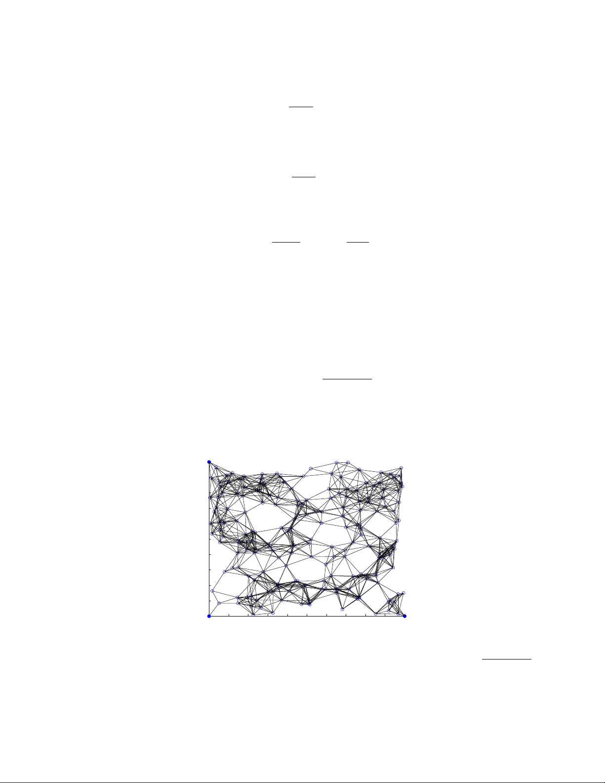
1 Rob ust Localization from Incomplete Local Information Amin Karbasi, Student Member , IEEE , Se woong Oh, Member , IEEE Abstract W e consider the problem of localizing wireless devices in an ad-hoc network embedded in a d - dimensional Euclidean space. Obtaining a good estimation of where wireless devices are located is crucial in wireless network applications including en vironment monitoring, geographic routing and topology control. When the positions of the devices are unknown and only local distance information is gi ven, we need to infer the positions from these local distance measurements. This problem is particularly challenging when we only hav e access to measurements that hav e limited accuracy and are incomplete. W e consider the extreme case of this limitation on the available information, namely only the connectivity information is av ailable, i.e., we only know whether a pair of nodes is within a fixed detection range of each other or not, and no information is known about ho w far apart they are. Further , to account for detection failures, we assume that even if a pair of devices is within the detection range, it fails to detect the presence of one another with some probability and this probability of failure depends on how far apart those devices are. Given this limited information, we in vestigate the performance of a centralized positioning algorithm M D S - M A P introduced by Shang et al. [SRZF03], and a distributed positioning algorithm H O P - T E R R A I N introduced by Sav arese et al. [SLR02]. In particular , for a network consisting of n devices positioned randomly , we provide a bound on the resulting error for both algorithms. W e show that the error is bounded, decreasing at a rate that is proportional to R Critical /R , where R Critical is the critical detection range when the resulting random network starts to be connected, and R is the detection range of each device. Amin Karbasi is with the School of Computer and Communication Sciences, Ecole Polytechnique F ´ ed ´ erale de Lausanne (EPFL), CH-1015 Lausanne, Switzerland (email: amin.karbasi@epfl.ch). Se woong Oh is with the department of Electrical En- gineering and Computer Science, Massachusetts Institute of T echnology (MIT), Cambridge, MA 02139 (email: swoh@mit.edu). A preliminary summary of this work appeared in [OKM10], [KO10]. July 16, 2021 DRAFT 2 I . I N T R O D U C T I O N In this paper, we address the problem of positoining (also referred to as sensor localization) when only a set of incomplete pairwise distances is provided. Location estimation of individual nodes is a requirement of many wireless sensor networks such as en vironment monitoring, geographic routing and topology control, to name only a few (for a thorough list of applications we refer the interested readers to [JH01], [Xu02]). In en vironment monitoring for instance, the measurement data by the wireless sensor network is essentially meaningless without knowing from where the data is collected. One way to acquire the positions is to equip all the sensors with a global positioning system (GPS). The use of GPS not only adds considerable cost to the system, but more importantly , it does not work in indoor environments or when the receiv ed GPS signal is jammed (see [CHH02] and the references therein for more information on this issue). As an alternativ e, we seek an algorithm that can deri ve positions of sensors based on local/basic information such as proximity (which nodes are within communication range of each other) or local distances (pairwise distances between neighbouring sensors). T wo common techniques for obtaining the local distance and connectivity information are Recei ved Signal Strength Indicator (RSSI) and Time Dif ference of Arri val (TDoA). RSSI is a measurement of the ratio of the power present in a recei ved radio signal and a reference po wer . Signal power at the receiving end is in versely proportional to the square of the distance between the receiv er and the transmitter . Hence, RSSI has the potential to be used to estimate the distance and it is common to assume the use of RSSI in distance measurements. Howe ver , experimental results indicate that the accuracy of RSSI is limited [PCB00]. TDoA technique uses the time difference between the receipt of two different signals with dif ferent velocities, for instance ultrasound and radio frequency signals [SHS01]. The time difference is proportional to the distance between the receiv er and the transmitter; and giv en the velocity of the signals, the distance can be estimated from the time difference. These techniques can be used, independently or together , for distance estimation. In an alternati ve approach, Angle of Arriv al (AoA) can also be used to infer the positions of sensors [NN01]. Once a node has the angle of arri val information from three other nodes with kno wn positions, we can perform triangulation to locate the wireless node. T o measure the angle of arri val, an antenna array is required at each wireless node. Gi ven a set of measurements, the problem of localization is solvable, meaning that it has a unique set of coordinates satisfying the gi ven local information, only if there are enough constraints. The simplest of such algorithms, i.e., multi dimensional scaling (MDS) [BG05], assumes that all pairwise distances are kno wn. Intuitiv ely , it is clear that with O ( n 2 ) pairwise distances we should be able to determine July 16, 2021 DRAFT 3 O ( n ) coordinates. Howe ver , in almost all practical scenarios such information is unav ailable for two major reasons. First, sensors are typically highly resource-constrained (e.g., power) and hav e limited communication range. Thus, far away sensors cannot communicate and obtain their pairwise distances. Second, due to noise and interference among sensors, there is always the possibility of non-detection or completely incoherent measurements. Many algorithms hav e been proposed to resolve these issues by using heuristic approximations to the missing distances, and their success has mostly been measured experimentally . Regarding the mechanisms deployed for estimating sensor locations, one can divide the localization algorithms into two categories: range-based and range-free. In the range-based protocols the absolute point-to-point distance estimates are used for inferring the locations, whereas in the range-free protocols no assumptions about the av ailability of such information are made and only the connectivity information is pro vided. As a result, range-free algorithms are more effecti ve in terms of stability and cost, hence more fav ourable to be deployed in practical settings. The theoretical guarantees associated with the performance of the existing methods are, howe ver , of the same interest and complementary in nature. Such analytical bounds on the performance of localization algorithms can provide answers to practical questions: for example, ” How large should the radio range be in order to get the reconstruction error within a threshold?” W ith this motiv ation in mind, our work takes a step forward in this direction. W e first focus on providing a bound on the performance of a popular localization algorithm M D S - M A P [SRZF03] when applied to sensor localization from only connectivity information. W e should stress here that pairwise distances are in variant under rigid transformations (rotation, translation and reflection). Hence, giv en connectivity information, we can only hope to determine the configuration or the relativ e map of the sensors. In other words, localization is possible only up to rigid transformations. W ith this point in mind, we prove that using M D S - M A P , we are able to localize sensors up to a bounded error in a connected network where most of pairwise distances are missing and only local connectivity information is gi ven. More precisely , assume that the network consists of n sensors positioned randomly in a d -dimensional unit cube with the radio range R = o (1) and detection probability p . Let the n × d matrices X and ˆ X denote the true sensor positions and their estimates by M D S - M A P , respectiv ely . Define L = I n × n − (1 /n ) 1 n 1 T n where I n × n is the identity matrix and 1 n is the all ones vector . It is not difficult to show that LX X T L satisfies nice properties, specifically , it is in variant under rigid transformations and if LX X T L = L ˆ X ˆ X T L , then X and ˆ X are equal up to rigid transformations. Therefore, we can naturally July 16, 2021 DRAFT 4 define the distance between X and ˆ X as follows: d inv ( X , b X ) = 1 n   LX X T L − L b X b X T L   F , where k · k F denote the Frobenius norm. Our first result establishes a bound on the error of M D S - M A P in terms of d inv , specifically , d inv ( X , b X ) ≤ R MDS R + o (1) , where R MDS = C d (ln( n ) /n ) 1 /d for some constant C d that only depends on the dimension d . One consequence of the ad-hoc nature of the underlying networks is the lack of a central infrastructure. This f act pre vents the use of common centralized positioning algorithms such as M D S - M A P . In particular , centralized algorithms suf fer from the scalability problem, and generally it is not feasible for them to be implemented in large scale sensor networks. Other disadvantages of centralized algorithms, as compared to distributed algorithms, are their requirements for higher computational complexity and lo wer reliability; these drawbacks are due to accumulated information inaccuracies caused by multi-hop transmission over a wireless network [MF A07]. W e then in vestigate an important question about whether similar performance guarantees can be obtained in a distributed setting where each sensor tries to estimate its own global position. As men- tioned above, this task cannot be accomplished unless some additional information, rather than local measurements, is provided. It is well known that in a d -dimensional Euclidean space, we need to know the global positions of at least d + 1 sensors, referred to as anc hors , in order to uniquely determine the global positions of the remaining sensors [NN01]. For the decentralized scenario, we turn our attention to analysing the performance of a popular localization algorithm called H O P - T E R R A I N algorithm [SLR02]. This algorithm can be seen as a distributed version of the M D S - M A P . Similar to M D S - M A P, we prov e that by using H O P - T E R R A I N , we are able to localize sensors up to a bounded error in a connected network where most of the pairwise distances are unkno wn and only local connectivity information is giv en. More formally , assume that the network consists of n sensors positioned randomly in a d -dimensional unit cube and d + 1 anchors in general positions. Moreov er , we let the radio range R = o (1) and denote the detection probability by p . W e sho w that when only connectivity information is a vailable, for ev ery unkno wn node i , the Euclidean distance between the estimate ˆ x i and the correct position x i is bounded by k x i − ˆ x i k ≤ R HOP R + o (1) , where R HOP = C 0 d (log n/n ) 1 d for some constant C 0 d that only depends on d . July 16, 2021 DRAFT 5 T ABLE I D I S T R I B U T E D L O C A L I Z A T I O N A L G O R I T H M C L A S S I FI C A T I O N [ L R 0 3 ] Phase Robust positioning Ad-hoc positioning N -hop multilateration 1. Distance DV - H O P Euclidean Sum-dist 2. Position Lateration Lateration Min-max 3. Refinement Y es No Y es I I . R E L AT E D W O R K The localization problem and its v ariants has attracted significant research interest in recent years. A general surv ey of the area and an overvie w of recent techniques can be found in [NN01] and [MF A07], respecti vely . The problem is also closely related to dimensionality reduction [RS00] and manifold learning [SR03] in which the objects/data come from a high dimensional space, and the goal is to compute a lo w-dimensional, neighbourhood preserving embeddings. In the case when all pairwise distances are known, the coordinates can be deriv ed by using a classical method known as multidimensional scaling (MDS) [BG05]. The underlying principle of the MDS is to con vert distances into an inner product matrix, whose eigen vectors are the unknown coordinates. In the presence of noise, MDS tolerates errors gracefully due to the ov erdetermined nature of the solution. Ho wever , when most pairwise distances are missing, the problem of finding the unkno wn coordinates becomes more challenging. For centralized algorithms (where all the measurements are sent to a single processor and the estimated positions are computed) three types of practical solutions to the abo ve problem hav e been proposed in the literature. The first group consists of algorithms that try first to estimate the missing entries of the distance matrix and then apply MDS to the reconstructed distance matrix to find the coordinates of the sensors. M D S - M A P , introduced in [SRZF03] and further studied in [SRZF04], can be mentioned as a well-known example of this class where it computes the shortest paths between all pairs of nodes in order to approximate the missing entries of the distance matrix. The algorithms in the second group mainly consider the sensor localization as a non-con vex optimization problem and directly estimate the coordinates of sensors. A famous example of this type is a relaxation to semidefinite programming (SDP)[BY04]. In the third group, the problem is formulated through a stochastic optimization where the main technique used in these algorithms is the stimulated annealing, which is a generalization of the Monte Carlo method in combinatorial optimization [KMV06], [KM06]. July 16, 2021 DRAFT 6 Perhaps a more practical and interesting case is when there is no central infrastructure. [LR03] identifies a common three-phase structure of three, popular , distrib uted sensor -localization algorithms, namely robust positioning [SLR02], ad-hoc positioning [NN03] and N-hop multilateration [SPS03]. T able I illustrates the structure of these algorithms. In the first phase, nodes share information to collectiv ely determine the distances from each of the nodes to a number of anchors. Anchors are special nodes with a priori kno wledge of their o wn position in some global coordinate system. In the second phase, nodes determine their position based on the estimated distances to the anchors provided by the first phase and the known positions of the anchors. In the last phase, the initial estimated positions are iterativ ely refined. It is empirically demonstrated that these simple three-phase distributed sensor-localization algorithms are robust and ener gy-efficient [LR03]. Howe ver , depending on which method is used in each phase, there are different tradeof fs between localization accuracy , computation complexity and po wer requirements. In [NSB03], a distributed algorithm-called the Gradient algorithm- was proposed; it is similar to ad-hoc positioning [NN03] b ut uses a different method for estimating the av erage distance per hop. Another distributed approach introduced in [IFMW04] is to pose the localization problem as an inference problem on a graphical model and solve it by using Nonparametric Belief Propagation (NBP). It is naturally a distributed procedure and produces both an estimate of sensor locations and a representation of the location uncertainties. The estimated uncertainty may subsequently be used to determine the reliability of each sensor’ s location estimate. The performances of these practical algorithms are in variably measured through simulations and little is kno wn about the theoretical analysis supporting their results. A fe w exceptions are in the following work. In [DJMI + 06] the authors use matrix completion methods [Faz02] as a means to reconstruct the distance matrix. The main contribution of their paper is that they are able to provably localize the sensors up to a bounded error . Howe ver , their analysis is based on a number of strong assumptions. First, they assume that ev en far -away sensors ha ve a non-zero probability of detecting their distances. Second, the algorithm explicitly requires the kno wledge of detection probabilities between all pairs. Third, their theorem only works when the av erage degree of the network (i.e., the average number of nodes detected by each sensor) gro ws linearly with the number of sensors in the network. Our first result, specifically the analysis of M D S - M A P , has a similar flav our as in[DJMI + 06]. W e provide a theoretical guarantee that backs up experimental results. W e use shortest paths as our primary guess for the missing entries in the distance matrix and apply MDS to find the topology of the network. In contrast to [DJMI + 06], we require weaker assumptions for our results. More specifically , we assume that only neighbouring sensors hav e information about each other and that only connecti vity information July 16, 2021 DRAFT 7 is known. Furthermore, the knowledge of detection probabilities plays no role in our analysis or the algorithm. And last, in our analysis we assume that the average degree grows logarithmically-not linearly- with the number of sensors, which results in needing many less rev ealed entries in the distance matrix. In particular, the last condition is quite realistic: If the a verage degree grows any slower then the network is not even connected (more on this issue in Section IV -C). As the shortest paths algorithm works for both rage-free and range-aware cases, our analysis includes both and provides the first error bounds on the performance of M D S - M A P . Of particular interest are the two ne w results on the performance of sensor localization algorithms. In [JM11], Jav anmard et al. proposes a new reconstruction algorithm based on semidefinite programming where they could establish lower and upper bounds on the reconstruction errors of their algorithm. Similarly , in [KOPV10], due to ne w adv ances in matrix completion methods [CR08], the authors analyse the performance of OptSpace [KM10], a novel matrix completion algorithm, in localizing the sensors. Interestingly , they did not need to adhere to the assumptions made by [DJMI + 06]. Howe ver , they hav e a restricti ve assumption about the topology of the network, specifically , sensors are scattered inside an annulus. All the abov e analytical results crucially rely on the fact that there is a central processor with access to the inter-sensor distance measurements. Howe ver , as we hav e mentioned earlier, centralized algorithms suf fer from the scalability problem and require higher computational complexity . Hence, a distributed algorithm with similar a performance bound is desirable. In our second result, we analyse the recon- struction error of a distributed sensor localization algorithm. T o the best of our knowledge we sho w for the first time that H O P - T E R R A I N , introduced in [SLR02], achiev es a bounded error when only local connecti vity information is giv en. Finally , one of the fundamental challenges in localization problem is whether, giv en a set of mea- surements, the sensor network is uniquely localizable or not. In the noiseless setting where all the measurements are accurate, it was shown that the correct notion through which we can answer this question is the global rigidity [MWY06], a property that is easy to check (a thorough discussion of global rigidity and its implications for the sensor localization problem is gi ven in [GHDT10]). Ho wev er , finding such a unique solution is NP-hard [JJ05]. In the case of noisy distance measurements v ery little is kno wn in this area. For instance, we do not know the fundamental limits for sensor localization algorithms or whether there are any algorithms with prov en guarantees. From this point of view , our results narrow the gap between the algorithmic aspect of sensor localization and the theoretical one. In particular , we sho w that ev en in the presence of noise, the M D S - M A P and H O P - T E R R A I N algorithms can localize July 16, 2021 DRAFT 8 the nodes within a bounded error . The organization of this paper is as follows. In Section III we introduce the model and the notation used in our work. In Section IV we describe the M D S - M A P and H O P - T E R R A I N algorithms and their common features. Our results are stated in Section V where we provide their proofs in Section VI. Finally , we conclude in Section VII. I I I . M O D E L D E FI N I T I O N Before discussing the centralized and distrib uted localization algorithms in detail, we define the math- ematical model considered in this work. First, we assume that we hav e no fine control ov er the placement of the sensors that we call the unknown nodes (e.g., the nodes are dropped from an airplane). F ormally , we assume that n nodes are placed uniformly at random in a d -dimensional cube [0 , 1] d . Additionally , we assume that there are m special sensors, which we call anchors , with a priori kno wledge of their own positions in some global coordinate. In practice, it is reasonable to assume that we hav e some control ov er the position of anchors. Basically , anchors are the nodes that are planted on the field before an y positioning takes place. Let V a = { 1 , . . . , m } denote the set of m vertices corresponding to the anchors and V u = { m + 1 , . . . , m + n } the set of n vertices corresponding to the unknown nodes. W e use x i to denote the random position of the node i and X to denote the n × d position matrix where the i -th row corresponds to x i . In positioning applications, due to attenuation and power constraints, only measurements between close-by nodes are av ailable. As a result, the pairwise distance measurements can be represented by a random geometric graph G ( n + m, R ) = ( V , E , P ) , where V = V u ∪ V a , E ⊆ V × V is a set of undirected edges that connect pairs of sensors that are close to each other, and P : E → R + is a non-negati ve real-v alued function. The function P is a mapping from a pair of connected nodes ( i, j ) ∈ E to a distance measurement between i and j . A common model for this random geometric graph is the disc model where node i and j are connected if the Euclidean distance d i,j ≡ k x i − x j k is less than or equal to a positi ve radio range R . In formulae, ( i, j ) ∈ E ⇔ d i,j ≤ R . As mentioned earlier , there are a variety of ways to measure the connectivity between two nodes, including time difference of arriv al and RF receiv ed-signal strength (also called RF ranging). Due to limited resources, in all of the mentioned solutions there is a probability of non-detection (or completely wrong estimation). Think of RF ranging in the presence of an obstacle or in the (frequent) case of multiple July 16, 2021 DRAFT 9 x p ( z ) y Fig. 1. This plot shows how the probability of detection changes as the distance between two sensor changes. paths. Depending on the acquisition mechanism, this may result in the absence of measurement or in incoherent measurements. Throughout this paper , to model this failure of detection, we assume that two nodes can detect each other with a probability that only depends on the distance d i,j . Namely , ( i, j ) ∈ E with probability p ( d i,j ) if d i,j ≤ R . The detection probability p ( · ) : [0 , R ] → [0 , 1] is a non-increasing function of the distance. W e consider a simple function parameterized by two scalar v alues α ∈ (0 , 1] and β ∈ [0 , 3) : p ( z ) = min  1 , α  z R  − β  , (1) for α ∈ (0 , 1] and β ∈ [0 , d ) . Note that this includes the disc model with perfect detection as a special case (i.e., α = 1 , β = 0 ). T o each edge ( i, j ) ∈ E , we associate the distance measurement P i,j between sensors i and j . In an ideal case, we hav e exact distance measurements av ailable for those pairs in E . This is called the rang e-based model or the range-aware model. In formulae, P i,j =    d i,j if ( i, j ) ∈ E , ∗ otherwise , where a ∗ denotes that the distance measurement is unav ailable. In this paper , we assume that we are giv en only network connectivity information and no distance July 16, 2021 DRAFT 10 Connected Disconnected a b c R Fig. 2. This example shows the model we consider in this work. Nodes a and b are connected since they are within radio range R from each other . Even though the similar situation presents for b and c , they are not connected due to detection failure. Finally , nodes a and c are not connected because they are far apart. information. This is kno wn as the connectivity-based model or the range-free model. More formally , P i,j =    1 if ( i, j ) ∈ E , ∗ otherwise . In the follo wing, let D denote the n × n squared distance matrix where D i,j = d 2 i,j . By definition, D = a 1 T n + 1 n a T − 2 X X T , where a ∈ R n is a vector with a i = k x i k 2 and 1 n is the all ones vector . As D is a sum of two rank-1 matrices and a rank- d matrix, its rank is at most d + 2 . I V . A L G O R I T H M S In general, there are two solutions to the localization problem: a relativ e map and an absolute map. A relati ve map is a configuration of sensors that ha ve the same neighbor relationships as the underlying graph G . In the following we use the terms configuration, embedding, and relativ e map interchangeably . An absolute map, on the other hand, determines the absolute geographic coordinates of all sensors. In this paper our objectiv e is two-fold. First, we present the centralized algorithm M D S - M A P , that finds a configuration that best fits the proximity measurements. Then, we discuss its distributed version H O P - T E R R A I N where its goal is for each sensor to find its absolute position. For both, we provide analytical bounds on the error between the estimated configuration and the correct configuration. July 16, 2021 DRAFT 11 T ABLE II S U M M A RY O F N OTA T I O N . n number of unknown sensors V u set of unknown nodes m number of anchors V a set of anchors R communication range 1 n all ones vector of size n P i,j distance measurements b D estimated squared distance matrix d i,j Pairwise distance between nodes i and j I n × n n × n identity matrix x i position of node i ˆ x i estimated position of node i p detection probability X positions matrix d dimension b X estimated positions matrix D squared distance matrix ˆ d i,j shortest path between node i and j O ( d ) orthogonal group of d × d matrices k · k F Frobenius norm h A, B i Frobenius inner product k · k 2 spectral norm A. Centralized P ositioning Algorithm: M D S - M A P For the centralized positioning algorithm, we assume that there is no anchor node in the system, namely , V a = φ . W e define a set of random positions of n sensors X = { x 1 , . . . , x n } . M D S - M A P consists of two steps: Algorithm : M D S - M A P [SRZF03] Input: dimension d , graph G = ( V , E , P ) 1: Compute the shortest paths, and let b D be the squared shortest paths matrix; 2: Apply MDS to b D , and let b X be the output. Shortest paths. The shortest path between nodes i and j in graph G = ( V , E , P ) is defined as a path between two nodes such that the sum of the proximity measures of its constituent edges is minimized. Let ˆ d i,j be the computed shortest path between node i and j . Then, the squared shortest paths matrix b D ∈ R n × n is defined as b D ij = ˆ d 2 i,j for i 6 = j , and 0 for i = j . Multidimensional scaling. In step 2, we apply the MDS to b D to get a good estimate of X , specifically , we compute b X = MDS d ( b D ) . Multidimensional scaling (MDS) refers to a set of statistical techniques used in finding the configuration of objects in a low dimensional space such that the measured pairwise distances are preserved [BG05]. It is often used for a visual representation of the proximities between a set of items. For e xample, gi ven a matrix of percei ved similarities or dissimilarities between n items, MDS geometrically places each of those items in a low dimensional space such that the items that are similar are placed close to each other . Formally , MDS finds a lower dimensional embedding ˆ x i s that July 16, 2021 DRAFT 12 i a 1 a 2 a 3 3 R 2 R 2 R Fig. 3. The shortest path between two nodes is defined in terms of the minimum number of hops multiplied by the radio range R . For instance, the shortest path between i and a 1 is 2 R . minimize the str ess defined as stress . = v u u t P i 6 = j ( f ( d i,j ) − ˆ d i,j ) 2 P i 6 = j ˆ d 2 i,j , where d i,j is the input similarity (or dissimilarity), ˆ d i,j = k ˆ x i − ˆ x j k is the Euclidean distance in the lower dimensional embedding, and f ( · ) is some function on the input data. When MDS perfectly embeds the input data, we will ha ve f ( d i,j ) = ˆ d i,j and the stress is zero. In this chapter we use what is called the classic metric MDS (we refer the interested reader to [CC01], for the definition of other types of MDS algorithms, for instance non-metric MDS, replicated MDS, and weighted MDS). In classic metric MDS, f ( · ) is the identity function and the input dissimilarities correspond to the Euclidean distances such that d i,j = k x i − x j k for some lo wer dimensional embedding { x i } . Further , when all the dissimilarities (or pairwise distances) are measured without error, the follo wing spectral method correctly reco vers the lo wer dimensional embedding up to a rigid motion. July 16, 2021 DRAFT 13 Algorithm : Classic Metric MDS [SRZF03] Input: dimension d , estimated distance matrix M 1: Compute ( − 1 / 2) LM L , where L = I n − (1 /n ) 1 n 1 T n ; 2: Compute the best rank- d approximation U d Σ d U T d of ( − 1 / 2) LM L ; 3: Return MDS d ( M ) ≡ U d Σ 1 / 2 d . This algorithm has been frequently used in positioning applications; and in the future, whene ver we say MDS we refer to the abo ve algorithm. Let L be an n × n symmetric matrix such that L = I n − (1 /n ) 1 n 1 T n , where 1 n ∈ R n is the all ones vector and I n is the n × n identity matrix. Let MDS d ( D ) denote the n × d matrix returned by MDS when applied to the squared distance matrix D . Then, in formula, gi ven the singular value decomposition (SVD) of a symmetric and positive definite matrix ( − 1 / 2) LD L as ( − 1 / 2) LD L = U Σ U T , MDS d ( D ) ≡ U d Σ 1 / 2 d , where U d denotes the n × d left singular matrix that corresponds to the d lar gest singular values and Σ d denotes the d × d diagonal matrix with d largest singular v alues in the diagonal. This is also known as the M D S L O C A L I Z E algorithm in [DJMI + 06]. Note that as the columns of U are orthogonal to 1 n by construction, it follo w that L · MDS d ( D ) = MDS d ( D ) . It can be easily shown that when MDS is applied to the correct squared distance matrix without noise, the configuration of sensors are exactly recovered [DJMI + 06]. This follows from the following equality − (1 / 2) LD L = LX X T L . (2) Note that we only obtain the configuration and not the absolute positions, in the sense that MDS d ( D ) is one v ersion of infinitely man y solutions that matches the distance measurements D . Therefore there are multiple incidents of X that result in the same D . W e introduce a formal definition of rigid transformation and related terms. W e denote by O ( d ) the orthogonal group of d × d matrices. A set of sensor positions Y ∈ R n × d is a rigid transformation of X , if there exists a d -dimensional shift vector s and an orthogonal matrix Q ∈ O ( d ) such that Y = X Q + 1 n s T . Here Y should be interpreted as a result of first rotating (and/or July 16, 2021 DRAFT 14 reflecting) sensors in position X by Q and then adding a shift by s . Similarly , when we say two position matrices X and Y are equal up to a rigid transformation, we mean that there exists a rotation Q and a shift s such that Y = X Q + 1 n s T . Also, we say a function f ( X ) is invariant under rigid transformation if and only if for all X and Y that are equal up to a rigid transformation we have f ( X ) = f ( Y ) . Under these definitions, it is clear that D is in variant under rigid transformation, as for all ( i, j ) , D ij = k x i − x j k 2 = k ( x i Q + s T ) − ( x j Q + s T ) k 2 , for any Q ∈ O ( d ) and s ∈ R d . Although MDS works perfectly when D is av ailable, in practice not all proximity measurements are av ailable because of the limited radio range R . This is why , in the first step, we estimated the unav ailable entries of D by finding the shortest path between disconnected nodes. B. Distributed P ositioning Algorithm: H O P - T E R R A I N Recall that H O P - T E R R A I N is a distrib uted algorithm that aims at finding the global map. Notice that in order to fix the global coordinate system in a d dimensional space, we need to know the positions of at least d + 1 nodes. As we defined before, these nodes whose global positions are kno wn are called anchors. In this section we assume that we have m anchors in total, i.e., V a = { 1 , 2 , . . . , m } . Based on the robust positioning algorithm introduced in [SLR02], the distributed sensor localization algorithm consists of two steps : Algorithm : H O P - T E R R A I N [SLR02] 1: Each node i computes the shortest paths { ˆ d i,a : a ∈ V a } between itself and the anchors; 2: Each node i deriv es an estimated position ˆ x i by triangulation with a least squares method. Distributed shortest paths: Similarly to M D S - M A P , the first step is about finding the shortest path. The difference is that in the first step each of the unknown nodes only estimates the distances between itself and the anchors. These approximate distances will be used in the ne xt triangulation step to deriv e an estimated position. In other w ords, the shortest path between an unkno wn node i and an anchor a in the graph G pro vides an estimate for the Euclidean distance d i,a = k x i − x a k . W e denote by ˆ d i,a the computed shortest path and this provides the initial estimate for the distance between the node i and the anchor a . When only the connectivity information is av ailable and the corresponding graph G = ( V , E , P ) is defined as in the connectivity-based model , the shortest path ˆ d i,a July 16, 2021 DRAFT 15 is equiv alent to the minimum number of hops between a node i and an anchor a multiplied by the radio range R . In order to find the minimum number of hops from an unknown node i ∈ V u to an anchors a ∈ V a in a distributed way , we use a method similar to DV - H O P [NN03]. Each unkno wn node maintains a table { x a , h a } that is initially empty , where x a ∈ R d refers to the position of the anchor a and h a to the number of hops from the unknown node to the anchor a . First, each of the anchors initiate a broadcast containing its known location and a hop count of one. All of the one-hop neighbors surrounding the anchor , on recei ving this broadcast, record the anchor’ s position and a hop count of one, and then broadcast the anchor’ s known position and a hop count of two. From then on, whenever a node recei ves a broadcast, it does one of the tw o things. If the broadcast refers to an anchor that is already in the record and the hop count is larger than or equal to what is recorded, then the node does nothing. Otherwise, if the broadcast refers to an anchor that is ne w or has a hop count that is smaller , the node updates its table with this ne w information on its memory and broadcasts the new information after incrementing the hop count by one. T o estimate the distances between the node and the anchors, when ev ery node has computed the hop count to all the anchors, the number of hops is multiplied by the radio range R to estimate the distances between the node and the anchors. Note that to begin triangulation, not all the hop counts to all the anchors are necessary . A node can start triangulation as soon as it has estimated distances to d + 1 anchors. There is an ob vious trade-off between the number of communications and their performance. The abo ve step of computing the minimum number of hops is the same distrib uted algorithm as described in D V - H O P . Howe ver , one dif ference is that instead of multiplying the number of hops by a fixed radio range R , in D V - H O P , the number of hops is multiplied by an average hop distance. The av erage hop distance is computed from the known pairwise distances between anchors and the number of hops between the anchors. although numerical simulations show that the a verage hop distance provides a better estimate, the difference between the computed av erage hop distance and the radio range R becomes negligible as n grows lar ge. T riangulation using least squares. In the second step, each unknown node i ∈ V u uses a set of estimated distances { ˆ d i,a : a ∈ V a } together with the known positions of the anchors, to perform a triangulation. The resulting estimated position is denoted by ˆ x i . For each node, the triangulation consists in solving a single instance of a least squares problem ( Ax = b ) and this process is kno wn as Lateration [SRB01], [LR03]. July 16, 2021 DRAFT 16 x 1 x 2 x 3 x 1 x 2 x 3 Fig. 4. Multilateration with exact distance measurements (left) and with approximate distance measurements (right). Three solid circles denote the anchors (red) and the white circle denotes the unknown nodes. The intersection of the blue lines corresponds to the solution of multilateration. For an unknown node i , the position vector x i and the anchor positions { x a : a ∈ { 1 , . . . , m }} satisfy the follo wing series of equations: k x 1 − x i k 2 = d 2 i, 1 , . . . k x m − x i k 2 = d 2 i,m . Geometrically , the abov e equalities simply say that the point x i is the intersection point of m circles centred at x 1 , x 2 , . . . , x m (see Figure 4). This set of equations can be linearised by subtracting each line from the next line. k x 2 k 2 − k x 1 k 2 + 2( x 1 − x 2 ) T x i = d 2 i, 2 − d 2 i, 1 , . . . k x m k 2 − k x m − 1 k 2 + 2( x m − 1 − x m ) T x i = d 2 i,m − d 2 i,m − 1 . July 16, 2021 DRAFT 17 By reordering the terms, we get a series of linear equations for node i in the form A x i = b ( i ) 0 , for A ∈ R ( m − 1) × d and b ∈ R m − 1 defined as A ≡      2( x 1 − x 2 ) T . . . 2( x m − 1 − x m ) T      , b ( i ) 0 ≡      k x 1 k 2 − k x 2 k 2 + d 2 i, 2 − d 2 i, 1 . . . k x m − 1 k 2 − k x m k 2 + d 2 i,m − d 2 i,m − 1      . Note that the matrix A does not depend on the particular unknown node i and all the entries are kno wn accurately to all the nodes after the distributed shortest paths step. Howe ver , the vector b ( i ) 0 is not av ailable at node i , because d i,a ’ s are not known. Hence we use an estimation b ( i ) , that is defined from b ( i ) 0 by replacing d i,a by ˆ d i,a e verywhere. Notice that ˆ d i,a ≥ d i,a . As a result, the circles centred at x 1 , x 2 , . . . , x m hav e potentially larger radii. Therefore, the intersection between circles is no longer a single point, but rather a closed area. Then, finding the optimal estimation ˆ x i of x i that minimizes the mean squared error is solved in a closed form using a standard least squares approach: ˆ x i = ( A T A ) − 1 A T b ( i ) . (3) For bounded d = o (1) , a single least squares operation has comple xity O ( m ) , and applying it n times results in the ov erall complexity of O ( n m ) . No communication between the nodes is necessary for this step. C. Str etch F actor: Euclidean Distance versus Shortest P ath In general when the graph G is not connected, the localization problem is not well defined. In fact, there are multiple configurations resulting in the same observed proximity measures. For instance if graph G consists of two disconnected components, the y can be placed in possibly infinitely different ways with respect to each other without violating any constraints imposed by G . For this reason we restrict our attention to the case where G is connected. In this work, we are interested in a scalable system of n unkno wn nodes for a large v alue of n . As n gro ws, it is reasonable to assume that the average number of connected neighbours for each node should stay constant. This happens, in our model, if we chose the radio range R = C /n 1 /d . Howe ver , in the unit square, assuming sensor positions are drawn uniformly , the random geometric graph is connected, with July 16, 2021 DRAFT 18 Fig. 5. The red vertices indicate the anchors. Under the right scaling of the radio range R , the graph stays connected (left figure) whereas otherwise there will be nodes without any means of communication to others (right graph). high probability , if π R 2 > (log n + c n ) /n for c n → ∞ [GK98]. A similar condition can be derived for generic d -dimensions as C d R d > (log n + c n ) /n , where C d ≤ π is a constant that depends on d . Moreov er , in case C d R d < (log n + c n ) /n , not only the graph is not connected, there will be isolated nodes with hight probability . Since isolated nodes cannot communicate with other sensors, there is no way to find their shortest paths to other nodes. Consequently , both M D S - M A P and H O P - T E R R A I N algorithms will be in trouble (see Figure 5). Hence, instead of R = C /n 1 /d , we focus in the regime where the av erage number of connected neighbors is slowly increasing with n . Let R critical be the critical detection range where the resulting graph starts to be connected. Then we are interested in the regime R = C R Critical , for some positi ve constant C ≥ 1 such that the graph stays connected with high probability . In our analysis, the key observation and the crux of the argument is to show that the shortest-path estimate is guaranteed to be arbitrarily close to the correct distance for large enough radio range R and large enough n . Once we pro ved this, we can then show that the MDS step (equi valently , lateration) finds almost correctly the relati ve (equiv alently , global) position of the sensors. W e demonstrate ho w the error in estimating the Euclidean distance will be reflected on the position estimation. The precise statements are gi ven in Section V. W e have already discussed the complexity of MDS and lateration steps. T o complete our discussion we need to e valuate the complexity of finding the shortest path. In the M D S - M A P algorithm we require that all-pairs shortest paths be found. This problem has an efficient algorithm whose complexity is July 16, 2021 DRAFT 19 O ( n 2 log n + n | E | ) [Joh77]. For R = C (log n/n ) 1 /d with constant C , the graph is sparse with | E | = O ( n log n ) , whence the complexity is O ( n 2 log n ) . Contrary to M D S - M A P , in H O P - T E R R A I N we must only compute the shortest paths between the unknown nodes and the anchors. This distributed shortest paths algorithm can be done ef ficiently with total complexity of O ( n m ) . V . M A I N R E S U LT S In this section we present our main results regarding the performance of M D S - M A P and H O P - T E R R A I N algorithms. A. M D S - M A P Our first result establishes an upper bound on the error achiev ed by M D S - M A P when we have only the connecti vity information as in the case of the connectivity-based model . Let b X denote an n × d estimation for X with an estimated position for node i in the i th row . Then, we need to define a metric for the distance between the original position matrix X and the estimation b X , which is in v ariant under rigid transformation of X or b X . Define L ≡ I n − (1 /n ) 1 n 1 T n as in the MDS algorithm. L is an n × n rank n − 1 symmetric matrix, which eliminates the contrib utions of the translation, in the sense that LX = L ( X + 1 s T ) for all s ∈ R d . Note that L has the follo wing nice properties: 1) LX X T L is in variant under rigid transformation. 2) LX X T L = L b X b X T L implies that X and b X are equal up to a rigid transformation. This naturally defines the follo wing distance between X and b X . d inv ( X , b X ) = 1 n   LX X T L − L b X b X T L   F , (4) where k A k F = ( P i,j A 2 ij ) 1 / 2 denotes the Frobenius norm. Notice that the factor (1 /n ) corresponds to the usual normalization by the number of entries in the summation. Indeed this distance is in variant to rigid transformation of X and b X . Furthermore, d inv ( X , b X ) = 0 implies that X and b X are equal up to a rigid transformation. W ith this metric, our main result establishes an upper bound on the resulting error . The proof of this theorem is pro vided in Section VI. W e define R MDS ≡ 32  12 log n α ( n − 2)  1 d . (5) Theor em 5.1 (connectivity-based model): Assume n nodes are distrib uted uniformly at random in the [0 , 1] d hypercube, for a bounded dimension d ∈ { 2 , 3 } . For a positiv e radio range R and detection July 16, 2021 DRAFT 20 probability p defined in (1), we are gi ven the connectivity information of the nodes according to the range-free model with probabilistic detection. Then, with a probability larger than 1 − 1 /n 4 , the distance between the estimate b X produced by M D S - M A P and the correct position matrix X is bounded by d inv ( X , b X ) ≤ R MDS R + 20 R , (6) for R > (1 /α ) 1 /d R MDS , where d inv ( · ) is defined in (4) and R MDS in (5). The proof is provided in Section VI. The follo wing corollary trivially follows, as for each ( i, j ) ∈ E , we hav e d i,j ≤ R . Cor ollary 5.2 (rang e-based model): Under the hypotheses of Theorem 5.1 and in the case of rang- based model, with high probability d inv ( X , b X ) ≤ R MDS R + 20 R . As described in the previous section, we are interested in the regime where R = C (log n/n ) 1 /d for some constant C . Giv en a small positive constant δ , this implies that M D S - M A P is guaranteed to produce estimated positions that satisfy d inv ( X , b X ) ≤ δ with a large enough constant C and a lar ge enough n . When α is fixed and R = C (log n/n ) 1 /d for some positi ve parameter C , the error bound in (6) becomes d inv ( X , b X ) ≤ C 1 C α 1 /d + C 2 C  log n n  1 /d , for some numerical constants C 1 and C 2 . The first term is in versely proportional to C and α 1 /d and is independent of n , whereas the second term is linearly dependent on C and v anishes as n grows large. This is illustrated in Figure 6, which sho ws numerical simulations with n sensors randomly distributed in the 2-dimensional unit square. Notice that the resulting error is in versely proportional to α and independent of β . Remark 5.3: Even though the upper bounds for both range-free and range-based models have the same form, there is a slight difference between their behaviours as R gro ws. In the range-free case, up to some point, the performance of M D S - M A P improves as R increases. This is due to the fact that the first and second terms go in opposite directions as a function of R . Howe ver , In the range-based case, as R increases, we obtain a more accurate estimate of the the Euclidean distance. As a result, once the radio range increases, the resulting error of M D S - M A P decreases and we do not see the contribution of the second term. This phenomenon is illustrated in Figure 7. Using the above theorem, we can further show that there is a linear transformation S ∈ R d × d , such that when applied to the estimations, we get a similar bound in the Frobenius norm of the error in the positions. July 16, 2021 DRAFT 21 0.03 0.06 0.12 0 10 20 30 40 50 60 70 C A verage Error α = 0 . 25 , β = 1 α = 0 . 5 , β = 0 α = 0 . 5 , β = 1 α = 0 . 5 , β = 2 α = 1 , β = 1 Fig. 6. A verage distance between the correct topology X and the estimation ˆ X using M D S - M A P as a function of C where the radio range is R = C p log n/n . The n = 1 , 000 sensors are distributed randomly on a unit square under range-free model. V arious values of α and β are used where two nodes at distance r are detected with probability p ( r ) = min { 1 , α ( R/r ) β } . 0.0001 0.001 0.01 0 10 20 30 40 50 60 70 C A verage Error α = 0 . 25 , β = 1 α = 0 . 5 , β = 0 α = 0 . 5 , β = 1 α = 0 . 5 , β = 2 α = 1 , β = 1 Fig. 7. A verage error of M D S - M A P under the range-based model. Theor em 5.4: Under the hypotheses of Theorem 5.1, with high probability min S ∈ R d × d 1 √ n k LX − L b X S k ≤ √ 6  R MDS R + 20 R  Remark 5.5: Note that although for the sake of simplicity , we focus on [0 , 1] d hypercube; our analysis easily generalizes to any bounded con ve x set and homogeneous Poisson process model with density ρ = n . The homogeneous Poisson process model is characterized by the probability that there are exactly k nodes appearing in any region with volume A : P ( k A = k ) = ( ρA ) k k ! e − ρA . Here, k A is a random variable July 16, 2021 DRAFT 22 defined as the number of nodes in a region of volume A . Remark 5.6: T o simplify calculations, we assumed that d is either 2 or 3 . Ho wever , the analysis easily applies to general d and only the constant in the bound (6) would change as long as d = O (1) . In what follows we inv estigate an important question whether similar performance guarantees, as in M D S - M A P , can be obtained in a distributed setting. In particular , we analyze the performance of the H O P - T E R R A I N algorithm. As we have already stressed, this algorithm can be seen as a distributed version of the M D S - M A P algorithm. In particular, we show that when only connectivity information is av ailable, for every unknown node. The Euclidean distance between the estimate and the correct position can be bounded v ery similarly to Theorem 5.1. B. H O P - T E R R A I N Our second result establishes that H O P - T E R R A I N [SLR02] achie ves an arbitrarily small error for a radio range R = C (log n/n ) 1 /d with a large enough constant C , when we have only the connectivity information as in the case of the connectivity-based model . The same bound holds immediately for the range-based model , when we ha ve an approximate measurements for the distances, and the same algorithm can be applied without any modification. to compute better estimates for the actual distances between the unkno wn nodes and the anchors, the e xtra information can be readily incorporated into the algorithm. W e define R HOP ≡ 12  12 log n α ( n − 2)  1 d . (7) Theor em 5.7: Assume n sensors and m anchors are distributed uniformly at random in the [0 , 1] d hypercube for a bounded dimension d ∈ { 2 , 3 } . For a given radio range R > (1 /α ) 1 /d R HOP , detection probability p defined in (1), and the number of anchors m = Ω(log n ) , the follo wing is true with probability at least 1 − 1 /n 4 . For all unkno wn nodes i ∈ V u , the Euclidean distance between the estimate ˆ x i gi ven by H O P - T E R R A I N and the correct position x i is bounded by k x i − ˆ x i k ≤ R HOP R + 24 R . (8) The proof is provided in Section VI. As described in the previous section, we are interested in the regime where R = C (log n/n ) 1 /d for some constant C . Gi ven a small positi ve constant δ , this implies that H O P - T E R R A I N is guaranteed to produce estimated positions that satisfy k x i − ˆ x i k ≤ δ for all i ∈ V u with a lar ge enough constant α and large enough n . July 16, 2021 DRAFT 23 Anchors Unknown Nodes R Fig. 8. Three anchors in fixed positions ( [0 , 0] , [1 , 0] , [0 , 1] ) for a two-dimensional sensor localization. When the number of anchors is bounded and the positions of the anchors are chosen randomly , it is possible that, in the triangulation step, we get an ill-conditioned matrix A T A , resulting in an large estimation error . This happens, for instance, if three anchors fall close to a line. Howe ver , as mentioned in the introduction, it is reasonable to assume that, for the anchors, the system designer has some control ov er where they are placed. In that case, the next remark shows that when the positions of anchors are properly chosen, only d + 1 anchors suffice to get a similar bound on the performance. Note that this is the minimum number of anchors necessary for triangulation. For simplicity we assume that one anchor is placed at the origin and d anchors are placed at positions corresponding to d -dimensional unit vectors. The position of the d + 1 anchors are { [0 , . . . , 0] , [1 , 0 , . . . , 0] , [0 , 1 , 0 , . . . , 0] , [0 , . . . , 0 , 1] } . (see figure 8) Theor em 5.8: Assume that n sensors are distributed uniformly at random in the [0 , 1] d hypercube for a bounded dimension d = { 2 , 3 } . Also, assume that there are d + 1 anchors, one of which is placed at the origin, and the position vectors of the d remaining anchors are the d -dimensional unit vectors. For a given radio range R > (1 /α ) 1 /d R HOP and detection probability p defined in (1) the following is true with probability at least 1 − 1 /n 4 . For all unknown nodes i ∈ V u , the Euclidean distance between the estimate ˆ x i gi ven by H O P - T E R R A I N and the correct position x i is bounded by k x i − ˆ x i k ≤ 2 R HOP R + 48 R . (9) The proof is pro vided in Section VI. July 16, 2021 DRAFT 24 0.05 0.1 0.2 0.4 0 10 20 30 40 50 60 70 80 90 100 C A verage Error α = 0 . 25 , β = 1 α = 0 . 5 , β = 0 α = 0 . 5 , β = 1 α = 0 . 5 , β = 2 α = 1 , β = 1 Fig. 9. A verage distance between the correct position { x i } and estimation { ˆ x i } using H O P - T E R R A I N as a function of C , for R = C p log n/n with n = 5 , 000 sensors in the unit square under connecti vity-based model. T wo nodes at distance r detect each other with probability p ( r ) = min { 1 , α ( R/r ) β } . 0.0001 0.001 0.01 0.1 0 10 20 30 40 50 60 70 80 90 100 C A verage Error α = 0 . 25 , β = 1 α = 0 . 5 , β = 0 α = 0 . 5 , β = 1 α = 0 . 5 , β = 2 α = 1 , β = 1 Fig. 10. A verage error under range-based model. Remark 5.9: There is nothing particular about the position of the anchors in unit vectors. An y d + 1 anchors in general position will gi ve similar bounds. The only dif ference is that the constant term in the definition of R HOP changes with the anchor positions. Cor ollary 5.10 (rang e-based model): Under the hypothesis of Theorem 5.7 and in the range-based July 16, 2021 DRAFT 25 model, with high probability k x i − ˆ x i k ≤ R HOP R + 24 R . The similar result holds true when sensors are places deterministically , specifically , under the hypothesis of Theorem 5.8, with high probability , k x i − ˆ x i k ≤ 2 R HOP R + 48 R . As it was the case for M D S - M A P , when R = C (log n/n ) 1 /d for some positiv e parameter C , the error bound in (9) is k x i − ˆ x i k ≤ C 1 C α 1 /d + C 2 C  log n n  1 /d for some numerical constants C 1 and C 2 . The first term is in versely proportional to C and α 1 /d and is independent of n , whereas the second term is linearly dependent in C and vanishes as n grows large. This is illustrated in Figure 9, which sho ws numerical simulations with n = 5 , 000 sensors randomly distrib uted in the 2 -dimensional unit square. W e compute the root mean squared error: { (1 /n ) P n i =1 k x i − ˆ x i k 2 } 1 / 2 . Figure 11 shows a network consisting of n = 200 nodes place randomly in the unit circle. The three anchors in fix ed positions are displayed by solid blue circles. In this experiment the distance measurements are from the range-based model and the radio range is p 0 . 8 log n/n . Figure 12 shows the final estimated positions using H O P - T E R R A I N . The circles represent the correct positions, and the solid lines represent the differences between the estimates and the correct positions. The av erage error in this example is 0 . 075 . 0 0.1 0.2 0.3 0.4 0.5 0.6 0.7 0.8 0.9 1 0 0.1 0.2 0.3 0.4 0.5 0.6 0.7 0.8 0.9 1 Fig. 11. 200 nodes randomly placed in the unit square and 3 anchors in fixed positions. The radio range is R = p 0 . 8 ∗ log n/n . July 16, 2021 DRAFT 26 0 0.1 0.2 0.3 0.4 0.5 0.6 0.7 0.8 0.9 1 0 0.1 0.2 0.3 0.4 0.5 0.6 0.7 0.8 0.9 1 Fig. 12. Location estimation using H O P - T E R R A I N . V I . P RO O F O F T H E M A I N T H E O R E M S A. Pr oof of Theor em 5.1 W e start by bounding the distance d inv ( X , b X ) , as defined in Eq. (4), in terms of D and b D . Let k A k F = ( P i,j A 2 ij ) 1 / 2 denote the Frobenius norm of a matrix and k A k 2 = max k x k =1 k Ax k 2 denote the spectral norm. Note that for a rank r matrix A we hav e k A k 2 ≤ k A k F ≤ r k A k 2 . Since L ( X X T − b X b X T ) L has rank at most 2 d , it follows that k L ( X X T − b X b X T ) L k F ≤ √ 2 d k L ( X X T − b X b X T ) L k 2 . (10) T o bound the spectral norm, let M = − (1 / 2) L b D L . Then, k L ( X X T − b X b X T ) L k 2 ≤ k LX X T L − M k 2 + k M − b X b X T k 2 ≤ (1 / 2) k L ( − D + b D ) L k 2 + (1 / 2) k L ( − b D + D ) L k 2 ≤ k b D − D k 2 , (11) where in the first inequality we used the triangular inequality and the fact that b X = L b X . In the second inequality we used (2) and the f act that k M − b X b X T k 2 = min A :rank( A ) ≤ d k M − A k 2 , July 16, 2021 DRAFT 27 which follo ws from the definition of b X . From the definition of b X = MDS d ( b D ) , we kno w that b X b X T is the best rank- d approximation to M . Hence, b X b X T minimizes k M − A k 2 for any rank- d matrix A . Since the rank of − (1 / 2) LDL is d , this implies k M − b X b X T k 2 ≤ k M + (1 / 2) LD L k 2 . The inequality in (11) follo ws trivially from the observation that k L k 2 = 1 . Next, to bound k b D − D k 2 , we use the follo wing key result on the number of hops in graph G . The main idea is that, for sensors with uniformly random positions, the number of hops scaled by the radio range R provide estimates close to the correct distance. W e define e R ≡ 2  12 log n α ( n − 2)  1 d . (12) Lemma 6.1: (Bound on the distance estimation) Under the hypotheses of Theorem 5.1, with probability larger than 1 − 1 /n 4 , for any pair of nodes i ∈ V and j ∈ V , the number of hops between nodes i and j is bounded by h i,j ≤  1 + e R R  d i,j R + 2 , for R > max { 7 e R, (1 /α ) 1 /d e R } . The proof of this lemma is provided in Section VI-G. The distance estimate from the first step of M D S - M A P is ˆ d i,j = Rh i,j . The follo wing corollary giv es a bound on the estimation error . Cor ollary 6.2: Under the hypotheses of Lemma 6.1, ˆ d 2 i,j − d 2 i,j ≤ 30 e R 14 R d 2 i,j + 8 R . Pr oof: From Lemma 6.1, we kno w that ( R h i,j ) 2 − d 2 i,j ≤ 2 e R R  1 + e R 2 R  d 2 i,j + 2 R  1 + e R R  d i,j + 4 R 2 . The corollary follo ws from the assumption that 7 e R < R ≤ 1 and d ≤ 3 . Define an error matrix Z = b D − D . Then by Corollary 6.2, Z is element-wise bounded by 0 ≤ Z ij ≤ (30 e R/ (14 R )) D ij + 8 R . W e can bound the spectral norm of Z as follo ws. Let u and v be the left and right singular vectors of the non-negati ve matrix Z , respectiv ely . Then by Perron-Frobenius theorem, u and v are also non-negati ve. July 16, 2021 DRAFT 28 It follo ws that k b D − D k 2 = u T Z v ≤ (30 e R/ (14 R )) u T D v + ( 1 T u )( 1 T v )8 R ≤ (30 e R/ (14 R )) k D k 2 + 8 R n ≤ (30 e R/ (14 R )) dn + 8 Rn . (13) The first inequality follo ws from the element-wise bound on Z and the non-neg ativity of u and v , and the second inequality follows form the definition of the spectral norm and the Cauchy-Schwarz inequality . In the last inequality , we used k D k 2 ≤ dn , which follows from the fact that D is non-negati ve and element- wise bounded by d . T ypically we are interested in the regime where R = o (1) , and by assumption we kno w that R ≥ e R and d ≤ 3 . Therefore, the first term in (13) dominates the error . Substituting this bound on k b D − D k 2 in (11) prov es the theorem. B. Pr oof of Theor em 5.4 Using SVD we can write LX as U n × d Σ d × d V T d × d where U T U = I d × d , V T V = V V T = I d × d and Σ is a diagonal matrix. W e also denote the F r obenius inner pr oduct between to matrices A m × n and B m × n by h A, B i . = X i,j A i,j B i,j . It is easy to sho w that h A, B i = T r( A T B ) ≤ k A k F k B k F . In fact, this inner product induces the Frobenius norm definition. In particular , for an m × n matrix A we hav e k A k F = sup B ∈ R m × n , k B k F ≤ 1 h B , A i . No w , for S = b X T LU Σ − 1 V T , we ha ve k LX − L b X S k F = sup B ∈ R n × d , k B k F ≤ 1 h B , LX − L b X S i = sup B ∈ R n × d , k B k F ≤ 1 h B , ( LX V Σ U T − L b X b X T L ) U Σ − 1 V T i = sup B ∈ R n × d , k B k F ≤ 1 h B V Σ − 1 U T , LX X T L − L b X b X T L i = sup B ∈ R n × d , k B k F ≤ 1 k B V Σ − 1 U T k F k LX X T L − L b X b X T L k F . July 16, 2021 DRAFT 29 Using the fact k A k F = T r( A T A ) and the cyclic property of the trace, i.e., T r( AB C ) = T r( B C A ) , we obtain k B V Σ − 1 U T k F = T r( B V Σ − 2 V T B ) ≤ σ 2 min k B k 2 F , where σ min is the smallest singular value of LX . It remains to show that σ min ≥ p n/ 6 holds with high probability when nodes are placed uniformly at random. T o this end we need to consider two facts. First, the singular values (and in particular the smallest singular value) are Lipschitz functions of the entries (See appendix). Second, we ha ve E ( LX b X L ) = ( n/ 12) I d × d . By using concentration of measure for Lipschitz functions on bounded independent random variables, the result follo ws. C. Pr oof of Theor em 5.7 In this section we pro vide the proofs of the theorems 5.7. Detailed proofs of the technical lemmas are provided in the following sections. For an unknown node i , the estimation ˆ x i is gi ven in Eq. (3). k x i − ˆ x i k = k ( A T A ) − 1 A T b ( i ) 0 − ( A T A ) − 1 A T b ( i ) k ≤ k ( A T A ) − 1 A T k 2 k b ( i ) 0 − b ( i ) k , (14) First, to bound k b ( i ) 0 − b ( i ) k , we use Corollary 6.2. Since d 2 i,j ≤ d for all i and j , we hav e k b ( i ) 0 − b ( i ) k =  m − 1 X k =1  d 2 i,k +1 − d 2 i,k − ˆ d 2 i,k +1 + ˆ d 2 i,k  2  1 / 2 ≤ 2 √ m − 1 30 e R 14 R d + 8 R ! , (15) Next, to bound k ( A T A ) − 1 A T k 2 , we use the follo wing lemma. Lemma 6.3: Under the hypothesis of Theorem 5.7, the follo wing is true. Assuming random anchor model in which m = Ω(log n ) anchors are chosen uniformly at random among n sensors. Then we hav e k ( A T A ) − 1 A T k 2 ≤ r 3 m − 1 , with high probability . By assumption we know that R ≥ e R and d ≤ 3 . By combining (14), (15) and Lemma 6.3 proves Theorems 5.7. July 16, 2021 DRAFT 30 D. Pr oof of Theor em 5.8 In this section we provide the proof of Theorem 5.8. Detailed proofs of the technical lemmas are provided in the following sections. Similarly to the proof of Theorem 5.7, for an unknown node i , and the estimate ˆ x i we hav e k x i − ˆ x i k ≤ k ( A T A ) − 1 A T k 2 k b ( i ) 0 − b ( i ) k , W e have already bounded the expression k b ( i ) 0 − b ( i ) k in (15). T o bound k ( A T A ) − 1 A T k 2 , we use the follo wing lemma. Lemma 6.4: Under the hypothesis of Theorem 5.8, the follo wing are true. W e assume a deterministic anchor model, where m = d + 1 anchors are placed on the positions x 1 = [1 , 0 , . . . , 0] , x 2 = [0 , 1 , 0 , . . . , 0] , . . . x d = [0 , 0 , . . . , 0 , 1] , x d +1 = [0 , 0 , . . . , 0] . Then, k ( A T A ) − 1 A T k 2 ≤ d 2 , with high probability . This finishes the proof of Theorems 5.8. E. Pr oof of Lemmas 6.3 (Random Model) As it was the case in the proof of Lemma 6.4 in order to upper bound k ( A T A ) − 1 A k 2 we need to lower bound the smallest singular v alue of A . Let the symmetric matrix B be defined as A T A . The diagonal entries of B can be written as b i,i = 4 m − 1 X k =1 ( x k,i − x k +1 ,i ) 2 , (16) for 1 ≤ i ≤ d and the off-diagonal entries as b i,j = 4 m − 1 X k =1 ( x k,i − x k +1 ,i )( x k,j − x k +1 ,j ) , (17) for 1 ≤ i 6 = j ≤ d where x k,i is the i -th element of vector x k . In the following lemmas, we show that with high probability , as m increases, the diagonal entries of B will all be of the order of m , i.e., b i,i = Θ( m ) , and the of f-diagonal entries will be bounded from abov e by m 1 2 +  , i.e., b i,j = o ( m ) . July 16, 2021 DRAFT 31 Lemma 6.5: For an y  > 0 the diagonal entries of B are bounded as follows. P  | b i,i − 2( m − 1) / 3 | > 4 m 1 2 +   ≤ 4 e − m 2  . The idea is to use Hoeffding’ s Inequality (see appendix A) for the sum of independent and bounded random variables. T o this end, we need to di vide the sum in (16) into sums of even and odd terms as follo ws: b i,i = b i e + b i o , where b i e = 4 X k ∈ even ( x k,i − x k +1 ,i ) 2 , (18) b i o = 4 X k ∈ odd ( x k,i − x k +1 ,i ) 2 . (19) This separation ensures that the random v ariables in summations (18) and (19) are independent. Let the random v ariable z i k denote the term 4( x k,i − x k +1 ,i ) 2 in (18). Since z i k ∈ [0 , 4] and all the terms in b i e are independent of each other , we can use Hoef fding’ s Inequality to upper bound the probability of the de viation of b i e from its expected value: P  | b i e − ( m − 1) / 3 | > 2 m 1 2 +   ≤ 2 e − m 2  , (20) for any fixed  > 0 . The same bound holds for b o . Namely , P  | b i o − ( m − 1) / 3 | > 2 m 1 2 +   ≤ 2 e − m 2  . (21) Hence, P  | b i,i − 2( m − 1) / 3 | > 4 m 1 2 +   ( a ) ≤ P  | b e − ( m − 1) / 3 | + | b o − ( m − 1) / 3 | > 4 m 1 2 +   ( b ) ≤ 4 e − m 2  , where in ( a ) we used triangular inequality and in ( b ) we used the union bound. Lemma 6.6: For an y  > 0 the off-diagonal entries of B are bounded as follo ws. P  | b i,j | > 16 m 1 2 +   ≤ 4 e − m 2  . The proof follo ws in the same lines as the proof of Lemma 6.5. July 16, 2021 DRAFT 32 Using the Gershgorin circle theorem (see appendix A) we can find a lower bound on the minimum eigen value of B . λ min ( B ) ≥ min i ( b i,i − R i ) , (22) where R i = X j 6 = i | b i,j | . No w , let B ii denote the e vent that { b i,i < 2( m − 1) / 3 − 4 m 1 2 +  } and B ij (for i 6 = j ) denote the event that { b i,j > 16 m 1 2 +  } . Since the matrix B is symmetric, we hav e only d ( d + 1) / 2 degrees of freedom. Lemma 6.5 and 6.6 provide us with a bound on the probability of each ev ent. Therefore, by using the union bound we get P   [ i ≤ j B ij   ≤ 1 − X i ≤ j P ( B ij ) = 1 − 3 d 2 e − m 2  . Therefore with probability at least 1 − 3 d 2 e − m 2  we hav e b i,i − R i ≥ 2( m − 1) 3 − 16 d · m 1 2 +  , (23) for all 1 ≤ i ≤ d . As m grows, the RHS of (23) can be lower bounded by ( m − 1) / 3 . By combining (22) and (23) we can conclude that P  λ min ( B ) ≥ ( m − 1) 3  ≥ 1 − 3 d 2 e − m 2  . (24) As a result, from (26) and (24) we have P k ( A T A ) − 1 A k 2 ≤ r 3 m − 1 ! ≥ 1 − 3 d 2 e − m 2  , (25) which sho ws that as m grows, with high probability we hav e k ( A T A ) − 1 A k 2 ≤ q 3 m − 1 . F . Pr oof of Lemmas 6.4 (Deterministic Model) By using the singular v alue decomposition of a tall m − 1 × d matrix A , we kno w that it can be written as A = U Σ V T where U is an orthogonal matrix, V is a unitary matrix and Σ is a diagonal matrix. Then, ( A T A ) − 1 A = U Σ − 1 V T . Hence, k ( A T A ) − 1 A k 2 = 1 σ min ( A ) , (26) July 16, 2021 DRAFT 33 where σ min ( A ) is the smallest singular v alue of A . This means that in order to upper bound k ( A T A ) − 1 A k 2 we need to lo wer bound the smallest singular v alue of A . By putting the sensors in the mentioned positions the d × d matrix A will be T oeplitz and hav e the follo wing form. A = 2            1 − 1 0 · · · 0 0 1 − 1 · · · 0 . . . . . . . . . . . . . . . 0 · · · 0 1 − 1 0 · · · 0 0 1            . W e can easily find the in verse of matrix A . A − 1 = 1 2            1 1 1 · · · 1 0 1 1 · · · 1 . . . . . . . . . . . . . . . 0 · · · 0 1 1 0 · · · 0 0 1            . Note that the maximum singular v alue of A − 1 and the minimum singular value of A are related as follo ws. σ min ( A ) = 1 σ max ( A − 1 ) . (27) T o find the maximum singular v alue of A − 1 , we need to calculate the maximum eigen value of A − 1  A − 1  T which has the follo wing form A − 1  A − 1  T = 1 4            d d − 1 d − 2 · · · 1 d − 1 d − 1 d − 2 · · · 1 . . . . . . . . . . . . . . . 2 · · · 2 2 1 1 · · · 1 1 1            . By using the Gershgorin circle theorem (see appendix A) we can find an upper bound on the maximum eigen value of A − 1  A − 1  T . λ max  A − 1  A − 1  T  ≤ d 2 4 , (28) Hence, by combining (26) and (28) we get k ( A T A ) − 1 A k 2 ≤ d 2 . (29) July 16, 2021 DRAFT 34 G. Pr oof of the Bound on the Number of Hops W e start by applying a bin-covering technique in a similar way as in [MP05], [OKM10], [KO10]. In this section, for simplicity , we assume that the nodes are placed in a 3 -dimensional space. Howe ver , analogous argument proves that the same statement is true for d = 2 as well. For each ordered pair of nodes ( i, j ) such that d i,j > R , define a ‘bin’ as A i,j =  x ∈ [0 , 1] 3   R − δ ≤ d ( x, x i ) ≤ R, ] ( x j − x i , x − x i ) ≤ θ  , where δ and θ are positive parameters to be specified later in this section, and ] ( · , · ) : R d × R d → [0 , π ] is the angle between two vectors: ] ( · , · ) ≡ arccos( z T 1 z 2 / ( k z 1 kk z 2 k )) . W e say a bin A i,j is occupied if there is a node inside the bin that is detected by node i (i.e., conencted to node i in the graph G ). Ne xt, for each unordered pair of nodes ( i, j ) such that d i,j ≤ R , define a bin as B i,j =  x ∈ [0 , 1] 3   d ( x, x i ) ≤ R, d ( x, x j ) ≤ R  . W e say a bin B i,j is occupied if there is a node inside the bin that is simultaneously detected by nodes i and j (i.e., connected to both nodes i and j in the graph G ). When n nodes are deployed in [0 , 1] d uniformly at random, we want to ensure that, with high probability , all bins are occupied for appropriate choices of R , δ , and θ . First when d i,j > R , P  A i,j is occupied  = 1 − Y l 6 = i,j (1 − P ( node l occupies A i,j )) ≥ 1 −  1 − 1 4 Z θ 0 Z R R − δ 2 π r 2 sin( φ ) p ( r )d r d φ  n − 2 = 1 −  1 − 1 2 π α (1 − cos( θ )) R β 1 3 − β ( R 3 − β − ( R − δ ) 3 − β )  n − 2 , for β ∈ [0 , 3) as per our assumption. Since A i,j ’ s are constrained to be in [0 , 1] 3 , we need to scale the probability by 1 / 4 . The above inequality is tight in the worst case, that is when both nodes i and j lie on one of the edges of the cube [0 , 1] 3 . W e choose θ such that 1 − cos( θ ) = ( δ /R ) 2 . Then using the facts that 1 − z ≤ exp( − z ) and (1 − z 3 − β ) ≤ (3 − β )(1 − z ) / 3 for z ∈ [0 , 1) and β ∈ [0 , 3) , we ha ve P  A i,j is occupied  ≥ 1 − exp  − π αδ 3 6 ( n − 2)  , (30) July 16, 2021 DRAFT 35 which is lar ger than 1 − 1 /n 6 if we set δ = (12 log n/ ( α ( n − 2))) 1 / 3 . Next we consider the case when nodes i and j are at most R apart. Notice that nodes i and j may not be directly connected in the graph G , ev en if they are within a radio range R . The probability that they are not directly connected is 1 − α ( d i,j /R ) − β , which does not v anish even for large n . Howe ver , we can show that nodes i and j are at most 2 hops apart with o verwhelming probability . The ev ent that h i,j > 2 is equi valent to the event that B i,j is occupied. Then, P  B i,j is occupied  = 1 − Y l 6 = i,j (1 − P ( node l is detected by i and j )) ≥ 1 − (1 − V ( B i,j ) α 2 ) n − 2 ≥ 1 − exp  − V ( B i,j ) α 2 ( n − 2)  , (31) where V ( B i,j ) ∈ R is the volume of B i,j , and we used the fact that the probability of detection is lower bounded by α . V ( B i,j ) is the smallest when nodes i and j are distance R apart and lie on one of the edges of the cube [0 , 1] 3 . In a 3 -dimensional space, V ( B i,j ) ≥ (1 / 4)(5 / 12) π R 3 ≥ (1 / 4) R 3 . Substituting these bounds in (31), we get P  B i,j is occupied  ≥ 1 − exp  − (1 / 4) α 2 R 3 ( n − 2)  , (32) which is lar ger than 1 − 1 /n 6 for R ≥  (24 log n ) / (( n − 2) α 2 )  1 / 3 . For each ordered pair ( i, j ) , we are interested in the bin A i,j if d i,j > R and B i,j if d i,j ≤ R . Using the bounds in (30) and (32) and applying union bound on all n ( n − 1) ordered pairs of nodes, all bins { A i,j | d i,j > R } ∪ { B i,j | d i,j ≤ R } are occupied with a probability lar ger than 1 − 1 /n 4 . No w assuming all bins are occupied, we first sho w that the number of hops between two nodes i and j is bounded by a function F ( d i,j ) that only depends on the distance between the two nodes. The function F : R + → R + is defined as F ( z ) =    2 if z ≤ R , k + 2 if z ∈ L k for k ∈ { 1 , 2 , . . . } , where L k denotes the interval ( k ( R − √ 3 δ ) + √ 3 δ, k ( R − √ 3 δ ) + R ] . Our strategy is to use induction to sho w that for all pairs of nodes, h i,j ≤ F ( d i,j ) . (33) July 16, 2021 DRAFT 36 First, assume nodes i and j are at most R apart. Then, by the assumption that the bin B i,j is occupied there is a node connected to both i and j . Therefore the number of hops h i,j is at most 2 . Next, assume that the bound in (33) is true for all pairs ( l, m ) with d l,m ≤ √ 3 δ + k ( R − √ 3 δ ) . For two nodes i and j at distance d i,j ∈ L k , consider a line se gment ` i,j in the 3 -dimensional space with one end at x i and the other at x j . Let y ∈ R 3 be the point in the line segment ` i,j that is at distance R from x i . W e want to show that there exists a node that is close to y and is connected to node i . By definition, y is inside the bin A i,j . W e kno w that the bin A i,j is occupied by at least one node that is connected to node i . Let us denote one of these nodes by l . Then d ( y , x l ) ≤ √ 3 δ because sup z ∈ A i,j d ( z , y ) = p δ 2 + 2 R ( R − δ )(1 − cos( θ )) ≤ √ 3 δ. W e use the following triangular inequality which follows from the definition of the number of hops. h i,j ≤ h i,l + h l,j . Since l is connected to i we have h i,l = 1 . By triangular inequality , we also have d l,j ≤ d ( y , x j ) + d ( y , x l ) . It follo ws from d ( y , x j ) = d i,j − R and d ( y , x l ) ≤ √ 3 δ that d l,j ≤ d i,j − R + √ 3 δ. Recall that we assumed d i,j ≤ R + k ( R − √ 3 δ ) . Since we assumed that (33) holds for d l,j ≤ √ 3 δ + k ( R − √ 3 δ ) , we hav e h i,j ≤ k + 2 , for all nodes i and j such that d i,j ≤ R + k ( R − √ 3 δ ) . By induction, this pro ves that the bound in (33) holds for all pairs ( i, j ) . W e can upper bound F ( z ) with a simple af fine function: F ( z ) ≤ 2 + 1 R − √ 3 δ z ≤ 2 +  1 + 2 δ R  z R , where the last inequality is true for R ≥ 2 √ 3 δ / (2 − √ 3) . T ogether with (33) this finishes the proof of the lemma. Figure 13 illustrates the comparison of the upper bounds F ( d i,j ) and F a ( d i,j ) , and the trivial lo wer bound ˆ d i,j ≥ d i,j in a simulation with parameters d = 2 , n = 6000 and R = p 64 log n/n . The July 16, 2021 DRAFT 37 0 0.5 1 1.5 2 2.5 0 0.5 1 1.5 simulation data affine upper bound upper bound lower bound d i,j ˆ d i,j Fig. 13. Comparison of upper and lower bound of shortest paths { ˆ d i,j } with respect to the correct distance { d i,j } computed for n = 6000 sensors in 2 -dimensional square [0 , 1] 2 under connectivity-based model. simulation data shows the distribution of shortest paths between all pairs of nodes with respect to the actual pairwise distances, which confirms that the shortest paths lie between the analytical upper and lo wer bounds. Although the gap between the upper and lo wer bound is seemingly large, in the regime where R = C p log n/n with a constant C , the vertical gap R v anishes as n goes to infinity and the slope of the af fine upper bound can be made arbitrarily small by increasing the radio range R or equiv alently taking large enough C . V I I . C O N C L U S I O N In many applications of wireless sensor networks, it is crucial to determine the location of nodes. For this matter , numerous algorithms hav e been recently proposed where the ef ficiency and success of them hav e been mostly demonstrated by simulations. In this paper , we ha ve in vestigated the centralized and distributed sensor localization problem from a theoretical point of view and hav e provided analytical bounds on the performance of such algorithms. More precisely , we analysed the M D S - M A P and H O P - T E R R A I N algorithms and sho wed that even when only the connectivity information was giv en and in the presence of detection failure, the resulting error of both algorithms is bounded and decays at a rate in versely proportional to the detection range. A C K N O W L E D G M E N T W e would like to thank Andrea Montanari and R ¨ udiger Urbanke for their stimulating discussions on the subject of this paper . July 16, 2021 DRAFT 38 R E F E R E N C E S [BG05] I. Borg and P .J.F . Groenen. Modern Multidimensional Scaling: Theory and Applications . Springer , 2005. [BY04] P . Biswas and Y . Y e. Semidefinite programming for ad hoc wireless sensor network localization. In IPSN ’04: Pr oceedings of the 3r d international symposium on Information pr ocessing in sensor networks , pages 46–54, New Y ork, NY , USA, 2004. ACM. [CC01] T . F . Cox and M. A. A. Cox. Multidimensional Scaling . Chapman & Hall, 2001. [CHH02] Srdjan Capkun, Maher Hamdi, and Jean-Pierre Hubaux. GPS-free Positioning in Mobile Ad-Hoc Networks. 2002. [CR08] Emmanuel J Cand ` es and Benjamin Recht. Exact Matrix Completion via Con vex Optimization. 2008. [DJMI + 06] P . Drineas, A. Javed, M. Magdon-Ismail, G. Pandurangant, R. V irrankoski, and A. Savvides. Distance matrix reconstruction from incomplete distance information for sensor network localization. In Proceedings of Sensor and Ad-Hoc Communications and Networks Confer ence (SECON) , volume 2, pages 536–544, Sept. 2006. [Faz02] M Fazel. Matrix rank minimization with applications. Elec Eng Dept Stanfor d University , 2002. [GHDT10] Steven J. Gortler, Alexander D. Healy , Dylan, and P . Thurston. Characterizing generic global rigidity , 2010. [GK98] P . Gupta and P .R. Kumar . Critical po wer for asymptotic connectivity . In Proceedings of the 37th IEEE Confer ence on Decision and Contr ol , volume 1, pages 1106–1110 v ol.1, 1998. [HJ85] R. Horn and C. Johnson. Matrix analysis . Cambridge Univ ersity Press, 1985. [Hoe63] W . Hoeffding. Probability inequalities for sums of bounded random v ariables. Journal of the American Statistical Association , 58:1330, 1963. [IFMW04] A. T . Ihler , J. W . Fisher , R. L. Moses, and A. S. W illsky . Nonparametric belief propagation for self-calibration in sensor networks. In IPSN ’04: Pr oceedings of the 3rd international symposium on Information pr ocessing in sensor networks , pages 225–233, New Y ork, NY , USA, 2004. A CM. [JH01] Gaetano Borriello Jerey Hightower . Location Systems for Ubiquitous Computing. 2001. [JJ05] Bill Jackson and T ibor Jord ´ an. Connected rigidity matroids and unique realizations of graphs. J . Comb . Theory Ser . B , 94:1–29, May 2005. [JM11] Adel Jav anmard and Andrea Montanari. Localization from Incomplete Noisy Distance Measurements. arXiv .or g , 2011. [Joh77] D. B. Johnson. Efficient algorithms for shortest paths in sparse networks. J. ACM , 24(1):1–13, 1977. [KM06] AA Kannan and G Mao. Simulated annealing based wireless sensor network localization. Journal of Computers , 2006. [KM10] RH Keshav an and A Montanari. Matrix completion from noisy entries. The Journal of Machine Learning , 2010. [KMV06] A.A Kannan, Guoqiang Mao, and B V ucetic. Simulated Annealing based W ireless Sensor Network Localization with Flip Ambiguity Mitigation. In V ehicular T echnology Conference, 2006. VTC 2006-Spring. IEEE 63r d , pages 1022–1026, 2006. [K O10] A. Karbasi and S. Oh. Distributed sensor network localization from local connectivity: Performance analysis for the HOP-TERRAIN algorithm. In ACM SIGMETRICS , June 2010. [K OPV10] Amin Karbasi, Sewoong Oh, Reza Parhizkar , and Martin V etterli. Ultrasound Tomography Calibration Using Structured Matrix Completion. In The 20th International Congress on Acoustics , 2010. [Led01] Michel Ledoux. The Concentration of Measure Phenomenon . American Mathematical Society , 2001. [LR03] K. Langendoen and N. Reijers. Distributed localization in wireless sensor networks: a quantitative comparison. Comput. Netw . , 43(4):499–518, 2003. July 16, 2021 DRAFT 39 [MF A07] G MA O, B FIDAN, and B ANDERSON. W ireless sensor network localization techniques. Computer Networks , 51(10):2529–2553, July 2007. [MP05] S. Muthukrishnan and G. Pandurangan. The bin-covering technique for thresholding random geometric graph properties. In SODA ’05: Pr oceedings of the sixteenth annual A CM-SIAM symposium on Discr ete algorithms , pages 989–998, Philadelphia, P A, USA, 2005. [MWY06] AS Morse, W Whiteley , and YR Y ang. A Theory of Network Localization. IEEE TRANSA CTIONS ON MOBILE COMPUTING , 2006. [NN01] D. Niculescu and B. Nath. Ad hoc positioning system (aps). In Global T elecommunications Confer ence, 2001. GLOBECOM ’01. IEEE , pages 2926–2931, 2001. [NN03] D. Niculescu and B. Nath. D V based positioning in ad hoc networks. Journal of T elecommunication Systems , 22:267–280, 2003. [NSB03] R. Nagpal, H. Shrobe, and J. Bachrach. Organizing a global coordinate system from local information on an ad hoc sensor network. In IPSN ’03: Proceedings of the 2nd international conference on Information processing in sensor networks , pages 333–348, 2003. [OKM10] S. Oh, A. Karbasi, and A. Montanari. Sensor network localization from local connecti vity : performance analysis for the MDS-MAP algorithm. In Pr oc. of the IEEE Inform. Theory W orkshop , January 2010. [PCB00] N. B. Priyantha, A. Chakraborty , and H. Balakrishnan. The cricket location-support system. In MobiCom ’00: Pr oceedings of the 6th annual international confer ence on Mobile computing and networking , pages 32–43, New Y ork, NY , USA, 2000. ACM. [RS00] S T Ro weis and L K Saul. Nonlinear dimensionality reduction by locally linear embedding. Science (New Y ork, N.Y .) , 290(5500):2323–2326, December 2000. [SHS01] A. Savvides, C. Han, and M. B. Strivasta va. Dynamic fine-grained localization in ad-hoc networks of sensors. In MobiCom ’01: Pr oceedings of the 7th annual international confer ence on Mobile computing and networking , pages 166–179, New Y ork, NY , USA, 2001. A CM. [SLR02] C. Savarese, K. Langendoen, and J. Rabaey . Robust positioning algorithms for distributed ad-hoc wireless sensor networks. In USENIX T echnical Annual Confer ence , pages 317–328, Monterey , CA, June 2002. [SPS03] A Savvides, H Park, and M. Srivasta va. The n-hop multilateration primitive for node localization problems. Mob . Netw . Appl. , 8(4):443–451, 2003. [SR03] Lawrence K. Saul and Sam T . Roweis. Think globally , fit locally: unsupervised learning of low dimensional manifolds. The Journal of Machine Learning Researc h , 2003. [SRB01] C. Savarese, J. Rabaey , and J. Beutel. Locationing in distributed ad-hoc wireless sensor networks. In in ICASSP , pages 2037–2040, 2001. [SRZF03] Y . Shang, W . Ruml, Y . Zhang, and M. P . J. Fromherz. Localization from mere connecti vity . In MobiHoc ’03: Pr oceedings of the 4th ACM international symposium on Mobile ad hoc networking & computing , pages 201–212, New Y ork, NY , USA, 2003. ACM. [SRZF04] Y . Shang, W . Ruml, Y . Zhang, and M. P . J. Fromherz. Localization from connectivity in sensor networks. IEEE T rans. P arallel Distrib. Syst. , 15(11):961–974, 2004. [Xu02] Ning Xu. A survey of sensor network applications. IEEE Communications Magazine , 40, 2002. July 16, 2021 DRAFT 40 A P P E N D I X Hoeffding’ s inequality [Hoe63] is a result in probability theory that giv es an upper bound on the probability for the sum of random variables to de viate from its expected value. Let z 1 , z 2 , . . . , z n be independent and bounded random v ariables such that z k ∈ [ a k , b k ] with probability one. Let s n = P n k =1 z k . Then for an y δ > 0 , we have P ( | s n − E [ s n ] | ≥ δ ) ≤ 2 exp  − 2 δ 2 P n k =1 ( b k − a k ) 2  . The Gershgorin circ le theorem [HJ85] identifies a region in the complex plane that contains all the eigen values of a complex square matrix. F or an n × n matrix A , define R i = X j 6 = i | a i,j | . Then each eigen v alue of A is in at least one of the disks { z : | z − a i,i | ≤ R i } . Informally , concentration of Lipschitz functions says that any smooth function of bounded indepen- dent random v ariables is tightly concentrated around its expectation [Led01]. The notion of smoothness we will use is Lipsc hitz . Definition A.1: f : R n → R is λ -Lipschitz with respect to the l p norm, if for all x and y , | f ( x ) − f ( g ) | ≤ λ k x − y k p . It turns out that Hoef fding’ s bound holds for all Lipschitz (with respect to l 1 norm) functions. More precisely , suppose X 1 , X 2 , . . . , X n are independent and bounded with a i ≤ x i ≤ b i . Then for any f : R n → R which is λ -Lipschitz with respect to the l 1 norm, Pr( | f − E ( f ) | ≥  ) ≤ 2 exp  − 2  2 λ 2 P n i =1 ( b i − a i ) 2  . July 16, 2021 DRAFT