Regularized Laplacian Estimation and Fast Eigenvector Approximation

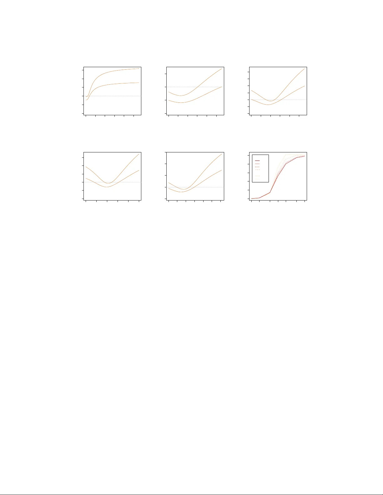
Regularized Laplacian Estimation and F ast Eigen vector A pproximation Patrick O. P erry Information, Operations, and Management Sciences NYU Stern School of Business New Y ork, NY 10012 pperry@stern.nyu.edu Michael W . Mahoney Department of Mathematics Stanford Univ ersity Stanford, CA 94305 mmahoney@cs.stanford.edu Abstract Recently , Mahoney and Orecchia demonstrated that popular diffusion-based pro- cedures to compute a quick appr oximation to the first nontrivial eigen vector of a data graph Laplacian exactly solve certain regularized Semi-Definite Programs (SDPs). In this paper , we extend that result by providing a statistical interpre- tation of their approximation procedure. Our interpretation will be analogous to the manner in which ` 2 -regularized or ` 1 -regularized ` 2 -regression (often called Ridge regression and Lasso regression, respectively) can be interpreted in terms of a Gaussian prior or a Laplace prior , respecti vely , on the coef ficient v ector of the regression problem. Our framew ork will imply that the solutions to the Mahoney- Orecchia regularized SDP can be interpreted as re gularized estimates of the pseu- doin verse of the graph Laplacian. Con versely , it will imply that the solution to this regularized estimation problem can be computed v ery quickly by running, e.g. , the fast diffusion-based PageRank procedure for computing an approximation to the first nontrivial eigen vector of the graph Laplacian. Empirical results are also provided to illustrate the manner in which approximate eigenv ector computation implicitly performs statistical regularization, relative to running the corresponding exact algorithm. 1 Introduction Approximation algorithms and heuristic approximations are commonly used to speed up the run- ning time of algorithms in machine learning and data analysis. In some cases, the outputs of these approximate procedures are “better” than the output of the more expensiv e exact algorithms, in the sense that they lead to more robust results or more useful results for the do wnstream practi- tioner . Recently , Mahoney and Orecchia formalized these ideas in the context of computing the first nontri vial eigen vector of a graph Laplacian [1]. Recall that, gi ven a graph G on n nodes or equiv alently its n × n Laplacian matrix L , the top nontri vial eigen vector of the Laplacian exactly op- timizes the Rayleigh quotient, subject to the usual constraints. This optimization problem can equi v- alently be expressed as a vector optimization program with the objective function f ( x ) = x T Lx , where x is an n -dimensional vector , or as a Semi-Definite Program (SDP) with objectiv e function F ( X ) = T r( LX ) , where X is an n × n symmetric positive semi-definite matrix. This first non- trivial v ector is, of course, of widespread interest in applications due to its usefulness for graph partitioning, image segmentation, data clustering, semi-supervised learning, etc. [2, 3, 4, 5, 6, 7]. In this conte xt, Mahone y and Orecchia asked the question: do popular dif fusion-based procedures— such as running the Heat Kernel or performing a Lazy Random W alk or computing the PageRank function—to compute a quick appr oximation to the first nontrivial eigenv ector of L solv e some other regularized version of the Rayleigh quotient objecti ve function e xactly ? Understanding this algorithmic-statistical tradeoff is clearly of interest if one is interested in very large-scale applica- tions, where performing statistical analysis to derive an objecti ve and then calling a black box solver to optimize that objectiv e exactly might be too expensi ve. Mahoney and Orecchia answered the abov e question in the af firmativ e, with the interesting twist that the regularization is on the SDP 1 formulation rather than the usual vector optimization problem. That is, these three diffusion-based procedures exactly optimize a regularized SDP with objectiv e function F ( X ) + 1 η G ( X ) , for some regularization function G ( · ) to be described below , subject to the usual constraints. In this paper, we extend the Mahone y-Orecchia result by providing a statistical interpretation of their approximation procedure. Our interpretation will be analogous to the manner in which ` 2 - regularized or ` 1 -regularized ` 2 -regression (often called Ridge regression and Lasso regression, respectiv ely) can be interpreted in terms of a Gaussian prior or a Laplace prior, respectiv ely , on the coefficient vector of the regression problem. In more detail, we will set up a sampling model, whereby the graph Laplacian is interpreted as an observ ation from a random process; we will posit the existence of a “population Laplacian” driving the random process; and we will then define an estimation problem: find the in verse of the population Laplacian. W e will show that the maximum a posteriori probability (MAP) estimate of the inv erse of the population Laplacian leads to a regular- ized SDP , where the objective function F ( X ) = T r( LX ) and where the role of the penalty function G ( · ) is to encode prior assumptions about the population Laplacian. In addition, we will show that when G ( · ) is the log-determinant function then the MAP estimate leads to the Mahoney-Orecchia regularized SDP corresponding to running the PageRank heuristic. Said another way , the solutions to the Mahoney-Orecchia regularized SDP can be interpreted as regularized estimates of the pseu- doin verse of the graph Laplacian. Moreov er , by Mahoney and Orecchia’ s main result, the solution to this regularized SDP can be computed very quickly—rather than solving the SDP with a black- box solver and rather computing explicitly the pseudoin verse of the Laplacian, one can simply run the fast diffusion-based PageRank heuristic for computing an approximation to the first nontri vial eigen vector of the Laplacian L . The next section describes some background. Section 3 then describes a statistical framework for graph estimation; and Section 4 describes prior assumptions that can be made on the population Laplacian. These two sections will shed light on the computational implications associated with these prior assumptions; b ut more importantly the y will shed light on the implicit prior assumptions associated with making certain decisions to speed up computations. Then, Section 5 will provide an empirical ev aluation, and Section 6 will provide a brief conclusion. Additional discussion is av ailable in the Appendix. 2 Background on Laplacians and diffusion-based pr ocedures A weighted symmetric graph G is defined by a v ertex set V = { 1 , . . . , n } , an edge set E ⊂ V × V , and a weight function w : E → R + , where w is assumed to be symmetric ( i.e . , w ( u, v ) = w ( v , u ) ). In this case, one can construct a matrix, L 0 ∈ R V × V , called the combinatorial Laplacian of G : L 0 ( u, v ) =  − w ( u, v ) when u 6 = v , d ( u ) − w ( u, u ) otherwise, where d ( u ) = P v w ( u, v ) is called the degree of u . By construction, L 0 is positive semidefinite. Note that the all-ones vector , often denoted 1 , is an eigen vector of L 0 with eigen value zero, i.e. , L 1 = 0 . For this reason, 1 is often called trivial eigen vector of L 0 . Letting D be a diagonal matrix with D ( u, u ) = d ( u ) , one can also define a normalized version of the Laplacian: L = D − 1 / 2 L 0 D − 1 / 2 . Unless explicitly stated otherwise, when we refer to the Laplacian of a graph, we will mean the normalized Laplacian. In many situations, e .g. , to perform spectral graph partitioning, one is interested in computing the first nontrivial eigen vector of a Laplacian. T ypically , this vector is computed “exactly” by calling a black-box solver; b ut it could also be approximated with an iteration-based method (such as the Power Method or Lanczos Method) or by running a random walk-based or diffusion-based method to the asymptotic state. These random walk-based or diffusion-based methods assign positive and negati ve “charge” to the nodes, and then the y let the distribution of charge evolv e according to dynamics deriv ed from the graph structure. Three canonical ev olution dynamics are the following: Heat Ker nel. Here, the charge ev olves according to the heat equation ∂ H t ∂ t = − LH t . Thus, the vector of charges ev olves as H t = exp( − tL ) = P ∞ k =0 ( − t ) k k ! L k , where t ≥ 0 is a time parameter , times an input seed distribution v ector . PageRank. Here, the charge at a node e volves by either moving to a neighbor of the current node or teleporting to a random node. More formally , the vector of char ges ev olves as R γ = γ ( I − (1 − γ ) M ) − 1 , (1) 2 where M is the natural random walk transition matrix associated with the graph and where γ ∈ (0 , 1) is the so-called teleportation parameter, times an input seed v ector . Lazy Random W alk. Here, the charge either stays at the current node or mov es to a neighbor . Thus, if M is the natural random walk transition matrix associated with the graph, then the vector of charges ev olves as some po wer of W α = αI + (1 − α ) M , where α ∈ (0 , 1) represents the “holding probability , ” times an input seed vector . In each of these cases, there is a parameter ( t , γ , and the number of steps of the Lazy Random W alk) that controls the “aggressiv eness” of the dynamics a nd thus how quickly the diffusi ve process equilibrates; and there is an input “seed” distrib ution vector . Thus, e.g. , if one is interested in global spectral graph partitioning, then this seed vector could be a vector with entries drawn from {− 1 , +1 } uniformly at random, while if one is interested in local spectral graph partitioning [8, 9, 10, 11], then this vector could be the indicator vector of a small “seed set” of nodes. See Appendix A for a brief discussion of local and global spectral partitioning in this context. Mahoney and Orecchia sho wed that these three dynamics arise as solutions to SDPs of the form minimize X T r( LX ) + 1 η G ( X ) subject to X  0 , T r( X ) = 1 , X D 1 / 2 1 = 0 , (2) where G is a penalty function (sho wn to be the generalized entropy , the log-determinant, and a certain matrix- p -norm, respecti vely [1]) and where η is a parameter related to the aggressiv eness of the diffusi ve process [1]. Con versely , solutions to the re gularized SDP of (2) for appropriate values of η can be computed exactly by running one of the abov e three diffusion-based procedures. Notably , when G = 0 , the solution to the SDP of (2) is uu 0 , where u is the smallest nontrivial eigen vector of L . More generally and in this precise sense, the Heat Kernel, PageRank, and Lazy Random W alk dynamics can be seen as “regularized” versions of spectral clustering and Laplacian eigen vector computation. Intuitively , the function G ( · ) is acting as a penalty function, in a manner analogous to the ` 2 or ` 1 penalty in Ridge regression or Lasso regression, and by running one of these three dynamics one is implicitly making assumptions about the form of G ( · ) . In this paper , we provide a statistical frame work to make that intuition precise. 3 A statistical framework f or regularized graph estimation Here, we will lay out a simple Bayesian framework for estimating a graph Laplacian. Importantly , this framew ork will allow for re gularization by incorporating prior information. 3.1 Analogy with regularized linear r egression It will be helpful to keep in mind the Bayesian interpretation of re gularized linear regression. In that context, we observe n predictor-response pairs in R p × R , denoted ( x 1 , y 1 ) , . . . , ( x n , y n ) ; the goal is to find a vector β such that β 0 x i ≈ y i . T ypically , we choose β by minimizing the residual sum of squares, i.e. , F ( β ) = RSS( β ) = P i k y i − β 0 x i k 2 2 , or a penalized version of it. For Ridge regression, we minimize F ( β ) + λ k β k 2 2 ; while for Lasso regression, we minimize F ( β ) + λ k β k 1 . The additional terms in the optimization criteria ( i.e. , λ k β k 2 2 and λ k β k 1 ) are called penalty func- tions; and adding a penalty function to the optimization criterion can often be interpreted as incor- porating prior information about β . F or example, we can model y 1 , . . . , y n as independent random observations with distributions dependent on β . Specifically , we can suppose y i is a Gaussian ran- dom variable with mean β 0 x i and known variance σ 2 . This induces a conditional density for the vector y = ( y 1 , . . . , y n ) : p ( y | β ) ∝ exp {− 1 2 σ 2 F ( β ) } , (3) where the constant of proportionality depends only on y and σ . Next, we can assume that β itself is random, drawn from a distribution with density p ( β ) . This distribution is called a prior , since it encodes prior knowledge about β . W ithout loss of generality , the prior density can be assumed to take the form p ( β ) ∝ exp {− U ( β ) } . (4) 3 Since the tw o random v ariables are dependent, upon observing y , we ha ve information about β . This information is encoded in the posterior density , p ( β | y ) , computed via Bayes’ rule as p ( β | y ) ∝ p ( y | β ) p ( β ) ∝ exp {− 1 2 σ 2 F ( β ) − U ( β ) } . (5) The MAP estimate of β is the v alue that maximizes p ( β | y ) ; equiv alently , it is the v alue of β that minimizes − log p ( β | y ) . In this frame work, we can recov er the solution to Ridge regres- sion or Lasso regression by setting U ( β ) = λ 2 σ 2 k β k 2 2 or U ( β ) = λ 2 σ 2 k β k 1 , respecti vely . Thus, Ridge regression can be interpreted as imposing a Gaussian prior on β , and Lasso re gression can be interpreted as imposing a double-exponential prior on β . 3.2 Bayesian infer ence for the population Laplacian For our problem, suppose that we have a connected graph with n nodes; or , equi valently , that we hav e L , the normalized Laplacian of that graph. W e will vie w this observed graph Laplacian, L , as a “sample” Laplacian, i.e. , as random object whose distribution depends on a true “population” Laplacian, L . As with the linear regression example, this induces a conditional density for L , to be denoted p ( L | L ) . Next, we can assume prior information about the population Laplacian in the form of a prior density , p ( L ) ; and, gi ven the observ ed Laplacian, we can estimate the population Laplacian by maximizing its posterior density , p ( L | L ) . Thus, to apply the Bayesian formalism, we need to specify the conditional density of L giv en L . In the context of linear regression, we assumed that the observations follo wed a Gaussian distribution. A graph Laplacian is not just a single observation—it is a positive semidefinite matrix with a very specific structure. Thus, we will take L to be a random object with expectation L , where L is another normalized graph Laplacian. Although, in general, L can be distinct from L , we will require that the nodes in the population and sample graphs have the same degrees. That is, if d =  d (1) , . . . , d ( n )  denotes the “degree v ector” of the graph, and D = diag  d (1) , . . . , d ( n )  , then we can define X = { X : X  0 , X D 1 / 2 1 = 0 , rank( X ) = n − 1 } , (6) in which case the population Laplacian and the sample Laplacian will both be members of X . T o model L , we will choose a distribution for positi ve semi-definite matrices analogous to the Gaussian distribution: a scaled W ishart matrix with expectation L . Note that, although it captures the trait that L is positiv e semi-definite, this distribution does not accurately model ev ery feature of L . For example, a scaled W ishart matrix does not necessarily have ones along its diagonal. Howe ver , the mode of the density is at L , a Laplacian; and for large values of the scale parameter , most of the mass will be on matrices close to L . Appendix B provides a more detailed heuristic justification for the use of the W ishart distribution. T o be more precise, let m ≥ n − 1 be a scale parameter , and suppose that L is distrib uted over X as a 1 m Wishart( L , m ) random v ariable. Then, E [ L | L ] = L , and L has conditional density p ( L | L ) ∝ exp {− m 2 T r( L L + ) } |L| m/ 2 , (7) where | · | denotes pseudodeterminant (product of nonzero eigenv alues). The constant of proportion- ality depends only on L , d , m , and n ; and we emphasize that the density is supported on X . Eqn. (7) is analogous to Eqn. (3) in the linear regression context, with 1 /m , the inv erse of the sample size parameter , playing the role of the variance parameter σ 2 . Next, suppose we hav e know that L is a random object drawn from a prior density p ( L ) . W ithout loss of generality , p ( L ) ∝ exp {− U ( L ) } , (8) for some function U , supported on a subset ¯ X ⊆ X . Eqn. (8) is analogous to Eqn. (4) from the linear regression e xample. Upon observing L , the posterior distribution for L is p ( L | L ) ∝ p ( L | L ) p ( L ) ∝ exp {− m 2 T r( L L + ) + m 2 log |L + | − U ( L ) } , (9) with support determined by ¯ X . Eqn. (9) is analogous to Eqn. (5) from the linear regression example. If we denote by ˆ L the MAP estimate of L , then it follo ws that ˆ L + is the solution to the program minimize X T r( LX ) + 2 m U ( X + ) − log | X | subject to X ∈ ¯ X ⊆ X . (10) 4 Note the similarity with Mahone y-Orecchia regularized SDP of (2). In particular , if ¯ X = { X : T r( X ) = 1 } ∩ X , then the two programs are identical except for the factor of log | X | in the opti- mization criterion. 4 A prior related to the P ageRank procedur e Here, we will present a prior distribution for the population Laplacian that will allow us to lev erage the estimation frame work of Section 3; and we will show that the MAP estimate of L for this prior is related to the P ageRank procedure via the Mahoney-Orecchia regularized SDP . Appendix C presents priors that lead to the Heat Kernel and Lazy Random W alk in an analogous way; in both of these cases, howe ver , the priors are data-dependent in the strong sense that they explicitly depend on the number of data points. 4.1 Prior density The prior we will present will be based on neutrality and inv ariance conditions; and it will be sup- ported on X , i.e. , on the subset of positive-semidefinite matrices that was the support set for the conditional density defined in Eqn. (7). In particular , recall that, in addition to being positi ve semi- definite, e very matrix in the support set has rank n − 1 and satisfies X D 1 / 2 1 = 0 . Note that because the prior depends on the data (via the orthogonality constraint induced by D ), this is not a prior in the fully Bayesian sense; instead, the prior can be considered as part of an empirical or pseudo-Bayes estimation procedure. The prior we will specify depends only on the eigenv alues of the normalized Laplacian, or equiv a- lently on the eigen values of the pseudoin verse of the Laplacian. Let L + = τ O Λ O 0 be the spectral decomposition of the pseudoinv erse of the normalized Laplacian L , where τ ≥ 0 is a scale factor , O ∈ R n × n − 1 is an orthogonal matrix, and Λ = diag  λ (1) , . . . , λ ( n − 1)  , where P v λ ( v ) = 1 . Note that the v alues λ (1) , . . . , λ ( n − 1) are unordered and that the vector λ =  λ (1) , . . . , λ ( n − 1)  lies in the unit simplex. If we require that the distrib ution for λ be exchangeable (in variant under permutations) and neutral ( λ ( v ) independent of the vector  λ ( u ) / (1 − λ ( v )) : u 6 = v  , for all v ), then the only non-degenerate possibility is that λ is Dirichlet-distributed with parameter vector ( α, . . . , α ) [12]. The parameter α , to which we refer as the “shape” parameter , must satisfy α > 0 for the density to be defined. In this case, p ( L ) ∝ p ( τ ) n − 1 Y v =1 λ ( v ) α − 1 , (11) where p ( τ ) is a prior for τ . Thus, the prior weight on L only depends on τ and Λ . One implication is that the prior is “nearly” rotationally in variant, in the sense that p ( P 0 L P ) = p ( L ) for any rank- ( n − 1) projection matrix P satisfying P D 1 / 2 1 = 0 . 4.2 Posterior estimation and connection to P ageRank T o analyze the MAP estimate associated with the prior of Eqn. (11) and to explain its connection with the PageRank dynamics, the follo wing proposition is crucial. Proposition 4.1. Suppose the conditional likelihood for L given L is as defined in (7) and the prior density for L is as defined in (11) . Define ˆ L to be the MAP estimate of L . Then, [T r( ˆ L + )] − 1 ˆ L + solves the Mahone y-Or ecchia r e gularized SDP (2) , with G ( X ) = − log | X | and η as given in Eqn. (12) below . Pr oof. For L in the support set of the posterior , define τ = T r( L + ) and Θ = τ − 1 L + , so that T r(Θ) = 1 . Further , rank(Θ) = n − 1 . Express the prior in the form of Eqn. (8) with function U giv en by U ( L ) = − log { p ( τ ) | Θ | α − 1 } = − ( α − 1) log | Θ | − log p ( τ ) , where, as before, | · | denotes pseudodeterminant. Using (9) and the relation |L + | = τ n − 1 | Θ | , the posterior density for L gi ven L is p ( L | L ) ∝ exp n − mτ 2 T r( L Θ) + m +2( α − 1) 2 log | Θ | + g ( τ ) o , 5 where g ( τ ) = m ( n − 1) 2 log τ + log p ( τ ) . Suppose ˆ L maximizes the posterior lik elihood. Define ˆ τ = T r( ˆ L + ) and ˆ Θ = [ ˆ τ ] − 1 ˆ L + . In this case, ˆ Θ must minimize the quantity T r( L ˆ Θ) − 1 η log | ˆ Θ | , where η = m ˆ τ m + 2( α − 1) . (12) Thus ˆ Θ solves the re gularized SDP (2) with G ( X ) = − log | X | . Mahoney and Orecchia sho wed that the solution to (2) with G ( X ) = − log | X | is closely related to the PageRank matrix, R γ , defined in Eqn. (1). By combining Proposition 4.1 with their result, we get that the MAP estimate of L satisfies ˆ L + ∝ D − 1 / 2 R γ D 1 / 2 ; con versely , R γ ∝ D 1 / 2 ˆ L + D − 1 / 2 . Thus, the PageRank operator of Eqn. (1) can be viewed as a degree-scaled regularized estimate of the pseudoinv erse of the Laplacian. Moreover , prior assumptions about the spectrum of the graph Laplacian ha ve direct implications on the optimal teleportation parameter . Specifically Mahoney and Orecchia’ s Lemma 2 sho ws how η is related to the teleportation parameter γ , and Eqn. (12) shows ho w the optimal η is related to prior assumptions about the Laplacian. 5 Empirical ev aluation In this section, we provide an empirical ev aluation of the performance of the regularized Laplacian estimator , compared with the unregularized estimator . T o do this, we need a ground truth population Laplacian L and a noisily-observed sample Laplacian L . Thus, in Section 5.1, we construct a family of distributions for L ; importantly , this f amily will be able to represent both lo w-dimensional graphs and expander -like graphs. Interestingly , the prior of Eqn. (11) captures some of the qualitati ve features of both of these types of graphs (as the shape parameter is varied). Then, in Section 5.2, we describe a sampling procedure for L which, superficially , has no relation to the scaled W ishart conditional density of Eqn. (7). Despite this model misspecification, the regularized estimator ˆ L η outperforms L for many choices of the re gularization parameter η . 5.1 Ground truth generation and prior e valuation The ground truth graphs we generate are motiv ated by the W atts-Strogatz “small-world” model [13]. T o generate a ground truth population Laplacian, L —equiv alently , a population graph—we start with a two-dimensional lattice of width w and height h , and thus n = w h nodes. Points in the lattice are connected to their four nearest neighbors, making adjustments as necessary at the boundary . W e then perform s edge-swaps: for each sw ap, we choose two edges uniformly at random and then we swap the endpoints. For example, if we sample edges i 1 ∼ j 1 and i 2 ∼ j 2 , then we replace these edges with i 1 ∼ j 2 and i 2 ∼ j 1 . Thus, when s = 0 , the graph is the original discretization of a low-dimensional space; and as s increases to infinity , the graph becomes more and more like a uniformly chosen 4 -re gular graph (which is an expander [14] and which bears similarities with an Erd ˝ os-R ´ enyi random graph [15]). Indeed, each edge swap is a step of the Metropolis algorithm tow ard a uniformly chosen random graph with a fixed degree sequence. For the empirical ev aluation presented here, h = 7 and w = 6 ; but the results are qualitati vely similar for other values. Figure 1 compares the expected order statistics (sorted values) for the Dirichlet prior of Eqn. (11) with the e xpected eigen values of Θ = L + / T r( L + ) for the small-world model. In particular , in Figure 1(a), we show the behavior of the order statistics of a Dirichlet distribution on the ( n − 1) - dimensional simplex with scalar shape parameter α , as a function of α . For each value of the shape α , we generated a random ( n − 1) -dimensional Dirichlet vector , λ , with parameter vector ( α, . . . , α ) ; we computed the n − 1 order statistics of λ by sorting its components; and we repeated this procedure for 500 replicates and av eraged the values. Figure 1(b) shows a corresponding plot for the ordered eigen values of Θ . For each value of s (normalized, here, by the number of edges µ , where µ = 2 w h − w − h = 71 ), we generated the normalized Laplacian, L , corresponding to the random s -edge-swapped grid; we computed the n − 1 nonzero eigen values of Θ ; and we performed 1000 replicates of this procedure and av eraged the resulting eigen values. Interestingly , the behavior of the spectrum of the small-world model as the edge-swaps increase is qualitativ ely quite similar to the behavior of the Dirichlet prior order statistics as the shape param- eter α increases. In particular , note that for small values of the shape parameter α the first few order-statistics are well-separated from the rest; and that as α increases, the order statistics become 6 0.5 1.0 1.5 2.0 0.00 0.10 0.20 Shape Order statistics ● ● ● ● ● ● ● ● ● ● ● ● ● ● ● ● ● ● ● ● ● ● ● ● ● ● ● ● ● ● ● ● ● ● ● ● ● ● ● ● ● ● ● ● ● ● ● ● ● ● ● ● ● ● ● ● ● ● ● ● ● ● ● ● ● ● ● ● ● ● ● ● ● ● ● ● ● ● ● ● ● ● ● ● ● ● ● ● ● ● ● ● ● ● ● ● ● ● ● ● ● ● ● ● ● ● ● ● ● ● ● ● ● ● ● ● ● ● ● ● ● ● ● ● ● ● ● ● ● ● ● ● ● ● ● ● ● ● ● ● ● ● ● ● ● ● ● ● ● ● ● ● ● ● ● ● ● ● ● ● ● ● ● ● ● ● ● ● ● ● ● ● ● ● ● ● ● ● ● ● ● ● ● ● ● ● ● ● ● ● ● ● ● ● ● ● ● ● ● ● ● ● ● ● ● ● ● ● ● ● ● ● ● ● ● ● ● ● ● ● ● ● ● ● ● ● ● ● ● ● ● ● ● ● ● ● ● ● ● ● ● ● ● ● ● ● ● ● ● ● ● ● ● ● ● ● ● ● ● ● ● ● ● ● ● ● ● ● ● ● ● ● ● ● ● ● ● ● ● ● ● ● ● ● ● ● ● ● ● ● ● ● ● ● ● ● ● ● ● ● ● ● ● ● ● ● ● ● ● ● ● ● ● ● ● ● ● ● ● ● ● ● ● ● ● ● ● ● ● ● ● ● ● ● ● ● ● ● ● ● ● ● ● ● ● ● ● ● ● ● ● ● ● ● ● ● ● ● ● ● ● ● ● ● ● ● ● ● ● ● ● ● ● ● ● ● ● ● ● ● ● ● ● ● ● ● ● ● ● ● ● ● ● ● ● ● ● ● ● ● ● ● ● ● ● ● ● ● ● ● ● ● ● ● ● ● ● ● ● ● ● ● ● ● ● ● ● ● ● ● ● ● ● ● ● ● ● ● ● ● ● ● ● ● ● ● ● ● ● ● ● ● ● ● ● ● ● ● ● ● ● ● ● ● ● ● ● ● ● ● ● ● ● ● ● ● ● ● ● ● ● ● ● ● ● ● ● ● ● ● ● ● ● ● ● ● ● ● ● ● ● ● ● ● ● ● ● ● ● ● ● ● ● ● ● ● ● ● ● ● ● ● ● ● ● ● ● ● ● ● ● ● ● ● ● ● ● ● ● ● ● ● ● ● ● ● ● ● ● ● ● ● ● ● ● ● ● ● ● ● ● ● ● ● ● ● ● ● ● ● ● ● ● ● ● ● ● ● ● ● ● ● ● ● ● ● ● ● ● ● ● ● ● ● ● ● ● ● ● ● ● ● ● ● ● ● ● ● ● ● ● ● ● ● ● ● ● ● ● ● ● ● ● ● ● ● ● ● ● ● ● ● ● ● ● ● ● ● ● ● ● ● ● ● ● ● ● ● ● ● ● ● ● ● ● ● (a) Dirichlet distrib ution order statistics. 0.0 0.2 0.4 0.6 0.8 1.0 0.00 0.05 0.10 0.15 0.20 Swaps Edges Inv erse Laplacian Eigenvalues ● ● ● ● ● ● ● ● ● ● ● ● ● ● ● ● ● ● ● ● ● ● ● ● ● ● ● ● ● ● ● ● ● ● ● ● ● ● ● ● ● ● ● ● ● ● ● ● ● ● ● ● ● ● ● ● ● ● ● ● ● ● ● ● ● ● ● ● ● ● ● ● ● ● ● ● ● ● ● ● ● ● ● ● ● ● ● ● ● ● ● ● ● ● ● ● ● ● ● ● ● ● ● ● ● ● ● ● ● ● ● ● ● ● ● ● ● ● ● ● ● ● ● ● ● ● ● ● ● ● ● ● ● ● ● ● ● ● ● ● ● ● ● ● ● ● ● ● ● ● ● ● ● ● ● ● ● ● ● ● ● ● ● ● ● ● ● ● ● ● ● ● ● ● ● ● ● ● ● ● ● ● ● ● ● ● ● ● ● ● ● ● ● ● ● ● ● ● ● ● ● ● ● ● ● ● ● ● ● ● ● ● ● ● ● ● ● ● ● ● ● ● ● ● ● ● ● ● ● ● ● ● ● ● ● ● ● ● ● ● ● ● ● ● ● ● ● ● ● ● ● ● ● ● ● ● ● ● ● ● ● ● ● ● ● ● ● ● ● ● ● ● ● ● ● ● ● ● ● ● ● ● ● ● ● ● ● ● ● ● ● ● ● ● ● ● ● ● ● ● ● ● ● ● ● ● ● ● ● ● ● ● ● ● ● ● ● ● ● ● ● ● ● ● ● ● ● ● ● ● ● ● ● ● ● ● ● ● ● ● ● ● ● ● ● ● ● ● ● ● ● ● ● ● ● ● ● ● ● ● ● ● ● ● ● ● ● ● ● ● ● ● ● ● ● ● ● ● ● ● ● ● ● ● ● ● ● ● ● ● ● ● ● ● ● ● ● ● ● ● ● ● ● ● ● ● ● ● ● ● ● ● ● ● ● ● ● ● ● ● ● ● ● ● ● ● ● ● ● ● ● ● ● ● ● ● ● ● ● ● ● ● ● ● ● ● ● ● ● ● ● ● ● ● ● ● ● ● ● ● ● ● ● ● ● ● ● ● ● ● ● ● ● ● ● ● ● ● ● ● ● ● ● ● ● ● ● ● ● ● ● ● ● ● ● ● ● ● ● ● ● ● ● ● ● ● ● ● ● ● ● ● ● ● ● ● ● ● ● ● ● ● ● ● ● ● ● ● ● ● ● ● ● ● ● ● ● ● ● ● ● ● ● ● ● ● ● ● ● ● ● ● ● ● ● ● ● ● ● ● ● ● ● ● ● ● ● ● ● ● ● ● ● ● ● ● ● ● ● ● ● ● ● ● ● ● ● ● ● ● ● ● ● ● ● ● ● ● ● ● ● ● ● ● ● ● ● ● ● ● ● ● ● ● ● ● ● ● ● ● ● ● ● ● ● ● ● ● ● ● ● ● ● ● ● ● ● ● ● ● ● ● ● ● ● ● ● ● ● ● ● ● ● ● ● ● ● ● ● ● ● ● ● ● ● ● ● ● ● ● ● ● ● ● ● ● ● ● ● ● ● ● ● ● ● ● ● ● ● ● ● ● ● ● ● ● ● (b) Spectrum of the in verse Laplacian. Figure 1: Analytical and empirical priors. 1(a) shows the Dirichlet distribution order statistics versus the shape parameter; and 1(b) shows the spectrum of Θ as a function of the rewiring parameter . concentrated around 1 / ( n − 1) . Similarly , when the edge-swap parameter s = 0 , the top two eigen- values (corresponding to the width-wise and height-wise coordinates on the grid) are well-separated from the bulk; as s increases, the top eigenv alues quickly merge into the b ulk; and ev entually , as s goes to infinity , the distrib ution becomes very close that that of a uniformly chosen 4 -regular graph. 5.2 Sampling procedur e, estimation performance, and optimal r egularization behavior Finally , we e v aluate the estimation performance of a regularized estimator of the graph Laplacian and compare it with an unregularized estimate. T o do so, we construct the population graph G and its Laplacian L , for a gi ven value of s , as described in Section 5.1. Let µ be the number of edges in G . The sampling procedure used to generate the observed graph G and its Laplacian L is parameterized by the sample size m . (Note that this parameter is analogous to the W ishart scale parameter in Eqn. (7), but here we are sampling from a different distribution.) W e randomly choose m edges with replacement from G ; and we define sample graph G and corresponding Laplacian L by setting the weight of i ∼ j equal to the number of times we sampled that edge. Note that the sample graph G ov er-counts some edges in G and misses others. W e then compute the regularized estimate ˆ L η , up to a constant of proportionality , by solving (implic- itly!) the Mahone y-Orecchia re gularized SDP (2) with G ( X ) = − log | X | . W e define the unre gular- ized estimate ˆ L to be equal to the observ ed Laplacian, L . Giv en a population Laplacian L , we define τ = τ ( L ) = T r( L + ) and Θ = Θ( L ) = τ − 1 L + . W e define ˆ τ η , ˆ τ , ˆ Θ η , and ˆ Θ similarly to the popu- lation quantities. Our performance criterion is the relativ e Frobenius error k Θ − ˆ Θ η k F / k Θ − ˆ Θ k F , where k · k F denotes the Frobenius norm ( k A k F = [T r( A 0 A )] 1 / 2 ). Appendix D presents similar results when the performance criterion is the relativ e spectral norm error . Figures 2(a), 2(b), and 2(c) sho w the regularization performance when s = 4 (an intermediate value) for three different values of m/µ . In each case, the mean error and one standard de viation around it are plotted as a function of η/ ¯ τ , as computed from 100 replicates; here, ¯ τ is the mean value of τ over all replicates. The implicit regularization clearly improves the performance of the estimator for a large range of η values. (Note that the regularization parameter in the regularized SDP (2) is 1 /η , and thus smaller values along the X-axis correspond to stronger regularization.) In particular , when the data are very noisy , e.g. , when m/µ = 0 . 2 , as in Figure 2(a), improv ed results are seen only for very strong regularization; for intermediate lev els of noise, e.g . , m/µ = 1 . 0 , as in Figure 2(b), (in which case m is chosen such that G and G have the same number of edges counting multiplicity), improv ed performance is seen for a wide range of v alues of η ; and for lo w le vels of noise, Figure 2(c) illustrates that improved results are obtained for moderate lev els of implicit regularization. Figures 2(d) and 2(e) illustrate similar results for s = 0 and s = 32 . 7 0.0 0.5 1.0 1.5 2.0 2.5 0.0 0.5 1.0 1.5 2.0 2.5 Regularization Rel. Frobenius Error ● ● ● ● ● ● ● ● ● ● ● ● ● ● ● ● ● ● ● ● ● ● ● ● ● ● ● ● ● ● ● ● ● ● ● ● ● ● ● ● ● ● ● ● ● ● ● ● ● ● ● ● ● ● ● ● ● ● ● ● ● ● ● ● ● ● ● ● ● ● ● ● ● ● ● ● ● ● ● ● ● ● ● ● ● ● ● ● ● ● ● ● ● ● ● ● ● ● ● ● (a) m/µ = 0 . 2 and s = 4 . 0.0 0.5 1.0 1.5 2.0 2.5 0.0 0.5 1.0 1.5 Regularization Rel. Frobenius Error ● ● ● ● ● ● ● ● ● ● ● ● ● ● ● ● ● ● ● ● ● ● ● ● ● ● ● ● ● ● ● ● ● ● ● ● ● ● ● ● ● ● ● ● ● ● ● ● ● ● ● ● ● ● ● ● ● ● ● ● ● ● ● ● ● ● ● ● ● ● ● ● ● ● ● ● ● ● ● ● ● ● ● ● ● ● ● ● ● ● ● ● ● ● ● ● ● ● ● ● (b) m/µ = 1 . 0 and s = 4 . 0.0 0.5 1.0 1.5 2.0 2.5 0.0 0.5 1.0 1.5 2.0 2.5 3.0 Regularization Rel. Frobenius Error ● ● ● ● ● ● ● ● ● ● ● ● ● ● ● ● ● ● ● ● ● ● ● ● ● ● ● ● ● ● ● ● ● ● ● ● ● ● ● ● ● ● ● ● ● ● ● ● ● ● ● ● ● ● ● ● ● ● ● ● ● ● ● ● ● ● ● ● ● ● ● ● ● ● ● ● ● ● ● ● ● ● ● ● ● ● ● ● ● ● ● ● ● ● ● ● ● ● ● ● (c) m/µ = 2 . 0 and s = 4 . 0.0 0.5 1.0 1.5 2.0 2.5 0.0 0.5 1.0 1.5 2.0 2.5 Regularization Rel. Frobenius Error ● ● ● ● ● ● ● ● ● ● ● ● ● ● ● ● ● ● ● ● ● ● ● ● ● ● ● ● ● ● ● ● ● ● ● ● ● ● ● ● ● ● ● ● ● ● ● ● ● ● ● ● ● ● ● ● ● ● ● ● ● ● ● ● ● ● ● ● ● ● ● ● ● ● ● ● ● ● ● ● ● ● ● ● ● ● ● ● ● ● ● ● ● ● ● ● ● ● ● ● (d) m/µ = 2 . 0 and s = 0 . 0.0 0.5 1.0 1.5 2.0 2.5 3.0 0 1 2 3 4 Regularization Rel. Frobenius Error ● ● ● ● ● ● ● ● ● ● ● ● ● ● ● ● ● ● ● ● ● ● ● ● ● ● ● ● ● ● ● ● ● ● ● ● ● ● ● ● ● ● ● ● ● ● ● ● ● ● ● ● ● ● ● ● ● ● ● ● ● ● ● ● ● ● ● ● ● ● ● ● ● ● ● ● ● ● ● ● ● ● ● ● ● ● ● ● ● ● ● ● ● ● ● ● ● ● ● ● (e) m/µ = 2 . 0 and s = 32 . 0.1 0.2 0.5 1.0 2.0 5.0 10.0 0.0 0.2 0.4 0.6 0.8 1.0 Sample Proportion Optimal Penalty ● ● ● ● ● ● ● ● ● ● ● ● ● ● ● ● ● ● ● ● ● ● ● ● ● ● ● ● ● ● ● ● ● ● ● ● ● ● ● ● ● ● ● ● ● ● ● ● ● Swaps/Edges 0.90 0.45 0.23 0.11 0.06 0.03 0.01 (f) Optimal η ∗ / ¯ τ . Figure 2: Regularization performance. 2(a) through 2(e) plot the relati ve Frobenius norm error, versus the (normalized) re gularization parameter η / ¯ τ . Shown are plots for various v alues of the (normalized) number of edges, m/µ , and the edge-swap parameter , s . Recall that the regularization parameter in the re gularized SDP (2) is 1 /η , and thus smaller v alues along the X-axis correspond to stronger re gularization. 2(f) plots the optimal regularization parameter η ∗ / ¯ τ as a function of sample proportion for different fractions of edge sw aps. As when regularization is implemented explicitly , in all these cases, we observ e a “sweet spot” where there is an optimal v alue for the implicit re gularization parameter . Figure 2(f) illustrates how the optimal choice of η depends on parameters defining the population Laplacians and sample Laplacians. In particular, it illustrates how η ∗ , the optimal value of η (normalized by ¯ τ ), depends on the sampling proportion m/µ and the swaps per edges s/µ . Observe that as the sample size m increases, η ∗ con ver ges monotonically to ¯ τ ; and, further, that higher values of s (corresponding to more e xpander-like graphs) correspond to higher v alues of η ∗ . Both of these observations are in direct agreement with Eqn. (12). 6 Conclusion W e hav e provided a statistical interpretation for the observation that popular diffusion-based proce- dures to compute a quick approximation to the first nontri vial eigenv ector of a data graph Laplacian exactly solve a certain re gularized version of the problem. One might be tempted to vie w our re- sults as “unfortunate, ” in that it is not straightforward to interpret the priors presented in this paper . Instead, our results should be viewed as making explicit the implicit prior assumptions associated with making certain decisions (that are alr eady made in practice) to speed up computations. Sev eral extensions suggest themselves. The most obvious might be to try to obtain Proposition 4.1 with a more natural or empirically-plausible model than the W ishart distribution; to extend the em- pirical e valuation to much larger and more realistic data sets; to apply our methodology to other widely-used approximation procedures; and to characterize when implicitly regularizing an eigen- vector leads to better statistical beha vior in do wnstream applications where that eigenv ector is used. More generally , though, we expect that understanding the algorithmic-statistical tradeof fs that we hav e illustrated will become increasingly important in very large-scale data analysis applications. 8 References [1] M. W . Mahoney and L. Orecchia. Implementing re gularization implicitly via approximate eigen vector computation. In Pr oceedings of the 28th International Confer ence on Mac hine Learning , pages 121–128, 2011. [2] D.A. Spielman and S.-H. T eng. Spectral partitioning works: Planar graphs and finite element meshes. In FOCS ’96: Pr oceedings of the 37th Annual IEEE Symposium on F oundations of Computer Science , pages 96–107, 1996. [3] S. Guattery and G.L. Miller . On the quality of spectral separators. SIAM Journal on Matrix Analysis and Applications , 19:701–719, 1998. [4] J. Shi and J. Malik. Normalized cuts and image segmentation. IEEE T ranscations of P attern Analysis and Machine Intelligence , 22(8):888–905, 2000. [5] M. Belkin and P . Niyogi. Laplacian eigenmaps for dimensionality reduction and data repre- sentation. Neural Computation , 15(6):1373–1396, 2003. [6] T . Joachims. Transducti ve learning via spectral graph partitioning. In Pr oceedings of the 20th International Confer ence on Machine Learning , pages 290–297, 2003. [7] J. Leskov ec, K.J. Lang, A. Dasgupta, and M.W . Mahoney . Community structure in large networks: Natural cluster sizes and the absence of large well-defined clusters. Internet Math- ematics , 6(1):29–123, 2009. Also av ailable at: [8] D.A. Spielman and S.-H. T eng. Nearly-linear time algorithms for graph partitioning, graph sparsification, and solving linear systems. In STOC ’04: Pr oceedings of the 36th annual A CM Symposium on Theory of Computing , pages 81–90, 2004. [9] R. Andersen, F .R.K. Chung, and K. Lang. Local graph partitioning using PageRank vectors. In FOCS ’06: Pr oceedings of the 47th Annual IEEE Symposium on F oundations of Computer Science , pages 475–486, 2006. [10] F .R.K. Chung. The heat kernel as the pagerank of a graph. Pr oceedings of the National Academy of Sciences of the United States of America , 104(50):19735–19740, 2007. [11] M. W . Mahoney , L. Orecchia, and N. K. V ishnoi. A spectral algorithm for improving graph partitions with applications to exploring data graphs locally . T echnical report. Preprint: arXiv:0912.0681 (2009). [12] J. Fabius. T wo characterizations of the Dirichlet distribution. The Annals of Statistics , 1(3):583–587, 1973. [13] D.J. W atts and S.H. Strogatz. Collective dynamics of small-world networks. Natur e , 393:440– 442, 1998. [14] S. Hoory , N. Linial, and A. W igderson. Expander graphs and their applications. Bulletin of the American Mathematical Society , 43:439–561, 2006. [15] B. Bollobas. Random Graphs . Academic Press, London, 1985. [16] W .E. Donath and A.J. Hoffman. Lo wer bounds for the partitioning of graphs. IBM Journal of Resear ch and Development , 17:420–425, 1973. [17] M. Fiedler . A property of eigen vectors of nonnegativ e symmetric matrices and its application to graph theory . Czechoslovak Mathematical J ournal , 25(100):619–633, 1975. [18] M. Mihail. Conductance and con ver gence of Markov chains—a combinatorial treatment of expanders. In Pr oceedings of the 30th Annual IEEE Symposium on F oundations of Computer Science , pages 526–531, 1989. [19] P . Y u. Chebotarev and E. V . Shamis. On proximity measures for graph vertices. A utomation and Remote Contr ol , 59(10):1443–1459, 1998. [20] A. K. Chandra, P . Ragha van, W . L. Ruzzo, R. Smolensk y , and P . T iwari. The electrical re- sistance of a graph captures its commute and cover times. In Pr oceedings of the 21st Annual A CM Symposium on Theory of Computing , pages 574–586, 1989. 9 A Relationship with local and global spectral graph partitioning In this section, we briefly describe the connections between our results and global and local v ersions of spectral partitioning, which were a starting point for this work. The idea of spectral clustering is to approximate the best partition of the v ertices of a connected graph into two pieces by using the nontrivial eigen vectors of a Laplacian (either the combinatorial or the normalized Laplacian). This idea has had a long history [16, 17, 2, 3, 4]. The simplest version of spectral clustering in volves computing the first nontrivial eigen vector (or another vector with Rayleigh quotient close to that of the first nontrivial eigenv ector) of L , and “sweeping” o ver that vector . For e xample, one can take that vector , call it x , and, for a given threshold K , define the two sets of the partition as C ( x, K ) = { i : x i ≥ K } , and ¯ C ( x, K ) = { i : x i < K } . T ypically , this vector x is computed by calling a black-box solver , but it could also be approximated with an iteration-based method (such as the Power Method or Lanczos Method) or a random walk- based method (such as running a diffusi ve procedure or PageRank-based procedure to the asymptotic state). Far from being a “heuristic, ” this procedure pro vides a global partition that (via Cheeger’ s in- equality and for an appropriate choice of K ) satisfies prov able quality-of-approximation guarantees with respect to the combinatorial optimization problem of finding the best “conductance” partition in the entire graph [18, 2, 3]. Although spectral clustering reduces a graph to a single vector —the smallest nontri vial eigenv ector of the graph’ s Laplacian—and then clusters the nodes using the information in that vector , it is pos- sible to obtain much more information about the graph by looking at more than one eigen vector of the Laplacian. In particular , the elements of the pseudoinv erse of the combinatorial Laplacian, L + 0 , giv e local ( i.e. , node-specific) information about random walks on the graph. The reason is that the pseudoin verse L + 0 of the Laplacian is closely related to random w alks on the graph. See, e.g . [19] for details. For example, it is known that the quantity L + 0 ( u, u ) + L + 0 ( v , v ) − L + 0 ( u, v ) − L + 0 ( v , u ) is pro- portional to the commute time, a symmetrized version of the length of time before a random walker started at node u reaches node v , whene ver u and v are in the same connected component [20]. Simi- larly , the elements of the pseudoin verse of the normalized Laplacian gi ve degree-scaled measures of proximity between the nodes of a graph. It is likely that L + ( u, v ) has a probabilistic interpretation in terms of random walks on the graph, along the lines of our methodology , but we are not aware of any such interpretation. From this perspective, giv en L + and a cutoff value, K , we can define a local partition around node u via P K ( u ) = { v : L + ( u, v ) > K } . (Note that if v is in P K ( u ) , then u is in P K ( v ) ; in addition, if the graph is disconnected, then there exists a K such that u and v are in the same connected component iff v ∈ P K ( u ) .) W e call clustering procedures based on this idea local spectral partitioning . Although the na ¨ ıve way of performing this local spectral partitioning, i.e . , to compute L + explicitly , is prohibiti ve for anything but v ery small graphs, these ideas form the basis for very fast local spectral clustering methods that employ truncated diffusion-based procedures to compute localized vectors with which to partition. For example, this idea can be implemented by performing a dif fusion- based procedure with an input seed distribution v ector localized on a node u and then sweeping ov er the resulting vector . This idea was originally introduced in [8] as a dif fusion-based operational procedure that was local in a very strong sense and that led to Cheeger -like bounds analogous to those obtained with the usual global spectral partitioning; and this was extended and improved by [9, 10]. In addition, an optimization perspective on this was provided by [11]. Although [11] is local in a weaker sense, it does obtain local Cheeger -like guarantees from an explicit locally-biased optimization problem, and it pro vides an optimization ansatz that may be interpreted as a “local eigen vector . ” See [8, 9, 10, 11] for details. Understanding the relationship between the “operational procedure versus optimization ansatz” perspecti ves was the origin of [1] and thus of this w ork. B Heuristic justification f or the Wishart density In this section, we describe a sampling procedure for L which, in a very crude sense, leads approxi- mately to a conditional W ishart density for p ( L | L ) . Let G be a graph with vertex set V = { 1 , 2 , . . . , n } , edge set E = V × V equipped with the equiv alence relation ( u, v ) = ( v , u ) . Let ω be an edge weight function, and let L 0 and L be 10 the corresponding combinatorial and normalized Laplacians. Let ∆ be a diagonal matrix with ∆( u, u ) = P v ω ( u, v ) , so that L = ∆ − 1 / 2 L 0 ∆ − 1 / 2 . Suppose the weights are scaled such that P ( u,v ) ∈ E ω ( u, v ) = 1 , and suppose further that ∆( u, u ) > 0 . W e refer to ω ( u, v ) as the population weight of edge ( u, v ) . A simple model for the sample graph is as follows: we sample m edges from E , randomly chosen according to the population weight function. That is, we see edges ( u 1 , v 1 ) , ( u 2 , v 2 ) , . . . , ( u m , v m ) , where the edges are all dra wn independently and identically such that the probability of seeing edge ( u, v ) is determined by ω : P ω { ( u 1 , v 1 ) = ( u, v ) } = ω ( u, v ) . Note that we will likely see duplicate edges and not every edge with a positi ve weight will get sampled. Then, we construct a weight function from the sampled edges, called the sample weight function, w , defined such that w ( u, v ) = 1 m m X i =1 1 { ( u i , v i ) = ( u, v ) } , where 1 {·} is an indicator vector . In turn, we construct a sample combinatorial Laplacian, L 0 , defined such that L 0 ( u, v ) =  P w w ( u, w ) when u = v , − w ( u, v ) otherwise. Let D be a diagonal matrix such that D ( u, u ) = P v w ( u, v ) , and define L = D − 1 / 2 L 0 D − 1 / 2 . Let- ting E ω denote expectation with respect to the probability law P ω , note that E ω [ w ( u, v )] = ω ( u, v ) , that E ω L 0 = L 0 , and that E ω D = ∆ . Moreover , the strong law of large numbers guarantees that as m increases, these three quantities con verge almost surely to their expectations. Further , Slutzky’ s theorem guarantees that √ m ( L − L ) and √ m ∆ − 1 / 2 ( L 0 − L 0 )∆ − 1 / 2 con ver ge in distribution to the same limit. W e use this large-sample behavior to approximate the the distribution of L by the distribution of ∆ − 1 / 2 L 0 ∆ − 1 / 2 . Put simply , we treat the degrees as kno wn. The distrib ution of L 0 is completely determined by the edge sampling scheme laid out abov e. How- ev er , the exact form for the density inv olves an intractable combinatorial sum. Thus, we appeal to a crude approximation for the conditional density . The approximation works as follo ws: 1. For i = 1 , . . . , m , define x i ∈ R n such that x i ( u ) =    + s i when u = u i , − s i when u = v i , 0 otherwise, where s i ∈ {− 1 , +1 } is chosen arbitrarily . Note that L 0 = 1 m P m i =1 x i x 0 i . 2. T ake s i to be random, equal to +1 or − 1 with probability 1 2 . Approximate the distribution of x i by the distribution of a multiv ariate normal random v ariable, ˜ x i , such that x i and ˜ x i hav e the same first and second moments. 3. Approximate the distribution of L 0 by the distribution of ˜ L 0 , where ˜ L 0 = 1 m P m i =1 ˜ x i ˜ x 0 i . 4. Use the asymptotic e xpansion abov e to approximate the distrib ution of L by the distribution of ∆ − 1 / 2 ˜ L 0 ∆ − 1 / 2 . The next two lemmas derive the distrib ution of ˜ x i and ˜ L 0 in terms of L , allo wing us to get an approximation for p ( L | L ) . Lemma B.1. W ith x i and ˜ x i defined as above, E ω [ x i ] = E ω [ ˜ x i ] = 0 , and E ω [ x i x 0 i ] = E ω [ ˜ x i ˜ x 0 i ] = L 0 . Pr oof. The random variable ˜ x i is defined to ha ve the same first and second moments as x i . The first moment v anishes since s i d = − s i implies that x i d = − x i . For the second moments, note that when u 6 = v , E ω [ x i ( u ) x i ( v )] = − s 2 i P ω { ( u i , v i ) = ( u, v ) } = − ω ( u, v ) = L 0 ( u, v ) . 11 Like wise, E ω [ { x i ( u ) } 2 ] = X v P ω { ( u i , v i ) = ( u, v ) } = X v ω ( u, v ) = L 0 ( u, u ) . Lemma B.2. The random matrix ˜ L 0 is distrib uted as 1 m Wishart( L 0 , m ) random variable. This distribution is supported on the set of positive-semidefinite matrices with the same nullspace as L 0 . When m ≥ rank( L 0 ) , the distribution has a density on this space given by f ( ˜ L 0 | L 0 , m ) ∝ | ˜ L 0 | ( m − rank( L ) − 1) / 2 exp {− m 2 T r( ˜ L 0 L + 0 ) } |L 0 | m/ 2 (13) wher e the constant of pr oportionality depends only on m and n and wher e | · | denotes pseudodeter- minant (pr oduct of nonzero eig en values). Pr oof. Since m ˜ L is a sum of m outer products of multi variate Normal(0 , L 0 ) , it is Wishart dis- tributed (by definition). Suppose rank( L 0 ) = r and U ∈ R n × r is a matrix whose columns are the eigen vectors of L 0 . Note that U 0 ˜ x i d = Normal(0 , U 0 L 0 U ) , and that U 0 L 0 U has full rank. Thus, U 0 ˜ L 0 U has a density over the space of r × r positive-semidefinite matrices whenever m ≥ r . The density of U 0 ˜ LU is exactly equal to f ( ˜ L 0 | L 0 , m ) , defined above. Using the previous lemma, the random v ariable ˜ L = ∆ − 1 / 2 ˜ L 0 ∆ − 1 / 2 has density f ( ˜ L | L , m ) ∝ | ∆ 1 / 2 ˜ L ∆ 1 / 2 | ( m − rank( L ) − 1) / 2 exp {− m 2 T r(∆ 1 / 2 ˜ L ∆ 1 / 2 L + 0 ) } | ∆ 1 / 2 L 0 ∆ 1 / 2 | m/ 2 , where we hav e used that rank( L 0 ) = rank( L ) , and the constant of proportionality depends on m , n , rank( L ) , and ∆ . Then, if we approximate | ∆ 1 / 2 ˜ L ∆ 1 / 2 | ≈ | ∆ || ˜ L | and ∆ 1 / 2 L + 0 ∆ 1 / 2 ≈ L + , then f is “approximately” the density of a 1 m Wishart( L , m ) random variable. These last approximations are necessary because ˜ L and L 0 are rank-degenerate. T o conclude, we do not want to overstate the v alidity of this heuristic justification. In particular , it makes three ke y approximations: 1. the true degree matrix ∆ can be approximated by the observed de gree matrix D ; 2. the distribution of x i , a sparse vector , is well approximated ˜ x i , a Gaussian (dense) vector; 3. the quantities | ∆ 1 / 2 ˜ L ∆ 1 / 2 | and ∆ 1 / 2 L + 0 ∆ 1 / 2 can be replaced with | ∆ || ˜ L | and L + . None of these approximations hold in general, though as argued above, the first is plausible if m is large relativ e to n . Lik ewise, since ˜ L and L are nearly full rank, the third approximation is likely not too bad. The biggest leap of faith is the second approximation. Note, e.g. , that despite their first moments being equal, the second moments of ˜ x i ˜ x 0 i and x i x 0 i differ . C Other priors and the relationship to Heat Kernel and Lazy Random W alk There is a straightforward generalization of Proposition 4.1 to other priors. In this section, we state it, and we observe connections with the Heat K ernel and Lazy Random W alk procedures. Proposition C.1. Suppose the conditional likelihood for L given L is as defined in (7) and the prior density for L is of the form p ( L ) ∝ p ( τ ) | Θ | − m/ 2 exp {− q ( τ ) G (Θ) } , (14) wher e τ = T r( L + ) , Θ = τ − 1 L + , and p and q are functions with q ( τ ) > 0 o ver the support of the prior . Define ˆ L to be the MAP estimate of L . Then, [T r( ˆ L + )] − 1 ˆ L + solves the Mahoney-Or ecchia r e gularized SDP (2) , with G the same as in the expr ession (14) for p ( L ) and with η = m ˆ τ 2 q ( ˆ τ ) , wher e ˆ τ = T r( ˆ L + ) . 12 The proof of this proposition is a straightforward generalization of the proof of Proposition 4.1 and is thus omitted. Note that we recover the result of Proposition 4.1 by setting G (Θ) = − log | Θ | and q ( τ ) = m 2 + α − 1 . In addition, by choosing G ( · ) to be the generalized entropy or the matrix p -norm penalty of [1], we obtain variants of the Mahoney-Orecchia regularized SDP (2) with the regularization term G ( · ) . By then combining Proposition C.1 with their result, we get that the MAP estimate of L is related to the Heat Kernel and Lazy Random W alk procedures, respectiv ely , in a manner analogous to what we saw in Section 4 with the P ageRank procedure. In both of these other cases, ho wev er, the prior p ( L ) is data-dependent in the strong sense that it explicitly depends on the number of data points; and, in addition, the priors for these other cases do not correspond to any well-recognizable parametric distribution. D Regularization perf ormance with respect to the r elative spectral err or In this section, we present Figure 3, which shows the regularization performance for our empirical ev aluation, when the performance criterion is the relati ve spectral norm error, i.e. , k Θ − ˆ Θ η k 2 / k Θ − ˆ Θ k 2 , where k · k 2 denotes spectral norm of a matrix (which is the largest singular value of that matrix). See Section 5.2 for details of the setup. Note that these results are very similar to those for the relativ e Frobenius norm error that are presented in Figure 2. 0.0 0.5 1.0 1.5 2.0 2.5 0 1 2 3 4 Regularization Rel. Spectral Error ● ● ● ● ● ● ● ● ● ● ● ● ● ● ● ● ● ● ● ● ● ● ● ● ● ● ● ● ● ● ● ● ● ● ● ● ● ● ● ● ● ● ● ● ● ● ● ● ● ● ● ● ● ● ● ● ● ● ● ● ● ● ● ● ● ● ● ● ● ● ● ● ● ● ● ● ● ● ● ● ● ● ● ● ● ● ● ● ● ● ● ● ● ● ● ● ● ● ● ● (a) m/µ = 0 . 2 and s = 0 . 0.0 0.5 1.0 1.5 2.0 2.5 0 1 2 3 4 Regularization Rel. Spectral Error ● ● ● ● ● ● ● ● ● ● ● ● ● ● ● ● ● ● ● ● ● ● ● ● ● ● ● ● ● ● ● ● ● ● ● ● ● ● ● ● ● ● ● ● ● ● ● ● ● ● ● ● ● ● ● ● ● ● ● ● ● ● ● ● ● ● ● ● ● ● ● ● ● ● ● ● ● ● ● ● ● ● ● ● ● ● ● ● ● ● ● ● ● ● ● ● ● ● ● ● (b) m/µ = 0 . 2 and s = 4 . 0.0 0.5 1.0 1.5 2.0 2.5 3.0 0 1 2 3 4 Regularization Rel. Spectral Error ● ● ● ● ● ● ● ● ● ● ● ● ● ● ● ● ● ● ● ● ● ● ● ● ● ● ● ● ● ● ● ● ● ● ● ● ● ● ● ● ● ● ● ● ● ● ● ● ● ● ● ● ● ● ● ● ● ● ● ● ● ● ● ● ● ● ● ● ● ● ● ● ● ● ● ● ● ● ● ● ● ● ● ● ● ● ● ● ● ● ● ● ● ● ● ● ● ● ● ● (c) m/µ = 0 . 2 and s = 32 . 0.0 0.5 1.0 1.5 2.0 2.5 0 1 2 3 4 Regularization Rel. Spectral Error ● ● ● ● ● ● ● ● ● ● ● ● ● ● ● ● ● ● ● ● ● ● ● ● ● ● ● ● ● ● ● ● ● ● ● ● ● ● ● ● ● ● ● ● ● ● ● ● ● ● ● ● ● ● ● ● ● ● ● ● ● ● ● ● ● ● ● ● ● ● ● ● ● ● ● ● ● ● ● ● ● ● ● ● ● ● ● ● ● ● ● ● ● ● ● ● ● ● ● ● (d) m/µ = 2 . 0 and s = 0 . 0.0 0.5 1.0 1.5 2.0 2.5 0 1 2 3 4 Regularization Rel. Spectral Error ● ● ● ● ● ● ● ● ● ● ● ● ● ● ● ● ● ● ● ● ● ● ● ● ● ● ● ● ● ● ● ● ● ● ● ● ● ● ● ● ● ● ● ● ● ● ● ● ● ● ● ● ● ● ● ● ● ● ● ● ● ● ● ● ● ● ● ● ● ● ● ● ● ● ● ● ● ● ● ● ● ● ● ● ● ● ● ● ● ● ● ● ● ● ● ● ● ● ● ● (e) m/µ = 2 . 0 and s = 4 . 0.0 0.5 1.0 1.5 2.0 2.5 3.0 0 1 2 3 4 5 Regularization Rel. Spectral Error ● ● ● ● ● ● ● ● ● ● ● ● ● ● ● ● ● ● ● ● ● ● ● ● ● ● ● ● ● ● ● ● ● ● ● ● ● ● ● ● ● ● ● ● ● ● ● ● ● ● ● ● ● ● ● ● ● ● ● ● ● ● ● ● ● ● ● ● ● ● ● ● ● ● ● ● ● ● ● ● ● ● ● ● ● ● ● ● ● ● ● ● ● ● ● ● ● ● ● ● (f) m/µ = 2 . 0 and s = 32 . Figure 3: Re gularization performance, as measured with the relative spectral norm error , versus the (normalized) regularization parameter η / ¯ τ . Shown are plots for various values of the (normalized) number of edges, m/µ , and the edge-swap parameter, s . Recall that the re gularization parameter in the regularized SDP (2) is 1 /η , and thus smaller v alues along the X-axis correspond to stronger regularization. 13