Iterative Methods for Scalable Uncertainty Quantification in Complex Networks

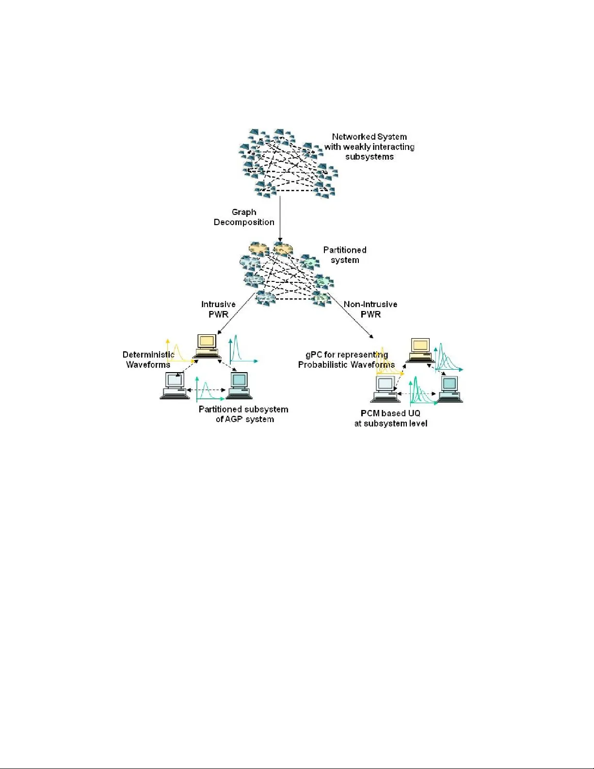
Iterativ e Metho ds for Scalable Uncertain t y Quan tification in Complex Net w orks Amit Surana, T uhin Sahai and Andrzej Banaszuk United T ec hnologies Research Cen ter, 411 Silv er Lane, East Hartford, CT 06108, USA Abstract In this pap er w e address the problem of uncertain ty management for robust design, and v erification of large dynamic netw orks whose p erformance is affected by an equally large num b er of uncertain pa- rameters. Man y such net w orks (e.g. p o wer, thermal and comm unica- tion net works) are often composed of weakly in teracting subnetw orks. W e prop ose intrusiv e and non-in trusive iterative schemes that exploit suc h weak interconnections to ov ercome dimensionalit y curse asso ci- ated with traditional uncertaint y quantification metho ds (e.g. gen- eralized P olynomial Chaos, Probabilistic Collo cation) and accelerate uncertain ty propagation in systems with large n um b er of uncertain parameters. This approach relies on integrating graph theoretic meth- o ds and w av eform relaxation with generalized P olynomial Chaos, and Probabilistic Collocation, rendering these techniques scalable. W e an- alyze con v ergence properties of this sc heme and illustrate it on several examples. 1 In tro duction The issue of managemen t of uncertain ty for robust system op eration is of in terest in a large family of complex netw ork ed systems. Examples include p o w er, thermal and comm unication net w orks which arise in sev eral instances suc h as more electric aircrafts, in tegrated building systems and sensor net- w orks. Suc h systems typically in volv e a large num ber of heterogeneous, connected comp onen ts, whose dynamics is affected by possibly an equally large n umber of uncertain parameters and disturbances. Uncertain ty Quan tification (UQ) metho ds provide means of calculating probabilit y distribution of system outputs, given probability distribution of 1 input parameters. Outputs of interest could include for example, latency in communication netw ork, pow er quality and stabilit y of p ow er netw orks, and energy usage in thermal net works. The standard UQ metho ds such as Mon te Carlo(MC) [1] either exhibit p oor con vergence rates or others suc h as Quasi Mon te Carlo (QMC) [2][3], generalized Polynomial Chaos(PC) [4] and the asso ciated Probabilistic Collo cation metho d (PCM) [5], suffer from the curse of dimensionality (in parameter space), and b ecome practically in- feasible when applied to netw ork as a whole. Improving these tec hniques to alleviate the curse of dimensionalit y is an activ e area of curren t researc h (see [6] and references therein): notable metho ds include sparse-grid collo cation metho d [7],[8] and ANO V A decomp osition [9] for sensitivit y analysis and dimensional reduction of the uncertain parametric space. How ev er, none of suc h extension exploits the underlying structure and dynamics of the net- w orked systems. In fact, man y netw orks of in terest (e.g. p o wer, thermal and comm unication netw orks), are often comp osed of weakly in teracting subsys- tems. As a result, it is plausible to simplify and accelerate the simulation, analysis and uncertain ty propagation in such systems b y suitably decom- p osing them. F or example, authors in [10, 11] used graph decomp osition to facilitate stabilit y and robustness analysis of large-scale interconnected dynamical systems. Mezic et al. [12] used graph decomp osition in con- junction with Perron F rob enius op erator theory to simplify the inv arian t measure computation and uncertain t y quan tification, for a particular class of net works. While these approaches exploit the underlying structure of the system, they do not tak e adv an tage of the weakly coupled dynamics of the subsystems. In this pap er, w e prop ose an iterative UQ approach that exploits the w eak in teractions among subsystems in a netw ork ed system to ov ercome the dimensionalit y curse asso ciated with traditional UQ metho ds. W e refer to this approac h as Probabilistic W a veform Relaxation (PWR), and prop ose b oth intrusiv e and non-intrusiv e forms of PWR. PWR relies on in tegrating graph decomp osition tec hniques and w av eform relaxation sc heme, with gPC and PCM. Graph decomp osition to identify weakly interacting subsystems, can b e realized b y spectral graph theoretic techniques [13],[14]. W av eform relaxation [15] (WR), a parallelizable iterative metho d, on the other hand, exploits this decomp osition and evolv es each subsystem forward in time in- dep enden tly but coupled with the other subsystems through their solutions from the previous iteration. In the in trusive PWR, the subsystems obtained from decomp osing the original system are used to impose a decomp osition on system obtained b y Galerkin pro jection based on the gPC expansion. F urther the weak interactions are used to discard terms which are exp ected 2 to b e insignifican t in the gPC expansion, leading to what we call an Ap- pro ximate Galerkin Pro jected (AGP) system. W e then prop ose to apply WR relaxation on the decomp osed AGP system to accelerate the UQ com- putation. In the non-in trusive form of PWR, rather than deriving the AGP system, one w orks directly with subsystems obtained from decomp osing the original system. A t eac h wa veform relaxation iteration we prop ose to apply PCM at subsystem level, and use gPC to propagate the uncertaint y among the subsystems. Since UQ metho ds are applied to relatively simpler sub- systems which typically inv olv e a few parameters, this renders a scalable non-in trusive iterative approach to UQ. W e prov e conv ergence of the PWR approac h under v ery general conditions. Note that spectral graph decom- p osition can b e done completely in a distributed fashion using a recently dev elop ed wa v e equation based clustering method [16]. Moreov er, one can further exploit timescale separation in the system to accelerate WR using an adaptiv e form of WR [17]. PWR when combined with wa v e equation based distributed clustering and adaptive WR can lead to highly scalable and computationally efficient approach to UQ in complex netw orks. This pap er is organized in six sections. In section 2 w e giv e the math- ematical preliminaries for setting up the UQ problem for net work ed dy- namical systems, and presen t an o verview of gPC and PCM tec hniques. In section 3 w e discuss graph decomp osition and w av eform relaxation metho ds, whic h form basic ingredients of PWR. Here we also describ e adaptiv e WR and wa v e equation based distributed graph decomp osition techniques. W e in tro duce the in trusiv e and non-in trusive PWR in section 4 through a simple example, and then describ e these metho ds in a more general setting. W e also prov e con vergence of PWR, and analyze the scalability of the metho d. In section 5 w e illustrate the intrusiv e and non-intrusiv e PWR on several examples. Finally , in section 6 we summarize the main results of this pap er, and presen t some future researc h directions. 2 Uncertain t y Quan tification in Net w ork ed Sys- tems Consider a nonlinear system describ ed b y a system of random differential equation ˙ x 1 = f 1 ( x , ξ 1 , t ) , . . . ˙ x n = f n ( x , ξ n , t ) , (1) 3 where, f = ( f 1 , f 2 , · · · , f n ) ∈ R n is a smo oth vector field, x = ( x 1 , x 2 , · · · , x n ) ∈ R n are state v ariables, ξ i ∈ R p i is vector of random v ariables affecting the i − th system. Let ξ = ( ξ T 1 , · · · , ξ T n ) T ∈ R p b e the p = P n i =1 p i dimensional random vector of uncertain parameters affecting the complete system. The solution to initial v alue problem x ( t 0 ) = x 0 will b e denoted by x ( t ; ξ ), where for brevity we hav e suppressed the dep endence of solution on initial time t 0 and initial condition x 0 . W e shall assume that the system (1), is Lipsc hitz || f ( x 1 , ξ , t ) − f ( x 2 , ξ , t ) || ≤ L ( ξ ) || x 1 − x 2 || , (2) where, the Lipsc hitz constant L ( ξ ) depends on the random parameter vector and || · || is a Euclidean norm. W e will assume that sup ξ ∈ R p L ( ξ ) = L < ∞ . Let us also define a set of quan tities z = ( z 1 , z 2 , · · · , z d ) = G ( x ) = ( g 1 ( x ) , · · · , g d ( x )) , (3) as observ ables or quantities of in terests. The goal is to numerically establish the effect of input uncertaint y of ξ on output observ ables z . Naturally , the solution for system (1) and the observ ables (3) are functions of same set of random v ariables ξ , i.e x = x ( t ; ξ ) , z = z ( t, ξ ) = G ( x ) . (4) In what follo ws we will adopt a probabilistic framework and mo del ξ = ( ξ 1 , ξ 2 , · · · , ξ p ) as a p − v ariate random vector with indep enden t com- p onen ts in the probabilit y space (Ω , A , P ), whose even t space is Ω and is equipp ed with σ − algebra A and probabilit y measure P . Throughout this pap er, we will assume that the parameters Σ = { ξ 1 , ξ 2 , · · · , ξ p } are mu- tually indep endent of each other. Let ρ i : Γ i → R + b e the probabilit y densit y of the random v ariable ξ i ( ω ), with Γ i = ξ i (Ω) ⊂ R b eing its im- age. Then, the joint probabilit y densit y of any random parameter s ubset Λ = { ξ i 1 , ξ i 2 , · · · , ξ i m } ⊂ Σ is given by ρ Λ ( ξ i 1 , · · · , ξ i m ) = | Λ | Y j =1 ρ i j ( ξ i j ) , ∀ ( ξ i 1 , · · · , ξ i m ) ∈ Γ Λ , (5) with a supp ort Γ Λ = | Λ | Y j =1 Γ i j ⊂ R | Λ | , (6) where, | · | denotes the cardinality of the set. Without loss of generality w e will assume that Γ i = [ − 1 1] , i = 1 , · · · , p . 4 Remark 2.1. While thr oughout the p ap er we wil l work with ODEs (1) with p ar ametric unc ertainty, the PWR fr amework develop e d in this p ap er c an b e natur al ly extende d to de al with 1) System of differ ential algebr aic e quations (D AEs), and 2) Time varying unc ertainty. Both these extensions would b e il lustr ate d thr ough examples in se ction 5. 2.1 Uncertain t y Quan tification Metho ds In this section, we describ e tw o interrelated UQ approac hes: generalized p olynomial chaos (gPC) and probabilistic collo cation metho d (PCM). The gPC is an in trusive approac h whic h requires explicit access to system equa- tions (1), while PCM is a related sampling based non-intrusiv e (and hence treats the system (1) as a blac k b o x) wa y of implementing gPC. 2.1.1 Generalized Polynomial Chaos In the finite dimensional random space Γ Σ defined in (6), the gPC expansion seeks to appro ximate a random pro cess via orthogonal p olynomials of ran- dom v ariables. Let us define one-dimensional orthogonal p olynomial space asso ciated with eac h random v ariable ξ k , k = 1 , · · · , p as W k,d k ≡ { v : Γ k → R : v ∈ span { ψ i ( ξ k ) } d k i =0 } , (7) where, { ψ i ( ξ k ) } d k i =0 denotes the orthonormal p olynomial basis from the so called Wiener-Ask ey p olynomial chaos [4]. The Ask ey sc heme of p olynomials con tains v arious classes of orthogonal p olynomials suc h that their associated w eighting functions coincide with probability density function of the under- lying random v ariables. The corresponding P -v ariate orthogonal polynomial space in Γ Σ is defined as W Σ ,P ≡ O | d |∈ P W i,d i , (8) where the tensor pro duct is o ver all possible combinations of the multi-index d = ( d 1 , d 2 , · · · , d | Σ | ) ∈ N | Σ | in set P , P = { d ∈ N | Σ | : | d | = | Σ | X i =1 d i ≤ P and d i ≤ P i } (9) and, P = ( P 1 , · · · , P | Σ | ) T ∈ N | Σ | is v ector of in tegers whic h restricts the max- im um order of expansion of i -th v ariable ξ i to be P i , and P = max i P i . Thus, 5 W Σ ,P is the space of N-v ariate orthonormal polynomials of total degree at most P with additional constraints on individual degrees of p olynomials, and its basis functions Ψ Σ ,P i ( ξ ) satisfy Z Γ Σ Ψ Σ ,P i ( ξ )Ψ Σ ,P j ( ξ ) ρ Σ ( ξ ) dξ = δ ij , (10) for all 1 ≤ i, j ≤ N Σ = dim( W Σ ,P ). Note that in standard gPC all ex- pansion orders are tak en to b e identical i.e. P 1 , = P 2 · · · = P | Σ | = P , so that dim( W Σ ,p ) = ( P + | Σ | )! P ! | Σ | ! . W e will how ever tak e adv antage of an adaptive expansion, a notion which will b e fully developed in section 4.3. The ma jor adv antage of applying the gPC is that a random differential equation can b e transformed into a system of deterministic equations. A t ypical approach is to employ a sto c hastic Galerkin pro jection, in which all the state v ariables are expanded in p olynomial c haos basis with corresp ond- ing mo dal coefficients ( a ik ( t )), as x k ( t, ξ ) ≈ x Σ ,P k ( t, ξ ) = N Σ X i =1 a ik ( t )Ψ Σ ,P i ( ξ ) , k = 1 , · · · , n, (11) where, the sum has b een truncated to a finite order. Substituting, these expansions in Eq. (1), and using the orthogonality prop erty of p olynomial c haos (10), we obtain for k = 1 , · · · , n, j = 1 , · · · , N Σ , ˙ a j k = F j k ( a , t ) , (12) a system of deterministic ODEs describing the evolution of the mo dal co ef- ficien ts, with initial conditions a j k (0) = Z Γ Σ x k (0 , ξ )Ψ Σ ,P j ( ξ ) ρ Σ ( ξ ) dξ , (13) and a = ( a 11 , · · · , a N Σ 1 , · · · , a 1 n , · · · , a N Σ n ) T , F j k ( a , t ) = Z Γ Σ f k ( x Σ ,P ( ξ , t ) , ξ k , t )Ψ Σ ,P j ( ξ ) ρ Σ ( ξ ) dξ , (14) with x Σ ,P ( t, ξ ) = ( x Σ ,P 1 ( t, ξ ) , · · · , x Σ ,P n ( t, ξ )). This system can be solved with an y numerical metho d dealing with initial-v alue problems, e.g., the Runge- Kutta metho d. Similarly , the observ able can b e expanded in gPC basis, as z k ( t, ξ ) ≈ z Σ ,P k ( t, ξ ) = N Σ X i =1 b ik ( t )Ψ Σ ,P i ( ξ ) , (15) 6 where, b j k ( t ) = Z Γ Σ z Σ ,P k ( ξ )Ψ Σ ,P j ( ξ ) ρ Σ ( ξ ) dξ (16) with k = 1 , · · · , d . Hence, once the solution to the system (12) has b een obtained, the co efficien ts b j k can b e appro ximated as b j k ≈ Z Γ Σ g k ( x Σ ,P ( t, ξ ))Ψ Σ ,P j ( ξ ) ρ Σ ( ξ ) dξ . (17) Suc h Galerkin procedures ha ve b een used extensiv ely in the literature. In man y instances Galerkin pro jection may not b e p ossible due to una v ailabilit y of direct access to the system equations (1). In many other instances such in trusive metho ds are not feasible ev en in cases when the system equations are av ailable, because of the cost of deriving and implemen ting a Galerkin system within av ailable computational tools. T o circumv en t this difficulty , probabilistic collo cation method has b een developed. 2.1.2 Probabilistic Collo cation Metho d PCM is a non-intrusiv e approac h to solving sto chastic random pro cesses with the gPC. Instead of pro jecting eac h state v ariable onto the p olynomial c haos basis, the collo cation approach ev aluates the integrals of form (16) by ev aluating in tegrand at the ro ots of the appropriate basis polynomials [5]. Giv en a 1D probability density function ρ j ( ξ j ), the PCM based on Gauss quadrature rule, approximates an integral of a function g with resp ect to densit y ρ j ( ξ j ), as follows Z 1 − 1 g ( ξ j ) ρ ( ξ j ) dξ j ≈ U l j [ g ] = m l j X k =1 w l j k g ( r l j k ) , j = 1 , · · · , p, (18) where, r l j k ∈ C l j is the set of Gauss collo cation p oin ts with asso ciated w eights w l j k , l j is the accuracy lev el of quadrature formula, and m l j is the n umber of quadrature p oints corresp onding to this accuracy level. Building on the 1D quadrature form ula, the full grid PCM leads to follo wing cubature rule, Z 1 − 1 Z 1 − 1 · · · Z 1 − 1 g ( ξ 1 , · · · , ξ p ) ρ Σ ( ξ ) dξ ≈ I ( l 1 , · · · , l p , p )[ g ] = ( U l 1 ⊗ U l 2 · · · U l p )[ g ] = m l 1 X j 1 =1 · · · m l p X j p =1 w lj g ( r lj ) , (19) 7 where, r lj = ( r l 1 j 1 , · · · , r l p j p ), with l = ( l 1 , · · · , l p ), and j = ( j 1 , · · · , j p ) and w lj = w l 1 j 1 · · · w l n j n . T o compute I ( l , p ) we need to ev aluate the function on the full collo cation grid C ( l , p ) which is giv en by tensor pro duct of 1D grids C ( l , p ) = C l 1 × · · · × C l p , (20) with a total num b er of collo cation p oin ts b eing Q = Q p j =1 m l j . In this framew ork, therefore, for any t , the appro ximations to the mo del coefficients a j k ( t ) (see Eq. (11)) and b j k ( t ) (see Eq. (15)) can b e obtained as a j k ( t ) = Z Γ Σ x Σ ,P k ( t, ξ )Ψ Σ ,P j ( ξ ) ρ Σ ( ξ ) dξ ≈ m l 1 X j 1 =1 · · · m l p X j p =1 w lj Ψ Σ ,P j ( r lj ) x k ( t, r lj ) , (21) with similar expression for b j k ( t ). Note to compute summations arising in (21), the solution x ( t, r lj ) of the system (1) is required for each collo cation p oin t r lj in the full collo cation grid C ( l , p ). Thus, simplicity of collo ca- tion framework only requires rep eated runs of deterministic solvers, without explicitly requiring the pro jection step in gPC. If w e choose the same order of collo cation p oin ts in each dimension, i.e. m l 1 = m l 2 , · · · = m l p ≡ l , the total n umber of p oin ts is Q = l p , and the computational cost increases rather steeply with the num b er of uncertain parameters p . Hence, for large systems ( n  1) with large num b er of uncertain parameters ( p  1), PCM b ecomes computationally intensiv e. As discussed in the introduction, alleviating this curse of dimensionalit y is an active area of curren t research [6]. In this pap er we prop ose a new uncertain ty quantification approach whic h exploits the underlying net work structure and dynamics to ov ercome the dimensionality curse asso ciated with PCM. The key metho dologies for accomplishing this are the graph decomp osition and wa veform relaxation, which are discussed in subsequen t sections. 3 Graph Decomp osition and W a v eform Relaxation 3.1 W a veform Relaxation In this section w e describ e the basic mathematical concept of the W av eform Relaxation (WR) metho d for iterativ ely solving the system of differential 8 equations of the form (1). F or purp oses of discussion here, w e fix the pa- rameter v alues ξ in the system (1) to fixed mean v alues. The general struc- ture of a WR algorithm for analyzing system (1) ov er a giv en time in terv al [0 , T ] consists of tw o ma jor steps: assignment p artitioning pr o c ess and the r elaxation pr o c ess [18, 15]. Assignment-p artitioning pr o c ess : Let N = { 1 , · · · , n } b e the set of state indices, and C i , i = 1 , · · · , m b e a partition of N such that N = m [ i =1 C i , C i \ C j = ∅ , ∀ i 6 = j. (22) W e shall represen t b y D : N → M ≡ { 1 , 2 , · · · , m } a map which assigns the state index to its partition index, i.e. D ( i ) = j where, j is suc h that i ∈ C j . Without loss of generalit y , w e can rewrite Eq. 1 after the assignmen t- partitioning pro cess as: ˙ y 1 = F 1 ( y 1 , d 1 ( t ) , Λ 1 , t ) . . . ˙ y m = F m ( y m , d m ( t ) , Λ m , t ) , (23) where, for each i = 1 , · · · , m , F i ≡ ( f j i 1 , · · · , f j i M i ) T , (24) y i ≡ ( x j i 1 , · · · , x j i M i ) T , (25) with initial condition y 0 i ≡ ( x 0 j i 1 , · · · , x 0 j i M i ) T , (26) and Λ i ≡ ( ξ j i 1 , · · · , ξ j i M i ) T , (27) are the sub vectors assigned to the i − th partitioned subsystem, suc h that j i k ∈ C i , k = 1 , · · · , M i = |C i | and d i ( t ) ≡ ( y T j i , · · · , y T j N i ) T , (28) is a decoupling vector, with j k ∈ M i and k = 1 , · · · , N i = |M i | . Here, M i is the set of indices of the partitions (or subsystems) with which the i − th partition (or subsystem) interacts, and is giv en by N i = M \ = ( D ( N c i )) , (29) 9 where, N c i = { j ∈ N : ∂ F i ∂ x j = 0 } and = ( · ) denotes the image of the map D . R elaxation Pr o c ess : The relaxation pro cess is an iterativ e pro cedure, with follo wing steps • Step 1: (Initialization of the relaxation process) Set I = 1 and guess an initial wa veform { y 0 i ( t ) : t ∈ [0 T ] } such that y 0 i (0) = y 0 i , i = 1 · · · , m . • Step 2: (Analyzing the decomp osed system at the I-th WR iteration) F or each i = 1 , · · · , m , set d I i ( t ) = ≡ (( y I − 1 j i ) T , · · · , ( y I − 1 j N i ) T ) T , (30) and solv e the subsystem ˙ y I i = F i ( y I i , d I i ( t ) , Λ i , t ) , (31) o ver the in terv al [0 , T s ] with initial condition y I i (0) = y 0 i , to obtain { y I ( t ) : t ∈ [0 , T s ] } . • Step 3 Set I = I + 1 and go to step 2 un til satisfactory conv ergence is ac hieved.. The general conditions for conv ergence of WR for a system of differential algebraic equations (DAEs) can be found in [18, 17]. Here, w e recall a result from [17] sp ecializing it for a system of differential equations. Prop osition 3.1. Conver genc e of WR for ODE’s (se e [18] for pr o of ): Given that the system (1) is Lipschitz (c ondition 2), then for any initial pie c ewise c ontinuous waveform { y 0 i ( t ) : t ∈ [0 , T s ] } such that y 0 i (0) = y 0 i (se e definition (26)), i = 1 · · · , m , the WR algorithm c onver ges to the solu- tion of (1) with initial c ondition x 0 . A more in tuitive analysis of error at eac h w av eform iteration is described in [17]. Let ¯ y b e the exact solution of the differen tial equation (23) and define E I to b e the error of the I -th iterate, that is E I ( t ) = y I ( t ) − ¯ y ( t ) . (32) As sho wn in [17], the error | E I | on the interv al [0 , T ] is b ounded as follo ws | E I ( t ) | ≤ C I η I T I I ! | E 0 ( t ) | , (33) 10 with C = e µT . Here C and η are related to the Lipsc hitz constan ts of the w av eform relaxation op erator [17]. It is imp ortan t to note here that the I ! in the denominator dominates the error. Thus, with enough iterations one can mak e the error fall below an y desired threshold. It is also evident from Eq. 33 that the error of standard wa v eform relaxation crucially dep ends on T . The longer the time interv al, the greater is the num b er of iterations needed to b ound the error b elo w a desired tolerance. Based on this observ ation, a no vel “adaptive” version of w av eform relaxation has b een developed in [17], whic h we refer to as adaptiv e w av eform relaxation (A WR). The idea here is to p erform wa veform relaxation in “windows” of time that are pic ked so as to reduce I in Eq. 33. Sp ecifically , one can pick small time interv als for computation when the solution to (1) changes significantly (implying E 0 ( t ) is large) and pic k large in terv als when the solution c hanges little (consequen tly E 0 ( t ) is small). The solution from one time in terv al is extrapolated to the next using a standard extrap olation formula [19] and the initial error is estimated using, ˜ E I +1 , 0 ( t ) = φ ( l ) ( x I +1 ( ξ ) , x I +1 ( ξ )) ( l + 1)! ω ( t ) , (34) where, ω ( t ) = ( t − t 0 )( t − t 1 ) . . . ( t − t l ) . (35) Here t 0 , t 1 , . . . , t l are points through which one passes the extrapolating p oly- nomial [17]. Note that, φ ( l ) = d l φ dt l is the l -th deriv ative of the wa veform relaxation op erator φ with resp ect to t (see. [19, 17]). The algorithm to compute the length of the time windows is as follows: A daptive Waveform R elaxation : T o compute the time in terv al for ∆ T I +1 , execute the following steps: 1. Set ∆ T I +1 = 2∆ T I and δ = 1 20 ∆ T I . 2. Ev aluate ˜ E I +1 , 0 ( T I + ∆ T I +1 ) using Eqn. 34 to estimate k E I +1 , 0 k and compute k ˆ E I +1 ,r k with the aid of the follo wing equation, k ˆ E I +1 ,r k =  e µ ∆ T I +1 η ∆ T I +1  r r ! k E I +1 , 0 k . (36) 3. If k ˆ E I +1 ,r k > ε and ∆ T I +1 > 1 2 ∆ T I , set ∆ T I +1 = ∆ T I +1 − δ and rep eat step 2. 11 W e define the minimal window length to b e ∆ T I +1 = 1 50 T . The abov e proce- dure gives a sequence of time interv als [0 , T 1 ], [ T 1 , T 2 ], . . . , [ T ν − 1 , T ν ], where T ν = T , on whic h WR is p erformed (as describ ed in relaxation pro cess) with an initial “guess” w av eform pro vided b y an extrap olation of the solution on the previous interv al [17]. A WR is found to accelerate sim ulations b y or- ders of magnitude ov er traditional WR [17]. In this w ork, w e prop ose to use A WR for sim ulating the set of differen tial equations that arise from in trusiv e p olynomial c haos. As men tioned b efore, the curse of dimensionalit y gives rise to a com binatorial num b er of equations [4] making A WR particularly attractiv e. While the conv ergence of WR or A WR is guaranteed irresp ectiv e of how the system is decomp osed in the assignmen t-partitioning step, the rate of con vergence dep ends on the decomp osition [17]. F or a given nonlinear sys- tem, determining a decomp osition that leads to an optimal rate of A WR con vergence is an NP-complete problem [17]. Ideally , to minimize the num- b er of iterations required for conv ergence, one w ould lik e to place strongly in teracting equations/v ariables on a single pro cessor, with w eak interactions b et w een the v ariables or equations on different pro cessors. W e sho w in [17], that sp ectral clustering [13] along with horizontal v ertical decomp osition [12] is a go od heuristic for decomp osing systems for fast conv ergence in WR and A WR. F or this task, we no w discuss a nov el decentralized spectral clustering approac h [16] that when coupled with A WR [17] pro vides a p o werful tool for sim ulating large dynamical systems. 3.2 Graph Decomp osition The problem of partitioning the system of equations (1) in to subsystems based on how they interact or are coupled to eac h other, can b e form ulated as a graph decomp osition problem. Giv en the set of states x 1 , · · · , x n and some notion of dep endence w ij ≥ 0 , i = 1 , · · · , n, j = 1 , · · · , n b etw een pairs of states, an undirected graph G = ( V , E ) can b e constructed. The v ertex set V = { 1 , . . . , n } in this graph represen t the states x i , and the edge set is E ⊆ V × V , where a weigh t ¯ w ij ≥ 0 is asso ciated with each edge ( i, j ) ∈ E , and W = [ ¯ w ij ] is the n × n weigh ted adjacency matrix of G . In order to quan tify coupling strength ¯ w ij b et w een no des or states, we prop ose to use ¯ w ij = 1 2 [ | J ij | + | J j i | ] , (37) 12 where, J = [ 1 T s R t 0 + T s t 0 J ij ( x ( t ; ξ m ) , ξ m , t ) dt ], is time av erage of the Jacobian, J ( x , ξ , t ) =  ∂ f i ( x ( t ; ξ ) , ξ , t ) ∂ x j  , (38) computed along the solution x ( t ; ξ ) of the system (1) for nominal v alues of parameters ξ m . Use of system Jacobian for horizontal v ertical graph decomp osition can also b e found in [12]. W e will now discuss, sp ectral clustering (see [13] a p opular graph de- comp osition/clustering approach that allo ws one to partition a undirected graph giv en its adjacency matrix W . In this m ethod first a (normalized) graph Laplacian is constructed as follows [14, 20, 21], L ij =      1 if i = j − ¯ w ij / P N ` =1 ¯ w i` if ( i, j ) ∈ E 0 otherwise , (39) or equiv alen tly as, L = I − D − 1 W where D is the diagonal matrix with the ro w sums of W . The clustering assignmen t/decomp osition is then obtained b y computing the eigenv ectors/eigenv alues of L . In particular, one uses the signs of the comp onen ts of the second and higher eigen vectors to partition the nodes in the graph into clusters [13]. T raditionally , one can use standard matrix algorithms for eigen vectors/eigen v alues computation [22]. How ever, as the size of the dynamical system or net work (and th us corresp onding adjacency matrix) increases, the execution of these standard algorithms b e- comes infeasible on monolithic computing devices. T o address this issue, distributed eigenv alue/eigen vector computation metho ds hav e b een devel- op ed, see for example [23]. In [16], a w av e equation based distributed algorithm to partition large graphs has been dev elop ed whic h computes the partitions without construct- ing the entire adjacency matrix W of the graph [13]. In this metho d one “hears” clusters in the graph b y computing the frequencies (using F ast F ourier T ransform (FFT) lo cally at each no de) at which the graph “res- onates”. In particular, one can sho w that these “resonant frequencies” are related to the eigenv alues of the graph Laplacian L (39) and the co efficien ts of FFT expansion are the comp onen ts of the eigen vectors. Infact, the al- gorithm is pro v ably equiv alen t to the standard sp ectral clustering [13], for details see [16]. The steps of the w av e equation based clustering algorithm are as follows. One starts b y writing the lo cal up date equation at no de i based on the 13 discretized w av e equation, u i ( t ) = 2 u i ( t − 1) − u i ( t − 2) − c 2 X j ∈N i L ij u j ( t − 1) (40) where u i ( t ) is the v alue of u at no de i at time t and L ij are the lo cal en tries of the graph Laplacian. A t eac h no de i , u i (0) = u i ( − 1) is set to a random n umber on the in terv al [0 , 1]. One then updates the v alue of u i using Eqn. (40) until t = T max (for a discussion on how to pic k T max see [16]). Note that, u i ( t ) is a scalar quantit y and one only needs nearest neighbor information in Eqn. (40) to compute it. One then performs a lo cal FFT on [ u i (1) , . . . . . . , u i ( T max )] and then assigns the co efficien ts of the peaks of the FFT to v ij . Here the frequency of the j -th p eak is related to λ j , the j -th eigen v alue of the graph Laplacian L , and v ij is the i -th comp onen t of the j -th eigenv ector. In [16], it has b een shown that for the wa ve sp eed c < √ 2 in Eqn. (40) ab o ve wa ve equation based iterative algorithm is stable and conv erges. Moreo ver, the algorithm con v erges in O ( √ τ ) steps, where τ is the mixing time of the Marko v Chain [16] asso ciated with the graph G . The comp eting state-of-the-art algorithm [23] con verges in O ( τ (log( n ) 2 ). F or large graphs or datasets, O ( √ τ ) conv ergence is sho wn to provide orders of magnitude impro vemen t ov er algorithms that con verge in O ( τ (log( n ) 2 ). F or detailed analysis and deriv ations related to the algorithm, we refer the reader to [16]. 4 Scalable Uncertain t y Quan tification Approac h In this section w e discuss how gPC and PCM can b e in tegrated with WR sc heme extending it to a probabilistic setting. As mentioned earlier w e re- fer to this iterative UQ approach as PWR. Figure 1 shows the schematic of PWR framew ork. In the intrusiv e PWR, the subsystems obtained from decomp osing the original system are used to imp ose a decomp osition on sys- tem obtained by Galerkin pro jection based on the gPC expansion. F urther the w eak interactions are used to discard terms which are exp ected to be insignifican t in the gPC expansion, leading to what we call an Approximate Galerkin Pro jected (AGP) system. W e then propose to apply standard or adaptiv e WR on the decomp osed A GP system to accelerate the UQ com- putation. In the non-in trusive form of PWR, rather than deriving the AGP system, one w orks directly with subsystems obtained from decomp osing the original system. A t eac h wa veform relaxation iteration we prop ose to apply PCM at subsystem level, and use gPC to propagate the uncertaint y among 14 Figure 1: Schematic of in trusive (left) and non-in trusive (right) PWR. the subsystems. Note that unlik e in trusive PWR (where deterministic de- coupling vectors or deterministic w av eforms are exc hanged), in non-in trusive PWR, stochastic decoupling vector or probabilistic w av eforms represen ted in gPC basis are exchanged b etw een subsystems at eac h iteration. W e first describ e the k ey tec hnical ideas b ehind intrusiv e and non-intrusiv e PWR though an illustration on a simple example in section 4.1. These no- tions are fully generalized later in sections 4.2-4.4. W e also prov e the con- v ergence of PWR approac h (in section 4.5), and in section 4.6 discuss the computational gain it offers ov er standard application of gPC and PCM. 15 4.1 Main Ideas of PWR W e illustrate the prop osed PWR framework through an example of para- metric uncertain ty in a simple system (1). Consider the follo wing coupled oscillator system: ˙ x 1 = f 1 ( x 1 , x 2 , ω 1 , t ) = ω 1 + K 12 sin( x 1 − x 2 ) , ˙ x 2 = f 2 ( x 1 , x 2 , x 3 , ω 2 , t ) = ω 2 + K 21 sin( x 1 − x 2 ) + K 23 sin( x 3 − x 2 ) , (41) ˙ x 3 = f 3 ( x 2 , x 3 , ω 3 , t ) = ω 1 + K 32 sin( x 2 − x 3 ) Here, ω i is the uncertain angular frequency of the i th ( i = 1 , 2 , 3) oscilla- tor. W e assume that parameters ω i are mutually indep enden t, each ha ving probabilit y density ρ i = ρ i ( ω i ). The coupling matrix K is K =   0 K 12 0 K 21 0 K 23 0 0 K 32   (42) is assumed deterministic with K ij = O (  ) ,   1, so that the three oscillators in (1) w eakly in teract with eac h other, i.e. the subsystem 2 weakly affects subsystem 1 and 3, and vice v ersa. 4.1.1 Approximate Galerkin pro jection for the simple example In standard gPC, states x i are expanded in a p olynomial chaos basis as x Σ ,P i ( t, ω ) = N Σ X j =1 a j i ( t )Ψ Σ ,P j ( ω ) , i = 1 , 2 , 3 (43) where, Ψ Σ ,P j ∈ W Σ ,P , the P v ariate p olynomial chaos space formed ov er Σ = { ω 1 , ω 2 , ω 3 } and P = ( P 1 , P 2 , P 3 ) determines the expansion order(see section 2.1.1 for details). Note that in this expansion (43), the system states are expanded in terms of all the random v ariables ω affecting the entire system. F rom the structure of system (1) it is clear that the 1 st subsystem is directly affected by the parameter ω 1 and indirectly b y parameter ω 2 through the the state x 2 . W e neglect second order effect of ω 3 on x 1 . A similar statement holds true for subsystem 3, while subsystem 2 will b e w eakly influenced by ω 1 and ω 3 through states x 1 and x 3 , resp ectively . This 16 structure can b e used to simplify the Galerkin pro jection as follows. F or x 1 w e consider the gPC expansion o ver Σ 1 = Λ 1 S Λ c 1 , x Σ 1 ,P 1 1 ( t, ω 1 , ω 2 ) = N Σ 1 X j =1 a j 1 ( t )Ψ Σ 1 ,P 1 j ( ω 1 , ω 2 ) , (44) where, Λ 1 = { ω 1 } , Λ c 1 = { ω 2 } (45) and P 1 = ( P 11 , P 12 ). Note that since ω 2 w eakly affects x 1 , the order of expansion P 12 can b e chosen to b e smaller compared to P 11 . Similarly , one can consider simplification for x Σ 3 ,P 3 3 ( t, ω 1 , ω 3 ). F or x 2 follo wing similar steps, w e define Λ 2 = { ω 2 } , Λ c 2 = { ω 1 , ω 3 } (46) and P 2 = ( P 21 , P 22 , P 23 ). By similar argument, one will choose P 21 , P 23 m uch smaller than P 22 . W e also in tro duce the follo wing tw o pro jections asso ciated with the state x 2 : P 2 ,i ( x Σ 2 ,P 2 2 ) = N Σ i X j =1 D x Σ 2 ,P 2 2 , Ψ Σ i ,P 2 j E Ψ Σ i ,P i j . (47) where i = 1 , 3 and h· , ·i is the appropriate inner pro duct on W Σ ,P (see section 4.3 for details). With these expansions, and using standard Galerkin pro jection we obtain the follo wing system of deterministic equations ˙ a = F ( a , t ) , (48) with appropriate initial conditions, where F j 1 ( a ) = Z Γ Σ f 1 ( x Σ 1 ,P 1 1 , P 2 , 1 ( x Σ 2 ,P 1 2 ) , ω 1 , t )Ψ Σ 1 ,P 1 j ( ω ) ρ ( ω ) dω , , F j 2 ( a ) = Z Γ Σ f 2 ( x Σ 1 ,P 1 1 , x Σ 2 ,P 2 2 , x Σ 3 ,P 3 3 , ω 2 , t )Ψ Σ 2 ,P 2 j ( ω ) ρ ( ω ) dω , F j 3 ( a ) = Z Γ Σ f 3 ( P 2 , 3 ( x Σ 2 ,P 2 2 ) , x Σ 1 ,P 1 1 , ω 3 , t )Ψ Σ 3 ,P 3 j ( ω ) ρ ( ω ) dω , and a = ( a 1 , a 2 , a 3 ) T , with a i = ( a i 1 , · · · , a iN Σ i ) and F = ( F 1 , F 2 , F 3 ) T with F i = ( F i 1 , · · · , F 1 N Λ i ). W e will refer to (48) as an approximate Galerkin pro jected (AGP) system. The notion of AGP in more general setting is describ ed in section 4.3. 17 4.1.2 Intrusiv e PWR illustrated on the simple example In intrusiv e PWR, after p erforming the A GP explicitly , the system (48) is decomp osed as ˙ a ij = F j i ( a i , d i , t ) , (49) where d 1 = P 2 , 1 ( a 2 ), d 2 = ( a 1 , a 3 ) and d 3 = P 2 , 1 ( a 2 ) are the decoupling v ectors (here we o verloaded notation for P 2 ,i ( a 2 ) to imply the coefficients in expansion (47)). Note that the decomp osition of system (48) is based on the decomp osition of the original system (41). Adaptive or standard WR describ ed in section 3.1, can then be applied to solv e the decomp osed system (49), iteratively . Since, the the system (49) is deterministic, deterministic w av eforms or deterministic decoupling vectors d i , i = 1 , 2 , 3 are exc hanged in eac h WR iteration (see Figure 1 for an illustration). 4.1.3 Non-Intrusiv e PWR illustrated on the simple example In the non-in trusive form of PWR, rather than deriving the A GP , one w orks directly with subsystems obtained from decomp osing the original system. The main idea here is to apply PCM at subsystem level at each PWR iter- ation, use gPC to represent the probabilistic wa veforms and iterate among subsystems using these w av eforms. Recall that in standard PCM approach (2.1.2), the co efficien ts a i m ( t ) are obtained by calculating integral a mi ( t ) = Z x Λ i ,P i i ( t, ω )Ψ Λ i ,P i m ( ω ) ρ Λ i ( ω ) dω (50) The in tegral abov e is t ypically calculated b y using a quadrature form ula and rep eatedly solving the i th subsystem ov er an appropriate collo cation grid C i (Σ i ) = C i (Λ i ) × C i (Λ c i ), where, C i (Λ i ) is the collo cation grid corresp onding to parameters Λ i (and let l s b e the num b er of grid p oints for eac h random parameter in Λ i ), C i (Λ c i ) is the collo cation grid corresp onding to parameters Λ c i (and let l c b e the n umber of grid p oin ts for eac h random parameter in Λ c i ). Since, the b eha vior of i th subsystem is weakly affected by the parameters Λ c i , we can take a sparser grid in Λ c i dimension, i.e. l c < l s , as w e to ok lo wer order expansion for these random v ariables in section 4.1.1. Belo w we outline k ey steps in non in trusive PWR: • Step 1: (Initialization of the relaxation pro cess with no coupling ef- fect): Set I = 1, guess an initial wa veform x 0 i ( t ) consistent with initial condition. Set d 1 1 = x 0 2 , d 1 2 = ( x 0 1 , x 0 3 ) , d 1 3 = x 0 2 , and solve ˙ x 1 i = f i ( x 1 i , d 1 i ( t ) , ω i , t ) , (51) 18 with an initial condition x 1 i (0) = x 0 i (0) on a collo cation grid C i (Λ i ). Determine the gPC expansion x Λ i ,P i , 1 i ( t, · ) b y computing the expansion co efficien ts from the quadrature formula (50). • Step 2: (Initialization of the relaxation pro cess, incorp orating first lev el of coupling effect): Set I = 2 and let d 2 1 = x Λ 2 ,P 2 , 1 2 , d 2 2 = ( x Λ 1 ,P 1 , 1 1 , x Λ 3 ,P 3 , 1 3 ) , d 2 3 = x Λ 2 ,P 2 , 1 2 b e the sto chastic de c oupling ve ctors . Solv e ˙ x 2 i = f i ( x 2 i , d 2 i ( t, · ) , ω i , t ) , (52) o ver a collo cation grid C i (Σ i ) to obtain x Σ i ,P i , 2 i ( t, · ). F rom now on w e shall denote the solution of the i th subsystem at I th iteration b y x Σ i ,P i ,I i . • Step 3 (Analyzing the decomp osed system at the I-th iteration): Set the decoupling v ectors, d I 1 = P 2 , 1 ( x Σ 2 ,P 2 ,I − 1 2 ) , d I 2 = ( x Σ 1 ,I − 1 1 , x Σ 3 ,P 3 ,I − 1 3 ), d I 3 = P 2 , 3 ( x Σ 2 ,P 2 ,I − 1 2 ) and solve ˙ x I i = f i ( x I i , d I i ( t, · ) , ω i , t ) , (53) o ver a collo cation grid C i (Σ i ) and obtain the expansion x Σ i ,P i ,I i ( t, · ). • Step 4 (Iteration) Set I = I + 1 and go to step 5 un til satisfactory con vergence has b een achiev ed. Note that in ab o ve non-in trusive PWR, the decoupling v ectors are stochastic and so at each iteration pr ob abilistic waveforms are exchanged betw een sub- systems ((see Figure 1 for an illustration). W e next generalize the intrusiv e and non-in trusive PWR in tro duced ab o v e, in the forthcoming sections. 4.2 Decomp osition of Galerkin Pro jected System W e begin b y revisiting the complete Galerkin system (12). T o apply WR, recall that the first step is the assignmen t-partitioning (see section 3.1). There are tw o p ossible approaches for partitioning the complete Galerkin system. One can first split the original dynamical system (1), and then use this decomp osition to partition the complete Galerkin pro jection (12) by assigning the mo del co efficien ts in (11) for each state to the cluster to which state is assigned to while decomp osing system (1). As previously explained in section 3.2, the partitioning is p erformed by representing the dynamical system (1) as a graph with the symmetrized time av eraged Jacobian (37) as the w eighted adjacency matrix. One can then apply the w av e equation based decen tralized clustering algorithm outlined in section 3.2. 19 Alternativ ely , one can p erform this decomp osition directly on the com- plete Galerkin pro jection (12). Let the symmetrized time a veraged Jacobian for the resulting system (12) b e, ˜ w ij = 1 2 [ | ˜ J ij | + | ˜ J j i | ] , (54) where, ˜ J = [ 1 T s R t 0 + T s t 0 J 0 ij ( a ( t ) , t ) dt ], is time av erage of the Jacobian, J 0 ( a , t ) =  ∂ F ik ( a ( t )) ∂ a ik  , (55) computed along the solution a ( t ) of the system (12). This giv es, J 0 ( a , t ) = Z Γ Σ ∂ f k ( x Σ ,P ( ξ , t ) , ξ k , t ) ∂ a j k Ψ Σ ,P i ( ξ ) w Σ ( ξ ) dξ . (56) T aylor expanding f k ( x ( ξ , t ) , ξ k , t ) lo cally , giv es, J 0 ( a , t ) ≈ J ( a , t ) . (57) Th us, one exp ects to get similar results by p erforming clustering on the original system (in (1)) to that obtained based on complete Galerkin sys- tem (12). Since the dimensionalit y of system (1) is m uch lo w er than that of system (12), the first decomp osition is less computationally challenging than the latter. In this work, w e will use the original system to determine the decomp osition and use that to imp ose the partition of the Galerkin pro- jection. Given the decomp osition of system (12), one can use the WR or its adaptiv e form to simulate the system in a parallel fashion. How ever, b efore doing this one can further exploit the weak interaction b et ween subsystems to reduce the dimensionality of the complete Galerkin system, as describ ed in section 4.1.1. W e next describ e this approximate Galerkin pro jection in a more general setting. 4.3 Appro ximate Galerkin Pro jection and Intrusiv e Proba- bilistic W a v eform Relaxation Recall that in the gPC expansion (11), all the system states are expanded in terms of random v ariables affecting the entire system. Ho wev er, the i − th subsystem in the decomp osition (see Eq. (23)) is directly affected b y the parameters Λ i (see definition (27)) and indirectly b y other parameters through the decoupling vector (see definition (28)). W e shall denote b y Λ c i = [ j ∈N i Λ j , (58) 20 the set of parameters which indirectly affect the i − th subsystem through the immediate neighbor interactions and by Σ i = Λ i ∪ Λ c i , (59) the set of parameters that directly and indirectly (through nearest neigh- b or interaction) affect the i − th subsystem. Under the h yp othesis that the i − th subsystem is dynamically w eakly coupled with its nearest neighbors, uncertain ty in parameters Λ i c will weakly influence the states in i − th sub- system through the decoupling vector, while the uncertaint y in parameters Σ \ Σ i can b e neglected. T o capture this effect, consider a P -v ariate space (analogous to the P -v ariate space in tro duced in the section 2.1.1) W Λ ,P ≡ O | d |∈ P W k i ,d k i , (60) formed ov er any random parameter subset Λ = { ξ i 1 , ξ i 2 , · · · , ξ i n } ⊂ Σ. W e shall denote the basis elemen ts of W Λ ,P b y Ψ Λ ,P i , i = 1 , · · · , N Λ , where N Λ = dim( W Λ ,P ). Note that for an y Λ 1 ⊂ Λ 2 ⊂ Σ, W ∅ ⊂ W Λ 1 ,P 1 ⊂ W Λ 2 ,P 2 ⊂ W Σ ,P , (61) where, W ∅ = { 0 } is the P − v ariate space corresponding to the empt y set. Also, recall that P 1 , P 2 are v ectors whic h con trol the expansion order in gPC expansion. The inner pro duct on W Σ ,P induces an inner pro duct on W Λ ,P as follo ws < X 1 ( ξ ) , X 2 ( ξ ) > Λ = Z Γ Λ X 1 ( ξ ) X 2 ( ξ ) ρ Λ ( ξ ) dξ , (62) for an y X 1 ( ξ ) , X 2 ( ξ ) ∈ W Λ ,P . Using this inner pro duct, we introduce a pro jection op erator P r Λ 2 Λ 1 : W Λ 2 ,P 2 → W Λ 1 ,P 1 , (63) suc h that for an y X ( ξ ) ∈ W Λ 2 ,P 2 P r Λ 2 ,P 2 Λ 1 ,P 1 ( X )( ξ ) = N Λ 1 X i =1 < X , Ψ Λ 1 ,P 1 S i > Λ Ψ Λ 1 ,P 1 i ( ξ ) . (64) With resp ect to the given decomp osition D imp osed on the system (see section 3.1), we define a pro jection op erator P i,j indexed b y subsystem i and state x j P i,j ≡        P r Σ ,P Σ i ,P i , if D ( j ) = i, P r Σ ,P Λ D ( j ) S (Λ c D ( j ) T Λ i ) ,P i if D ( j ) 6 = i, N i T N D ( j ) 6 = ∅ , P r Σ ,P ∅ if D ( j ) 6 = i, N i T N D ( j ) = ∅ . 21 Remark 4.1. F or any subsystem i , sinc e the p ar ameters Λ c i we akly affe ct it, we c an adaptively sele ct c omp onent of ve ctor P i = ( P i 1 , · · · , P i, | Σ i | ) so that a lower or der exp ansion is use d in c omp onents c orr esp onding to r andom variables in Λ c i . F or any subsystem i and a vector x Σ ,P ( ξ , t ) = ( x Σ ,P k 1 ( ξ , t ) , · · · , x Σ ,P k n ( ξ , t )) (where x Σ ,P i ( ξ , t ) is standard gPC expansion (11)), we asso ciate a vector v alued pro jection op erator as follows P i ( x Σ ,P ) = ( P i,k 1 ( x Σ ,P k 1 ) , · · · , P i,k n ( x Σ ,P k n )) . (65) In terms of these op erators, for an y state x k , an approximate Galerkin pro- jected equation is defined as, d dt P i,k [ x Σ ,P k ( ξ , t )] = f k ( P i ( x Σ ,P ( ξ , t )) , ξ k , t ) , (66) where, i = D ( k ) is the index of the subsystem to which the state k b elongs. More, precisely the ab o ve system can b e expressed as: ˙ a i j k = F i j k ( a , t ) , (67) where, a = ( a D (1) 11 , · · · , a D (1) N Σ D (1) , 1 , · · · , a D ( n ) 1 n , · · · , a D ( n ) N Σ D ( n ) ,n ) T F i j k = Z Γ Σ i f k ( P i ( x Σ ,P ( ξ , t )) , ξ k , t )Ψ Σ i ,P i j ( ξ ) ρ Σ i ( ξ ) dξ , (68) and, j = 1 , · · · , N Σ i , k = 1 , · · · , n with i = D ( k ). Let F = ( F D (1) 11 , · · · , F D (1) N Σ D (1) , 1 , · · · , F D ( n ) 1 n , · · · , F D ( n ) N Σ D ( n ) ,n ) T , then the system (67) can b e compactly written as ˙ a = F ( a , t ) , (69) with appropriate initial condition (see expression 13) and will b e referred to as the approximate Galerkin pro jected (AGP). Using this generalization of AGP system, it is straightforw ard to generalize the intrusiv e PWR intro- duced in section 4.1.2. 22 4.3.1 Intrusiv e PWR Algorithm In the intrusiv e PWR, one applies the WR to A GP system. As p er discussion in s ection 4.2, the decomp osition D on the original system (1) is used to imp oses a decomp osition on the system (69) leading to ˙ a i = F i ( a i , d i , t ) , (70) for i = 1 , · · · , m , where a i = ( a i 1 k 1 , · · · , a i N Σ i ,k 1 , · · · , a i 1 k |C i | , · · · , a i N Σ i ,k |C i | ) T , (71) F i = ( F i 1 k 1 , · · · , F i N Σ i ,k 1 , · · · , F i 1 k |C i | , · · · , F i N Σ i ,k |C i | ) T , (72) k i ∈ C i , and d i = ( a T j i , · · · , a T j N i ) T is the decoupling v ector (recall notation from section 3.1). One then follows the procedure for w av eform relaxation or its adaptiv e version, as described in section 3.1. Adaptiv e WR can lead to a significant increase in con vergence of WR as demonstrated in [17], and w ould b e illustrated later in the section 5. As discussed in section 2.1.1, the pro jection step (66) can b e very tedious and in some cases not possible. Hence, applying w a veform relaxation directly to the system (70) may not b e practical in many instances. In the next section, w e describ e an alternativ e non-in trusive approach using probabilistic collo cation, which do es not require the pro jection step (66) explicitly . 4.4 Non-In trusiv e Probabilistic W a v eform Relaxation In terms of the pro jection op erator (65), we can rewrite each subsystem in (23) as ˙ y i = F i ( y i , P i ( d i ( t, · )) , Λ i , t ) , (73) where, d i ( t, · ) is the sto chastic de c oupling ve ctor or pr ob abilistic waveform , d i ( t, · ) = (( y Σ j 1 ,P j 1 j i ) T , · · · , ( y Σ j N i ,P j N i j N i ) T ) T . (74) where, w e ha ve explicitly indicated the dep endence on the parameters ( see definition (28)). Here for any i = 1 , · · · , m , y Σ i ,P i = ( x Σ i ,P i j i 1 , · · · , x Σ i ,P i j i M i ) T , with x Σ i ,P i j i k ( ξ , t ) = N Σ i X m =1 a mj i k ( t )Ψ Σ i ,P i m ( ξ ) = P i,j i k ( x Σ ,P j i k ) , (75) 23 By definition the co efficien ts a mj i k ( t ) in ab o ve expansion satisfy the system (67). These co efficien ts can b e obtained by using the quadrature formula (21), by rep eatedly solving the system (73) ov er an appropriate collo cation grid C ( l , n i ) C ( l , n i + n c i ) = C ( o , n i ) × C ( m , n c i ) , (76) where, l = ( o , m ), C ( o , n i ) = C 1 o 1 × · · · × C 1 o n i , is the collo cation grid corresp onding to parameters Λ i , with n i = | Λ i | , o = ( o 1 , · · · , o n i ), and C ( m , n c i ) = C 1 m 1 × · · · × C 1 m n c i , is the collocation grid corresp onding to pa- rameters Λ c i , with n c i = | Λ c i | and m = ( m 1 , · · · , m n c i ). F or simplicit y we tak e o 1 = · · · = o n i = l s and m 1 = · · · = m n c i = l c for i = 1 · · · , m . Since, the b eha vior of i − th subsystem is w eakly affected b y the parameters Λ c i through the decoupling vector, then consistent with remark (4.1) we can take l c < l s , (77) leading to an adaptiv e collocation grid for each subsystem. With this, w e are ready to generalize the non-in trusive PWR approac h in tro duced in section 4.1.3. 4.4.1 Non-Intrusiv e PWR Algorithm • Step 1: Apply graph decomp osition (see section 3 for details) to iden- tify w eakly interacting subsystems in the system (1). • Step 2 (Assignment-partitioning process): Partition (1) into m sub- systems (obtained in Step I) leading to system of equations given b y (23). Obtain, Λ i , Λ c i and Σ i for each subsystem, i = 1 , · · · , m . Cho ose the parameters l si , l ci , P i . • Step 3: (Initialization of the relaxation pro cess with no coupling ef- fect): Set I = 1 and , guess an initial w av eform { y 0 i ( t ) : t ∈ [0 , T s ] } for eac h i = 1 , · · · , m consisten t with initial condition (see Step 1 in relaxation pro cess described in section 3.1). Set d 1 i ( t ) = ( y j 1 ( t ) , · · · , y j N i ( t )) , (78) i = 1 , · · · , m , and solve for { y Λ i ,P i , 1 i ( t ) , t ∈ [0 , T s ] } using ˙ y 1 i = F i ( y 1 i , d 1 i ( t ) , Λ i , t ) , (79) with an initial condition y 1 i (0) = y 0 i (0) on a collo cation grid C ( o , n i ). Determine the gPC expansion y Λ i ,P i , 1 i ( t, · ) ov er P − v ariate p olynomial 24 space W Λ i ,P i b y computing the expansion coefficients from the quadra- ture form ula (21). • Step 4: (Initialization of the relaxation pro cess, incorp orating first lev el of coupling effect): Set I = 2 and for eac h i = 1 , · · · , m , set d 2 i ( t, · ) = ( y Λ j 1 ,P j 1 , 1 j 1 ( t, · ) , · · · , y Λ j N i ,P j N i , 1 j N i ( t, · )) , (80) and solv e for { y 2 i ( t ) , t ∈ [0 , T s ] } from ˙ y 2 i = F i ( y 2 i , d 2 i ( t, · ) , Λ i , t ) , (81) with an initial condition y 2 i (0) = y 0 i (0), ov er a collo cation grid C ( l , n i + n c i ). Obtain the expansion y Σ i ,P i , 2 i ( t, · ) using (75). F rom no w on w e shall denote the solution vector of the i − th subsystem at I − th itera- tion b y y Σ i ,P i ,I i . • Step 5 (Analyzing the decomp osed system at the I-th iteration): F or eac h i = 1 , · · · , m , set d I i = ( y Σ j 1 P j 1 , ( I − 1) j 1 , · · · , y Σ j N i ,P j N i , ( I − 1) j N i ) , (82) and solv e for { y I ( t ) : t ∈ [0 , T s ] } from ˙ y I i = F i ( y I i , P i ( d I i ( t, · )) , Λ i , t ) , (83) with initial condition y I i (0) = y 0 i (0) o ver a collo cation grid C ( l , n i + n c i ). Obtain the expansion y Σ i ,P i ,I i ( t, · ) using the expansions (75). • Step 6 (Iteration) Set I = I + 1 and go to step 5 un til satisfactory con vergence has b een achiev ed. 4.5 Con v ergence of PWR Belo w w e pro ve that the iterative PWR approac h con v erges. The pro of is based on sho wing that the A GP system is Lipsc hitz if the orginal systems is Lipschitz (see condition 2), and then inv oking standard WR conv ergence result (3.1). Prop osition 4.2. Conver genc e of PWR: The intrusive and non-intrusive PWR algorithms describ e d in se ctions 4.3.1 and 4.4.1, r esp e ctively c onver ge. 25 Pr o of: W e pro ve the result for in trusive PWR. By construction, since non-in trusive PWR algorithm solv es the A GP system (69) in a differen t w ay , the con v ergence result holds for non-intrusiv e PWR as w ell. Consider the A GP system(69) and let a 1 = ( a 1 D (1) 11 , · · · , a 1 D (1) N Σ D (1) , 1 , · · · , a 1 D ( n ) 1 n , · · · , a 1 D ( n ) N Σ D ( n ) ,n ) T , (84) and a 2 = ( a 2 D (1) 11 , · · · , a 2 D (1) N Σ D (1) , 1 , · · · , a 2 D ( n ) 1 n , · · · , a 2 D ( n ) N Σ D ( n ) ,n ) T . (85) Let for a given k = 1 , · · · , n , i = D ( k ), then P i,k ( x l, Σ ,P k ( t, ξ )) = N Σ i X j =1 a li j k ( t )Ψ Σ i ,P j ( ξ ) , (86) and P i ( x l, Σ ,P ) = ( P i, 1 ( x l, Σ ,P 1 ) , · · · , P i,n ( x l, Σ ,P n )), for l = 1 , 2 and for sim- plifying notation w e hav e dropp ed subscripts on P v ectors. Then for eac h k = 1 , · · · , n , i = D ( k ), j = 1 , · · · , N Σ i , || F i j k ( a 2 ) − F i j k ( a 1 ) || = | Z Γ Σ ( f k ( P i ( x Σ ,P, 2 ) , ξ , t ) − f k ( P i ( x Σ ,P, 1 ) , ξ , t )) × Ψ Σ i ,P j ( ξ ) w Σ ( ξ ) dξ | ≤ Z Γ Σ L ( ξ )( n X m =1 N Σ D ( m ) X p =1 | ( a l, D ( m ) pm − a 2 , D ( m ) pm )Ψ Σ D ( m ) ,P p | ) ×| Ψ Σ i ,P j ( ξ ) | w Σ ( ξ ) dξ ≤ n X m =1 N Σ D ( m ) X p =1 L i D ( m ) pj | ( a 1 , D ( m ) pm − a 2 , D ( m ) pm ) | (87) where, L iq pj = Z Γ Σ L ( ξ ) | Ψ Σ q ,P p ( ξ ) || Ψ Σ i ,P j ( ξ ) | w Σ ( ξ ) dξ . (88) F or a given i = 1 , · · · , n and j = 1 · · · , N Σ D ( i ) , let L g ij = [ L D ( i ) D (1) j 1 · · · L D ( i ) D (1) j N Σ D (1) · · · L D ( i ) D ( n ) j 1 · · · L D ( i ) D ( n ) j N Σ D ( n ) ] , 26 and define L g i =     L g i 1 . . . L g iN Σ D ( i )     , L g =    L g 1 . . . L g n    , (89) then, || F ( a 2 ) − F ( a 1 ) || ≤ L || a 2 − a 1 || , (90) where, L = || L g || is a matrix norm of L g . Hence, the system (69) is Liptc hitz. Th us, giv en the original system (1) is Lipschitz (condition (2)), the approx- imate system (69) is also Lipschitz as sho wn ab o ve (90). Hence, by prop o- sition 3.1 (adaptation of Theorem 5.3 in ([18])), we conclude that PWR con verges. The question of how the decomp osition of the system and the choice of the PWR algorithm parameters P , l s , l c influence: 1) the rate of conv ergence of PWR, and 2) the appro ximation error (due to the truncation in tro duced in the AGP system (69), the use of adaptive collo cation grid i.e. condition 77 and computation of the modal co efficien ts by the quadrature form ula), needs to b e further in vestigated. 4.6 Scalabilit y of PWR The scalability of non-intrusiv e PWR relative to full grid PCM is shown in Figure 10, where the ratio R F / R I indicates the computation gain o ver standard full grid approac h applied to the system (1) as a whole. Here R F = l p is the num b er of deterministic runs of the complete system (1), whic h comprises of m subsystems eac h with p i , i = 1 , · · · , m uncertain pa- rameters, such that p = P m i =1 p i and l denotes the level of full grid. Similarly , R I = 1 + P m i =1 l p i s + I max ( P m i =1 l p i s N j 6 = i l p j c ) is the total computational effort with PWR algorithm, where I max is the n um b er of PWR iterations. Clearly , the adv an tage of PWR b ecomes eviden t as the n umber of subsystems m and parameters in the net work increases. Moreo ver PWR is inheren tly paralleliz- able. 5 Example Problems In this section w e illustrate in trusiv e and non-intrusiv e PWR through sev eral examples of linear and nonlinear netw orked systems with increasing num b er of uncertain parameters. While most examples are of ODE’s, w e also giv e 27 Figure 2: Scalabilit y of PWR algorithm, when implemented with full grid collo cation as the subsystem level UQ metho d, with p i = 5 , ∀ i = 1 , · · · , m , l = l s = 5, l c = 3 and I max = 10 , 50 , 100. The computational gain of PWR b ecomes insensitive to I max , as the num b er of subsystems m increase. an example application of PWR to an algebraic system. This illustrates ho w in principle one can extend application of PWR to DAEs, just lik e WR approac h extends to DAEs [15]). Through some examples we study ho w the strength of in teraction b et ween subsystems affects the con vergence rate and the approximation error of PWR. In one of the examples related to building mo del, we also sho w how time-v arying uncertaint y can b e incorp o- rated into standard UQ framework by using Karhunen Lo eve expansion. In all the examples, w e compare solution accuracy of PWR with other UQ ap- proac hes (e.g. Monte Carlo and Quasi Mon te Carlo metho ds), and wherev er appropriate men tion computation gain offered b y PWR ov er the standard application of gPC and PCM. 5.1 Stabilit y Problem W e first consider a simple system, with t wo states ( x 1 , x 2 ) ∈ R 2 , ˙ x 1 = ax 2 1 + cx 2 2 − v 1 , (91) ˙ x 2 = cx 2 1 + bx 2 2 − v 2 , (92) where, c, v 1 , v 2 are fixed parameters, and a, b are uncertain with Gaus- sian distribution G and tolerance 20% (i.e. σ = 0 . 2 µ , where µ is the 28 mean and σ is the standard deviation of G ). The parameter c determines the coupling strength b et ween tw o subsystems describ ed b y the tw o equa- tions. The output of interest is the stability of the system, whic h is deter- mined by λ m , the maximum eigenv alue of the Jacobian J ( x 10 , x 20 ; a, b, c ) =  2 ax 10 2 cx 20 2 cx 10 2 bx 20  , where, x 10 , x 20 is the equilibrium p oin t satisfying ax 2 10 + cx 2 20 − v 1 = 0 , cx 2 10 + bx 2 20 − v 2 = 0 . (93) Figure 3 shows the UQ results obtained by applying PWR (with l s = 5, l c = 3 and P 1 = (5 , 3) , P 2 = (3 , 5)) to iteratively solve the algebraic system (93). W e make comparison with the true (to imply more accurate result obtained b y solving the complete system (93)) distribution of λ m obtained b y using a full collo cation grid on the parameter space ( a, b ) with l a = 5 , l b = 5 , P = (5 , 5). PWR con verges to the true mean and v ariance as sho wn in the left and right panel of the Figure 3 for tw o different v alues of c . As the coupling strength c increases (see right panel in Figure 3), the num b er of iterations required for the conv ergence increases, as exp ected. Figure 3: Left Panel: Con vergence of mean ( µ ) and v ariance ( σ ) of λ m for c = 0 . 1. Righ t panel: Conv ergence of mean and v ariance of λ m for c = 2 . 8. Blac k line indicates the true v alues. 29 5.2 Building Example F or energy consumption computation, a building can b e represen ted in terms of a reduced order thermal netw ork mo del of the form [24], d T dt = A ( u ( t ); ξ ) T + B  Q e ( t ) Q i ( t )  (94) where, T ∈ R n is a vector comprising of internal zone air temp eratures, and internal and external wall temp eratures; A ( u ( t ); ξ ) is the time dep en- den t matrix with ξ being parameters, u ( t ) is con trol input v ector (compris- ing of zone supply flow rate and supply temp erature), and vectors Q e = ( T amb ( t ) , Q s ( t )) T represen t the external (outside air temp erature and solar radiation), and Q i is the in ternal (occupant) load disturbances. W e consider the problem of computing uncertaint y in building energy consumption due to uncertain ty in building thermal related prop erties and uncertain distur- bance loads. These uncertain ties can b e categorized in to: (i) static paramet- ric uncertain ty which include parameters suc h as w all thermal conductivity and thermal capacitance, heat transfer co efficien t, window thermal resis- tance etc.; and (ii) time v arying uncertainties whic h include the external and in ternal load disturbances. Recall, that the traditional UQ approaches and PWR whic h builds on them, can only deal parametric uncertain ty . T o account for time v arying uncertain pro cesses, we employ Karhunen Lo ev e (KL) expansion [25]. The KL expansion allows representation of second order sto c hastic pro cesses as a sum of random v ariables. In this manner, b oth parametric and time v arying uncertain ties can b e treated in terms of random v ariables. W e next demonstrate b oth in trusive and non-intrusiv e PWR metho ds. 5.2.1 Two Zone Example W e first consider a simplified tw o zone building mo del as shown in Fig. 4. Here the state T is a 10 dimensional v ector comprising of internal w all tem- p eratures and the in ternal zone air temp eratures, where w e ha ve assumed that the outer wall surfaces are held at am bient temp erature. W e also as- sume that the am bient temperature and solar load are deterministic fixed quan tities and there is no in ternal occupant load. Th us, in computing the uncertain ty in the zone temp eratures, we only consider parametric uncer- tain ty . Sp ecifically , w e assume that the heat transfer co efficien t and the thermal conductivity of the walls in each zone hav e standard deviations of 10% around their nominal v alues of 3 . 16 W /m 2 /K and 4 . 65 W /m/K , resp ec- tiv ely . Th us, locally each zone is affected by tw o uncertain parameters, 30 Figure 4: Diagram of the tw o zone thermal mo del of a building. T amb ( t ) = 293K in this example. with heat transfer co efficien t b eing a common (i.e. same) parameter and thermal conductivity b eing the other. Using complete Galerkin pro jection with P i = (2 , 2 , 2) , i = 1 , 2, gives rise to a 60 state ODE mo del. T o apply WR/A WR to this system, we first identify the weakly interacting states. By construction the t wo zones weakly affect each other, which is identified b y the sp ectral clustering [13] (or wa ve equation based clustering [16]) ap- plied to the system (94). This decomp osition is imp osed on the complete Galerkin system, as explained in section 4.3.1. As exp ected, w e found that if ones applies sp ectral clustering to the complete Galerkin system instead, one reco vers same decomp osition. T reating 1000 Mon te Carlo samples as the truth, we compare the results of simulated full Galerkin pro jected system using both standard w av eform relaxation [18] as w ell as adaptive wa veform relaxation [17] in Fig. 5a). A WR pro vides a speed-up b y a factor of ≈ 12. In Fig. 5a), one can visually see that the complete Galerkin Pro jection predicts the same temp erature v ariation o ver 8 hours as Mon te Carlo based metho ds. As explained b efore, one can further exploit the weak interaction b et ween the tw o zones to reduce the ov erall num b er of equations in Galerkin pro jec- tion. T o construct the AGP system, we reduce the order of expansion for the random parameters indirectly affecting eac h zone so that P 1 = (2 , 2 , 1) and P 2 = (1 , 2 , 2). With this the num b er of equations in Galerkin pro jection reduces from 60 to 50. The resulting solution is shown in Fig. 5a). W e see 31 that the error starts to gro w as time increases. Ho wev er, o ver 8 hours the max error in the ro om temp eratures is 5 × 10 − 2 K . Thus, despite reducing the computational effort, one can still get a fairly accurate answer. Figure 5b) shows the effect of coupling (whic h is the reciprocal of the co efficien t of thermal conductivity of the internal w all) on errors introduced in complete and approximate Galerkin pro jections. As exp ected, the ap- pro ximate Galerkin pro jection has higher error (giv en by E T ( t )) than com- plete Galerkin pro jection (giv en by E C ( t )). Moreov er this error is more pronounced at low iteration n umbers. F rom the figure, it also clear that as the coupling increases, the num b er of iterations required for obtaining same solution accuracy increases. F or further discussion on the relationship b et w een the coupling and n umber of iterations, see [17]. 5.2.2 Multi Zone Example In this section, w e consider a larger 6 zone building thermal net work mo del with 68 states. This mo del admits a decomp osition into 23 subsystems, as rev ealed by the spectral graph approach (see figure 6b). This decomp osition is consistent with three different time scales (asso ciated with external and in ternal wall temp erature, and internal zone temperatures) presen t in the system, as shown by the three bands in figure 6a). Next w e demonstrate non-intrusiv e PWR approac h to compute uncer- tain ty in energy consumption due to b oth parametric uncertaint y and time v arying uncertain loads. As described earlier, we use KL expansion to trans- form time v arying uncertaint y into parametric form. KL Expansion [25]: Let { X t = X ( ξ , t ) , t ∈ [ a, b ] } b e a quadratic mean square second-order sto c hastic pro cess with c o v ariance functions R ( t, s ). If { φ n ( t ) } are the eigenfunctions of the in tegral op erator with kernel R ( · , · ) and { λ n } the corresp onding eigen v alues, i.e. Z b a R ( t, s ) φ n ( s ) ds = λ n φ n ( t ) , t ∈ [ a, b ] (95) then, X ( t, θ ) = X ( t ) + lim N →∞ N X n =1 p λ n a n ( ξ ) φ n ( t ) , uniformaly for t ∈ [ a, b ] (96) 32 where, X ( t ) is the mean of the pro cess and the limit is tak en in the quadratic mean sense. The random co efficien ts { a n } satisfy a n ( θ ) = 1 √ λ n Z b a ( X ( ξ , t ) − X ( t )) φ n ( t ) dt (97) and are uncorrelated E [ a m a n ] = δ mn . The basis functions also satisfy or- thogonalit y prop ert y Z b a φ m ( t ) φ n ( t ) dt = δ mn , (98) and the kernel admits an expansion of the form R ( s, t ) = lim N →∞ N X n =1 λ n φ n ( t ) φ n ( s ) . (99) Generally , analytical solution to the eigen v alue problem (95), also known as F redholm equation of second kind is not a v ailable. Several n umerical tec hniques hav e b een prop osed, we used the expansion metho d describ ed in [26]. F or applying KL expansion to the building problem, w e assume that the sto c hastic disturbances ( T amb ( t ) , Q s ( t ) , Q int ( t )) are Gaussian pro cesses. This guarantees that the random v ariables a n in the KL expansion are inde- p enden t Gaussian random v ariables with a zero mean ([26]). Let the joint distribution of a nonstationary Gaussian pro cess b e, f ( X t , X s ) = 1 2 π σ ( s ) σ ( t ) p 1 − ρ ( t, s ) e − 1 2(1 − ρ 2 ( t,s ))  x 2 t σ 2 ( t ) + x 2 s σ 2 ( s ) − 2 ρ ( t,s ) x s x t σ ( t ) σ ( s )  (100) where, ρ ( t, s ) is the correlation co efficien t and is related to cov ariance kernel as R ( t, s ) = ρ ( t, s ) σ ( t ) σ ( s ) . (101) W e assumed the pro cesses T amb ( t ) , Q s ( t ) to ha ve a stationary exp onen tial correlation function R ( t, s ) = σ 2 e − | t − s | T c , (102) with a constant v ariance σ 2 and a constant correlation time scale T c . F or the internal o ccupancy load Q int ( t ) we constructed R ( t, s ) as follows. F or a t ypical office building, w e kno w that the o ccupancy load is negligible with lo w v ariance during early and later parts of the day . On the other hand during p eak hours in the middle of the day the o ccupan t load can show 33 significan tly high v ariability . T o capture this effect we divided the normal- ized time domain [0 , 1] = [0 , t 1 ] ∪ ( t 1 , t 2 ) ∪ ( t 2 , 1) and obtained the desired v ariation by choosing (in expression 101) σ ( t ) = σ (tanh( a ( t − t 1 )) − tanh( a ( x − t 2 ))) / 2 , ρ ( t, s ) = e − | t − s | T c ( s,t ) , (103) with the correlation time scale T c ( s, t ) = (1 − tanh( a ( t − t 1 )))(1 − tanh( a ( s − t 1 ))) / 4 +(1 + tanh( a ( t − t 2 )))(1 + tanh( a ( s − t 2 ))) / 4 , (104) and parameter a controls the slop e of tanh function. Figure 7 shows the co v ariance kernel for external ( T amb ( t ) , Q s ( t )) and internal Q int ( t ) loads. F or the choice of parameters indicated in the figure 7, w e found using the expansion metho d [26] with Legendre p olynomials as the basis functions, that KL expansion upto order 3 and upto order 6 can capture more that 90% of total v ariance, for in ternal and external loads, resp ectiv ely . In UQ computation, w e considered the effect of 14 random v ariables com- prising of external wall thermal resistance in the 6 zones, and first dominant random v ariable obtained in the KL represen tation of internal load (for each zone) and first t wo dominan t random v ariable obtained in KL expansion for solar load. Figure 8 show the non-in trusive PWR results on the decomp osed net work mo del. As is eviden t, the iterations con v erge rapidly in tw o steps with a distribution close to that obtained from QMC (using a 25000-sample Sob ol sequence) applied to the 68 thermal netw ork mo del (94) as a whole. 5.3 Coupled Oscillators Finally , w e consider a coupled phase only oscillator system whic h is go verned b y nonlinear equations ˙ x i = ω i + N X j =1 K ij sin( x j − x i ) , i = 1 , · · · , n, (105) where, n = 80 is the n umber of oscillators, ω i , i = 1 , · · · , n is the angular frequency of oscillators and K = [ K ij ] is the coupling matrix. The frequen- cies ω i of ev ery alternativ e oscillator i.e. i = 1 , 3 , · · · , 79 is assumed to b e uncertain with a Gaussian distribution with 20% tolerance (i.e. with a total p = 40 uncertain parameters); all the other parameters are assumed to take a fixed mean v alue. W e are in terested in the distribution of the synchroniza- tion parameters, R ( t ) and phase φ ( t ), defined by R ( t ) e φ ( t ) = 1 N P N j =1 e ix j ( t ) . 34 Figure 9 shows the top ology of the netw ork of oscillators (left panel), along with the eigenv alue sp ectrum of the graph Laplacian (righ t panel). The sp ectral gap at 40, implies 40 weakly in teracting subsystems in the netw ork. Figure 10 sho ws UQ results obtained b y application of non-intrusiv e PWR to the decomp osed system with l s = 5, l c = 2. W e make comparison with QMC, in whic h the complete system (105) is solv ed at 25 , 000 Sob ol p oin ts [27]. Remark ably the PWR con verges in 4 − 5 iterations giving very similar results to that of QMC. It w ould be infeasible to use full grid colloca- tion for the net works as a whole, since even with lo west level of collo cation grid, i.e. l = 2 for eac h parameter, the num b er of samples required b ecome R F = 2 40 = 1 . 0995 e + 012!. 6 Conclusion and F uture W ork In this pap er w e ha v e prop osed an uncertain ty quantification approach which exploits the underlying dynamics and structure of the system. In sp ecific w e considered a class of netw orked system, whose subsystems are dynamically w eakly coupled to each other. W e sho wed how these w eak in teractions can be exploited to o vercome the dimensionalit y curse asso ciated with traditional UQ metho ds. By integrating graph decomp osition and wa v eform relaxation with generalized p olynomial c haos and probabilistic collo cation framework, w e prop osed an iterativ e UQ approach which we called pr ob abilistic wave- form r elaxation . W e dev elop ed b oth in trusive and non-in trusive forms of PWR. W e pro ved that this iterativ e scheme conv erges and illustrated it on sev eral examples with promising results. Several questions need to b e fur- ther inv estigated, these include: how the choice parameters asso ciated with PWR algorithm affects its rate of con vergence and the approximation error. In order to exploit m ultiple time scales that may b e present in a system, m ultigrid extension [28] of PWR will b e desirable. 7 Ac kno wledgemen ts This work w as in part supp orted by DARP A DSO (Dr. Cindy Daniell PM) under AFOSR con tract F A9550-07-C-0024 (Dr. F ariba F ahro o PM). Any opinions, findings and conclusions or recommendations expressed in this material are those of the author(s) and do not necessarily reflect the views of the AFOSR or DARP A. 35 References [1] G. Fishman. Monte Carlo: Conc epts, Algorithms, and Applic ations . Springer-V erlag, New Y ork, 1996. [2] H. Niederreter. R andom Numb er Gener ation and Quasi-Monte Carlo Metho ds . SIAM, Philadelphia, P A, 1992. [3] I. H. Sloan and S. Jo e. L attic e Metho ds for Multiple Inte gr ation . Oxford Univ ersity Press, Oxford, 1994. [4] D. Xiu and G. Karniadakis. The wiener-askey p olynomial chaos for sto c hastic differential equations. SIAM J. Sci. Comput. , 24:619–644, 2002. [5] D. Xiu. Efficien t collo cational approac h for parametric uncertanity analysis. Communic ations in Computational Physics , 2(2):293, 2007. [6] 3rd w orkshop on high-dimensional approximation. In http://c onfer enc es.scienc e.unsw.e du.au/hda09/ , F eb, Sydney , Aus- tralia 2009. [7] T. Gerstner and M. Grieb el. Numerical in tegration using sparse grids. Numeric al Algorithms , 18(3-4):200–, 1998. [8] J. F o o, X. W an, and G. Karniadakis. The m ulti-element probablistic collo cation metho d (me-pcm): Error analysis and applications. Journal of Computational Physics , 227(22):9572–9595, 2008. [9] I. M. Sob ol. Global sensitivity indices for nonlinear mathematical mo d- els and their monte carlo estimates. Mathematics and Computers in Simulation , 55:271–280, 2001. [10] M. M. Callier, W. S. Chan, and C. A. Desoer. Input-output stabilit y theory of interconnected systems using decomp osition techniques. IEEE T r ansactions on Cir cuits and Systems , 23(12):714–729, 1976. [11] T. T. Georgiou and M. C. Smith. Linear systems and robustness -a graph point of view. L e ctur e Notes in Contr ol and Information Scienc es , 183:114–121, 1992. [12] I. Mezic. Coupled nonlinear dynamical systems: Asymptotic b eha vior and uncertaint y propagation. In 43r d IEEE Confer enc e on De cision and Contr ol , 2004. 36 [13] U. V. Luxburg. A tutorial on sp ectral clustering. Statistics and Com- puting , 17:395–416, 2007. [14] F. Ch ung. Sp e ctr al Gr aph The ory . W ashington: Conference Board of the Mathematical Sciences, 1997. [15] J.K. White and A. S. Vincentelli. R elaxation te chniques for the simula- tion of VLSI cir cuits . Klu wer In ternational Series In Engineering And Computer Science, 1987. [16] T. Sahai, A. Sp eranzon, and A. Banaszuk. Hearing the clusters in a graph: A distributed algorithm. Automatic a , In Press. [17] S. Klus, T. Sahai, C. Liu, and M. Dellnitz. An efficient algorithm for the parallel solution of high-dimensional differential equations. Journal of Computational and Applie d Mathematics , 235(9):3053–3062, 2011. [18] E. Lelarasmee. The wa veform relaxation metho d for time domain analy- sis of large scale in tegrated circuits: Theory and applications. T echnical Rep ort Memorandum No. UCB/ERL M82/40, UC Berkeley , 1982. [19] M. Sto er and F. W agner. A simple min-cut algorithm. Journal of the A CM , 44(4):585–591, 1997. [20] M. Fiedler. Algebraic connectivit y of graphs. Cze choslovak Mathemat- ic al Journal , 23:289–305, 1973. [21] M. Fiedler. A prop erty of eigen v ectors of nonnegative symmetric ma- trices and its application to graph theory . Cze choslovak Mathematic al Journal , 25(4):619–633, 1975. [22] G. Golub and C. V an Loan. Matrix Computations . John Hopkins Univ ersity Press, 1996. [23] D. Kemp e and F. McSherry . A decentralized algorithm for sp ectral analysis. Journal of Computer and System Scienc es , 74(1):70–83, 2008. [24] Z. ONeill, S. Naray anan, and R. Brahme. Model-based thermal load estimation in buildings. In F ourth National Confer enc e of IBPSA-USA , 2010. [25] H. Stark and J. W. W o o d. Pr ob ability, R andom Pr o c esses and Estima- tion The ory for Engine ers . Prentice Hall, 2002. 37 [26] S. P . Huang, S. T. Quek, and K. K. Pho on. Conv ergence study of the truncated k arhunenloeve expansion for simulation of sto c hastic pro- cesses. Int. J. Numer. Meth. Engng. , 52, 2001. [27] S. Jo e and F. Y. Kuo. Remark on algorithm 659: Implemen ting sob ol’s quasirandom sequence generator. ACM T r ans. Math. Softw. , 29:49–57, 2003. [28] U. T rottenberg, C. W. Oosterlee, and A. Schller. Multigrid . Academic Press, 2001. 38 (a) (b) Figure 5: (a) Comparison of Monte Carlo, complete Galerkin pro jection and appro ximate Galerkin pro jection. (b)Normalized error in wa v eform relax- ation as a function of iteration count with increasing coupling. Complete Galerkin and appro ximate Galerkin are sho wn. Approximate Galerkin sys- tem is found to hav e greater error as a function of iteration n umber. 39 (a) (b) Figure 6: (a) Shows the there bands of eigen v alues of the time av eraged A ( t ; ξ ) for nominal parameter v alues. (b) First sp ectral gap in graph Lapla- cian rev ealing 23 subsystems in the netw ork mo del. 40 (a) (b) Figure 7: a) Cov ariance Kernel (102 for external load with T c = 0 . 1 and σ = 0 . 1. b) Cov ariance kernel (103) for in ternal load with t 1 = t 2 = 0 . 3, a = 20, σ = 0 . 1. 41 Figure 8: Histogram of building energy computation for t wo iterations in PWR. Also shown is the corresp onding histogram obtained by QMC for comparison. Figure 9: Left panel sho ws a netw ork of N = 80 phase only oscillators. Righ t panel shows sp ectral gap in eigen v alues of normalized graph Laplacian, that rev eals that there are 40 w eakly interacting subsystems. 42 Figure 10: Con vergence of mean of the magnitude R ( t ) and phase φ ( t ), and the resp ectiv e histograms at t = 0 . 5. 43