Asymptotically Independent Markov Sampling: a new MCMC scheme for Bayesian Inference

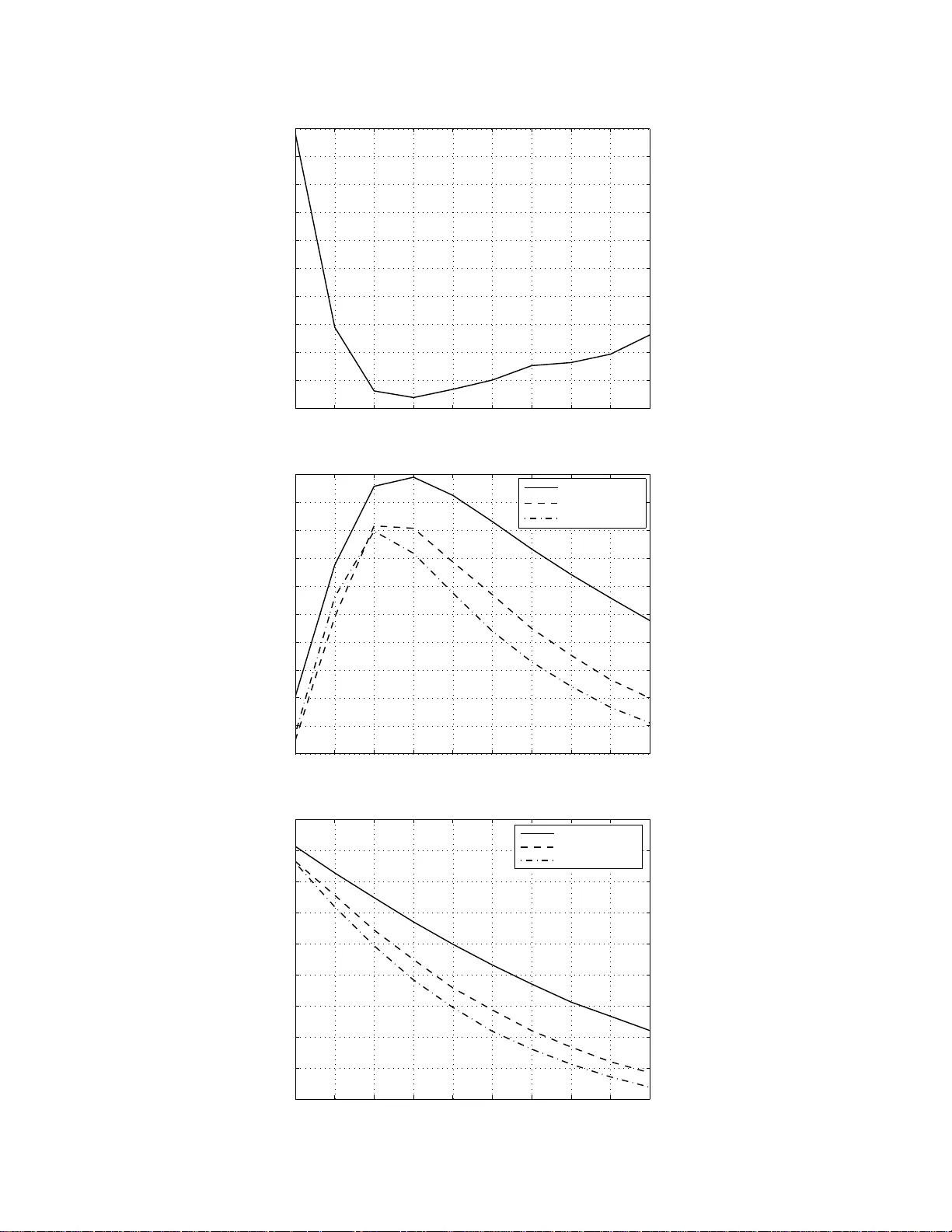
Asymptoticall y Indep enden t Mark o v Sampling: a new M CMC sc heme for Ba y esian I nference James L. Bec k and Konstantin M. Zuev 1 Computing and Mathematical Sciences, Division of Engineering a nd Applied Science, California Institute o f T echnology , USA Abstract In Ba yesia n statistics, man y pr oblems can b e expressed as the ev aluation of the exp ectation of a quan tity of in terest with r esp ect to the p osterior distribution. Stan- dard Mon te C arlo metho d is often not applicable b ecause the encounte r ed p osterior distributions cannot b e sampled d irectly . In this case, the m ost p opular strategies are the imp ortance sampling metho d, Mark o v c hain Mon te Carlo, and ann ealing. In this pap er, w e in tro d uce a new sc heme for Ba y esian infer en ce, called Asymptotically Indep enden t Marko v Sampling (AIMS), whic h is based on th e ab o v e metho ds. W e deriv e imp ortan t ergodic prop erties of AIMS. In particular, it is sho wn that, under certain conditions, the AIMS algorithm pro duces a uniformly ergo dic Mark o v chai n . The c hoice of the free parameters of the algo r ithm is discussed and recommenda- tions are pro vided for this c h oice, b oth theoretically and heuristically based. The eﬃciency of AIMS is demonstrated with three numerical examples, whic h in clude b oth m ulti-mo dal and higher-dimensional target p osterior distribu tions. KEY WORDS: Mark ov c hain Mon te Carlo, Imp ort a nce Sampling, Sim ulated Anneal- ing, Bay esian Inference. 1 Three corn erstones of computational Ba y esian inference In Ba y esian statistics, man y problems can b e expresse d as the ev aluat io n of the ex p ecta- tion of a quan tity of in terest with respect to the p osterior distribution. Standard Mon te Carlo sim ulat io n [MU49], where exp ectations are estimated b y sample a v erages ba sed on samples drawn indep enden tly from the p osterior, is often not applicable b ecause the en- coun tered p osterior distributions are m ulti-dimensional non-G aussian distributions that cannot be explicitly normalized. In this case, the most p opular strategies are imp orta nce sampling and Mark ov c hain Monte Carlo methods. W e brieﬂy review these tw o metho ds ﬁrst b ecause they pla y an imp ortant role in the new MCMC metho d in tro duced in this pap er. Imp ortanc e s ampling : This is nearly as old as the Monte Carlo metho d (see, for instance, [KM53]), and w orks as follo ws. Supp ose w e w an t to ev aluate E π [ h ] that is an exp ectatio n of a function of in terest h : Θ → R under distribution 2 π ( · ) deﬁned o n a parameter space Θ ⊆ R d , E π [ h ] = Z Θ h ( θ ) π ( θ ) dθ . (1) Supp ose also that w e are not able to sample directly fr om π ( · ), although we can compute π ( θ ) for an y θ ∈ Θ to within a prop ort io nalit y constan t. Instead, we sample from some 1 Both authors contributed equally to this w o rk. Cor r esp onding author’s email: zuev@caltech.edu. 2 Unless otherwise stated, all probability distr ibutions are a ssumed to ha ve densities with resp ect to Leb esgue measure, π ( dθ ) = π ( θ ) dθ . F or simplicity , the same symbol will b e used to de no te b oth the distribution and its density , and w e write θ ∼ π ( · ) to deno te that θ is distributed accor ding to π ( · ). 1 other distribution q ( · ) on Θ whic h is readily computable for an y θ ∈ Θ. Let θ (1) , . . . , θ ( N ) b e N i.i.d. samples from q ( · ), and w ( i ) = π ( θ ( i ) ) /q ( θ ( i ) ) denote the im p ortanc e we ight of the i th sample, then we can estimate E π [ h ] b y ˆ h N = P N i =1 w ( i ) h ( θ ( i ) ) P N i =1 w ( i ) . (2) The estimator ˆ h N con v erges almost surely as N → ∞ to E π [ h ] b y the Strong La w of Large Num b ers for any c hoice of distribution q ( · ), provided supp( π ) ⊆ supp( q ). Note that the la tter condition automatically holds in Ba y esian up dating using data D where q ( θ ) = π 0 ( θ ) is the prio r densit y and π ( θ ) ∝ π 0 ( θ ) L ( θ ) is the p osterior p ( θ |D ), where L stands for the lik eliho o d function p ( D | θ ). The estimator ˆ h N in (2) generally has a smaller mean square error than a more straight- forw ard un biased imp o rtance sampling estimator: ˆ h ′ N = 1 N N X i =1 w ( i ) h ( x ( i ) ) . (3) This is esp ecially clear when h is nearly a constant: if h ≈ c , then ˆ h N ≈ c , while ˆ h ′ N has a larger v ariation. Although ˆ h N is biased for a n y ﬁnite N , the bia s can be made small b y taking suﬃcien tly large N , and the improv ement in v ariance makes it a preferred alternativ e to ˆ h ′ N [Li01, RC04]. Another ma jor a dv antage of using ˆ h N instead of ˆ h ′ N , whic h is esp ecially imp orta n t for Ba yes ian applications, is that in using the former we need to kno w π ( θ ) only up to a multiplicativ e normalizing constant; whereas in the latt er, this constan t m ust b e kno wn exactly . The accuracy of ˆ h N dep ends critically on the c hoice of the imp ortanc e sampling d i s - tribution (ISD) q ( · ), whic h is also called the instrumental or trial distribution. If q ( · ) is c hosen carelessly such that the the imp ortance we ig hts w ( i ) ha v e a large v aria tion, then ˆ h N is essen tia lly based only on the few samples θ ( i ) with the largest w eigh ts, yielding generally a v ery p o or estimate. Hence, for importa nce sampling to w or k eﬃcien tly , q ( · ) m ust b e a go o d appro ximation of π ( · ) — “the imp o rtance sampling densit y should mimic the p osterior densit y” [Ge89] — so that the v ariance v ar q [ w ] is not large. Since usually the prior and p osterior a re quite diﬀeren t, it is, therefore, highly ineﬃcien t to use the prior as the imp ortance sampling distribution. When Θ is hig h- dimensional, and π ( · ) is complex, ﬁnding a g o o d imp ort ance sampling distribution can b e v ery challenging, limiting the applicabilit y of the metho d [AB03 ]. F or the estimator ˆ h ′ N in (3), it is not diﬃcult to show that the optimal impo rtance sampling dens ity , i.e., q ∗ ( · ) that minimizes the v ariance of ˆ h ′ N , is q ∗ ( θ ) ∝ | h ( θ ) | π ( θ ). This result is sometime s at t r ibuted to Rubinstein [Ru81], alt ho ugh it w as pro ve d earlier b y Kahn and Marshall [KM53 ]. It is not true, ho w eve r, that q ∗ ( · ) is optimal for the estimator ˆ h N . Note also that this optimalit y resu lt is not useful in practice, since when h ( θ ) ≥ 0, the required normalizing constan t of q ∗ ( · ) is R Θ h ( θ ) π ( θ ) dθ , the in tegral of inte rest. MCMC Sampl i n g : Instead of generating indep enden t samples from an ISD , w e could generate dep enden t samples by sim ulating a Mark o v chain whose state distribution con- v erges to the p osterior distribution π ( · ) as its stationary distribution. Markov chain Monte Ca rl o sampling (MCMC) originated in statistical ph ysics, and no w is widely used in solving statistical problems [Ne93, GRS96, Li01, R C04]. 2 The Metrop olis-Hastings algorithm [MR 2 T 2 53, Ha70], the most p o pula r MCM C tec h- nique, w orks a s follows . Let q ( · | θ ) b e a distribution on Θ, which ma y or ma y not dep end on θ ∈ Θ. Assume that q ( ·| θ ) is easy to sample from and it is either com- putable (up t o a m ultiplicative constan t) or symme tric, i.e. q ( ξ | θ ) = q ( θ | ξ ). T he sam- pling distribution q ( ·| θ ) is called the pr op osal distribution . Starting from essen tially an y θ (1) ∈ supp( π ), the Metrop olis-Hastings algorithm pro ceeds b y iterating the following t w o steps. First, generate a c andidate state ξ from the pro p osal densit y q ( ·| θ ( n ) ). Sec - ond, either accept ξ as the nex t state of the Mark ov c hain, θ ( n +1) = ξ , with probabilit y α ( ξ | θ ( n ) ) = min n 1 , π ( ξ ) q ( θ ( n ) | ξ ) π ( θ ( n ) ) q ( ξ | θ ( n ) ) o ; or reject ξ and set θ ( n +1) = θ ( n ) with the remaining probabilit y 1 − α ( ξ | θ ( n ) ). It can be sho wn (see, for example, [R C04]) , that under fairly w eak conditions, π ( · ) is the stationary distribution of the Mark ov c hain θ (1) , θ (2) , . . . and lim N → ∞ 1 N N X i =1 h ( θ ( i ) ) = Z Θ h ( θ ) π ( θ ) dθ . (4) Since the c hain needs some time (so called “burn- in” p erio d) t o con v erge to stationarity , in practice, an initia l p ortio n of, sa y , N 0 states is usually discarded and ˜ h N = 1 N − N 0 N X i = N 0 +1 h ( θ ( i ) ) (5) is used as a n estimator for E π [ h ]. The tw o main sp ecial cases of the Metrop olis-Hastings alg orithm a re Indep enden t Metrop olis-Hastings (IMH), where the prop osal distribution q ( ξ | θ ) = q g ( ξ ) is indep endent of θ (so q g is a glob al pr op osal ), and Random W alk Metropo lis-Hastings (R WMH), where the prop osal distribution is of t he form q ( ξ | θ ) = q l ( ξ − θ ), i.e. a candidate state is pro p osed as ξ = θ ( n ) + ǫ n , where ǫ n ∼ q l ( · ) is a random p erturbation (so q l is a lo c al pr op osal ). In b oth cas es, the c hoice of the prop osal distribution strong ly aﬀec ts the eﬃciency of the algorithms. F or IMH to w ork w ell, as with impo rtance sampling, the prop osal distribution m ust b e a go o d approx imatio n of the tar get distribution π ( · ), otherwise a large fraction of the candidate samples will be rejected and the Mark o v chain will b e to o slow in co vering the imp ortant regions for π ( · ) . When, ho wev er, it is p ossible to ﬁnd a prop osal q g ( · ), suc h that q g ( · ) ≈ π ( · ), IMH should alw ays be preferred to R WMH b ecause of better eﬃciency , i.e. b etter approxim a t ions of E π [ h ] for a giv en n um b er of samples N . Unfortunately , suc h a prop osal is diﬃcult to construct in the con text of Ba ye sian inference where the p osterior π ( · ) is often complex and high-dimensional. This limits the applicabilit y of IMH. Since the random walk propo sal q l ( · ) is lo cal, it is les s sensitiv e to the target distri- bution. That is wh y , in pr a ctice, R WMH is more robust and used more f r equen t ly than IMH. Nonetheless, there are settings where R WMH also do es not w ork w ell b ecause o f the complexity of the p o sterior distribution. Although (4) is true in theory , a p oten tial problem with R WMH (and, in fact, with any MCMC algorit hm) is that the generated samples θ (1) , . . . , θ ( N ) often consist of highly cor r elat ed samples. T herefore, the estima- tor ˜ h N in (5) obtained from these samples tends to hav e a large v ariance for a mo dest amoun t of sample s. This is esp ecially true when the po sterior distribution contains sev- eral widely-separated mo des: a c hain will mov e b etw een mo des only ra r ely and it will tak e a long time b efore it reac hes stationarit y . If this is the case, an estimate pro duced 3 b y ˜ h N will b e v ery inaccurate. A t ﬁrst g la nce, it seems natural to generate sev eral in- dep enden t Mark ov c hains, starting from diﬀeren t r a ndom seeds, and hop e that diﬀeren t c hains will g et trapp ed b y diﬀerent mo des. How ev er, m ultiple runs will not in general generate a sample in whic h eac h mo de is corr ectly represen ted, since the probabilit y o f a c hain reac hing a mo de dep ends more on the mode’s “basin of attraction” than on the probabilit y concen trated in the mo de [Ne96 ]. A nne aling: The concept o f anne a ling (or temp ering ), whic h inv olv es mo ving from an easy-to-sample distribution to the target distribution via a seq uence o f in termediate distributions, is one of the most eﬀectiv e metho ds of handling m ultiple isolated mo des. T ogether with imp ortance sampling a nd MCMC, annealing constitutes the third corner- stone of computational Bay esian inference. The idea of using the R WMH algorithm in conjunction with annealing w as introduced indep enden tly in [KGV83] and [ ˇ Ce85] for solving diﬃcult optimization problems. The resulting algor ithm, called Simulate d Anne aling , works as fo llo ws. Supp ose we w an t to ﬁnd the glo ba l minimum o f a function of in terest h : Θ → R . This is equiv alent to ﬁnding the global maxim um of f T ( θ ) = exp( − h ( θ ) /T ) for any given T > 0. By analogy with the Gibbs distribution in statistical mec hanics, T is called the tem p er atur e p ar ameter . L et T 0 > T 1 > . . . b e a sequence of monotonically decreasing temp eratures, in which T 0 is large enough so tha t the probabilit y distribution π 0 ( θ ) ∝ f T 0 ( θ ) is close to uniform, and lim j →∞ T j = 0 . A t eac h temp erature T j , the Simulated Annealing metho d generates a Mark o v c hain with π j ( θ ) ∝ exp( − h ( θ ) / T j ) a s its stationary distribution. The ﬁnal state of the Mark ov c hain at sim ula tion lev el j is used as the initial state for the c hain at lev el j + 1. The k ey observ a t io n is that for an y function h suc h that R Θ exp( − h ( θ ) /T ) dθ < ∞ for all T > 0, distribution π j ( · ), as j increases, puts more and more of its pro ba bility mass (con v erging to 1) in to a neigh b orho o d of the global minim um of h . Therefore, a sample dra wn f rom π j ( · ) w ould almost surely b e in a vicinit y of the global minim um of h when T j is close to zero. The success of Simulated Annealing in ﬁnding t he global minimum crucially dep ends on the sc hedule of temp eratures use d in t he sim ulation. It w as pro v ed in [G G84] tha t if a loga rithmic sc hedule T j = T 0 / log( j + 1) is used, then, under certain conditions, there exists a v alue fo r T 0 suc h that use of this sc hedule guarantee s that the global minimum of h will be reac hed almost surely . In practice, ho w ev er, suc h a slo w annealing sc hedule is not computationally eﬃcie nt. It is more common to use either a g eometric sche dule, T j +1 = γ T j with 0 < γ < 1, or some adaptiv e sc hedule, whic h deﬁnes the temperature for the nex t annealing lev el based on c haracteristics of the samples observ ed at earlier lev els. F or examples of adaptiv e a nnealing sc hedules, see, for instance, [Ne93 ]. In Ba y esian inference problems, the idea of annealing is typic ally emplo y ed in the follo wing w ay . First, w e construct (in adv ance or adaptiv ely) a sequence o f distributions π 0 ( · ) , . . . , π m ( · ) interpolating betw een the prior distribution π 0 ( · ) and the p osterior distri- bution π ( · ) ≡ π m ( · ). Next, we generate i.i.d. samples θ (1) 0 , . . . , θ ( N ) 0 from the prio r , whic h is assumed to b e readily sampled. Then, at eac h annealing lev el j , using some MCMC algorithm and samples θ (1) j − 1 , . . . , θ ( N ) j − 1 from the previous lev el j − 1 , w e g enerate samples θ (1) j , . . . , θ ( N ) j whic h are appro ximately distributed according to π j ( · ). W e pro ceed sequen- tially in this w ay , un til the p osterior distribution has b een sampled. The rationale b ehind this strategy is that sampling from the multi-modal a nd, p erhaps, high-dimensional p os- terior in suc h a w ay is lik ely to be more eﬃcien t than a straigh tfo rw ard MCMC sampling 4 of the p osterior. The problem of sampling a complex distribution is encoun tered in statistical mec han- ics, computational Bay esian inf erence, scien tiﬁc computing, mac hine learning, a nd other ﬁelds. As a result, man y diﬀerent eﬃcien t a lgorithms ha ve b een recen tly dev elop ed, e.g. the metho d of Simu la t ed T emp ering [MP92 , GT95], t he T emp ered T r ansition metho d [Ne96], Annealed Imp ort a nce Sampling [Ne01], t he Adaptiv e Metrop olis-Hastings a lg o- rithm [BA02], T ransitional Marko v Chain Mon te Carlo metho d [CC07], to name a few. In this pap er w e in tro duce a new MCMC sc heme for Ba ye sian inference, called Asymp- totic al ly I n dep en d ent Markov Sampling (AIMS), whic h com bines the three approac hes described ab ov e — imp ortance sampling, MCMC , and annealing — in the following w ay . Imp ortance sampling with π j − 1 ( · ) as the ISD is used for a construction of an a pproxima- tion ˆ π N j ( · ) of π j ( · ), whic h is based on samples θ (1) j − 1 , . . . , θ ( N ) j − 1 ∼ π j − 1 ( · ). This approximation is then employ ed a s the indep enden t (global) prop osal distribution for sampling from π j ( · ) b y the IMH algor it hm. In termediate distributions π 0 ( · ) , . . . , π m ( · ) in terp olating b et w een prior and p osterior are constructed adaptiv ely , using the essen tial sample size (ESS) to measure how m uc h π j − 1 ( · ) diﬀers from π j ( · ). When the n umber of samples N → ∞ , the appro ximation ˆ π N j ( · ) conv erges to π j ( · ), pro viding the optimal prop o sal distribution. In other words, when N → ∞ , the corresp onding MCMC sampler pro duces indep enden t samples, hence the name of the algorithm. R emark 1 . The term “Marko v sampling” has sev eral diﬀerent meanings. In this pap er it is used as synony mous to “MCMC sampling”. In this in tro ductory section, w e hav e described all the main ingredien ts that w e will need in the subseq uent sections. The rest of the pap er is organized as follows. In Section 2, the AIMS algorithm is describ ed. The ergo dic prop erties of AIMS a re deriv ed in Section 3. The eﬃciency of AIMS is illustrated in Section 4 with three n umerical examples that include b oth multi-modal and hig h-dimensional p o sterior distributions. Concluding remarks are made in Section 5. 2 Asymptotically Indep enden t Mark o v Sampling Let π 0 ( · ) and π ( · ) b e the prior and the p osterior distributions deﬁned on a parameter space Θ, resp ectiv ely , so that, according to Bay es’ Theorem, π ( θ ) ∝ π 0 ( θ ) L ( θ ), where L denotes the likelihoo d function for data D . Our ultimate go a l is to draw samples that are distributed according t o π ( · ). In Asymptotically Indep enden t Mar ko v Sampling (AIMS), we sequen tially generate samples from in termediate distributions π 0 ( · ) , . . . , π m ( · ) in terp ola ting b et w een the prior π 0 ( · ) and the p osterior π ( · ) ≡ π m ( · ). The sequence of distributions could b e sp ecially constructed for a giv en problem but t he fo llowing sc heme [Ne01, CC07] generally yields go o d eﬃciency: π j ( θ ) ∝ π 0 ( θ ) L ( θ ) β j , (6) where 0 = β 0 < β 1 < . . . < β m = 1. W e will refer to j and β j as the ann e aling level a nd the anne a ling p ar ameter at lev el j , respectiv ely . In the next subsec tio n, w e a ssume that β j is giv en and therefore the intermed ia t e distribution π j ( · ) is also kno wn. In Subsection 2.2, w e describe ho w t o c ho o se the annealing para meters adaptiv ely . 5 2.1 AIMS at annealing lev el j Our ﬁrst goal is to describ e ho w AIMS generates sample θ (1) j , . . . , θ ( N j ) j from π j ( · ) based on the sample θ (1) j − 1 , . . . , θ ( N j − 1 ) j − 1 ∼ π j − 1 ( · ) obtained at the previous annealing lev el. W e start with an informal motiv ating discussion that leads to the sim ula tion algorithm. In Section 3, w e rig o rously prov e tha t t he corres p onding algorithm indeed generates samples whic h are asymptotically distributed according to π j ( · ), as the sample size N j → ∞ . Moreo v er, the larger N j − 1 , the less correlated generated samples θ (1) j , . . . , θ ( N j ) j are — a v ery desirable, y et rarely aﬀordable, prop erty for an y MCMC algorithm. Let K j ( ·|· ) b e any t r a nsition k ernel such that π j ( · ) is a stationary distribution with resp ect to K j ( ·|· ). By deﬁnition, this means that π j ( θ ) dθ = Z Θ K j ( dθ | ξ ) π j ( ξ ) dξ (7) Applying imp orta nce sampling with the sampling densit y π j − 1 ( · ) to in tegral (7), we hav e: π j ( θ ) dθ = Z Θ K j ( dθ | ξ ) π j ( ξ ) π j − 1 ( ξ ) π j − 1 ( ξ ) dξ ≈ N j − 1 X i =1 K j ( dθ | θ ( i ) j − 1 ) ¯ w ( i ) j − 1 def = ˆ π N j − 1 j ( dθ ) , (8) where ˆ π N j − 1 j ( · ) will b e used as the glob al pr op osal distribution in the Indep enden t Metrop olis- Hastings algorithm, a nd w ( i ) j − 1 = π j ( θ ( i ) j − 1 ) π j − 1 ( θ ( i ) j − 1 ) ∝ L ( θ ( i ) j − 1 ) β j − β j − 1 and ¯ w ( i ) j − 1 = w ( i ) j − 1 P N j − 1 k =1 w ( k ) j − 1 (9) are the importa nce w eigh ts and normalized imp ortance w eights, resp ectiv ely . Note that to calculate ¯ w ( i ) j − 1 , w e do not nee d to kno w the no r ma lizing constan ts of π j − 1 ( · ) and π j ( · ). If a dj a cen t in termediate distributions π j − 1 ( · ) and π j ( · ) are suﬃcien tly close (in other w ords, if ∆ β j = β j − β j − 1 is small enough), then the import a nce w eights (9) will not v a r y wildly , and, therefore, we can expect that, for reasonably la rge N j − 1 , approximation (8) is accurate. R emark 2 . In [CB10], the stationary condition (7) w as used for an analytical approxima- tion of the t a rget PDF to ev aluate the evidence (marginal lik eliho o d) for a mo del. R emark 3 . Note that for an y ﬁnite N j − 1 , distribution ˆ π N j − 1 j ( · ) will usually ha v e b oth con tin uous a nd discrete parts. This follows fr om the fact that the tra nsition k ernel in Mark o v chain sim ulation us ually has the f ollo wing form: K ( dθ | ξ ) = k ( θ | ξ ) dθ + r ( ξ ) δ ξ ( dθ ), where k ( ·|· ) describ es the con tinuous part of the transition kerne l, δ ξ ( · ) denotes the Dirac mass at ξ , and r ( ξ ) = 1 − R Θ k ( θ | ξ ) d θ . This is the form, for example, for the Metrop olis- Hastings algorithm. Therefore, (8) m ust b e understoo d as t he appro ximate equalit y of distributions, not densities. In o ther w o r ds, (8) means that E ˆ π N j − 1 j [ h ] ≈ E π j [ h ] and E ˆ π N j − 1 j [ h ] → E π j [ h ], when N j − 1 → ∞ , for all integrable functions h . See also Example 2.1 b elo w. 6 F rom now on, w e consider a sp ecial case where K j ( ·|· ) is the random w alk Metropo lis- Hastings (R WMH) transition k ernel. In this case, it can b e written a s follo ws: K j ( dθ | ξ ) = q j ( θ | ξ ) min  1 , π j ( θ ) π j ( ξ )  dθ + (1 − a j ( ξ )) δ ξ ( dθ ) , (10) where q j ( ·| ξ ) is a symmetric lo c al prop osal densit y , and a j ( ξ ) is the pro ba bilit y of ha ving a prop er tra nsition ξ to Θ \ { ξ } : a j ( ξ ) = Z Θ q j ( θ | ξ ) min  1 , π j ( θ ) π j ( ξ )  dθ (11) Example 2. 1 . As a simple illustration of (8), consider the case wh en π j ( · ) = N ( ·| 0 , 1), π j − 1 ( · ) = N ( ·| 0 , 2), and q j ( ·| ξ ) = N ( ·| ξ , 1 / 2), where N ( ·| µ , σ 2 ) denotes the Gaussian densit y with mean µ a nd v aria nce σ 2 . The approx imatio n ˆ π N j − 1 j ( · ) based on the samples θ (1) j − 1 , . . . , θ ( N j − 1 ) j − 1 ∼ N ( · | 0 , 2) is sho wn in the top panels of Figure 1, fo r N j − 1 = 5 and N j − 1 = 50. Suppo se that h 1 ( θ ) = θ and h 2 ( θ ) = θ 2 are the functions of in terest. Th en E π j [ h 1 ] = 0 and E π j [ h 2 ] = 1. The con v ergence of h ∗ 1 ( N j − 1 ) = E ˆ π N j − 1 j [ h 1 ] and h ∗ 2 ( N j − 1 ) = E ˆ π N j − 1 j [ h 2 ] is sho wn in the b ottom panel of Figure 1 . F or sampling from π j ( · ), w e will use the Inde p enden t Metrop olis-Hastings algorithm (IMH) with the glob al prop osal distribution ˆ π N j − 1 j ( · ). T o a ccomplish this, w e hav e t o b e able to calculate the ratio ˆ π N j − 1 j ( θ ) / ˆ π N j − 1 j ( ξ ) for any θ , ξ ∈ Θ as a part of the expression for the acceptance probabilit y α j ( ξ | θ ) = min  1 , π j ( ξ ) ˆ π N j − 1 j ( θ ) π j ( θ ) ˆ π N j − 1 j ( ξ )  . How ev er, as it has b een already men tio ned, the distribution ˆ π N j − 1 j ( · ) do es not ha ve a densit y since it has b oth con tin uous and discrete comp onen ts, a nd, therefore, the ratio ˆ π N j − 1 j ( θ ) / ˆ π N j − 1 j ( ξ ) ma kes no sense. T o o verc ome this “lac k-o f-con tinuit y problem”, taking in to accoun t (8 ) and (10), let us form a l ly deﬁne the global prop osal distribution ov er Θ as: ˆ π N j − 1 j ( θ ) def = N j − 1 X i =1 ¯ w ( i ) j − 1 q j ( θ | θ ( i ) j − 1 ) min ( 1 , π j ( θ ) π j ( θ ( i ) j − 1 ) ) , (12) if θ / ∈ n θ (1) j − 1 , . . . , θ ( N j − 1 ) j − 1 o , and ˆ π N j − 1 j ( θ ( k ) j − 1 ) def = ∞ (13) Note tha t ˆ π N j − 1 j ( · ) is a distribution on Θ , but it do es not hav e a densit y . How ev er, ˆ π N j − 1 j ( · ) induces another distribution on Θ \ n θ (1) j − 1 , . . . , θ ( N j − 1 ) j − 1 o whic h do es hav e a densit y , giv en b y the r.h.s. of (12). This motiv ates (12). No w, using (12) and (13), we can calculate the ratio ˆ π N j − 1 j ( θ ) / ˆ π N j − 1 j ( ξ ) as follows : I. If θ , ξ / ∈ n θ (1) j − 1 , . . . , θ ( N j − 1 ) j − 1 o , then ˆ π N j − 1 j ( θ ) ˆ π N j − 1 j ( ξ ) = P N j − 1 i =1 ¯ w ( i ) j − 1 q j ( θ | θ ( i ) j − 1 ) min  1 , π j ( θ ) π j ( θ ( i ) j − 1 )  P N j − 1 i =1 ¯ w ( i ) j − 1 q j ( ξ | θ ( i ) j − 1 ) min  1 , π j ( ξ ) π j ( θ ( i ) j − 1 )  (14) 7 I I. If θ / ∈ n θ (1) j − 1 , . . . , θ ( N j − 1 ) j − 1 o and ξ = θ ( k ) j − 1 , then ˆ π N j − 1 j ( θ ) ˆ π N j − 1 j ( ξ ) = 0 and α j ( ξ | θ ) = 0 (15) I I I. If θ = θ ( k ) j − 1 and ξ / ∈ n θ (1) j − 1 , . . . , θ ( N j − 1 ) j − 1 o , then ˆ π N j − 1 j ( θ ) ˆ π N j − 1 j ( ξ ) = ∞ and α j ( ξ | θ ) = 1 (16) IV. If θ = θ ( k ) j − 1 and ξ = θ ( l ) j − 1 , then ˆ π N j − 1 j ( θ ) ˆ π N j − 1 j ( ξ ) is not deﬁned. Notice that in the ﬁrst three cases the r atio ˆ π N j − 1 j ( θ ) / ˆ π N j − 1 j ( ξ ) is readily computable, while in Case IV, it is not ev en deﬁned. Therefore, it is ve ry desirable to av oid Case IV. The ke y observ a tion that allo ws us to do this is t he follo wing: supp ose that the initial state θ (1) j of the Marko v c hain that is generated is suc h that θ (1) j ∈ Θ ∗ j def = Θ \ n θ (1) j − 1 , . . . , θ ( N j − 1 ) j − 1 o , then θ ( i ) j ∈ Θ ∗ j for all i ≥ 1. Indeed, the o nly w ay for the chain to en ter the set n θ (1) j − 1 , . . . , θ ( N j − 1 ) j − 1 o is to generate a candidat e state ξ ∈ n θ (1) j − 1 , . . . , θ ( N j − 1 ) j − 1 o ; ho w eve r, according to Case I I, suc h a candidate will alw ay s b e rejected. Thus , by replacing the state space Θ by Θ ∗ j and using (1 4) and (15) fo r ev aluation of ˆ π N j − 1 j ( θ ) / ˆ π N j − 1 j ( ξ ), w e are a ble to calculate the acceptance probabilit y α j ( ξ | θ ) = min  1 , π j ( ξ ) ˆ π N j − 1 j ( θ ) π j ( θ ) ˆ π N j − 1 j ( ξ )  in v olved in the IMH algorithm. It is clear that the replacemen t of Θ b y Θ ∗ j is harmless fo r the ergo dic prop erties of the Mark ov c hain when Θ ⊆ R d . R emark 4 . One ma y w onder wh y not j ust use the contin uous part of ˆ π N j − 1 j ( · ) as the global prop osal densit y within the IMH algorithm. In other w ords, why not use the densit y ˆ π N j − 1 j, cont ( · ), whic h is pr o p ortional to the function deﬁned b y (1 2), a s the prop osal densit y . Indeed, in this case w e would not ha v e an y diﬃculties with calculating the ratio ˆ π N j − 1 j ( θ ) / ˆ π N j − 1 j ( ξ ). The problem is that it is not cle ar ho w to sample from ˆ π N j − 1 j, cont ( · ), while sampling from ˆ π N j − 1 j ( dθ ) = P N j − 1 i =1 ¯ w ( i ) j − 1 K j ( dθ | θ ( i ) j − 1 ) is straightforw ard. The ab ov e discussion leads to the follo wing algorithm for sampling from the distribu- tion π j ( · ): AIMS at an nealing level j Input: ⊲ θ (1) j − 1 , . . . , θ ( N j − 1 ) j − 1 ∼ π j − 1 ( · ), samples generated at annealing lev el j − 1; ⊲ θ (1) j ∈ Θ ∗ j = Θ \ n θ (1) j − 1 , . . . , θ ( N j − 1 ) j − 1 o , initial state of a Mark ov c hain; ⊲ q j ( ·| ξ ), symmetric prop o sal densit y asso ciated with the R WMH k ernel; ⊲ N j , total num b er of Marko v c hain stat es to b e generated. Algorithm: for i = 1 , . . . , N j − 1 do 1) Generate a global candidate state ξ g ∼ ˆ π N j − 1 j ( · ) as follows: 8 a. Select k from { 1 , . . . , N j − 1 } with probabilities ¯ w ( i ) j − 1 giv en b y (9). b. Generate a lo cal candidate ξ l ∼ q j ( ·| θ ( k ) j − 1 ). c. Accept o r r eject ξ l b y setting ξ g =    ξ l , with probability min  1 , π j ( ξ l ) π j ( θ ( k ) j − 1 )  ; θ ( k ) j − 1 , with the remaining probabilit y . (17) 2) Up date θ ( i ) j → θ ( i +1) j b y accepting or rejecting ξ g as follows : if ξ g = θ ( k ) j − 1 Set θ ( i +1) j = θ ( i ) j else Set θ ( i +1) j =    ξ g , with probability min  1 , π j ( ξ g ) ˆ π N j − 1 j ( θ ( i ) j ) π j ( θ ( i ) j ) ˆ π N j − 1 j ( ξ g )  ; θ ( i ) j , with the remaining probabilit y . (18) end if end for Output: ◮ θ (1) j , . . . , θ ( N j ) j , N j states of a Marko v c hain with a stationary distribution π j ( · ) Sc hematically , the AIMS algorithm at annealing lev el j is sho wn in Figure 2. The pro of t ha t π j ( · ) is indeed a stationar y distribution for the Mark ov chain generated by AIMS is given in Section 3. R emark 5 . As usually for MCMC algorithms, the fact of conv ergence of a Marko v c hain to its stationary distribution do es not dep end on the initial state; ho w ev er, the sp eed of con v ergence do es. One reasonable wa y to c hose the initial state θ (1) j ∈ Θ ∗ j in practical applications is the fo llo wing: generate θ (1) j ∼ q j ( ·| θ ( k ∗ ) j − 1 ), where k ∗ = a r g max k ¯ w ( k ) j − 1 , i.e. θ ( k ∗ ) j − 1 has the largest no r ma lized imp ortance weigh t. 2.2 The full A IMS pro cedure A t the zero th annealing lev el, j = 0, we generate prior samples θ (1) 0 , . . . , θ ( N 0 ) 0 , which usu- ally can b e readily dra wn directly b y a suitable choice of the prio r distribution π 0 ( · ). Then, using t he algorithm describ ed in the previous subsection, we generate samples θ (1) 1 , . . . , θ ( N 1 ) 1 , whic h are appro ximately distributed according to interm ediate distribu- tion π 1 ( θ ) ∝ π 0 ( θ ) L ( θ ) β 1 . W e pro ceed like this un til the p osterior distribution π m ( θ ) ∝ π 0 ( θ ) L ( θ ) β m ( β m = 1) has b een sampled. T o mak e the description of AIMS complete, w e ha v e to explain how to c ho ose the annealing para meters β j , for j = 2 , . . . , m − 1. It is clear tha t the choice of the annealing para meters is ve ry imp orta nt, since, for instance, it a ﬀects the accuracy of the imp ortance sampling a pproximation (8) and, there- fore, the eﬃ ciency of the whole AIMS procedure. At the same time, it is diﬃcult to mak e a rational ch o ice of the β j -v alues in adv ance, since this requires some pr io r knowle dge ab out the p osterior distribution, whic h is often no t a v ailable. F or this reason, w e prop ose an adaptiv e w a y of c ho osing the annealing sc heme. 9 In imp or t a nce sampling, a us eful measure o f degeneracy of the metho d is the eﬀe ctive sample size (ESS) N eﬀ in tro duced in [KL W94 ] a nd [Li96 ]. The ESS measures how similar the imp o rtance sampling distribution π j − 1 ( · ) is to the target distribution π j ( · ). Supp ose N j − 1 indep enden t samples θ (1) j − 1 , . . . , θ ( N j − 1 ) j − 1 are generated f rom π j − 1 ( · ), then the ESS o f these samples is deﬁned as N eﬀ j − 1 = N j − 1 1 + v a r π j − 1 [ w ] = N j − 1 E π j − 1 [ w 2 ] , (19) where w ( θ ) = π j ( θ ) /π j − 1 ( θ ). The ESS can b e interpreted as implying that N j − 1 w eigh ted samples ( θ (1) j − 1 , w (1) j − 1 ) , . . . , ( θ ( N j − 1 ) j − 1 , w ( N j − 1 ) j − 1 ) are w orth N eﬀ j − 1 ( ≤ N j − 1 ) i.i.d. samples drawn from the ta rget distribution π j ( · ). One cannot ev aluate the ESS exactly but a n estimate ˆ N eﬀ j − 1 of N eﬀ j − 1 is giv en b y ˆ N eﬀ j − 1 ( ¯ w j − 1 ) = 1 P N j − 1 i =1 ( ¯ w ( i ) j − 1 ) 2 , (20) where ¯ w j − 1 = ( ¯ w (1) j − 1 , . . . , ¯ w ( N j − 1 ) j − 1 ) and ¯ w ( i ) j − 1 is the normalized imp or t ance w eight of θ ( i ) j − 1 . A t annealing lev el j , when β j − 1 is already kno wn, the problem is to deﬁne β j . Let γ = ˆ N eﬀ j − 1 / N j − 1 ∈ (0 , 1) b e a prescrib ed thresh o ld that c haracterizes the “qualit y” o f the w eigh ted sample (the larger γ is, the “b etter” t he we ig hted sample is). Then w e o btain the follow ing equation: N j − 1 X i =1 ( ¯ w ( i ) j − 1 ) 2 = 1 γ N j − 1 (21) Observ e that this equation can b e express ed as an equation for β j b y using (9): P N j − 1 i =1 L ( θ ( i ) j − 1 ) 2( β j − β j − 1 )  P N j − 1 i =1 L ( θ ( i ) j − 1 ) β j − β j − 1  2 = 1 γ N j − 1 (22) Solving this equation for β j giv es us the v alue of t he annealing parameter at leve l j . R emark 6 . Note that when j ≥ 2, the θ (1) j − 1 , . . . , θ ( N j − 1 ) j − 1 are g enerated b y the Mark ov chain sampler describ ed in the previous subsection and therefore a re not indep enden t. This means that, b ecause of t he auto correlations pro duced b y the Marko v c hain used, the “true” ESS of this sample is, in fa ct, smaller than the one giv en b y (19). This is useful to remem b er when c ho osing γ . Also, this is another r eason to select the prior distribution π 0 ( · ) so that samples can b e generated indep enden tly at the start of eac h AIMS run. Com bining the AIMS alg o rithm a t a giv en annealing lev el with the describ ed adaptive annealing sc heme giv es rise to the followin g pro cedure. The A IMS pro cedure Input: ⊲ γ , threshold for the eﬀectiv e sample size (ESS); ⊲ N 0 , N 1 , . . . , where N j is the total nu mber of Mark ov ch a in states to b e generated at annealing lev el j ; ⊲ q 1 ( ·| ξ ) , q 2 ( ·| ξ ) , . . . , where q j ( ·| ξ ) is the symm etric prop osal densit y asso ciated with the R WMH k ernel at annealing lev el j . 10 Algorithm: Set j = 0, current annealing lev el. Set β 0 = 0, curren t annealing parameter. Sample θ (1) 0 , . . . , θ ( N 0 ) 0 i.i.d ∼ π 0 ( · ). Calculate ¯ W ( i ) 0 = L ( θ ( i ) 0 ) 1 − β 0 P N 0 i =1 L ( θ ( i ) 0 ) 1 − β 0 , i = 1 , . . . , N 0 . Calculate the ESS ˆ N eﬀ 0 = ˆ N eﬀ 0 ( ¯ W 0 ) using (20 ) , which measures how similar the prior distribution π 0 ( · ) is to the tar get p osterior distribution π ( · ). while ˆ N eﬀ j / N j < γ do Find β j +1 from equation (2 2). Calculate normalized imp ortance we ights ¯ w ( i ) j , i = 1 , . . . , N j using (9). Generate a Marko v c hain θ (1) j +1 , . . . , θ ( N j +1 ) j +1 with the stationary distribution π j +1 ( · ) using t he AIMS algorithm at annealing lev el j + 1. Calculate ¯ W ( i ) j +1 = L ( θ ( i ) j +1 ) 1 − β j +1 P N j +1 i =1 L ( θ ( i ) j +1 ) 1 − β j +1 , i = 1 , . . . , N j +1 . Calculate the ESS ˆ N eﬀ j +1 = ˆ N eﬀ j +1 ( ¯ W j +1 ) using (20), which measures ho w similar the in termediate distribution π j +1 ( · ) is to the p osterior π ( · ) . Incremen t j to j + 1. end while Set β j +1 = 1, curren t annealing parameter. Set m = j + 1, the total num b er of distributions in the annealing sc heme. Set ¯ w ( i ) m − 1 = ¯ W ( i ) m − 1 , i = 1 , . . . , N m − 1 . Generate a Marko v c hain θ (1) m , . . . , θ ( N m ) m with the statio nary distribution π m ( · ) = π ( · ) using the AIMS algor ithm at annealing leve l m . Output: ◮ θ (1) m , . . . , θ ( N m ) m ˙ ∼ π ( · ), samples that are a ppro ximately distributed according to the p osterior distribution. 2.3 Implemen tation issues As it follo ws from the description, the AIMS pro cedure has the f ollo wing parameters: γ , the thresh old fo r the eﬀectiv e sample size; N j , the len g t h of a Mark o v c hain generated at annealing lev el j = 1 , . . . , m ; and q j ( ·| ξ ), the symme tr ic prop o sal densit y asso ciated with the R WMH kernel at lev el j = 1 , . . . , m . Here, w e discuss the c hoice of these pa rameters and how this c ho ice aﬀects the eﬃciency o f AIMS. First of all, it is absolutely clear that, as for an y Monte Carlo metho d, the larg er the n um b er of generated samples is, the mo r e accurate the corresp onding estimates of (1) are. Ho w eve r, w e w ould lik e to highligh t the diﬀerence betw een the roles of N j − 1 and N j at annealing lev el j . While N j is directly related to the con v ergence of the c hain θ (1) j , . . . , θ ( N j ) j to its stationary distribution π j ( · ), N j − 1 aﬀects this conv ergence implicitly through the global prop o sal distribution ˆ π N j − 1 j ( · ): the larger N j − 1 , the more accurate approximation (8) is, and, therefore, the less correlated θ (1) j , . . . , θ ( N j ) j are. When N j − 1 → ∞ , samples θ (1) j , . . . , θ ( N j ) j b ecome indep enden t draws from π j ( · ), hence the name of t he a lgorithm. Th us, if w e increase N = N j − 1 = N j , the eﬀect is tw of o ld: ﬁrst, the sample size increases thereb y increasing the eﬀectiv e n um b er of indep enden t samples at the j th lev el (ty pical for 11 an y Monte Carlo metho d); second, the samples b ecome less correlated (a useful feature of AIMS), again increasing the eﬀectiv e num b er of indep enden t samples. As a result of these t w o eﬀects, increasing N has a strong inﬂuence on the eﬀec tive n um b er of independen t p osterior samples and so strongly reduces the v ariance of t he estimator for (1). Supp ose no w that w e are at t he last annealing lev el and generating a Mark ov chain θ (1) m , . . . , θ ( N m ) m with the stationary distribution π m ( · ) = π ( · ). W e will refer to this c hain as the p osterior Marko v c hain. A critical question faced by users of MCM C metho ds is ho w to determine when it is safe t o stop sampling from the p osterior distribution and use samples θ (1) m , . . . , θ ( N m ) m for estimation. In other w or ds, ho w large should N m b e? One p ossible solution of this “ con v ergence assessmen t problem” is to use one of the numer- ous published diagnostic tec hniques; fo r example, see [CC96 ] fo r a compara tiv e r eview of MCMC con v ergence diagnostics. Unfortunately , none of the published diagnostics allo ws one to sa y with certain ty that a ﬁnite sample f r om an MCMC algorithm is represen ta- tiv e o f an underlying stationary distribution. A more empirical approach for assessing con v ergence is to run sev eral p osterior Marko v chains θ (1) k ,m , . . . , θ ( N m ) k ,m , k = 1 , . . . , K , in parallel and monitor the corresponding estimators ˆ h 1 , . . . , ˆ h K of E π [ h ]. A stopping rule for con v ergence is then max 1 ≤ i 0 is a prescrib ed threshold. It is easy to sho w that the ESS-criterion (21) and the COV - criterion (24 ) are mathematically equiv alen t; in f act, ˆ N eﬀ j − 1 = N j − 1 / (1 + δ 2 ). W e prefer to use the former criterio n since γ has a clear meaning: it is the factor b y whic h the (essen tia l) sample size of t he w eigh ted sample is reduced as a p enalt y for sampling from the imp o rtance sampling densit y instead of the target distribution. It has b een found in [CC07] that δ = 1 is usually a reasonable c hoice of the threshold. This corresp onds to γ = 1 / 2. Our sim ulatio n results (see Section 4) a lso sho w that a nnealing sc hemes with γ around 1 / 2 yield g o o d eﬃciency . 12 The choice of the lo cal prop o sal densit y q j ( ·| ξ ) asso ciated with the R WMH kerne l deter- mines the ergo dic prop erties of the Marko v chain generated by AIMS at lev el j ; it also de- termines how eﬃcien tly the ch a in explores lo cal neighborho o ds of samples θ (1) j − 1 , . . . , θ ( N j − 1 ) j − 1 generated at the previous lev el. This mak es the c hoice of q j ( ·| ξ ) v ery imp ortan t. It has been observ ed b y ma ny researc hers that the eﬃciency of Me tr o p olis-Hastings based MCMC metho ds is not sensitiv e to the type of the prop osal densit y; how eve r, it strongly dep ends on its v ariance (e.g. [GRG96, AB01]). F or this reason, w e suggest using a Gaussian densit y as the lo cal prop osal: q j ( θ | ξ ) = N ( θ | ξ , c 2 j I ) , (25) where ξ and c 2 j I are the mean and dia g onal co v ariance matrix, respectiv ely . The scaling parameter c 2 j determines the “spread” of the lo cal prop osal distribution. In Section 3, w e prov e (Theorem 3 ) that , under certain conditions, the acceptance rate ¯ A j (i.e. t he exp ected proba bility of ha ving a pro p er Mark ov transition θ ( i ) j to θ ( i +1) j 6 = θ ( i ) j ) satisﬁes ¯ A j ≥ 1 M , where constan t M dep ends on q j ( ·| ξ ) and, therefore, o n c 2 j . This result can b e p otentially used for ﬁnding an optimal c 2 j that w ould minimize M . Alternativ ely , a more empirical w a y of c ho osing the scaling factor consists of adjusting c 2 j based on the estimated acceptance rate. This works as f o llo ws: ﬁrst, choose an initial v alue for the scaling fa cto r , c 2 j, 0 , and estimate the corresp onding acceptance rate ¯ A j ( c 2 j, 0 ) based on N j generated Mark o v states, then mo dify c 2 j, 0 to obtain an increase in ¯ A j . Whe ther this optimization in c 2 j is useful dep ends on whether the accuracy of the estimator that is ach ieve d comp ensates for the additiona l computational cost. Finally , note that our sim ulation results show (see Section 4) that, as j increases, the corresp onding optimal scaling factor c 2 j decreases slightly . This observ a tion coincides with intuition, since when j increases , the in termediate distributions π j ( · ) b ecome mor e concen trated. In the follo wing section w e establish the ergo dic prop erties of the Mark ov c hains gen- erated b y AIMS. 3 Ergo dic prop erties of AIMS Since the discussion in Subsection 2.1, which motiv at ed AIMS a t annealing lev el j , in- v olv ed delta functions and formal equalities (12) and (13), w e cannot simply rely on the con v ergence o f the IMH alg orithm in v eriﬁcation of AIMS; a rigorous pro of is needed. First w e prov e that the describ ed algorithm indeed generates a Mark ov c hain with a stationary distribution π j ( · ). W e also explain that when the prop osal densit y q j ( ·| ξ ) is reasonably c hosen, π j ( · ) is the unique (and, therefore, limiting) stationary distribution of the corresp onding Marko v c hain. Theorem 1. L et θ (1) j , θ (2) j , . . . b e the Markov chain o n Θ ∗ j = Θ \ n θ (1) j − 1 , . . . , θ ( N j − 1 ) j − 1 o gen- er ate d by the AI MS algorithm at anne aling level j , then π j ( · ) is a stationary distribution of the Markov chain. Pr o of. Let K j ( ·|· ) denote the transition k ernel of the Mark ov chain g enerated b y AIMS at annealing lev el j . F rom the discription of the alg o rithm it fo llo ws that K j ( ·|· ) has the follo wing form: 13 K j ( dξ | θ ) = N j − 1 X i =1 ¯ w ( i ) j − 1 q j ( ξ | θ ( i ) j − 1 ) min ( 1 , π j ( ξ ) π j ( θ ( i ) j − 1 ) ) min ( 1 , π j ( ξ ) ˆ π N j − 1 j ( θ ) π j ( θ ) ˆ π N j − 1 j ( ξ ) ) dξ + (1 − A j ( θ )) δ θ ( dξ ) , (26) where A j ( θ ) is the probabilit y of having a prop er transition θ to Θ ∗ j \ { θ } : A j ( θ ) = Z Θ ∗ j N j − 1 X i =1 ¯ w ( i ) j − 1 q j ( ξ | θ ( i ) j − 1 ) min ( 1 , π j ( ξ ) π j ( θ ( i ) j − 1 ) ) min ( 1 , π j ( ξ ) ˆ π N j − 1 j ( θ ) π j ( θ ) ˆ π N j − 1 j ( ξ ) ) dξ (27) A suﬃcien t condition fo r π j ( · ) to b e a stationary distribution is for K j ( ·|· ) to satisfy the detailed ba la nce condition: π j ( dθ ) K j ( dξ | θ ) = π j ( dξ ) K j ( dθ | ξ ) (28) Without loss o f generalit y , we assume that θ 6 = ξ , since otherwise (28) is t r ivial. In this case K j ( dξ | θ ) is giv en b y the ﬁrst term in (26), since the second term v anishes. Thus , all w e need t o pro v e is that f unction E ( θ , ξ ) def = π j ( θ ) N j − 1 X i =1 ¯ w ( i ) j − 1 q j ( ξ | θ ( i ) j − 1 ) min ( 1 , π j ( ξ ) π j ( θ ( i ) j − 1 ) ) min ( 1 , π j ( ξ ) ˆ π N j − 1 j ( θ ) π j ( θ ) ˆ π N j − 1 j ( ξ ) ) (29) is symmetric with respect to p ermutation θ ↔ ξ , for all θ , ξ ∈ Θ ∗ j . T aking in to accoun t (12) and a simple fact that a min { 1 , b/a } = b min { 1 , a/b } for all a, b > 0, w e ha ve: E ( θ , ξ ) = π j ( θ ) ˆ π N j − 1 j ( ξ ) min ( 1 , π j ( ξ ) ˆ π N j − 1 j ( θ ) π j ( θ ) ˆ π N j − 1 j ( ξ ) ) = π j ( ξ ) ˆ π N j − 1 j ( θ ) min ( 1 , π j ( θ ) ˆ π N j − 1 j ( ξ ) π j ( ξ ) ˆ π N j − 1 j ( θ ) ) = E ( ξ , θ ) (30) This prov es that π j ( · ) is a statio nary distribution of the AIMS Mark ov c hain. A statio na ry distribution is unique and is the limiting distribution for a Mark ov c hain, if the ch a in is ap erio dic and ir r educible (see, f or example, [Ti94]). In the case o f AIMS, ap erio dicity is guaran teed b y the fact that the probabilit y of ha ving a rep eat ed sample θ ( i +1) j = θ ( i ) j is not zero: for example, if the lo cal candidate state ξ l is rejected in step 1c, then w e automatically hav e θ ( i +1) j = θ ( i ) j . A Mark ov c hain with stationary distribution π ( · ) is irreducible if, for any initial state, it has positiv e probabilit y of en tering any set to whic h π ( · ) assigns p ositive probability . It is clear that if the prop osal distribution q j ( ·| ξ ) is “standard” (e.g. Gaussian, uniform, log-normal, etc), then AIMS generates an irreducible Mark o v c hain. In this case, π j ( · ) is therefore the unique stationary distribution of the AIMS Mark ov c hain, a nd for ev ery θ ∈ Θ ∗ j lim n →∞ kK n j ( ·| θ ) − π j ( · ) k TV = 0 , (31) 14 with k · k TV denoting the total v ariation distance. Recall that the total v ariation dis- tance b et w een t wo measures µ 1 ( · ) a nd µ 2 ( · ) on Θ is deﬁned as k µ 1 ( · ) − µ 1 ( · ) k TV = sup A ⊂ Θ | µ 1 ( A ) − µ 2 ( A ) | . In a sim ulat io n setup, the most import a n t consequence o f con- v ergence prop ert y (31) is, of course, that the sample mean conv erges to the exp ectation of a measurable function of in terest almost surely: lim N j →∞ 1 N j N j X i =1 h ( θ ( i ) j ) = Z Θ h ( θ ) π j ( θ ) dθ (32) Con v ergence (31) ensures the prop er b ehav ior o f the AIMS c hain θ (1) j , θ (2) j , . . . regardless of the initial state θ (1) j . A more detailed description o f conv ergence prop erties inv olves the study of the sp eed of con v ergence of K n j ( ·| θ ) to π j ( · ). Ev aluat ion (or estimation) of this speed is v ery imp ortan t for an y MCMC algorithm, since it relates to a stopping rule for this algorithm: the higher the sp eed of conv ergence K n j ( ·| θ ) → π j ( · ), the less samples are need to obtain a n accurate estimate in (32). Recall, following [MT09], that a c hain θ (1) , θ (2) , . . . is called uniformly er go dic if lim n →∞ sup θ ∈ Θ kK n ( ·| θ ) − π ( · ) k TV = 0 (33) The prop ert y of uniform ergo dicity is stronger than (31 ), since it guarantee s that the sp eed of conv ergence is unifo rm ov er the whole space. Moreo v er, a Mark ov c hain is uniformly ergo dic if and only if there exist r > 1 and R < ∞ suc h tha t for all θ ∈ Θ kK n ( ·| θ ) − π ( · ) k TV ≤ R r − n , (34) that is, the con v ergence in (33) takes place at uniform geometric rat e [MT09]. Theorem 2. If ther e exists a c onstant M such that for al l θ ∈ Θ ∗ j π j ( θ ) ≤ M ˆ π N j − 1 j ( θ ) , (35) then the AIMS algorithm at anne aling level j pr o duc es a uniforml y er go dic chain and kK n j ( ·| θ ) − π j ( · ) k TV ≤  1 − 1 M  n (36) Pr o of. T o pro v e the ﬁrst part of the theorem w e will need the notion of a smal l set [MT09]. A set A ⊂ Θ is called a small set if there exists an intege r m > 0 and a non-trivial measure µ m on Θ, suc h that for all θ ∈ A , B ⊂ Θ: K m ( B | θ ) ≥ µ m ( B ) (37) In this case w e sa y that A is µ m -small. It can b e sho wn [MT 09 ] that a Mark ov c hain is uniformly ergo dic if and only if its state space is µ m -small for some m . Thus, to pro v e the theorem, it is enough to sho w that Θ ∗ j is a small set. 15 If (35) is satisﬁed, than the follow ing holds for transition k ernel (26) for θ ∈ Θ ∗ j and B ⊂ Θ ∗ j : K j ( B | θ ) ≥ Z B N j − 1 X i =1 ¯ w ( i ) j − 1 q j ( ξ | θ ( i ) j − 1 ) min ( 1 , π j ( ξ ) π j ( θ ( i ) j − 1 ) ) min ( 1 , π j ( ξ ) ˆ π N j − 1 j ( θ ) π j ( θ ) ˆ π N j − 1 j ( ξ ) ) dξ = Z B ˆ π N j − 1 j ( ξ ) min ( 1 , π j ( ξ ) ˆ π N j − 1 j ( θ ) π j ( θ ) ˆ π N j − 1 j ( ξ ) ) dξ = Z B min ( ˆ π N j − 1 j ( ξ ) , π j ( ξ ) ˆ π N j − 1 j ( θ ) π j ( θ ) ) dξ ≥ Z B min  ˆ π N j − 1 j ( ξ ) , π j ( ξ ) M  dξ = 1 M Z B π j ( ξ ) dξ = 1 M π j ( B ) (38) The sample space Θ ∗ j is therefore π j M -small, and the corresp onding Mark o v chain is uni- formly ergo dic. T o prov e b ound (36), ﬁrst observ e, using (38), that kK j ( ·| θ ) − π j ( · ) k TV = sup A |K j ( A | θ ) − π j ( A ) | ≤ sup A | π j ( A ) − 1 M π j ( A ) | = 1 − 1 M (39) F or n > 1, using the Chapman-K o lmogorov equation K m + n ( A | θ ) = R Θ K m ( A | ξ ) K n ( dξ | θ ) and stationarity of π j ( · ) with resp ect to K j ( ·|· ), w e ha v e: kK n j ( ·| θ ) − π j ( · ) k TV = sup A |K n j ( A | θ ) − π j ( A ) | = sup A      Z Θ ∗ j K j ( A | ξ ) K n − 1 j ( dξ | θ ) − Z Θ ∗ j K j ( A | ξ ) π j ( ξ ) dξ      = sup A      Z Θ ∗ j K j ( A | ξ )  K n − 1 j ( dξ | θ ) − π j ( ξ ) dξ       = sup A      Z Θ ∗ j [ K j ( A | ξ ) − π j ( A )]  K n − 1 j ( dξ | θ ) − π j ( ξ ) dξ       , (40) where the last equality follow s from the fact that R Θ ∗ j K n − 1 j ( dξ | θ ) = R Θ ∗ j π j ( ξ ) dξ = 1. Finally , we obtain: kK n j ( ·| θ ) − π j ( · ) k TV ≤ sup B sup A     Z B [ K j ( A | ξ ) − π j ( A )]  K n − 1 j ( dξ | θ ) − π j ( ξ ) dξ      ≤ sup B     Z B sup A |K j ( A | ξ ) − π j ( A ) |  K n − 1 j ( dξ | θ ) − π j ( ξ ) dξ      = kK j ( ·| θ ) − π j ( · ) k TV · kK n − 1 j ( ·| θ ) − π j ( · ) k TV ≤  1 − 1 M  n (41) R emark 7 . Note tha t if there exists a constant M suc h that (3 5) holds for all θ ∈ Θ ∗ j , then M > 1 a utomatically . 16 Corollary 1. If Θ ⊂ R d is a c omp act set and q j ( ·| ξ ) is a Gaussian distribution c enter e d at ξ , then the AIMS algorithm at anne aling level j pr o duc es a uniformly er go dic chain and (36) holds with M given by M =   N j − 1 X i =1 ¯ w ( i ) j − 1 min θ ∈ Θ q j ( θ | θ ( i ) j − 1 ) max θ ∈ Θ π j ( θ )   − 1 (42) Pr o of. Let us sho w that in this case condition (35) is alw ay s fulﬁlled. F or an y θ ∈ Θ ∗ j w e ha v e: ˆ π N j − 1 j ( θ ) = N j − 1 X i =1 ¯ w ( i ) j − 1 q j ( θ | θ ( i ) j − 1 ) min ( 1 , π j ( θ ) π j ( θ ( i ) j − 1 ) ) = N j − 1 X i =1 ¯ w ( i ) j − 1 q j ( θ | θ ( i ) j − 1 ) π j ( θ ) π j ( θ ( i ) j − 1 ) min ( 1 , π j ( θ ( i ) j − 1 ) π j ( θ ) ) ≥ π j ( θ ) N j − 1 X i =1 ¯ w ( i ) j − 1 min θ ∈ Θ q j ( θ | θ ( i ) j − 1 ) π j ( θ ( i ) j − 1 ) min ( 1 , π j ( θ ( i ) j − 1 ) max θ ∈ Θ π j ( θ ) ) = π j ( θ ) N j − 1 X i =1 ¯ w ( i ) j − 1 min θ ∈ Θ q j ( θ | θ ( i ) j − 1 ) max θ ∈ Θ π j ( θ ) (43) Th us, (3 5 ) holds with M g iv en by (42). R emark 8 . Note than the assumption of compactnes s of the sample space Θ is not v ery restrictiv e and is t ypically satisﬁed in most Ba y esian statistics problems. Indeed, to fulﬁll this condition, it is enough to tak e a prior distribution π 0 ( · ) with compact supp ort. Next, it is clear from the pro of, that the conclusion of Corolla ry 1 holds for diﬀeren t “reasonable” (not only Ga ussian) prop osal distributions q j ( ·| ξ ). Therefore, the AIMS algorithm will pro duce a unifo rmly ergo dic Marko v c hain in man y practical cases. It has b een recognized for a lo ng time that, when using an MCMC algorithm, it is useful to monito r its a cceptance ra te ¯ A , i.e. exp ected probabilit y of having a prop er Mark o v jump θ ( i ) to θ ( i +1) 6 = θ ( i ) . While in the case o f t he R WMH a lgorithm, the ﬁnding of the optimal acceptance rate is a diﬃcult pro blem: neither high no r low ¯ A is go o d [GR G 96]; for IMH the picture is rather simple: the higher ¯ A , the b etter [R C04]. Since AIMS is based on the IMH alg orithm, their prop erties are v ery similar. In particular, one should aim f or the highest p ossible acceptance rate of the global candidate state ξ g when implemen ting AIMS. W e ﬁnish this section with a result that prov ides b o unds for the acceptance rate of the AIMS a lg orithms. These b ounds can b e useful for ﬁnding the optimal implemen tation parameters. Theorem 3. L et ¯ A j b e the exp e cte d pr ob ab ility of having a p r op er Markov tr ansition asso c iate d with the AIMS algorithm at ann e alin g level j . Then ¯ A j ≤ N j − 1 X i =1 ¯ w ( i ) j − 1 a j ( θ ( i ) j − 1 ) , (44) 17 wher e a j ( θ ( i ) j − 1 ) is p r ob ability (11) asso ciate d with havin g a pr op er tr ansition under the R WMH tr ansition kernel (10). If (35) holds, then ¯ A j ≥ 1 M (45) Pr o of. F or ev ery θ ∈ Θ ∗ j , the probability A j ( θ ) of transition θ to Θ ∗ j \ { θ } is giv en by (27). F or its exp ected v alue we ha v e: ¯ A j = Z Θ ∗ j π j ( θ ) A j ( θ ) dθ = Z Θ ∗ j Z Θ ∗ j π j ( θ ) N j − 1 X i =1 ¯ w ( i ) j − 1 q j ( ξ | θ ( i ) j − 1 ) min ( 1 , π j ( ξ ) π j ( θ ( i ) j − 1 ) ) min ( 1 , π j ( ξ ) ˆ π N j − 1 j ( θ ) π j ( θ ) ˆ π N j − 1 j ( ξ ) ) dξ dθ ≤ Z Θ ∗ j Z Θ ∗ j π j ( θ ) N j − 1 X i =1 ¯ w ( i ) j − 1 q j ( ξ | θ ( i ) j − 1 ) min ( 1 , π j ( ξ ) π j ( θ ( i ) j − 1 ) ) dξ dθ = Z Θ ∗ j π j ( θ ) N j − 1 X i =1 ¯ w ( i ) j − 1 a j ( θ ( i ) j − 1 ) dθ = N j − 1 X i =1 ¯ w ( i ) j − 1 a j ( θ ( i ) j − 1 ) (46) T o prov e the lo we r b ound (45), w e use (12) in the equation deﬁning ¯ A j : ¯ A j = Z Θ ∗ j Z Θ ∗ j π j ( θ ) ˆ π N j − 1 j ( ξ ) min ( 1 , π j ( ξ ) ˆ π N j − 1 j ( θ ) π j ( θ ) ˆ π N j − 1 j ( ξ ) ) dξ dθ = Z Θ ∗ j Z Θ ∗ j π j ( θ ) ˆ π N j − 1 j ( ξ ) I π j ( ξ ) ˆ π N j − 1 j ( θ ) π j ( θ ) ˆ π N j − 1 j ( ξ ) ≥ 1 ! dξ dθ + Z Θ ∗ j Z Θ ∗ j π j ( θ ) ˆ π N j − 1 j ( ξ ) I π j ( θ ) ˆ π N j − 1 j ( ξ ) π j ( ξ ) ˆ π N j − 1 j ( θ ) ≥ 1 ! π j ( ξ ) ˆ π N j − 1 j ( θ ) π j ( θ ) ˆ π N j − 1 j ( ξ ) dξ dθ = 2 Z Θ ∗ j Z Θ ∗ j π j ( θ ) ˆ π N j − 1 j ( ξ ) I π j ( ξ ) ˆ π N j − 1 j ( θ ) π j ( θ ) ˆ π N j − 1 j ( ξ ) ≥ 1 ! dξ dθ ≥ 2 Z Θ ∗ j Z Θ ∗ j π j ( θ ) π j ( ξ ) M I π j ( ξ ) ˆ π N j − 1 j ( ξ ) ≥ π j ( θ ) ˆ π N j − 1 j ( θ ) ! dξ dθ = 2 M P π j ( ξ ) ˆ π N j − 1 j ( ξ ) ≥ π j ( θ ) ˆ π N j − 1 j ( θ ) ! = 1 M , (47) where the last probabilit y is equal to 1 / 2, b ecause θ and ξ are i.i.d. according t o π j ( · ), and hence the r esult. R emark 9 . The AIMS algorithm at annealing lev el j has t wo accept/reject steps: one is for the lo cal candidat e ξ l (step 1c) and another is for the global candidate ξ g (step 2 ). The right-hand side of (44) is nothing else but the lo cal acceptance rate, i.e. exp ected probabilit y of generating a prop er lo cal candidate state ξ l / ∈ { θ (1) j − 1 , . . . , θ ( N j − 1 ) j − 1 } . Basically , (44) says that the global acceptance rate ¯ A j can nev er exceed the lo cal acceptance ra te. 18 In fact, it can b e deduced directly from the description of the a lgorithm, since if the lo cal candidate ξ l is rejected, then the global candidate ξ g is automatically rejected and w e ha v e a rep eated sample θ ( i +1) j = θ ( i ) j . 4 Illustrativ e Examples In this section we illustrate the use o f AIMS with three examples: 1) mixture of ten Gaussian distributions in tw o dimensions (a m ulti-mo dal case); 2) sum o f tw o multiv a r ia te Gaussian distributions in higher dimensions; and 3) Ba ye sian up dating of a neural net w ork mo del. 4.1 Multi-mo dal mixture of Gaussians in 2D T o demons tra te the eﬃciency of AIMS for sampling from m ulti-mo dal distributions, con- sider sim ulation from a truncated tw o-dimensional mixture of M Ga ussian densities: π ( θ ) ∝ π 0 ( θ ) · L ( θ ) = U [0 ,a ] × [0 ,a ] ( θ ) · M X i =1 w i N ( θ | µ i , σ 2 I 2 ) , (48) where U [0 ,a ] × [0 ,a ] ( · ) denotes the uniform distribution on the square [0 , a ] × [0 , a ]. In t his example, a = 1 0, M = 10, σ = 0 . 1, w 1 = . . . = w 10 = 0 . 1, and the mean v ectors µ 1 , . . . , µ 10 are dra wn uniformly from t he square [0 , 10] × [0 , 10]. Because of our in terest in Bay esian up dating, w e refer to π ( · ) in (48) as a p osterior distribution. Figure 3(a) display s the scatterplot of 10 3 p osterior samples obtained from AIMS. No- tice there are t w o clusters o f samples t ha t o verlap signiﬁcan tly near θ = (4 , 4) that r eﬂect t w o closely spaced Gaussian densities but the o ther 8 clusters are widely spaced. The parameters of the a lg orithm we re c hosen as follows : sample size N = 10 3 p er annealing lev el; the threshold for the ESS γ = 1 / 2; the lo cal prop osal densit y q j ( ·| ξ ) = N ( · | ξ , c 2 I 2 ), with c = 0 . 2. The tra jectory of the corresp onding p osterior Mark ov c hain, i.e. the chain generated at the last annealing lev el with statio na ry distribution π ( · ), is sho wn in Fig- ure 3(b). Blac k crosses × represen t the mean vec to rs µ 1 , . . . , µ 10 . As exp ected, the c hain do es no t exhibit a lo cal random w alk b ehavior and it mov es freely b et we en w ell-separated mo des of the p osterior distribution. The describ ed implemen tation of AIMS leads to a total n umber of m = 6 in termediate distributions in the annealing sc heme. Figure 4 sho ws how annealing parameter β j c hanges as a function o f j for 50 indep endent runs of t he algorithm. It is found that in all considered examples, β j gro ws exp onentially with j . Let us no w compare the p erfor ma nce of AIMS with the Random W alk Metrop olis- Hastings algor it hm. F or a fa ir comparison, the Metrop olis-Hastings alg orithm w as imple- men ted as f o llo ws. First, a sample of N 0 = 10 3 p oin ts θ (1) 0 , . . . , θ ( N 0 ) 0 w as dra wn from the prior distribution π 0 ( · ) = U [0 ,a ] × [0 ,a ] ( · ) and the corresp onding v alues of the lik eliho o d f unc- tion L ( θ ) = P M i =1 w i N ( θ | µ i , σ 2 I 2 ) w ere calculated, L i = L ( θ ( i ) 0 ). Then, starting fro m the p oin t with the largest lik eliho o d, θ (1) = θ ( k ) 0 , k = arg max L i , a Mark ov c hain θ (1) , . . . , θ ( N ) , with stationary distribution π ( · ) w as generated using the Metropolis-Ha stings algo r it hm. The prop osal distribution used w as q ( ·| ξ ) = N ( ·| ξ , c 2 I 2 ) with c = 0 . 2, and the length of the c hain w as N = 5 · 10 3 . T hus, the total n um b er of samples use d in b oth AIMS and R WMH w a s N t = 6 · 10 3 . The scatterplot of p osterior samples obtained f rom R WMH 19 and the tra jectory of the corresponding Mark o v chain are sho w in F ig ures 3(c) and 3(d), resp ectiv ely . While the AIMS algorithm successfully sample d all 10 mo des with the ap- pro ximately correct prop ortion of total samples, R WHM completely missed 7 mo des. Supp ose that w e are in terested in estimating the p osterior mean v ector, µ π = ( µ π 1 , µ π 2 ), and the comp onen ts ( σ π 1 ) 2 , ( σ π 2 ) 2 , σ π 12 of the p o sterior cov a riance matrix Σ π . Their true v alues are giv en in T able 1 alo ng with the AIMS estimates in terms of their means and co- eﬃcien t s of v ariation av eraged ov er 50 indep enden t sim ulations, all based on 10 3 p osterior samples. Figure 5 display s the mean square error (MSE) o f the AIMS estimator for the p osterior mean and co v ariance matrix for diﬀeren t v alues of the scaling factor c . The MSE was estimated based o n 50 indep enden t runs of the algorithm. An in teresting observ ation is that the MSE a s a function of c is nearly ﬂat around the optimal, c opt ≈ 0 . 15 , i.e. the one that minimizes the MSE. 4.2 Mixture of t w o higher-dimensional Gaussians T o demonstrate the eﬃciency of AIMS for higher dimensionality , consider simulation from a truncated sum of tw o multiv ariate Gaussian densities: π d ( θ ) ∝ π d 0 ( θ ) · L d ( θ ) = U [ − a,a ] d ( θ ) ·  N ( θ | µ 1 , σ 2 I d ) + N ( θ | µ 2 , σ 2 I d )  , (49) where a = 2, µ 1 = (0 . 5 , . . . , 0 . 5), µ 2 = ( − 0 . 5 , . . . , − 0 . 5), and σ = 0 . 5. Thus , π d ( · ) is a bimo dal distribution o n a d -dimensional cub e [ − a, a ] d . Supp ose that a quan tity of in terest is the function h : [ − a, a ] d → [ − a, a ] that give s the la r g est comp onen t of θ = ( θ 1 , . . . , θ d ) ∈ [ − a, a ] d : h ( θ ) = max { θ 1 , . . . , θ d } (50) and w e w ant to estimate its exp ectation with resp ect to π d ( · ) using p osterior samples θ (1) , . . . , θ ( N ) ∼ π d ( · ) as follow s: ¯ h = E π d [ h ] ≈ ˆ h N = 1 N N X i =1 h ( θ ( i ) ) (5 1 ) This example is tak en from [CC07], where t he T ra nsitional Marko v chain Mon te Carlo metho d (TMCMC) for sampling from p osterior densities w as in tro duced. Here, we consider ﬁv e cases: d = 2 , 4 , 6 , 10 , and 2 0. The p erformance of TMCMC w as examined for only the ﬁrst three cases in [CC07]. The last tw o cases a re higher dimensional, and, t herefore, more c hallenging. The details o f implemen tation and sim ulation results from 50 indep enden t runs a re summarized in T able 2. First of all, observ e that AIMS outp erfo rms TMCMC, when d = 2 , 4 , 6. Bo th metho ds ar e capable of generating samples f r o m b oth mo des of the p osterior; ho w ev er, the probabilities of the mo des (eac h is 1 / 2 in this ex ample) are found more accurately by AIMS. R emark 10 . In addition to the ﬁrst three cases, ﬁv e other scenarios with diﬀeren t prob- abilities of mo des and diﬀeren t v a lues of σ w ere examined in [CC07]. It is found that AIMS outp erforms TMCMC in all these cases to o. 20 Results presen ted in T a ble 2 help to shed some ligh t o n the prop erties of the optimal scaling parameter c opt for the prop osal densit y q j ( ·| ξ ) = N ( ·| ξ , c 2 I d ). It app ears c opt dep ends not only on the dimension d , whic h is expected, but also on N , the n um b er of samples used p er each annealing leve l. The lat t er dep endence is explained b y the f act that the g lo bal prop osal distribution ˆ π N j ( · ) for t he AIMS Mark o v c hain dep ends b o th on N and c : ˆ π N j ( · ) is a w eigh ted sum of N R WMH transition kerne ls with Gaussian prop osal distributions, whose spread is con tr o lled b y c . When N is ﬁxed, c opt is a monotonically increasing function of d , since in higher dimensions, for optimal lo cal exploration of the neigh b orho o ds of θ (1) j − 1 , . . . , θ ( N ) j − 1 , w e hav e to b e able to mak e larger lo cal jumps from θ ( k ) j − 1 to ξ l . When d is ﬁxe d, c opt is a monotonically decreasing function of N , since the more samples θ (1) j − 1 , . . . , θ ( N ) j − 1 that hav e b een generated at the previous lev el, the more w e can fo cus on lo cal exploration of their neigh b orho o ds without w orrying to o m uch ab out regions that lie far aw ay . If w e think of the support of q j ( ·| θ ( k ) j − 1 ) = N ( · | θ ( k ) j − 1 , c 2 I d ) as lying mostly in a d -dimensional ball of radius c cen tered at θ ( k ) j − 1 , then w e can explain the dep endence of c opt on N as follo ws: the more d - dimensional balls of ra dius c w e ha v e, the smaller c w e can use for co ve ring the sample space. It is in teresting to lo ok at ho w the lo cal and global a cceptance rates (see Remark 9) dep end on t he scaling parameter c . Figures 6, 7, and 8 displa y these acceptance rates along with the co eﬃcien t of v ar ia tion δ of the AIMS estimator for the ﬁrst three cases: d = 2 , 4 and 6, based on 50 independen t runs. As exp ected, the global acceptance rate is alw ay s smaller than the lo cal acceptance rate, and the minim um v alue of δ corresp onds to the maxim um v alue of the global a cceptance rate. Observ e also that the p eak of the global acceptance r a te slides to the left, when j increases. This suggests that it is mo r e eﬃcien t to use smaller v alues of c at higher annealing lev els. Indeed, it is natural to exp ect that c opt j > c opt j +1 , since the in termediate distribution π j +1 ( · ) is more concen tra ted than π j ( · ). Finally , we draw a tten tion to Case 4 in T able 2 where d = 10 with N = 10 3 and N = 2 · 10 3 samples p er annealing lev el. Usually for Monte Carlo based metho ds, the co eﬃcien t of v ariation δ of the estimator is prop ortiona l to 1 / √ N t , where N t is the total n um b er of samples . Th us, the doubling o f sample size will result in the reduction of δ by the fa cto r of 1 / √ 2 ≈ 0 . 71 . F or AIMS, ho we ver, the decrease of δ is more signiﬁcant: from δ = 26 . 7% to δ = 12 . 2%, i.e. a pproximately by the factor of 0 . 46. This is b ecause, as explained in Subsection 2.3, the increase o f N aﬀects not only the total sample size, but also impro ve s the global prop osal distribution ˆ π N j ( · ). This improv emen t of ˆ π N j ( · ) results in the generation of less correlated samples at eac h annealing leve l and, therefore, leads to an additional reduction of the co eﬃcien t of v ariation δ . 4.3 Ba y esian up dating of a neural net w ork T o illustrate the use of AIMS for Ba y esian up dating, consider its applicatio n to a feed- forw ard neural netw ork mo del, one of the most p opular and most widely used mo dels for function approximation. The goa l is to appro ximate a (pot entially highly nonlinear) function f : X → R , where X ⊂ R p is a compact set, based o n a ﬁnite num b er of measuremen ts y i = f ( x i ), i = 1 , . . . , n , b y using a ﬁnite sum o f the form ˆ f ( x, θ ) = M X j =1 α j Ψ( h x, β j i + γ j ) (52) 21 where θ denotes the mo del pa rameters α j , γ j ∈ R and β j ∈ R p , h· , ·i is the standard scalar pro duct in R p , and Ψ is a sigmoidal function, the t ypical c hoice being either the logistic function or the tanh function that is used in this example: Ψ( z ) = e z − e − z e z + e − z . (53) Mo del (52) is called a feed-forward neural netw or k (FFNN) with activ a tion function (53), p input units, one hidden la y er with M hidden units, and one output unit. The par a meters β j and α j are called the connection w eights from the input units to the hidden unit j and the connec tion w eights from the hidden unit j to the output unit, respectiv ely . The term γ j is a designated bias of the hidden unit j a nd it can b e view ed as a connection w eight from an additional constan t unit input. Sc hematically , the FFNN mo del is sho wn in Figure 9. The rationale b ehind the FF NN appro ximation metho d follows f r o m the univ ersal appro ximation prop erty of FFNN mo dels [Cy89, HSW89]; that is, a FFNN with suﬃcien t n um b er of hidden units and prop erly adjusted connection w eigh ts can appro ximate most functions arbitrar ily w ell. More precisely , ﬁnite sums (52) ov er all p ositiv e in tegers M are dense in the set o f real con tinuous functions on the p - dimensional unit cub e. Let A denote the FFNN architecture , i.e. the input-output mo del (52) to g ether with information ab out t he type of activ ation function Ψ, n umber of input units p , and n um b er of hidden units M . In this example, w e use p = 1, M = 2, and Ψ is giv en by (53), so the mo del parameters θ = ( α 1 , α 2 , β 1 , β 2 , γ 1 , γ 2 ) ∈ Θ = R 6 . Deterministic mo del A of function f giv en b y ˆ f ( x, θ ) in (52) can b e us ed to cons tr uct a Bayesia n (s to chastic) mo del M of function f b y sto chastic emb e dding (see the details in [Be08, Be10]). Recall, that by deﬁnition, a Bay esian mo del M consists of t w o comp onen ts: 1. An input- o utput proba bility mo del y ∼ p ( y | x, θ , M ), whic h is obtained by intro- ducing the prediction-error ε = y − ˆ f ( x, θ ) , (54) whic h is the diﬀerence b et w een the true output y = f ( x ) and the deterministic mo del output ˆ f ( x, θ ) . A proba bilit y mo del for ε is in tro duced b y using the Principle o f Maxim um Entrop y [Ja57, Ja03], whic h states that the probabilit y mo del should be selected to pro duce the most uncertain ty sub ject to constraints that w e wish to imp ose (the selection of an y o ther probabilit y mo del would lead to an unjustiﬁed reduction in the prediction uncertain ty). In this example, w e impose the following constrain ts: E [ ε ] = 0 and v ar [ ε ] = σ 2 with ε unbounded. The maxim um en tropy PDF for the prediction-error is then ε ∼ N (0 , σ 2 ). This leads to the follow ing input-output probability mo del: p ( y | x, θ , M ) = N  y | ˆ f ( x, θ ) , σ 2  (55) Here, the prediction-error v a riance σ 2 is included in the set o f mo del para meters where, for con v enience, we deﬁne θ 7 = log σ − 2 , so the parameter space is now Θ = R 7 . 2. A prior PDF π 0 ( θ |M ) ov er the parameter space whic h is c hosen to quantify the initial relativ e plausibilit y of eac h v alue of θ in Θ. In this example, the prior distri- butions are assumed to b e: α j ∼ N (0 , σ 2 α ) , β j ∼ N (0 , σ 2 β ) , γ j ∼ N (0 , σ 2 γ ) , θ 7 = log σ − 2 ∼ N (0 , σ 2 θ 7 ) , (56) 22 with σ α = σ β = σ γ = σ θ 7 = 5. Th us, the prior PDF in our case is π 0 ( θ |M ) = N ( θ 7 | 0 , σ 2 θ 7 ) M Y j =1 N ( α j | 0 , σ 2 α ) N ( β j | 0 , σ 2 β ) N ( γ j | 0 , σ 2 γ ) . (57) Let D denote the training data, D = { ( x 1 , y 1 ) , . . . , ( x n , y n ) } , treated as independen t samples, then the lik eliho o d function whic h expresses the probability of getting data D based on the proba bility mo del (55) is giv en by L ( θ ) = p ( D | θ , M ) = n Y i =1 p ( y i | x i , θ , M ) (58) In this example, data are syn thetically generated fro m (55) with α 1 = 5, α 2 = − 5, β 1 = − 1, β 2 = − 3, γ 1 = 5, γ 2 = 2, σ = 0 . 1, and the input x i = i/ 10, for i = 1 , . . . , n = 100. Finally , using Ba y es’ theorem, w e can write the p osterior PDF π ( θ |D , M ) for the uncertain mo del parameters: π ( θ | D , M ) ∝ π 0 ( θ |M ) · L ( θ ) = N ( θ 7 | 0 , σ 2 θ 7 ) M Y j =1 N ( α j | 0 , σ 2 α ) N ( β j | 0 , σ 2 β ) N ( γ j | 0 , σ 2 γ ) · n Y i =1 p ( y i | x i , θ , M ) (59) Under the Bay esian framew ork, the mean prediction of y = f ( x ) from observ able x can b e obta ined b y integrating out the n uisance parameters: E π [ y | x, D , M ] = Z Θ ˆ f ( x, θ ) π ( θ | D , M ) dθ (60) T o demonstrate the eﬃciency of AIMS for the mean prediction pro blem, w e use it to sample from the p o sterior PDF (5 9) and use Mon te Carlo simu la t ion in (60). The param- eters of the AIMS a lg orithm are chos en as f ollo ws: sample size N = 3 × 10 3 p er annealing lev el; the threshold for the ESS γ = 1 / 2; the pro p osal densit y q j ( ·| ξ ) = N ( · | ξ , c 2 I 7 ), with c = 0 . 5. This implemen tat io n of AIMS leads to a to tal num b er of m = 10 in termediate distributions in the annealing sc heme. The obtained p osterior samples θ (1) m , . . . , θ (1) m are then used to approximate the in tegra l on the right-hand side of (60): Z Θ ˆ f ( x, θ ) π ( θ | D , M ) dθ ≈ 1 N N X i =1 ˆ f ( x, θ ( i ) m ) def = ¯ ˆ f m ( x ) (61) The true function y = f ( x ) a s w ell as its AIMS appro ximation ¯ ˆ f m ( x ) are show n in Fig- ure 10. A few “in termediate approximations” ¯ ˆ f j ( x ), whic h are based on θ (1) j , . . . , θ (1) j ∼ π j , are plo tted to show how ¯ ˆ f j ( x ) a ppro ac hes f ( x ) when j → m . T o visualize the uncertaint y for the AIMS approximation, w e plot its 5th and 95t h p ercen tiles in Figure 11. 5 Concluding Remarks In this pap er, a new sc heme f o r sampling from p osterior distributions, called Asymptot- ically Indep enden t Mark ov Sampling (AIMS), is in tro duced. The algorithm is based on 23 three w ell-established and widely-used sto c hastic sim ulation metho ds: imp ortance sam- pling, MCMC, and sim ulated a nnealing. The ke y idea b ehind AIMS is to use N samples dra wn from π j − 1 ( · ) as an imp ortance sampling densit y to construct a n approximation ˆ π N j ( · ) of π j ( · ), where π 0 ( · ) , . . . , π m ( · ) is a sequence o f intermediate distributions interpo - lating b etw een the prior π 0 ( · ) and p osterior π ( · ) = π m ( · ). This appro ximation is t hen emplo y ed as the indep enden t prop osal distribution for sampling from π j ( · ) b y t he inde- p enden t Metrop olis-Hastings algo r ithm. When N → ∞ , the AIMS sampler generates indep enden t dra ws fro m the target distribution, hence the name of the algorithm. Imp ortant ergo dic pro p erties of AIMS a re deriv ed. In particular, it is sho wn that, under certain conditions (t ha t are often fulﬁlled in practice), the AIMS algor ithm pro duces a unifo rmly erg o dic Mark ov ch a in. The choice of the free par ameters of the a lgorithm is discussed and recommendations are prov ide for their v alues, b oth theoretically and heuristically based. The eﬃciency of AIMS is demonstrated with three examples, whic h include b oth multi-moda l and higher-dimensional target p osterior distributions. Ac kno wledgemen ts This w ork was supp orted b y the National Science F o undat io n under a w ard num b er EAR- 0941374 to the California Institute of T ec hnology . This supp ort is grat efully ac knowl- edged. An y opinions, ﬁndings, a nd conclusions or recommendations expressed in this material are those o f the authors and do not necessarily reﬂect those of the National Science F oundatio n. References [AB01] Au S. K. a nd Beck J. L. (2001) “Estimation of small failure probabilities in high dimensions by subset sim ulation”, Pr ob abili stic Engine ering Me chanics , v ol. 16, No. 4, pp. 263–2 7 7. [AB03] Au S. K. and Bec k J. L. (2003) “Imp ortance sampling in high dimensions”, Struc- tur al Safety , vol. 25, No. 2, pp 13 9-163. [Be08] Bec k J. L. (20 08) “Probabilit y Logic, Information Quan tiﬁcatio n and Ro bust Pre- dictiv e System Analysis”, T ec hnical Rep or t EERL 2008-05, Earthquak e Engineering Researc h La b oratory , California Institute of T echnology , P asadena, California. [Be10] Bec k J. L. (2 0 10) “Ba ye sian system iden tiﬁcation based on pro babilit y lo gic”, Structur al Contr ol and He alth Monitorin g , vol. 17, pp. 82 5 -847. [BA02] Bec k J. L. and Au S. K. (2002) “ Ba y esian up dating of structural mo dels and reliabilit y using Mark ov c hain Mon te Carlo simulation”, Journal of Engine ering Me- chanics , v ol. 12 8, No. 4, pp. 38 0–391. [CB10] Cheung S. H. and Bec k J. L. (20 1 0) “Calculation of p osterior probabilities for Ba y esian mo del class assessm ent and a ve ra ging from posterior samples based on dy- namic system data”, Jo urna l of Computer-aide d Civil and Infr as tructur e Engine e rin g , v ol. 25 , No. 5, pp. 304 -321. 24 [ ˇ Ce85] ˇ Cern´ y V. (1985) “A thermo dynamical approac h to the trav elling salesman prob- lem: a n eﬃcien t sim ulation algorithm” Journal of Optimization The ory and Appli- c ations , vol. 45, No. 1, pp. 41 - 51. [CC07] Ching J. and Chen Y-C (200 7) “T ransitional Mark o v chain Monte Carlo method for Bay esian mo del up da t ing, mo del class selection, and mo del av era g ing”, Journal of Engine erin g Me chanics , v ol. 133, No. 7, pp. 81 6-832. [CC96] Co wles M. K. and Carlin B. P . (1996) “Mark o v c hain Mon te Carlo con v ergence diagnostics: a comparativ e review”, Journal of the A meric an Statistic al Asso ciation , V ol. 91, No. 434, pp. 883- 904. [Cy89] Cyb enk o G . (19 89) “Appro ximations b y superp ositions of a sigmoidal functions”, Mathematics of Contr ol, Signa ls a n d S ystems , vol. 2, pp. 303- 314. [Ge89] Gew ek e J. (1989) “Ba y esian inference in econometric mo dels using Monte Carlo in tegration”, Ec onometric a , v ol. 57, No. 6, pp. 1 317-133 9 . [GG84] G eman S. and Geman D . (1984) “Sto chas tic relaxation, G ibbs distributions and the Bay esian restoration of imag es”, IEEE T r an sactions on Pattern Analysis and Machine Intel ligenc e , v o l. 20, No. 6, pp. 721-74 1. [GR G 96] Gelman A., Rob erts G.O ., and Gilks W.R. (1 996) “Eﬃcien t Metrop olis Jumping Rules”, Bayesian Statistics , v ol. 5, pp. 599 -607. [GRS96] Gilks W. R., Ric hardson S., and Spiegelhalter, D. J. (1996 ) Markov Chain Monte Carlo in Pr actic e , Chapman and Hall, London. [GT95] G ey er C. J. and Thompson E. A. (19 95) “Annealing Mark ov c hain Monte Carlo with applications to ancestral inference”, Journal o f the Americ an Statistic al Asso- ciation , v ol. 9 0, No. 431, pp. 909 -920. [Ha70] Hastings W. K. (1970) “Mon te Carlo samplin g metho ds using Marko v chains and their applications”, B i o metrika , v ol. 5 7 , No. 1, pp. 97 – 109. [HSW89] Hornik K., Stinc hcombe M., and White H. (1 989) “Multilay er feedforward net- w orks are unive rsal approximators”, Neur al Networks , v ol. 2 , pp. 359-366. [Ja57] Jay nes E. T. (1957) “Information theory and statistical mec hanics”, Physic al R e- view , v ol. 106, pp. 620- 630. [Ja03] Jay nes E. T. (2 0 03) Pr ob abiity Th e ory: The L o gic of Scien c e , (Ed. G .L. Bret- thorst), Cam bridge Univ ersit y Press. [K GV83 ] Kirkpatric k S., Gelatt C. D., and V ecc hi M. P . (1983) “Optimization by sim u- lated annealing”, Scienc e , v ol. 220, No. 4598, pp. 671–680. [KL W94] K ong A., Liu J. S., a nd W ong W. H. (19 94) “Sequen tial imputat io ns and Ba y esian missing data problems”, Journal of the Americ an Statistic al Asso ciation , v ol. 89 , No. 425, pp. 278– 2 88. 25 [KM53] Kahn H. and Marshall A. W. (1953) “Methods of reduc ing sample size in Mon te Carlo computations”, Journal of the Op er ations R ese ar ch S o ciety of Americ a , v o l. 1, No. 5, pp. 263-2 78. [Li96] Liu J. S. (1996 ) “ Metrop olized indep enden t sampling with comparison to rejection sampling and imp or tance sampling” S tatistics and Computing , v ol. 6, No. 2, pp. 113–119. [Li01] Liu J. S. ( 2 001) Monte Carlo Str ate gies in Scientiﬁc Computing , Springer Series in Statistics. [MP92] Marinari E. and P ar isi G . (19 9 2) “Sim ulat ed temp ering: A new Mon te Carlo sc heme”, Europhy sics Letters, vol. 19, No. 6, pp. 45 1-458. [MR 2 T 2 53] Metrop olis N., Rosenb luth A. W., Rosen bluth M. N., T eller A. H., and T eller E. (1953), “Equ a t io n of state calculations b y fast computing mac hines”, J. Chemic al Physics , v ol. 2 1 , No. 6, pp. 10 8 7–1092. [MT09] Meyn S. and Tw eedie R. L. ( 2 009) Markov chains and Sto chastic Stability , Cam- bridge Univ ersit y Press. [MU49] Metrop olis, N. and Ulam, S. (1949) “The Mon te Carlo metho d”, Journal of the A me ric an Statistic al Asso ciation , v ol. 44, pp. 335-341. [Ne93] Neal R. M. (1 993) “Probabilistic Inference Using Marko v Chain Mon te Carlo Metho ds”, T ec hnical Rep ort CR G-TR-9 3-1, Dept. of Computer Scienc e, Univers ity of T oronto. [Ne96] Neal R. M. (1 9 96) “Sampling from mu ltimo dal distributions using temp ered tran- sitions”, Statistics and Computing , v ol. 6, pp. 35 3-366. [Ne01] Neal R. M. (20 01) “Annealed imp ort a nce sampling”, Statistics and Comp uting , v ol. 11 , pp. 125-13 9. [R C04] Rob ert C. P . and Casella G. (2004) Monte Carl o Statistic al Metho ds , 2 nd ed. Springer T exts in Statistics. [Ru81] R ubinstein R. (1 9 81) Sim ulation and the Monte Carlo Metho d , John Wiley , New Y ork. [Ti94] Tierney L. ( 1 994) “Mark ov chains for exploring p osterior distributions”, The An- nals of S tatistics , v ol. 22 , No. 4, pp. 170 1-1762. 26 P arameter µ π 1 µ π 2 ( σ π 1 ) 2 ( σ π 2 ) 2 σ π 12 T rue v a lue 5.23 5.75 4.51 3.37 -1.30 AIMS mean 5.20 5.73 4.56 3.32 -1.25 AIMS co v 2.4% 2.0% 8.2% 8.2% 27.7% T able 1: T r ue v alues of the p osterior para meters and the AIMS estimates in terms of their means and co eﬃcients of v aria tion av erag ed over 50 simulations [Example 4.1]. Case d ¯ h TMCMC: ˆ h N , ( δ ) AIMS: ˆ h N , ( δ ) N γ c opt ¯ m 1 2 0.29 0.28 (12 .3 %) 0.29 (8.8%) 10 3 1/2 0 . 2 3 2 4 0.51 0.54 (10 .0 %) 0.51 (6.9%) 10 3 1/2 0 . 4 4 3 6 0.64 0.65 (15 .7 %) 0.64 (10.4%) 10 3 1/2 0 . 6 4.95 4 10 0.76 — 0.76 (26.7%) 10 3 1/2 0.7 5.84 10 0.76 — 0.76 (12.2%) 2 · 10 3 1/2 0.6 5.98 5 20 0.92 — 0.95 (42.1%) 4 · 10 3 1/2 0 . 5 5.58 T able 2: Summar y of the simulation results: d is the dimension of the sa mple s pace; ¯ h and ˆ h N are the exact v a lue of E π d [ h ] and its estimated v alue , resp ectively; δ in pa rentheses is the corr e spo nding coeﬃcient of v ar iation; N , γ , c opt , and ¯ m a re the num b er of samples used p er annea ling level, the threshold fo r the ESS, the (nearly) optimal v alue of the scaling para meter, and the av era ge num be r of distr ibutio ns in the annealing scheme, resp ectively . The AIMS results are based on 50 indep endent r uns. The TMCMC results a re taken from [CC07] and ar e based on 50 indep endent runs [E xample 4 .2]. 27 −4 −2 0 2 4 0 0.1 0.2 0.3 0.4 0.5 N j−1 =5 −4 −2 0 2 4 0 0.1 0.2 0.3 0.4 0.5 N j−1 =50 0 200 400 600 800 1000 −0.5 0 0.5 1 1.5 2 N j−1 h * 1 (N) h * 2 (N) Figure 1: The top panels show the distribution π j ( · ) (solid lines) and its appro xima tion ˆ π N j − 1 j ( · ), for N j − 1 = 5 (left) and N j − 1 = 50 (right). Dashed lines and bar s c orresp ond to the contin uous and discr ete parts of ˆ π N j − 1 j ( · ), respectively . The b ottom panel shows the con vergence o f h ∗ 1 ( N j − 1 ) = E ˆ π N j − 1 j [ h 1 ] and h ∗ 2 ( N j − 1 ) = E ˆ π N j − 1 j [ h 2 ] to the true v alues, 0 and 1, resp ectively [Example 2.1]. 28 θ j (i) θ j (i+1) = ξ g = ξ l θ j−1 (k) θ j (i−1) θ j (i−2) Figure 2: AIMS at annealing level j : disks • and circles ◦ represent θ (1) j − 1 , . . . , θ ( N j − 1 ) j − 1 and θ (1) j , . . . , θ ( N j ) j , resp ectively; co ncentric circles show the cor resp ondence b etw een θ ( k ) j − 1 that has b een c ho sen in step 1a and the corresp onding lo cal candidate ξ l ∼ q ( ·| θ ( k ) j − 1 ) that has been gener a ted in step 1b. In this sc hematic picture, all shown candidate states a re a ccepted as new states o f the Marko v chain. 29 0 5 10 0 2 4 6 8 10 (a) 0 5 10 0 2 4 6 8 10 (b) 0 5 10 0 2 4 6 8 10 (c) 0 5 10 0 2 4 6 8 10 (d) Figure 3: (a) Scatterplots o f 10 3 po sterior sa mples; (b) the tra jector ies o f the cor resp onding po sterior Marko v chain obtained from AIMS; and (c), (d) corres po nding plots from R WMH. Black cros ses × represent the mo des µ 1 , . . . , µ 10 of π ( · ) [E x ample 4.1 ]. 30 1 2 3 4 5 6 0 0.1 0.2 0.3 0.4 0.5 0.6 0.7 0.8 0.9 1 Annealing level j Annealing parameter β j Figure 4: Annealing parameter β j as a function of annealing level j for 50 indep endent runs of AIMS [Example 4.1]. 31 0.05 0.1 0.15 0.2 0.25 0.3 0.35 0.4 0.45 0.5 0 0.2 0.4 0.6 0.8 c Mean Square Error 0.05 0.1 0.15 0.2 0.25 0.3 0.35 0.4 0.45 0.5 0 0.5 1 1.5 2 2.5 c Mean Square Error ( σ 1 π ) 2 ( σ 2 π ) 2 σ 12 π µ 1 π µ 2 π Figure 5: Mean s quare error of the AIMS estimator fo r the mean and c ov ariance matrix a s a function of the sca ling factor c showing the optimal v alue is c opt ≈ 0 . 15 [E xample 4.1]. 32 0.2 0.4 0.6 0.8 1 0.08 0.1 0.12 0.14 0.16 0.18 0.2 0.22 0.24 c δ 0.2 0.4 0.6 0.8 1 0.35 0.4 0.45 0.5 0.55 0.6 0.65 0.7 0.75 0.8 c Global Acceptance Rate Annealing level 1 Annealing level 2 0.2 0.4 0.6 0.8 1 0.4 0.5 0.6 0.7 0.8 0.9 1 c Local Acceptance Rate Annealing level 1 Annealing level 2 Figure 6: Co eﬃcient o f v ariatio n δ of the AIMS estimate (top panel), glo bal accepta nce r ate (middle panel), and lo cal acceptance rate (bottom panel) as functions of c for Case 1 ( d = 2) [Example 4.2]. 33 0.1 0.2 0.3 0.4 0.5 0.6 0.7 0.8 0.9 1 0.05 0.1 0.15 0.2 0.25 0.3 0.35 0.4 0.45 0.5 0.55 c δ 0.1 0.2 0.3 0.4 0.5 0.6 0.7 0.8 0.9 1 0.05 0.1 0.15 0.2 0.25 0.3 0.35 0.4 0.45 0.5 0.55 c Global Acceptance Rate Annealing level 1 Annealing level 2 Annealing level 3 0.1 0.2 0.3 0.4 0.5 0.6 0.7 0.8 0.9 1 0.1 0.2 0.3 0.4 0.5 0.6 0.7 0.8 0.9 1 c Local Acceptance Rate Annealing level 1 Annealing level 2 Annealing level 3 Figure 7: Co eﬃcient o f v ariatio n δ of the AIMS estimate (top panel), glo bal accepta nce r ate (middle panel), and lo cal acceptance rate (bottom panel) as functions of c for Case 2 ( d = 4) [Example 4.2]. 34 0.1 0.2 0.3 0.4 0.5 0.6 0.7 0.8 0.9 1 0 0.1 0.2 0.3 0.4 0.5 0.6 0.7 0.8 c δ 0.1 0.2 0.3 0.4 0.5 0.6 0.7 0.8 0.9 1 0 0.05 0.1 0.15 0.2 0.25 0.3 0.35 c Global Acceptance Rate Annealing Level 1 Annealing level 2 Annealing Level 3 Annealing Level 4 0.1 0.2 0.3 0.4 0.5 0.6 0.7 0.8 0.9 1 0 0.1 0.2 0.3 0.4 0.5 0.6 0.7 0.8 0.9 c Local Acceptance Rate Annealing Level 1 Annealing level 2 Annealing level 3 Annealing level 4 Figure 8: Co eﬃcient o f v ariatio n δ of the AIMS estimate (top panel), glo bal accepta nce r ate (middle panel), and lo cal acceptance rate (bottom panel) as functions of c for Case 3 ( d = 6) [Example 4.2]. 35 Figure 9: The feed- forward neural netw o r k mo del with one hidden layer (shown by hatching) [Exa m- ple 4 .3]. 36 0 1 2 3 4 5 6 7 8 9 10 −4 −2 0 2 4 6 8 10 12 x y=f(x) Figure 10: The true function f ( x ) (solid curve), its p os terior a ppr oximation ¯ ˆ f 10 ( x ) (dashed curve) which is constr uc ted using AIMS, and “intermediate annea ling approximations”: ¯ ˆ f 0 ( x ) (dotted curve) which is based on pr ior s amples, ¯ ˆ f 2 ( x ) and ¯ ˆ f 3 ( x ) (dashed-do tted cur ves) [Example 4.3]. 37 0 1 2 3 4 5 6 7 8 9 10 −2 0 2 4 6 8 10 12 True function AIMS approximation 5th−percentile 95th−percentile Figure 11: The true function f ( x ) (solid curve), its AIMS approximation ¯ ˆ f 10 ( x ) (dashed c ur ve), a nd 5th and 95th p ercentiles of ¯ ˆ f 10 ( x ) (do tted cur ves) [Example 4.3]. 38

Asymptotically Independent Markov Sampling: a new MCMC scheme for Bayesian Inference

Original Paper

Comments & Academic Discussion

Leave a Comment

Original Paper

Related Papers

Comments & Academic Discussion

Leave a Comment