Phylogenies without Branch Bounds: Contracting the Short, Pruning the Deep

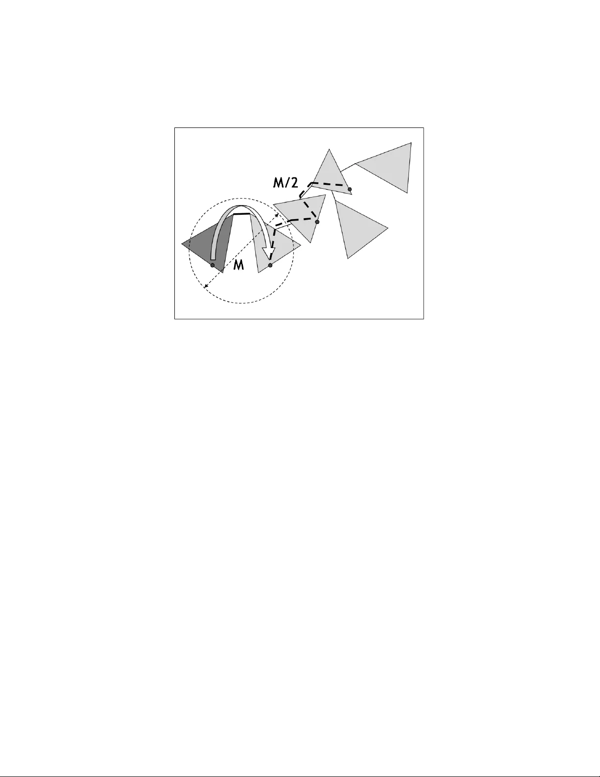
Ph ylogenies without Branc h Bounds: Con tracting the Short, Pruning the Deep Constan tinos Dask alakis Elc hanan Mossel ∗ Sebastien Roch Octob er 25, 2018 Abstract W e in tro duce a new phylogenetic reconstruction algorithm whic h, unlik e most previous rigorous inference techniques, does not rely on assumptions regarding the branc h lengths or the depth of the tree. The algorithm returns a forest whic h is guaran teed to con tain all edges that are: 1) sufficien tly long and 2) sufficien tly close to the lea ves. How m uch of the true tree is recov ered depends on the sequence length pro vided. The algorithm is distance-based and runs in polynomial time. 1 In tro duction In Ev olutionary Biology , the sp eciation history of a family of related or- ganisms is generally represen ted graphically by a phylo geny , that is, a tree where the lea ves are the observ ed (extan t) sp ecies and the branchings in- dicate sp eciation ev ents. T raditional approaches for reconstructing phy- logenies from homologous molecular sequences extracted from the observed sp ecies [F el04, SS03] are t ypically computationally in tractable [GF82, DS86, Da y87, CT06, Roc06], statistically inconsistent [F el78], or they require im- practical sequence lengths [Att99, LC06, SS99, SS02]. Nev ertheless, ov er the past decade, muc h progress has b een made in the design of efficien t, fast-con verging reconstruction techniques, starting with the seminal w ork of Erd¨ os et al. [ESSW99a]. The algorithm in [ESSW99a], often dubb ed the Short Quartet Metho d (SQM), is based on well-kno wn distance-matrix ∗ E.M. is supported by an Alfred Sloan fello wship in Mathematics and by NSF grants DMS-0528488, and DMS-0548249 (CAREER) and b y ONR gran t N0014-07-1-05-06. tec hniques, that is, it relies on estimates of the evolutionary distance be- t ween eac h pair of sp ecies (roughly the time elapsed since their most recent common ancestor). How ev er, unlik e other popular distance metho ds such as Neigh b or-Joining [SN87], the key b ehind SQM’s p erformance is that it discards long ev olutionary distances, whose estimates from sequence com- parisons are kno wn to b e statistically unreliable. The algorithm w orks b y first building subtrees of small diameter and, in a second stage, glueing the pieces bac k together. The Short Quartet Metho d is in fact guaran teed to return the correct top ology from p olynomial-length sequences in polynomial time with high probabilit y . But this app ealing theoretical performance comes at a price. The results of [ESSW99a] rely critically on biological assumptions which, although reasonable, are often not met in practice (see Section 1.3 for a formal statemen t): a) [Dense Sampling of Sp e cies] The observed sp ecies are “closely related.” In particular, there are no exceptionally long branches in the phy- logen y . b) [A bsenc e of Polytomies] The ph ylogeny is bifurcating. In fact, Erd¨ os et al. assume that sp eciation even ts are sufficien tly far apart to b e easily distinguished. The p oint of a) is that it implies a natural b ound on the depth of the tree whic h in turn ensures that enough information ab out the deep parts of the tree diffuses to the leav es. As for Assumption b), it guaran tees that a clear signal can b e extracted from eac h branc h of the phylogen y . It is ob vious—at least in tuitively—that assumptions such as a) and b) are necessary to secure the t yp e of results Erd¨ os et al. obtain: the guar ante e d r e c onstruction of the ful l phylo geny . Hence, to impro ve ov er SQM and obtain strong guaran tees under more general conditions, one has to relax this last requirement. In this paper, w e design an algorithm whic h provides strong reconstruc- tion guaran tees without Assumptions a) and b). W e sho w that our algorithm is guaranteed to reco ver a for est con taining all edges that are “sufficiently long” and “sufficien tly close” to the leav es. In fact, we allow a trade-off b et ween the resolution of short branches and the depth of the reconstructed forest, a feature of p otential practical in terest. Also, w e guaran tee that our reconstructed forest has the desirable prop ert y of being disjoint (although the presence of short edges leads us to allow deep intersections of v ery short branc hes b etw een the subtrees). Moreo v er, our algorithm do es not require the kno wledge of a priori b ounds on branc h lengths or tree depth. Finally 2 if Assumptions a) and b) are satisfied, we recov er the whole phylogen y and pro vide an alternativ e to the algorithm of Erd¨ os et al. Precise statements are giv en in Section 1.2. F or a full comparison to related w ork see also Section 1.3. 1.1 What can w e hop e to reconstruct? W ell-kno wn identifiabilit y results [Cha96] guarantee that phylogenies—or at least their idealized sto c hastic models—can b e fully reconstructed given enough data at the leav es. How ev er, molecular data gathered from current sp ecies are in essence limited, which begs the question: How much of the tr e e c an we r e al ly hop e to r e c onstruct? W e p ointed out ab o ve t w o imp ortan t sources of difficulties: short branc hes pro duce a weak signal that may be hard to detect; similarly , untangling the deep parts of the tree presents c hallenges that are well do cumen ted (see, e.g., [PL98, CDvM + 06]). Note that these issues are fundamen tally “information-theoretic” and affect all reconstruction metho ds. T o av oid these difficulties, most rigor ous metho ds imp ose restrictions on the length of the branc hes and/or the depth of the tree, whic h ma y b e unsatisfactory from a practical p ersp ective. On the other hand, metho ds commonly used in pr actic e , such as lik eliho o d and ba yesian methods, typ- ically pro duce sev eral candidate trees as well as confidence estimates. But theoretical guaran tees on the qualit y of suc h outputs are hard to obtain. Here, we seek to giv e strong reconstruction guarantees without any as- sumption on the true phylogen y . Our goal is to recov er, for an y given amoun t of data, as muc h of the tree as can rigorously be reconstructed with high confidence. Since the full ph ylogeny may not alw ays b e recov erable, w e are led to a more flexible solution concept: we output a c ontr acte d subfor est of the true ph ylogeny . That is, we output a forest con taining all branches that are “sufficiently long” and “sufficiently recen t”; note that “sufficien tly” here is determined (information-theoretically) b y the size of the data (usually in terms of sequence length). In the remainder of this section we formalize this solution concept. The input. F ormally , a ph ylogeny is a weighte d, multifur c ating tr e e on a set of leav es L , which w e iden tify with the lab els [ n ] = { 1 , . . . , n } . W e denote a ph ylogeny by T = ( V , E ; L, λ ). Here V and E are respectively the v ertex and edge set of the tree, and λ : E → (0 , + ∞ ) assigns a w eight to eac h edge (the branch length). W e assume that all internal vertices V − L ha ve degree at least 3. 3 Figure 1: The effect of distance distortion from the p ersp ective of a leaf. On the left hand side is the true phylogen y . On the right hand side, only distances within a certain radius represen t accurately the metric underlying the ph ylogeny . A ph ylogeny is naturally equipped with a so-called additive metric on the lea ves d : L × L → (0 , + ∞ ) defined as follo ws ∀ u, v ∈ L, d ( u, v ) = X e ∈ P T ( u,v ) λ e , where P T ( u, v ) is the set of edges on the path b et ween u and v in T . Often d ( u, v ) is referred to as the “ev olutionary distance” betw een sp ecies u and v . Since under the assumptions ab ov e there is a one-to-one corresp ondence b et ween d and λ , we write either T = ( V , E ; L, d ) or T = ( V , E ; L, λ ). W e also sometimes use the natural extension of d to the in ternal v ertices of T . W e denote by T the set of all ph ylogenies on an y num ber of leav es. It is well-kno wn that given an additive metric d one can reconstruct the corresp onding phylogen y T . How ev er, in practice, one can only derive an estimate ˆ d of d , the accuracy of whic h dep ends on the amoun t of data used. (This estimate is known in the literature as the “distance matrix”.) Our goal in this pap er is to reconstruct a ph ylogen y—or as m uch of it as p ossible—from this “distorted” version of its additive metric. A typical prop ert y of distance estimates is that estimates of long distances are unreli- able. The following definition formalizes this phenomenon. See Figure 1 for an illustration. Definition 1 (Distorted Metric [Mos07, KZZ03]) L et T = ( V , E ; L, d ) b e a phylo geny and let τ , M > 0 . We say that ˆ d : L × L → (0 , + ∞ ] is a ( τ , M ) - distorted metric for T or a ( τ , M ) - distortion of d if: 4 1. [Symmetry] F or al l u, v ∈ L , ˆ d is symmetric, that is, ˆ d ( u, v ) = ˆ d ( v , u ); 2. [Distortion] ˆ d is ac cur ate on “short” distanc es, that is, for al l u, v ∈ L , if either d ( u, v ) < M + τ or ˆ d ( u, v ) < M + τ then    d ( u, v ) − ˆ d ( u, v )    < τ . In ph ylogenetic reconstruction, a distorted metric is naturally deriv ed from samples of a Mark ov mo del on a tree—a common model of DNA sequence ev olution used in Biology . (See App endix A for details.) In the remainder of this pap er, w e assume that w e are given a ( τ , M )-distortion ˆ d of an additive metric d and we seek to recov er the underlying phylogen y T . Con traction and pruning. Given only a ( τ , M )-distorted metric, it is clear that the b est w e can hop e for in general is to reconstruct a forest con taining those edges of T that are “sufficien tly close” to the lea v es. In- deed, note that tw o phylogenies that are iden tical up to depth M from the lea ves, but are otherwise differen t, can giv e rise to the same distorted metric. Moreo ver, since w e do not assume that edges are longer than the accuracy τ , some edges may b e to o short to b e reconstructed and, as w e men tioned b efore, w e allo w ourselv es to instead contract them. Hence, w e are led to consider subforests of the true phylogen y where deep edges are prune d and short edges are c ontr acte d . T o formalize this idea w e need a few definitions. Let us first describ e what we mean by a subfor est of a phylogen y T = ( V , E ; L, d ). Giv en a set of vertices V 0 ⊆ V , the subtr e e of T r estricte d to V 0 is the tree obtained 1) b y keeping only no des and edges on paths b etw een vertices in V 0 and then 2) by con tracting all paths comp osed of v ertices of degree 2, except the no des in V 0 . See Figure 2 for an example. W e denote this tree b y T | V 0 . W e typically take V 0 ⊆ L . A subfor est of T is defined to b e a collection of restricted subtrees of T . W e also need a notion of depth. Giv en an edge e ∈ E , the chor d depth of e is the length of the shortest path among all paths crossing e betw een t wo leav es. That is, ∆ c ( e ) = min { d ( u, v ) : u, v ∈ L, e ∈ P T ( u, v ) } . W e define the chor d depth of a tr e e T to b e the maxim um chord depth in T ∆ c ( T ) = max { ∆ c ( e ) : e ∈ E } . 5 Figure 2: Restricting the top tree to its white no des. Definition 2 (Con tracted Subforest) L et T = ( V , E ; L, d ) b e a phylo geny. Fix M > 0 . L et { L 1 , . . . , L q } b e the natur al p artition of the le af set L ob- taine d by r emoving al l e dges e ∈ E such that ∆ c ( e ) ≥ M . We define the M - pruned subforest of T to b e the for est F M ( T ) = ( V M , E M ) c onsisting of the tr e es { T | L 1 , . . . , T | L q } . The metric d is extende d as fol lows for al l u, v ∈ L , d M ( u, v ) =  d ( u, v ) , if u, v are in the same subtree of F M ( T ) , + ∞ , o . w . We also denote by λ M the e dge lengths of F M ( T ) . Now, given also τ > 0 , the τ - contracted M - pruned subforest of T is the for est F τ ,M ( T ) = ( V τ ,M , E τ ,M ) obtaine d fr om F M ( T ) by c ontr acting e dges e ∈ E M of weight λ M ( e ) ≤ τ . P ath-disjoin tness. W e require that the trees of our reconstructed forest are “non-intersecting”. This is a natural condition to imp ose in order to obtain a meaningful reconstruction: w e wan t to av oid as muc h as p ossible that the same branc hes app ear in many subtrees. In fact, we can only guaran tee approximate disjointness as defined b elo w. W e first need a notion of depth for vertices. F or a ph ylogeny T = ( V , E ; L, d ) and a v ertex x ∈ V , the vertex depth of x is the length of the shortest path betw een x and the set of leav es. That is, ∆ v ( x ) = min { d ( u, x ) : u ∈ L } . 6 Giv en tw o lea ves u, v of T , w e denote b y e P T ( u, v ) the set of vertices on the path b et ween u and v in T . W e sa y that t wo trees are ( τ , M )-path disjoint if they are “almost dis- join t” in the sense that they only share edges (if an y) that are “deep” (end- p oin ts hav e vertex depth at least M / 2) and “short” (length at most τ ). More formally: Definition 3 (Appro ximate Path-Disjoin tness) L et T = ( V , E ; L, d ) b e a phylo geny. Two subtr e es T 1 , T 2 of T r estricte d r esp e ctively to L 1 , L 2 ⊆ L ar e ( τ , M )-path-disjoin t if L 1 ∩ L 2 = ∅ and for al l p airs of le aves u 1 , v 1 ∈ L 1 and u 2 , v 2 ∈ L 2 such that e P T ( u 1 , v 1 ) ∩ e P T ( u 2 , v 2 ) 6 = ∅ , we have: min { ∆ v ( x ) : x ∈ e P T ( u 1 , v 1 ) ∩ e P T ( u 2 , v 2 ) } ≥ 1 2 M , and, if further P T ( u 1 , v 1 ) ∩ P T ( u 2 , v 2 ) 6 = ∅ , max { λ e : e ∈ P T ( u 1 , v 1 ) ∩ P T ( u 2 , v 2 ) } ≤ τ . Mor e gener al ly, a c ol le ction of r estricte d subtr e es T 1 , . . . , T q of T ar e ( τ , M )- path-disjoin t if they ar e p airwise ( τ , M ) -p ath-disjoint. In the c ase τ = 0 , we simply say that the subtr e es ar e path-disjoint . 1.2 Main result and corollaries Main result. Our main result is an algorithm whic h, giv en a ( τ , M )- distorted metric, reconstructs a con tracted subforest (of the true ph ylogen y) whose trees are appro ximately path-disjoin t. T ypically , M is muc h larger than τ . In that case, w e reconstruct a subforest of T with c hord depth ≈ 1 2 M whic h includes all edges of length at least 4 τ . The reconstructed subtrees may “ov erlap” on edges of length at most 2 τ at v ertex depth ' 1 4 M . In Section 4, we show that these parameters are essentially optimal. The algorithm runs in p olynomial time. More precisely , we show: Theorem 1 (Main Result) L et τ and M b e monotone functions of n with M > 3 τ . L et m > 3 τ b e such that m < 1 2 [ M − 3 τ ] , 7 for al l n . Then, ther e is a p olynomial-time algorithm A such that, for al l phylo genies T = ( V , E ; L, d ) in T with | L | = n and al l ( τ , M ) -distortions ˆ d of d , A applie d to ˆ d satisfies the fol lowing: 1. [Appro ximate P ath Disjoin tness] A r eturns a (2 τ , m − 3 τ ) -p ath-disjoint subfor est b F of T ; 2. [Depth Guarantee] The for est b F is a r efinement of F 4 τ ,m − τ ( T ) ; W e give b elow a few imp ortan t sp ecial cases of Theorem 1. T ree case. When the amount of data is sufficient to pro duce a distorted metric with M = Ω(∆ c ( T )), we get a single comp onen t, that is, the full tree (up to those edges that are contracted). Corollary 1 (T ree Case) L et τ > 0 and M > 2∆ c ( T ) + 5 τ . Then, cho os- ing m > ∆ c ( T ) + τ guar ante es that the r e c onstructe d for est is c omp ose d of only a tr e e. In the case of “dense” phylogenies, M = Ω(log n ) is sufficient to reconstruct the full tree. Definition 4 (Dense Ph ylogenies (see e.g. [ESSW99a])) We say that a c ol le ction of phylo genies T 0 is dense if ther e is a 0 < g < + ∞ (indep endent of n ) such that for al l T = ( V , E ; L, λ ) ∈ T 0 we have ∀ e ∈ E , λ e ≤ g . (1) We denote by T g the set of phylo genies satisfying (1). Corollary 2 (Dense Case) In the c ase of dense phylo genies, M = Ω(log n ) suffic es to guar ante e the r e c onstruction of the ful l tr e e, up to c ontr acte d e dges. Absolute v arian t. All rigorous algorithms prior to our work (see Sec- tion 1.3) require kno wledge of either the tree depth or b ounds on the edge lengths to giv e strong reconstruction guarantees. This is not satisfactory from a practical p oin t of view. Here given only the sequence length we pro- vide explicit guarantees. The following result assumes that the distorted metric is deriv ed from a Marko v mo del on a tree. (See App endix A for details.) 8 Corollary 3 (Absolute V ariant) Given a numb er of samples k = Ω(log n ) fr om a Markov mo del on a tr e e and a chosen level of c ontr action ε > 0 (smal l), one c an cho ose τ , M , m so that A is guar ante e d to r eturn a (c on- tr acte d) subfor est of T c ontaining F ε,M 0 ( T ) with pr ob ability 1 − o (1) , wher e M 0 = Ω ε (log k − log log n ) . Complete resolution. Finally w e remark that, if we further assume that all branc h lengths are b ounded fr om b elow by a constant, then b y choosing τ accordingly a non-contracted forest is returned. In particular, we can reco ver the results of [ESSW99a]. 1.3 Related w ork Under a Mark o v model of ev olution, the Short Quartet Metho d (SQM) of Erd¨ os et al. [ESSW99a] is guaranteed to recov er the full ph ylogeny as long as the n um b er of samples k satisfies k > cf − 2 e c 0 g ∆ c ( T ) log n, for constants c, c 0 > 0, where f and g are resp ectiv ely low er and upp er b ounds on the branc h lengths p ossibly dep ending on n . F or instance, if f and g are constants the sequence length needed for complete reconstruction dep ends polynomially in the num ber of sp ecies. Mossel [Mos07] dev elop ed a framework that allo ws the reconstruction of a w ell-b ehav ed for est when sequences are to o short to guaran tee a complete reconstruction. More precisely , edges which are to o deep (in the sense of app earing only on paths b et ween sp ecies whose distances are not accurately kno wn) are prune d from the final reconstruction. A t a high level, Mossel’s Distorted Metric Metho d (DMM) (implicit in [Mos07]), works in a fashion similar to SQM—except for a pre-pro cessing phase that clusters together sufficien tly related sp ecies. Ho wev er, for DMM to work, lo wer bounds on the branc h lengths are required and, moreov er, these m ust b e known by the algorithm. F ollowing up on [Mos07], Dask alakis et al. [DHJ + 06] gav e a v ari- an t of DMM that runs without knowledge of a priori b ounds on the branc h lengths or the tree depth—making their v ariant somewhat more practical. Ho wev er, like DMM, the algorithm in [DHJ + 06] do es not deal prop erly with short edges: any part of the tree containing a short edge cannot b e recon- structed b y the algorithm (ev en though there may b e adjacen t edges that are in fact reconstructible). Therefore, in the presence of short edges no guaran tee can b e giv en ab out the depth of the reconstructed forest. 9 Exe cution Guar ante es No branc h Short edges Deep edges b ound needed OK OK [ESSW99a] [Mos07] X [DHJ + 06] X X [GMS08] X X Our metho d X X X Figure 3: Comparison of metho ds. Recen tly Gronau et al. [GMS08] eliminated the need for a low er b ound on the branch length b y c ontr acting edges whose length is b elow a user-defined threshold. Their solution uses a Directional Oracle (DO) whic h closes in on the lo cation of a leaf to b e added and, in the pro cess, con tracts regions that do not provide a reliable directional signal. Although the DO algorithm do es not use an explicit b ound on the depth of the tree, their r e c onstruction guar ante e requires such a b ound, similarly to [ESSW99a]. In particular, Gronau et al. lea ve op en the question of giving a forest-building version of their algorithm. Moreov er, the sequence length in [GMS08] depends exp o- nen tially on what the authors call the ε -diameter of the tree—essentially , the maxim um diameter of the con tracted regions. It is natural to conjecture that an optimal result should not dep end on this parameter. F or further related w ork on efficien t ph ylogeny reconstruction, see also [ESSW99b, HNW99, CK01, Csu02, KZZ03, MR06, DMR06]. 1.4 Discussion of the results In T able 3 w e summarize the curren t status as discussed in the previous sections. As the table emphasizes, our o verarc hing goal is to design an algorithm with go o d reconstruction guarantees in the presence of b oth short and deep edges, whose execution do es not rely on a priori b ounds on branch lengths. Unfortunately , giv en the com binatorial complexit y of Mossel’s forest-building algorithm, it is not straightforw ard to pro vide the extra flex- ibilit y of edge con traction in this framew ork. The nov elt y in our work is t wofold: • Solution Conc ept: A basic complication is that, in some sense, con- traction and pruning in terfere with eac h other. Indeed, the presence 10 of unresolv ed branc hes at the b oundary of partially reconstructed sub- trees creates the p ossibility of deep “undetectable” intersections. This pitfall seems to be una v oidable. One of our main contributions is to in- tro duce the notion of approximate disjoin tness, whic h allows short but deep in tersections b etw een subtrees of the reconstructed forest. This suitable solution concept leads to a quite simple algorithm with rea- sonable guaran tees. Moreov er, the flexibility in our definition allo ws us to reco v er all previously kno wn results as sp ecial cases. • A lgorithmic T e chnique: A natural approac h to forest building used in [Mos07, DHJ + 06] pro ceeds along the following three steps: 1. first, lea v es are group ed in to clusters for which all pairwise dis- tances are accurately known (the smal l clusters); 2. b y definition, the lo cal top ologies on the small clusters can b e trivially reconstructed [Bun71]; 3. finally , the lo cal top ologies that intersect in the true tree are “glued” together to get a forest (the resulting forest partitions the lea ves into lar ge clusters). This last step in volv es non-trivial combinatorial considerations. W e ha ve found that further allowing con tracted edges mak es this pro cess somewhat unmanageable. Instead w e use a different approach relying on simple metric arguments. In particular, we dir e ctly partition the lea ves into large clusters, whose underlying subtrees are appro ximately disjoin t, and provide a new straightforw ard metho d to reconstruct these subtrees. In addition, we obtain as sp ecial cases the results discussed in Section 1.3. In particular, if there are no short edges, we recov er the results of [Mos07] and [DHJ + 06], where a path-disjoin t forest is returned (b y taking τ equal to half the lo w er b ound on the branc h lengths in Theorem 1). If further- more there is an upp er bound on the branc h lengths, w e recov er the results of [ESSW99a] (Corollary 2). Finally , if w e k eep the upp er bound on the edge lengths, but drop the low er bound, w e reco v er the results of [GMS08] (Corol- lary 1). In fact, we eliminate the dep endence on the ε -diameter. 1 F urther, 1 After the results of the curren t pap er w ere p osted on the arXiv, we were informed b y S. Moran that, in parallel to our w ork, the authors of [GMS08] hav e impro ved on their previous results: the dep endence on the ε -diameter has b een remov ed. A preprint of this w ork is currently av ailable on the authors’ website. Note ho wev er that this new, indep endent work do es not deal with deep edges and still makes assumptions similar to [ESSW99a] restricting the depth of the generating tree. 11 unlik e [GMS08], we allow an arbitrary num b er of states, an extension—it should b e noted—that follows easily from [ESSW99b] and [Mos07]. 1.5 Organization The rest of the pap er is organized as follo ws. The algorithm is detailed in Section 2. The pro of of our main theorem follo ws in Section 3. W e conclude with a lo w er b ound in Section 4 and a discussion of the running time in Section 5. Also, for completeness, in App endix A we describ e the probabilistic motiv ation b ehind the distorted metric definition. The results in this pap er were announced without pro of in [DMR09]. Also, the coun ter-example in Section 4 did not app ear in [DMR09]. 2 Algorithm The outline of the algorithm follows. There are three main phases, which are explained in detail after the outline. The input to the algorithm is a ( τ , M )-distorted metric ˆ d on n leav es. In particular, we assume that the v alues τ and M are known to the algorithm (but see also Corollary 3). Let m b e as in Theorem 1. W e denote the true tree by T = ( V , E ; L, d ). The details of the subroutines Mini Contractor and Extender are detailed in Figures 5 and 7 (see also their high lev el description b elo w). • Pre-Pro cessing: Leaf Clustering. Build the distorted clustering graph b H m = ( b V m , b E m ) where b V m = [ n ] and ( u, v ) ∈ b E m ⇐ ⇒ ˆ d ( u, v ) < m ; compute the connected comp onents { ˆ h ( i ) m = ( ˆ v ( i ) m , ˆ e ( i ) m ) } q i =1 of b H m ; • Main Lo op. F or all comp onents i = 1 , . . . , q : – F or all pairs of lea ves u, v ∈ ˆ v ( i ) m suc h that ( u, v ) ∈ b E m : ∗ Mini Reconstruction. Compute { ψ j ( u, v ) } r ( u,v ) j =1 := Mini Contractor ( ˆ h ( i ) m ; u, v ); ∗ Bipartition Extension. Compute { ¯ ψ j ( u, v ) } r ( u,v ) j =1 := Extender ( ˆ h ( i ) m , { ψ j ( u, v ) } r ( u,v ) j =1 ; u, v ); – Deduce the tree b T ( i ) from { ¯ ψ j ( u, v ) } r ( u,v ) j =1 ; • Output. Return the resulting forest b F . 12 b Φ w u v w b Φ x − 1 ≥ 2 τ ? b B ( u, v ) Figure 4: Illustration of routine Mini Contractor . See Figure 5 for no- tation. Pre-pro cessing: Leaf clustering. As mentioned b efore, given a ( τ , M )- distortion we cannot hope to reconstruct edges that are to o deep inside the tree. This results in the reconstruction of a for est . Therefore, the first phase of the algorithm is to determine the “supp ort” of this forest. W e pro ceed as follo ws. Consider the follo wing graph on L . Definition 5 (Clustering Graph) L et M 0 ∈ [ τ , ≤ M − τ ] . The distorted clustering graph with parameter M 0 , denote d b H M 0 = ( b V M 0 , b E M 0 ) , is the fol lowing gr aph: the vertic es b V M 0 ar e the le aves L of T ; two le aves u, v ∈ L ar e c onne cte d by an e dge e = ( u, v ) ∈ b E M 0 if ˆ d ( u, v ) < M 0 . (2) Note that this is an undir e cte d gr aph b e c ause ˆ d is symmetric. Similarly, we define the clustering graph with parameter M 0 , H M 0 = ( V M 0 , E M 0 ) , wher e we use d inste ad ˆ d in (2). The first phase of the algorithm consists in building the graph b H m from ˆ d . W e then compute the connected comp onents of b H m whic h w e denote { ˆ h ( i ) m } q i =1 . In the next tw o phases, we build a tree on eac h of these comp o- nen ts. Building the comp onen ts I: Mini-reconstruction problem. Fix a comp onen t ˆ h ( i ) m of b H m . In this and the next phase, w e seek to reconstruct a contracted tree on ˆ h ( i ) m . Denote by T ( i ) the true tree T restricted to the lea ves in ˆ h ( i ) m . First, we find all edges of T ( i ) that are “sufficiently long” and lie on “sufficien tly short” paths. More precisely , w e consider all pairs 13 Algorithm Mini Contractor Input: Comp onen t ˆ h ( i ) m ; Lea ves u, v ; Output: Bipartitions { ψ j ( u, v ) } r ( u,v ) j =1 ; • Ball. Let b B ( u, v ) := n w ∈ ˆ v ( i ) m : ˆ d ( u, w ) ∨ ˆ d ( v , w ) < M o ; • In tersection P oints. F or all w ∈ b B ( u, v ), estimate the p oint of in tersection b etw een u, v , w (distance from u ), that is, b Φ w := 1 2  ˆ d ( u, v ) + ˆ d ( u, w ) − ˆ d ( v , w )  ; • Long Edges. Set S := b B ( u, v ) − { u } , x − 1 = u , j := 0, C 0 = { u } ; – Un til S = ∅ : ∗ Let x 0 = arg min { b Φ w : w ∈ S } (break ties arbitrarily); ∗ If b Φ x 0 − b Φ x − 1 ≥ 2 τ , create a new edge by setting ψ j +1 ( u, v ) := { b B ( u, v ) − S, S } and let C j +1 := { x 0 } , j := j + 1; ∗ Else, set C j := C j ∪ { x 0 } ; ∗ Set S := S − { x 0 } , x − 1 := x 0 ; • Output. Return the bipartitions { ψ j ( u, v ) } r ( u,v ) j =1 (where r ( u, v ) is the n umber of bipartitions generated in the previous step). Figure 5: Algorithm Mini Contractor . See Figure 4 for illustration. 14 of leav es u, v connected b y an edge in ˆ h ( i ) m , that is, lea ves within distorted distance m . F or each such pair u, v , the mini r e c onstruction pr oblem consists in finding all edges e in P T ( i ) ( u, v ) that hav e length larger than λ e ≥ 4 τ . T o do this using the distortion ˆ d , w e first consider a b al l b B ( u, v ) of all no des within distorted distance M of u and v , that is, b B ( u, v ) = n w ∈ ˆ h ( i ) m : ˆ d ( u, w ) ∨ ˆ d ( v , w ) < M o , where a ∨ b is the maximum of a and b . The p oin t of using this ball is that we can then guarantee that eac h edge in P T ( i ) ( u, v ) is “witnessed” b y a quartet (i.e., a 4-tuple of leav es) in b B ( u, v ) in the following sense: let ( x 1 , x 2 ) b e an edge in P T ( i ) ( u, v ) and let ( x j , y j ), j = 1 , 2, b e an edge adjacen t to x j that is not in P T ( i ) ( u, v ); for j = 1 , 2 let L ( i ) x j → y j b e the lea ves reac hable from y j using paths not including x j ; then we will show that L ( i ) x j → y j ∩ b B ( u, v ) 6 = ∅ for j = 1 , 2. In other words, there is enough information in b B ( u, v ) to reconstruct all edges in P T ( i ) ( u, v )—at least those that are “sufficien tly long.” This phase is detailed in Figure 5. An illustration is giv en in Figure 4. Building the comp onen ts I I: Extending the bipartitions. The pre- vious step reconstructs “sufficien tly long” edges on balls of the form b B ( u, v ). By r e c onstructing an e dge on b B ( u, v ), w e mean finding the bip artition of b B ( u, v ) to which the e dge c orr esp onds . More precisely: Definition 6 (Bipartitions) L et T = ( V , E ) b e a multifur c ating tr e e with no vertex of de gr e e 2 . Each e dge e in T induc es a bipartition of the le aves L of T as fol lows: if one r emoves the e dge e fr om T , then one is left with two c onne cte d c omp onents; take the p artition of the le aves c orr esp onding to those c omp onents. Denote by b T ( e ) the bip artition of e on T . It is e asy to se e that given the bip artitions { b T ( e ) } e ∈ E one c an r e c onstruct the tr e e T efficiently [Bun71, Me a81, BD86]. (Pr o c e e d by se quential ly “splitting” clusters.) The goal of the second phase in the main loop of our reconstruction algo- rithm is to extend the bipartitions previously built from b B ( u, v ) to the full comp onen t ˆ h ( i ) m . T o p erform this task, we use the follo wing observ ation: supp ose w e w ant to deduce the bipartition corresp onding to edge e ; since the radius of the ball b B ( u, v ) is m uch larger than m , we can mak e sure that a path fr om a leaf in ˆ h ( i ) m that is outside b B ( u, v ) to a leaf on the other side of the bipartition b T ( e ) is “long.” Therefore, we can easily determine what 15 Figure 6: Illustration of routine Extender . See also Figure 7. side of the partition eac h leaf in ˆ h ( i ) m lies on. F or details, see Figure 7. An illustration is giv en in Figure 6. 3 Analysis of the Algorithm W e assume throughout that ˆ d is a ( τ , M )-distortion of d and moreo ver that m satisfies the conditions of Theorem 1. 3.1 Leaf clustering: Determining the supp ort of the forest Recall the notation of Definition 5. Prop osition 1 (Leaf Clustering) L et τ ≤ M 0 ≤ M − τ . Then E M 0 − τ ⊆ b E M 0 ⊆ E M 0 + τ . Pro of: This follows immediately from the definition of ˆ d . Indeed, if d ( u, v ) < M 0 − τ then ˆ d ( u, v ) < d ( u, v ) + τ < ( M 0 − τ ) + τ < M 0 . Similarly , if ˆ d ( u, v ) < M 0 then d ( u, v ) < ˆ d ( u, v ) + τ < M 0 + τ . 16 Algorithm Extender Input: Comp onen t ˆ h ( i ) m ; Bipartitions { ψ j ( u, v ) } r ( u,v ) j =1 ; Lea ves u, v ; Output: Bipartitions { ¯ ψ j ( u, v ) } r ( u,v ) j =1 ; • F or j = 1 , . . . , r ( u, v ) (unless r ( u, v ) = 0): – Initialization. Denote by ψ ( u ) j ( u, v ) the vertex set con taining u in the bipartition ψ j ( u, v ), and similarly for v ; Initialize the ex- tended partition ¯ ψ ( u ) j ( u, v ) := ψ ( u ) j ( u, v ), ¯ ψ ( v ) j ( u, v ) := ψ ( v ) j ( u, v ); – Mo dified Graph. Let K be ˆ h ( i ) m where all edges b et ween ψ ( u ) j ( u, v ) and ψ ( v ) j ( u, v ) hav e been remov ed; – Extension. F or all w ∈ ˆ v ( i ) m − ( ψ ( u ) j ( u, v ) ∪ ψ ( v ) j ( u, v )), add w to the side of the partition it is connected to in K (by Proposition 6, eac h w as ab ov e is connected to exactly one side); • Return the bipartitions { ¯ ψ j ( u, v ) } r ( u,v ) j =1 . Figure 7: Algorithm Extender . See Figure 6 for an illustration.  3.2 Mini-reconstruction: Finding long edges on short paths Consider a comp onen t ˆ h ( i ) m = ( ˆ v ( i ) m , ˆ e ( i ) m ) of b H m . Denote by T ( i ) = ( V ( i ) , E ( i ) ) the tree T restricted to the lea ves in ˆ v ( i ) m , that is, • Keep only those edges of T that are on paths b etw een lea ves in ˆ v ( i ) m ; • Glue together edges adjacent to vertices of degree 2; • Equip T ( i ) with the metric d restricted to ˆ v ( i ) m × ˆ v ( i ) m and denote { λ ( i ) e } e ∈ E ( i ) the corresp onding weigh ts. Prop osition 2 (Chord Depth of T ( i ) ) The chor d depth of T ( i ) is less than m + τ . Pro of: W e argue b y contradiction. Let e be an edge in T ( i ) . Supp ose that the chord depth of e in T ( i ) is ≥ m + τ . Consider the bipartition { ψ (1) , ψ (2) } defined by e in T ( i ) . Then it follo ws that for all u 1 ∈ ψ (1) and u 2 ∈ ψ (2) , we ha ve ˆ d ( u 1 , u 2 ) > d ( u 1 , u 2 ) − τ ≥ m, 17 so that ˆ h ( i ) m cannot b e connected, a contradiction.  Let e 0 = ( u 0 , v 0 ) be an edge in a tree T 0 with leaf set L 0 . W e denote by L 0 u 0 → v 0 the leav es of T 0 that can b e reac hed from v 0 without going through u 0 . Recall that for tw o leav es u 0 , v 0 of T 0 , we denote b y e P T 0 ( u 0 , v 0 ) the set of v ertices on the path betw een u 0 and v 0 in T 0 . Recall also that b B ( u, v ) = n w ∈ ˆ v ( i ) m : ˆ d ( u, w ) ∨ ˆ d ( v , w ) < M o , for u, v ∈ ˆ v ( i ) m . Prop osition 3 (Witnesses in b B ( u, v ) ) Assume that 2 m + 3 τ < M . L et ( u, v ) ∈ ˆ e ( i ) m . L et ( x, y ) b e an e dge of T ( i ) such that x ∈ e P T ( i ) ( u, v ) but y / ∈ e P T ( i ) ( u, v ) . Then we have b B ( u, v ) ∩ L ( i ) x → y 6 = ∅ , wher e L ( i ) is the set of le aves of T ( i ) . Pro of: By Prop osition 2, there are lea v es x 0 , y 0 in L ( i ) suc h that ( x, y ) ∈ P T ( i ) ( x 0 , y 0 ) and d ( x 0 , y 0 ) < m + τ . Assume without loss of generality that y 0 ∈ L ( i ) x → y . By assumption, d ( u, v ) < ˆ d ( u, v ) + τ < m + τ . Therefore, d ( u, y 0 ) ≤ d ( u, x ) + d ( x, y 0 ) ≤ d ( u, v ) + d ( x 0 , y 0 ) < 2 m + 2 τ , from whic h we get ˆ d ( u, y 0 ) < 2 m + 3 τ < M . The same inequality holds for ˆ d ( v , y 0 ).  Fix a pair of leav es u, v with ( u, v ) ∈ ˆ e ( i ) m . F or w ∈ b B ( u, v ), let b Φ w := 1 2  ˆ d ( u, v ) + ˆ d ( u, w ) − ˆ d ( v , w )  , and Φ w := 1 2 ( d ( u, v ) + d ( u, w ) − d ( v , w )) . Note that Φ w is the distance b et ween u and the int ersection p oint of { u, v , w } . Let { C j } r ( u,v ) j =0 and { ψ j ( u, v ) } r ( u,v ) j =1 b e as in Figure 5. W e write w ∼ w 0 if w , w 0 ∈ C j for some j . Similarly , w e write w . w 0 (resp ectiv ely w < w 0 ) if w ∈ C j and w 0 ∈ C j 0 with j ≤ j 0 (resp ectiv ely j < j 0 ). 18 Prop osition 4 (In tersection Poin ts) L et u, v b e as ab ove. Then we have the fol lowing: 1. [Iden tity] If x, y ∈ b B ( u, v ) ar e such that Φ x = Φ y then x ∼ y ; 2. [Precedence] If x, y ∈ b B ( u, v ) ar e such that Φ x ≤ Φ y then x . y ; 3. [Separation] If x, y ∈ b B ( u, v ) ar e such that Φ x < Φ y − 4 τ and ther e is no z ∈ b B ( u, v ) with Φ x < Φ z < Φ y , then x < y . Pro of: F or P art 1, note that Φ x = Φ y implies    b Φ x − b Φ y    < 2 τ . (Note that the term ˆ d ( u, v ) app ears in b oth b Φ x and b Φ y and therefore do es not con tribute to the error. The same argument applies to the error calculations b elo w.) Therefore, x and y are necessarily placed in the same C j , that is, x ∼ y . See Figure 5. F or Part 2, suppose by con tradiction that x > y . Then we hav e neces- sarily b Φ x ≥ b Φ y + 2 τ , whic h implies Φ y < Φ x − 2 τ + 2 τ ≤ Φ x , a con tradiction. F or Part 3, let X 0 = { w ∈ b B ( u, v ) s . t . Φ w ≤ Φ x } , Y 0 = { w ∈ b B ( u, v ) s . t . Φ w ≥ Φ y } , x 0 = arg max { b Φ w : w ∈ X 0 } , (breaking ties arbitrarily) and similarly y 0 = arg min { b Φ w : w ∈ Y 0 } . Note that by assumption the pair X 0 , Y 0 forms a partition of b B ( u, v ). By assumption, Φ x 0 ≤ Φ x < Φ y − 4 τ ≤ Φ y 0 − 4 τ , whic h implies for all x 0 ∈ X 0 and y 0 ∈ Y 0 b Φ y 0 ≥ b Φ y 0 > b Φ x 0 + 4 τ − 2 τ ≥ b Φ x 0 + 2 τ ≥ b Φ x 0 + 2 τ . Therefore, w e ha ve x < y .  19 Prop osition 5 (Mini Reconstruction) L et u, v b e as ab ove. Assume that 2 m + 3 τ < M . Then we have the fol lowing: 1. [Reconstructed Edges Are Correct] F or e ach j = 1 , . . . , r ( u, v ) , ther e is a unique e dge e in E ( i ) such that b T ( i ) ( e ) ∩ b B ( u, v ) = ψ j ( u, v ) , wher e the interse ction on the left is applie d sep ar ately to e ach set in the p artition; 2. [Long Edges Are Present] L et e ∈ E ( i ) with e ∈ P T ( i ) ( u, v ) and λ ( i ) e > 4 τ . Then ther e is a unique j such that b T ( i ) ( e ) ∩ b B ( u, v ) = ψ j ( u, v ) . Pro of: Part 1 follows from Prop osition 3 and Prop osition 4 P art 2. Indeed, b y Prop osition 4 Part 2, ψ j ( u, v ) is a correct bipartition of T ( i ) restricted to b B ( u, v ). It corresponds to a unique edge of the latter tree because it is a full bipartition of b B ( u, v ). By Prop osition 3, every edge of T ( i ) is witnessed in b B ( u, v ), so ψ j ( u, v ) must also corresp ond to a unique edge in T ( i ) . Similarly , Part 2 follows from Proposition 3 and Proposition 4 Parts 2 and 3.  3.3 Extending bipartitions: Reconstructing the comp onents Let u, v ∈ ˆ v ( i ) m with ( u, v ) ∈ ˆ e ( i ) m and let ψ j ( u, v ) b e one of the bipartitions returned b y Mini Contractor when given ( ˆ h ( i ) m ; u, v ) as input. Let e = ( x, y ) ∈ E ( i ) b e the edge of T ( i ) corresp onding to ψ j ( u, v ) (as guaranteed by Prop osition 5) and denote its bipartition b y b T ( i ) ( e ) = { b ( u ) , b ( v ) } , where b ( u ) and b ( v ) are resp ectiv ely the sides con taining u and v . Prop osition 6 (Lea v es Outside Ball) Assume that 2 m + 3 τ < M . L et w ∈ ˆ v ( i ) m − b B ( u, v ) . Assume that w ∈ b ( v ) . Then, for al l le aves w 0 in b ( u ) we have ˆ d ( w , w 0 ) ≥ m. 20 Pro of: Assume b y con tradiction that there is w 0 ∈ b ( u ) suc h that ˆ d ( w , w 0 ) < m . The path betw een w and w 0 m ust go through e since w and w 0 are on differen t sides of the partition. Therefore, for one of the endp oints of e , sa y x , w e hav e d ( w , x ) < m + τ . Also, since d ( u, x ) ≤ d ( u, v ) < ˆ d ( u, v ) + τ < m + τ , w e hav e d ( w , u ) < d ( w , x ) + d ( x, u ) < 2 m + 2 τ < M . W e finally get ˆ d ( w , u ) < d ( w , u ) + τ < 2 m + 3 τ < M , and similarly for ˆ d ( w , v ), a contradiction since we assumed w / ∈ b B ( u, v ).  Prop osition 7 (Correct Extension) The bip artition ¯ ψ j ( u, v ) r eturne d by Extender is c orr e ct, that is, ¯ ψ j ( u, v ) = b T ( i ) ( e ) . Pro of: Let K , ψ ( u ) j ( u, v ), ψ ( v ) j ( u, v ) be as in Figure 7. Since ˆ h ( i ) m is connected and w e only remov e edges b etw een ψ ( u ) j ( u, v ) and ψ ( v ) j ( u, v ) to form K , it follo ws from Prop osition 6 that all vertices in ˆ v ( i ) m − ( ψ ( u ) j ( u, v ) ∪ ψ ( v ) j ( u, v )) are connected in K to either ψ ( u ) j ( u, v ) or ψ ( v ) j ( u, v ).  W e finally get the follo wing. Prop osition 8 (Correctness of Main Lo op) L et { b T ( i ) } q i =1 b e the tr e es obtaine d at the end of the Main L o op of our algorithm. Then, for al l i = 1 , . . . , q , b T ( i ) is a r efinement of F 4 τ , + ∞ ( T ( i ) ) . Pro of: By Prop ositions 5 and 7, all reconstructed edges are correct and they include at least those edges longer than 4 τ .  3.4 P ath-disjoin tness: Length and depth of shared edges Let T ( i 1 ) , T ( i 2 ) b e the tree T restricted to comp onents ˆ h ( i 1 ) m , ˆ h ( i 2 ) m resp ectiv ely . Note that eac h edge in T ( i j ) is actually a path in T . Prop osition 9 (P ath-Disjoin tness) F or al l u 1 , v 1 ∈ L ( i 1 ) and u 2 , v 2 ∈ L ( i 2 ) such that e P T ( u 1 , v 1 ) ∩ e P T ( u 2 , v 2 ) 6 = ∅ , it holds that 21 1. [Depth of Shared V ertices] We have min { ∆ v ( z ) : z ∈ e P T ( u 1 , v 1 ) ∩ e P T ( u 2 , v 2 ) } ≥ 1 2 ( m − 3 τ ) . 2. [Length of Shared Edges] If, further, P T ( u 1 , v 1 ) ∩ P T ( u 2 , v 2 ) 6 = ∅ then max { λ e : e ∈ P T ( u 1 , v 1 ) ∩ P T ( u 2 , v 2 ) } ≤ 2 τ . Pro of: Let z ∈ e P T ( u 1 , v 1 ) ∩ e P T ( u 2 , v 2 ). F or j = 1 , 2, by Proposition 2, there are lea ves x j , y j in L ( i j ) suc h that z ∈ e P T ( i j ) ( x j , y j ) and d ( x j , y j ) < m + τ . F or P art 1, assume without loss of generality that d ( x 2 , z ) < 1 2 ( m + τ ). Then, for all w ∈ L ( i 1 ) , d ( w , z ) ≥ d ( w , x 2 ) − d ( z , x 2 ) ≥ m − τ − 1 2 ( m + τ ) ≥ 1 2 ( m − 3 τ ) . A similar argumen t applies to w ∈ L ( i 2 ) and w ∈ L − ( L ( i 1 ) ∪ L ( i 2 ) ). F or Part 2, let e = ( x, y ) ∈ P T ( u 1 , v 1 ) ∩ P T ( u 2 , v 2 ). Assume without loss of generality that the path from x to y partitions { x 1 , y 1 , x 2 , y 2 } as {{ x 1 , x 2 } , { y 1 , y 2 }} in T , where x 1 , x 2 , y 1 , y 2 w ere defined ab o ve. W e hav e 2 d ( x, y ) = d ( x 1 , y 1 ) + d ( x 2 , y 2 ) − d ( x 1 , x 2 ) − d ( y 1 , y 2 ) < ˆ d ( x 1 , y 1 ) + ˆ d ( x 2 , y 2 ) − ˆ d ( x 1 , x 2 ) − ˆ d ( y 1 , y 2 ) + 4 τ < 2 m − 2 m + 4 τ < 4 τ , where the third line follo ws from the definition of the clustering graph b H m .  3.5 Pro of of Main Theorem Pro of of Theorem 1: Part 1 follows from Prop osition 9. Recall that m < 1 2 [ M − 3 τ ] . P art 2 then follo ws from Prop osition 8 and Prop osition 1.  22 Figure 8: Counter-example: Reference tree T 0 . 4 Tigh tness of the Result W e show ed that giv en a ( τ , M )-distortion w e reconstruct a subforest of T with chord depth ≈ 1 2 M which includes all edges of length at least 4 τ . It ma y seem that w e are losing a factor 2 in the chord depth and that, in fact, w e should b e able to reconstruct edges of chord depth close to M . But this is not the case. W e show in this section that the chord depth of ≈ 1 2 M is essen tially b est p ossible (up to O ( τ )). Consider the tree T 0 depicted in Figure 8. The tree T 0 has four lea v es u, v , x 1 , x 2 with adjacent edges of length resp ectively 4 τ , 1 2 M + 2 τ , 1 2 M + 4 τ , and 1 2 M + 4 τ . The middle edge has length 4 τ and the corresponding bipartition is {{ u, x 1 } , { v , x 2 }} . Assume that w e hav e the following ( τ , M )- distortion of the metric corresp onding to T 0 : ˆ d 0 ( u, v ) = 1 2 M + 10 τ , ˆ d 0 ( u, x 1 ) = 1 2 M + 8 τ , ˆ d 0 ( u, x 2 ) = 1 2 M + 12 τ , ˆ d 0 ( v , x 1 ) = ˆ d 0 ( v , x 2 ) = ˆ d 0 ( x 1 , x 2 ) = + ∞ . No w, note that ˆ d 0 is also a ( τ , M )-distortion for the tree T 1 depicted 23 Figure 9: Counter-example: T ree T 1 with equiv alent distortion. in Figure 9. The tree T 1 has four leav es u, v , x 1 , x 2 with adjacent edges of length resp ectiv ely 4 τ , 1 2 M + 2 τ , 1 2 M , and 1 2 M + 8 τ . The middle e dge has length 4 τ and the corresp onding bipartition is {{ u, x 2 } , { v , x 1 }} . Hence, the t wo incompatible trees T 0 and T 1 cannot in general b e distin- guished from a ( τ , M )-distortion. In particular, note that the middle edge of T 0 has length 4 τ and c hord depth 1 2 M + 10 τ , y et its bipartition cannot b e reco vered. This prov es the c laim. 5 Implemen tation W e briefly discuss the running time of the algorithm. Building the graph b H m tak es time O ( n 2 ), since w e hav e to consider all pairs of lea ves, and we find the connected comp onen ts of b H m with Breadth- First-Searc h in another O ( n 2 ). W e argue next that, for i = 1 , . . . , q , we need O ( n 5 i ) to build b T ( i ) , where n i = | ˆ v ( i ) m | . W e show first that for all pairs of leav es u and v , Mini Contra ctor and Extender take time O ( n 3 i ). Indeed, Mini Contractor takes time O ( n i ), since its running time is 24 linear in the size of b B ( u, v ); and Extender takes time O ( n 3 i ), since for eac h bipartition ψ j ( u, v )—there are at most O ( n i ) of those—it is enough to p erform a BFS. Giv en all bipartitions of the tree b T ( i ) , we use the standard TREE POPPING algorithm of [Mea81, BD86] to build b T ( i ) ; since we ha ve O ( n 3 i ) bipartitions (not all of them distinct) this last step takes time O ( n 4 i ). So for eac h tree i w e need O ( n 5 i ), and summing o ver i ’s the total running time b ecomes O ( n 5 ). W e can improv e on this running time by a more efficien t implemen tation of Extender as follows. F or all j = 0 , . . . , r ( u, v ), w e remov e from the graph ˆ h ( i ) m all lea ves in ∪ ` 6 = j C ` and p erform a Breadth-First-Search to discov er the lea ves K j ⊂ ˆ v ( i ) m \ b B ( u, v ) reachable in ˆ h ( i ) m from the leav es in C j . F rom an easy mo dification of Prop ositions 5 ans 6, it follows that for every w / ∈ b B ( u, v ) there is at most one j ∈ { 0 , . . . , r ( u, v ) } suc h that w is connected to a leaf in C j . Given this, we can argue that w e can reco ver the bipartitions ¯ ψ j ( u, v ), j = 1 , . . . , r ( u, v ) from the K j ’s. The ov erall time needed b y the BFS’s is O ( n 2 i ), hence b T ( i ) can b e computed in time O ( n 4 i ) and our total running time b ecomes O ( n 4 ). The ab o ve implemen tation is wasteful in running a BFS for every pair of lea ves u and v with the p ossibilit y of creating as man y as O ( n 3 ) bipartitions, eac h requiring O ( n ) storage. Note that there are in fact at most n distinct bipartitions in T . T o improv e on the running time one may need to com bine the BFS’s performed in the ab o ve implementation by interlea ving the Mini Contractor and Extender steps with the TREE POPPING algorithm. 6 Concluding remarks An interesting question for future work is whether the appr oximate disjoin t- ness in our results can b e av oided. Since we guarantee that an y shared edge lies deep inside the forest, it is tempting to simply remov e all deep edges (sa y b eyond m/ 4) from the output forest. Unfortunately , man y of these edges may in fact b e contracted and moreov er they may b e clustered in “su- p erno des” including b oth dee p and not-so-deep edges. It do es not seem to b e a trivial task to break these deep sup erno des apart and preserve strong reconstruction guaran tees. 25 References [A tt99] K. Atteson. The p erformance of neigh b or-joining metho ds of ph ylogenetic reconstruction. Algorithmic a , 25(2-3):251–278, 1999. [BD86] Hans-J ¨ urgen Bandelt and Andreas Dress. Reconstructing the shap e of a tree from observed dissimilarit y data. A dv. in Appl. Math. , 7(3):309–343, 1986. [BH87] Daniel Barry and J. A. Hartigan. Statistical analysis of homi- noid molecular evolution. Statist. Sci. , 2(2):191–210, 1987. With comments by Stephen Portno y and Joseph F elsenstein and a reply by the authors. [Bun71] P . Buneman. The recov ery of trees from measures of dissimi- larit y . In Mathematics in the Ar chaelo gic al and Historic al Sci- enc es , pages 187–395. Edinburgh Universit y Press, Edin burgh, 1971. [CDvM + 06] F rancesca D. Ciccarelli, T obias Do erks, Christian von Mering, Christopher J. Creevey , Berend Snel, and P eer Bork. T ow ard Automatic Reconstruction of a Highly Resolved T ree of Life. Scienc e , 311(5765):1283–1287, 2006. [Cha96] Joseph T. Chang. F ull reconstruction of Mark ov mo dels on ev o- lutionary trees: identifiabilit y and consistency . Math. Biosci. , 137(1):51–73, 1996. [CK01] Mikl´ os Csur¨ os and Ming-Y ang Kao. Prov ably fast and accurate reco very of ev olutionary trees through harmonic greedy triplets. SIAM Journal on Computing , 31(1):306–322, 2001. [Csu02] M. Csur¨ os. F ast recov ery of ev olutionary trees with thousands of no des. J. Comput. Biol. , 9(2):277–97, 2002. [CT06] Benny Chor and T amir T uller. Finding a maxim um likelihoo d tree is hard. J. A CM , 53(5):722–744, 2006. [Da y87] William H. E. Day . Computational complexit y of inferring ph ylogenies from dissimilarity matrices. Bul l. Math. Biol. , 49(4):461–467, 1987. 26 [DHJ + 06] Constan tinos Dask alakis, Cameron Hill, Alexander Jaffe, Radu Mihaescu, Elc hanan Mossel, and Satish Rao. Maximal accurate forests from distance matrices. In RECOMB , pages 281–295, 2006. [DMR06] Constan tinos Dask alakis, Elc hanan Mossel, and S´ ebastien Ro c h. Optimal phylogenetic reconstruction. In STOC’06: Pr o- c e e dings of the 38th Annual ACM Symp osium on The ory of Computing , pages 159–168, New Y ork, 2006. A CM. [DMR09] Constan tinos Dask alakis, Elc hanan Mossel, and S´ ebastien Ro c h. Ph ylogenies without branch b ounds: Con tracting the short, pruning the deep. T o app ear in RECOMB 2009, 2009. [DS86] William H. E. Da y and Da vid Sankoff. Computational com- plexit y of inferring phylogenies b y compatibilit y . Syst. Zo ol. , 35(2):224–229, 1986. [ESSW99a] P . L. Erd¨ os, M. A. Steel, L. A. Sz´ ekely , and T. A. W arnow. A few logs suffice to build (almost) all trees (part 1). R andom Struct. Algor. , 14(2):153–184, 1999. [ESSW99b] P . L. Erd¨ os, M. A. Steel, L. A. Sz´ ekely , and T. A. W arnow. A few logs suffice to build (almost) all trees (part 2). The or. Comput. Sci. , 221:77–118, 1999. [F el78] J. F elsenstein. Cases in which parsimony or compatibilit y meth- o ds will be p ositively misleading. Syst. Biol. , pages 401–410, 1978. [F el04] J. F elsenstein. Inferring Phylo genies . Sinauer, Sunderland, MA, 2004. [GF82] R. L. Graham. and L. R. F oulds. Unlik eliho o d that minimal ph ylogenies for a realistic biological study can b e constructed in reasonable computational time. Math. Biosci. , 60:133–142, 1982. [GMS08] Ilan Gronau, Shlomo Moran, and Sagi Snir. F ast and reliable reconstruction of phylogenetic trees with very short edges. T o app ear in SODA, 2008. 27 [HNW99] D. H. Huson, S. H. Nettles, and T. J. W arnow. Disk-cov ering, a fast-con verging method for ph ylogenetic tree reconstruction. J. Comput. Biol. , 6(3–4), 1999. [KZZ03] V alerie King, Li Zhang, and Y unhong Zhou. On the complexit y of distance-based evolutionary tree reconstruction. In SODA ’03: Pr o c e e dings of the fourte enth annual ACM-SIAM symp o- sium on Discr ete algorithms , pages 444–453, Philadelphia, P A, USA, 2003. Society for Industrial and Applied Mathematics. [Lak94] JA Lak e. Reconstructing Evolutionary T rees from DNA and Protein Sequences: P aralinear Distances. Pr o c e e dings of the National A c ademy of Scienc es , 91(4):1455–1459, 1994. [LC06] Mic helle R. Lacey and Joseph T. Chang. A signal-to-noise anal- ysis of phylogen y estimation b y neighbor-joining: insufficiency of polynomial length sequences. Math. Biosci. , 199(2):188–215, 2006. [LSHP94] PJ Lo ckhart, MA Steel, MD Hendy , and D Penn y . Recov ering Ev olutionary T rees under a More Realistic Mo del of Sequence. Mol Biol Evol , 11(4):605–612, 1994. [Mea81] C. A. Meacham. A manual metho d for character compatibilit y analysis. T axon , 30:591–600, 1981. [Mos07] E. Mossel. Distorted metrics on trees and ph ylogenetic forests. IEEE/A CM T r ans. Comput. Bio. Bioinform. , 4(1):108–116, 2007. [MR06] Elchanan Mossel and S´ ebastien Ro ch. Learning nonsingular ph ylogenies and hidden Mark o v mo dels. A nn. Appl. Pr ob ab. , 16(2):583–614, 2006. [PL98] H. Philippe and J. Laurent. Ho w goo d are deep phylogenetic trees? Curr ent Opinion in Genetics & Development , 8:616– 623(8), Decem b er 1998. [Ro c06] S ´ ebastien Ro c h. A short pro of that phylogenetic tree recon- struction b y maxim um likelihoo d is hard. IEEE/ACM T r ans. Comput. Biolo gy Bioinform. , 3(1):92–94, 2006. 28 [SN87] N. Saitou and M. Nei. The neighbor-joining metho d: A new metho d for reconstructing phylogenetic trees. Mol. Biol. Evol. , 4(4):406–425, 1987. [SS99] Mic hael A. Steel and L´ aszl´ o A. Sz ´ ek ely . Inv erting random func- tions. Ann. Comb. , 3(1):103–113, 1999. Combinatorics and biology (Los Alamos, NM, 1998). [SS02] M. A. Steel and L. A. Sz´ ekely . Inv erting random functions. I I. Explicit b ounds for discrete maximum likelihoo d estima- tion, with applications. SIAM J. Discr ete Math. , 15(4):562–575 (electronic), 2002. [SS03] C. Semple and M. Steel. Phylo genetics , volume 22 of Math- ematics and its Applic ations series . Oxford Univ ersity Press, 2003. [Ste94] M. Steel. Recov ering a tree from the leaf colourations it gen- erates under a Mark ov mo del. Appl. Math. L ett. , 7(2):19–23, 1994. 29 A Log-Det Estimator F or completeness, w e relate the definition of the distorted metric (see Defini- tion 1) to its biological context. In phylogenetic reconstruction, a distorted metric is naturally deriv ed from samples of a Marko v mo del on a tree—a common mo del of DNA sequence evolution used in Biology . Definition 7 (Mark o v model on a tree) A Marko v mo del on a tree is the fol lowing sto chastic pr o c ess: • L et T ρ = ( V , E , ρ ) b e a finite tr e e r o ote d at ρ . Denote by E ↓ the set E dir e cte d away fr om the r o ot. • L et L = [ n ] b e the le af set of T ρ . • L et R b e a finite set with r elements. • Asso ciate to e ach e dge e ∈ E a r × r sto chastic matrix M ( e ) with det M ( e ) > 0 . • L et π ρ b e a distribution on R with π ρ ( σ ) > 0 for al l σ ∈ R . The pr o c ess runs as fol lows. Pick a state for the r o ot ac c or ding to π ρ . Moving away fr om the r o ot towar d the le aves, apply the channel M ( e ) to e ach e dge e indep endently. Denote the state so obtaine d σ V = ( σ v ) v ∈ V . In p articular, σ [ n ] is the state at the le aves. Mor e pr e cisely, the joint distribution of σ V is given by µ V ( σ V ) = π ρ ( σ ρ ) Y e =( x,y ) ∈ E ↓ ( M ( e )) σ x σ y , and ther efor e the distribution at the le aves is µ L ( σ L ) = X σ 0 V : σ 0 L = σ L π ρ ( σ 0 ρ ) Y e =( x,y ) ∈ E ↓ ( M ( e )) σ 0 x σ 0 y . F or W ⊆ V , we denote by µ W the mar ginal of µ V at W . More generally , we are giv en k indep enden t samples ( σ i [ n ] ) k i =1 from the same Mark ov mo del. W e think of ( σ i l ) k i =1 as the sequence at l ∈ [ n ]. Typically in biological applications R = { A , G , C , T } . MMTs mo del how DNA sequences sto c hastically evolv e by p oint mutations along an evolutionary tree—under the assumption that each site in the sequences ev olves indep endently . 30 In the phylogenetic reconstruction problem, w e are given sequences ( σ i [ n ] ) k i =1 (one sequence for each extan t species) and our goal is to recov er the gen- erating tree—or more precisely its unro oted version (the ro ot is typically not identifiable [Ste94]). A natural place to start is to measure a notion of “distance” b etw een the leav es. That is, w e seek to asso ciate to an MMT an additiv e metric as defined in Definition 8. In general, this can b e ac hieved using the so-called log-det distance. Definition 8 (Log-Det Distance [Ste94]. See also [BH87, LSHP94, Lak94].) Consider the Markov mo del in Definition 7. Asso ciate to e ach e dge e = ( u, v ) ∈ E ↓ a weight λ ( e ) as fol lows: • If e is a le af e dge then λ ( e ) = − log det M ( e ) − 1 2 log Y σ 0 ∈R µ u ( σ 0 ) . • Otherwise λ ( e ) = − log det M ( e ) − 1 2 log Y σ 0 ∈R µ u ( σ 0 ) + 1 2 log Y σ 0 ∈R µ v ( σ 0 ) . The log-det distance is define d as: ∀ u, v ∈ L, d ( u, v ) ≡ − log det F ( u, v ) = X e ∈ P T ( u,v ) λ e , wher e ∀ σ 0 , σ 00 ∈ R , ( F ( u, v )) σ 0 ,σ 00 = µ { u,v } ( σ u = σ 0 , σ v = σ 00 ) . It was shown in [Ste94] that the lo g-det distanc e is inde e d an additive metric. When the sequence length k is finite, we can only obtain an estimate ˆ d of d ˆ d ( u, v ) = − log det b F ( u, v ) , where ∀ σ 0 , σ 00 ∈ R , ( b F ( u, v )) σ 0 ,σ 00 = 1 k k X i =1 1 { σ i u = σ 0 , σ i v = σ 00 } . The next lemma, a sligh t generalization of Prop osition 2.1 in [Mos07], sho ws that suc h an estimator constitutes a distorte d metric . 31 Lemma 1 (Log-Det Distance: Distorted Metric) L et ˆ d b e the estima- tor define d ab ove. Then ther e is a c onstant Λ > 0 such that if one cho oses ( τ , M ) with k ≥ Λ (1 − e − τ ) 2 e 2 M +4 τ log n, then ˆ d is a ( τ , M ) -distortion with pr ob ability 1 − 1 / p oly( n ) . Pro of: Fix u, v ∈ L . Denote F = F ( u, v ), b F = b F ( u, v ), ω = d ( u, v ), and ˆ ω = ˆ d ( u, v ). W e assume that k is at least Ω(log n ). Let b F 0 b e b F with one sample arbitrarily changed. It w as argued in [ESSW99b] that there are constan ts c 1 , c 2 suc h that    det b F − det b F 0    ≤ c 1 k , and    det F − E [det b F ]    ≤ c 2 k . Assume ω < M + 2 τ (in particular if ω < M + τ ). By Azuma’s inequality , P [ ˆ ω ≥ ω + τ ] = P [det b F − det F ≤ − (det F )(1 − e − τ )] ≤ P h det b F − E [det b F ] ≤ e − M − 2 τ (1 − e − τ ) − c 2 k i ≤ exp  − k 2 c 2 1  e − M − 2 τ (1 − e − τ ) − c 2 k  2  , where w e assume k is large enough that e − M − 2 τ (1 − e − τ ) − c 2 k ≥ 0 . The same inequalit y holds for P [ ˆ ω ≤ ω − τ ]. On the other hand, assume ω > M + 2 τ . Then, P [ ˆ ω ≤ M + τ ] ≤ P h det b F − E [det b F ] ≥ e − M − τ − e − M − 2 τ − c 2 k i ≤ exp  − k 2 c 2 1  e − M − τ (1 − e − τ ) − c 2 k  2  .  32