Statistical aspects of birth--and--growth stochastic processes

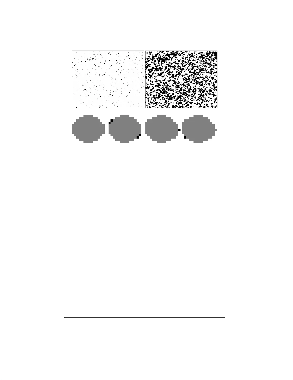
1 Statistical asp ects of birth–and–gro wth sto c hastic pro cesses Giacomo Aletti, Enea G. Bongiorno, Vincenzo Capasso Department o f Mathematics, Universit y of Milan, via Saldini 50, 10133 Milan Italy giacomo.al etti@mat.u nimi.it bongio@mat .unimi.it vincenzo.c apasso@mat .unimi.it Summary . The pap er considers a particular family of set–v alued sto c hastic pro- cesses mo deling birth–and–grow th pro ces ses. The prop osed setting allow s us to in- vestig ate the nucleation and t he gro wth pro cesses . A d eco mp osi tion theorem is es- tablished to c haracterize the nucleatio n and the gro wth . As a consequence, differen t consisten t set–v alued estimators are studied for growth pro cess. Moreov er, th e nu- cleation process is studied via the hitting function, and a consistent estimator of the nucleati on hitting function is derived. In tr oduction Nucleation and gro wth pro cess es arise in several natural and technolog ical applica- tions (cf. [5, 6] and th e references therein) su c h as, for example, solidification and phase–transition of materials, semiconductor crystal grow th, biomineralization, and DNA replication (cf., e.g., [17]). During the years, several authors studied sto c hastic spatial pro cesses (cf. [10, 23, 31] and references therein) nevertheless they essen tially consider static app ro ac hes mo deling real phenomenon s. F or what concerns the dy- namical p oin t of view, a parametric birth–and–gr owth pr o c ess was studied in [25, 26]. A birth–and–gro wth pro cess is a RaCS family given by Θ t = S n : T n ≤ t Θ t T n ( X n ), for t ∈ R + , where Θ t T n ( X n ) is the RaCS obtained as the evol u tion up to time t > T n of the germ b orn at (random) t ime T n in ( ra ndom) location X n , according t o some gro wth model. A n analytical approac h is often used to mo del birth–and–gro wth pro- cess, in particular it is assumed that the gro wth of a sph eric al nucleus of infinitesimal radius is driven according to a non–negativ e normal velocit y , i.e. for ev ery instan t t , a b order point of the crystal x ∈ ∂ Θ t “gro ws” along the out w ards normal unit (e.g. [3, 4, 8, 16]). In view of the c h o sen framew ork, different parametric and n o n– parametric estimations are prop osed o ver the y ears (cf. [2, 5, 7, 9, 12, 24, 27] and references therein). Note that the existence of the outw ards normal vector imp oses a regulari ty condition on ∂ Θ t (and also on the nucleatio n process: it cannot be a p oi nt pro cess). On th e other hand, it is wel l k no wn th at random sets are particular cases of fuzzy 2 Statistic al asp e cts of set–val ue d c ontinuous t i me st o chastic pr o c esses sets. No w, in the class of all convex fuzzy sets ha ving compact supp o rt, Doob –typ e decomp os ition for sub- and sup er–martingales w as studied (e.g. [13–15, 32]). Nev- ertheless, a more general case (than the conv ex one) has not yet b een considered; surely , in order to do this, the first easiest step is to consider decomp ositio n for random set–v alued p rocesses. After which, the step forw ard, to b e considered in a follo wing pap er, can b e to generalize results of this pap er to birth –and – gro wth fuzzy set–v alue pro cesses. This paper is an attempt t o offer an original approac h based on a p u rely geometric stochastic p oin t of view in order to a voi d regularit y assumptions describing birth– and–gro wth pro cess es. The pioneer w ork [21] studies a growth mod el for a single conv ex crystal based on Minko wski sum, whilst in [1], the authors derive a compu- tationally tractable math ematical mo del of such p rocesses that emp hasi zes th e geo- metric growth of ob jects without regularit y assumptions on the boun dary of cry sta ls. Here, in v ie w of this approac h , we introd uce different set–v alued p ara metric estima- tors of the rate of growth of the pro cess . They arise naturally from a decomp ositio n via Minko wski sum and they are consistent as th e observ ation window exp an d s t o the whole space. On the other h an d , keeping in mind that distribut ions of random closed sets are determined by Choqu et capacity functionals and that the nucleation process cannot be observed directly , the pap er p ro vides an estimation pro cedures of the hitting function of the nuclea tion pro ces s. The article is organized as follow s. Section 1.1 contains p reliminary properties. Sec- tion 1.2 introduces a birth–and–gro wth model for random closed sets as the com bi- nation of t wo set–v alued pro cesses (nucleation and gro wth resp ectiv ely) . F urth er, a decomp os ition theorem is established to chara cterize the nuclea tion and the gro wth. Section 1.3 stu dies different estimators of the gro wth p rocess and correspondent con- sisten t prop erties are prove d. I n Section 1.4, t h e nucleation pro cess is studied via the hitting function, and a consistent estimator of the nucleation hitting function is derived. 1.1 Pr eli minary results Let N , Z , R , R + b e the sets of all non–negative integer, integ er, real and non–negative real n u m b ers resp ectiv ely , and let X = R d . Let F be the family of all closed subsets of X and F ′ = F \ {∅} . The suffixes b , k and c denote bound edness, compactness and conv exity properties resp ectiv ely (e.g. F kc denotes t he family of all compact con vex subsets of X ). F or all A, B ⊆ X and α ∈ R + , let us define A + B = { a + b : a ∈ A, b ∈ B } = S b ∈ B b + A, (Minko wski Sum) , α · A = αA = { αa : a ∈ A } , (Scalar Prod uct) , A ⊖ B = ` A C + B ´ C = T b ∈ B b + A, (Minko wski Subtraction) , ˇ A = {− a : a ∈ A } , (Symmetric Set) , where A C = { x ∈ X : x 6∈ A } is the complementary set of A , x + A means { x } + A (i.e. A translate by vector x ) , and, by defi nitio n, ∅ + A = ∅ = α ∅ . I t is well kn o wn that + is a comm u tativ e and associative op eration with a neutral element but, in general, A ⊆ X does not admit opposite ( cf . [18, 29]) and ⊖ is n ot the inve rse op eration of +. The follo wing relations are useful in the sequel (see [30]): for every A, B , C ⊆ X Nov ember 3, 2018 Giacomo Aletti, Enea G. Bongiorno, Vincenzo Capasso 3 ( A ∪ B ) + C = ( A + C ) ∪ ( B + C ) , if B ⊆ C, A + B ⊆ A + C , ( A ⊖ B ) + ˇ B ⊆ A and ( A + B ) ⊖ ˇ B ⊇ A, ( A ∪ B ) ⊖ C ⊇ ( A ⊖ C ) ∪ ( B ⊖ C ) . In the follo wing, w e shall work with closed sets. In general, if A, B ∈ F then A + B does not belong to F (e.g. , in X = R let A = { n + 1 /n : n > 1 } and B = Z , then { 1 /n = ( n + 1 /n ) + ( − n ) } ⊂ A + B and 1 /n ↓ 0, but 0 6∈ A + B ) . I n view of this fact, we define A ⊕ B = A + B where ( · ) den o tes th e closure in X . It can b e prov ed that, if A ∈ F and B ∈ F k then A + B ∈ F (see [30]). F or any A, B ∈ F ′ the Hausdorff distanc e (or metric ) is defin ed by δ H ( A, B ) = max  sup a ∈ A inf b ∈ B k a − b k X , sup b ∈ B inf a ∈ A k a − b k X ff . A random closed set (RaCS) is a map X d efined on a probabilit y space ( Ω , F , P ) with v alues in F such th at { ω ∈ Ω : X ( ω ) ∩ K 6 = ∅} is measurable for eac h compact set K in X . It can b e pro ved (see [19]) that, if X, X 1 , X 2 are RaCS and if ξ is a measurable real–v alued function, then X 1 ⊕ X 2 , X 1 ⊖ X 2 , ξ X and (Int X ) C are RaCS. Moreo ver, if { X n } n ∈ N is a sequence of RaCS then X = S n ∈ N X n is so. Let X b e a RaCS, then T X ( K ) = P ( X ∩ K 6 = ∅ ), for all K ∈ F k , is its hitting function (or Cho quet c ap acity functional ). The well k no wn Matheron Theorem states that, the probability law P X of any RaCS X is uniquely determined by its hitting function (see [20]) and hence by Q X ( K ) = 1 − T X ( K ). Remark 1.1 ( Se e [ 22].) If b oth X and Y a re R aC S , then, for every K ∈ F k , T X ⊕ Y ( K ) = E ˆ E ˆ T X ` K ⊕ ˇ Y ´ ˛ ˛ Y ˜˜ . Moreo ver, if X, Y are indep endent, then, for every K ∈ F k , T X ∪ Y ( K ) = T X ( K ) + T Y ( K ) − T X ( K ) T Y ( K ) . A RaCS X is stationary if the probability law s of X and X + v coincide for every v ∈ X . Thus, t h e hitting function of a stationary RaCS clearly is in vari ant up to translation T X ( K ) = T X ( K + v ) for each K ∈ F k and an y v ∈ X . A stationary RaCS X is er go dic , if, for all K 1 , K 2 ∈ F , 1 | W n | Z W n Q X (( K 1 + v ) ∪ K 2 ) dv → Q X ( K 1 ) Q X ( K 2 ) , as n → ∞ ; where { W n } n ∈ N is a c onvex aver aging se quenc e of sets in X (see [11]), i.e. eac h { W n } is con vex and compact, W n ⊂ W n +1 for all n ∈ N and sup { r ≥ 0 : B ( x, r ) ⊂ W n for some x ∈ W n } ↑ ∞ , as n → ∞ . Proposition 1.2 Let X , Y be R a CS with Y ∈ F ′ k a.s. and X stationary , t hen X + Y is a stationary R aC S . Moreo ver, if X is ergod i c, then X + Y is so. Nov ember 3, 2018 4 Statistic al asp e cts of set–val ue d c ontinuous t i me st o chastic pr o c esses Proof. Let Z = X + Y , it is a RaCS. Note that T Z ( K ) = E ˆ E ˆ T X ` K + ˇ Y ´ ˛ ˛ Y ˜˜ = E ˆ E ˆ T X ` K + ˇ Y + v ´ ˛ ˛ Y ˜˜ = T Z ( K + v ) , for every K ∈ F k and v ∈ X , then Z = X + Y is stationary . F urther, let us supp ose that X is ergodic, then, by T onelli’s Theorem and by dominated conv ergence theorem, w e obtain Z W n Q Z (( K 1 + v ) ∪ K 2 ) | W n | dv = E » E » 1 | W n | Z W n Q X ((( K 1 + v ) ∪ K 2 ) + ˇ Y ) dv ˛ ˛ ˛ ˛ Y –– → E ˆ E ˆ Q X ( K 1 + ˇ Y ) Q X ( K 2 + ˇ Y ) ˛ ˛ Y ˜˜ = Q Z ( K 1 ) Q Z ( K 2 ) , for every K 1 , K 2 ∈ F k . Hence X + Y is ergo dic.  1.2 A Birt h–a nd–Gro wth pro cess Let ( Ω , F , { F n } n ∈ N , P ) b e a filtered probability sp ace with th e usual prop erties. Let { B n : n ≥ 0 } and { G n : n ≥ 1 } b e tw o families of R aC S such that B n is F n – measurable and G n is F n − 1 –measurable. These pro ces ses rep resent th e birth ( o r nucle ation ) pr o c ess and the gr owth pr o c ess respectively . Th us, let us define recur- sive ly a birth–and–gro wth pro ces s Θ = { Θ n : n ≥ 0 } by Θ n =  ( Θ n − 1 ⊕ G n ) ∪ B n , n ≥ 1 , B 0 , n = 0 . (1.1) Roughly sp eaking, Equ atio n (1.1) means that Θ n is the enlarge ment of Θ n − 1 due to a Minko wski gr owth G n while nucle ation B n occurs. Without loss of general ity let us consider the foll o wing assumption. (A-1) F or every n ≥ 1, 0 ∈ G n . Note that, Assumption (A-1) is equiv alent to Θ n − 1 ⊆ Θ n . In [1], the authors d erive (1.1) from a contin uous time birth–and–gro wth pro cess ; here, in order to make in ference, the discrete t ime case is su fficient. Indeed, a sample of a b ir th–and–gro wth pro ces s is usually a time sequence of pictures that represent process Θ at d ifferent temp oral step; namely Θ n − 1 , Θ n . Thus, in view of (1.1), it is interes ting to inv estigate { G n } and { B n } ; in particular, we sh a ll estimate the maximal grow th G n and the capacity functional of B n . F or the sak e of simplicity , Y , X , G and B will d enote RaCS Θ n , Θ n − 1 , G n and B n respectively (then X ⊆ Y ). Thus, let us consider the follo wing general definition. Definition 1.3 Let Y , X be RaCS with X ⊆ Y . A X –de c omp osition of Y is a couple of RaCS ( G, B ) for whic h Y = ( X ⊕ G ) ∪ B . (1.2) Note that, since we can consider ( G, B ) = ( { 0 } , Y ), there alw ays exists a X – decomp os ition of Y . It can happ en that G and B in (1.2) are not uniqu e. As ex ample, let Y = [0 , 1] and X = { 0 } , then b oth ( G 1 , B 1 ) = ( Y , Y ) and ( G 2 , B 2 ) = ( X, Y ) Nov ember 3, 2018 Giacomo Aletti, Enea G. Bongiorno, Vincenzo Capasso 5 satisfy (1.2). As a consequence, since we can not d istinguish b et w een tw o different decomp os itions, w e shall choose a maximal one according t o the follo wing prop osi- tion. Proposition 1.4 (Se e [30]) Let Y , X b e RaCS with X ⊆ Y . Then G = Y ⊖ ˇ X = { g ∈ X : g + X ⊆ Y } . (1.3) is the greatest R aC S, with respect to set inclusion, such that ( X ⊕ G ) ⊆ Y . Corollary 1.5 The couple ( G = Y ⊖ ˇ X , B = Y ∩ ( X ⊕ G ) C ) is th e m ax -min X – decomp os ition of Y . As a consequ en ce, ( G, B ) is a X –decomp ositio n of Y and for any other X –decomposition of Y , say ( G ′ , B ′ ), then G ′ ⊆ G and B ′ ⊇ B . In other words, if X , G ′ , B ′ are RaCS and Y = ( X ⊕ G ′ ) ∪ B ′ , th en G = Y ⊖ ˇ X ⊇ G ′ and Y = ( X ⊕ G ) ∪ B ′ . Let Θ be as in (1.1). F rom now on, G n denotes Θ n ⊖ ˇ Θ n − 1 that, as a conseq u ence of Assumption (A-1), con tains the origin. Moreo ver, w e shall supp os e (A-2) There exists K ∈ F ′ b such that G n = Θ n ⊖ ˇ Θ n − 1 ⊆ K for eve ry n ∈ N . (A-3) F or every n ≥ 1, ` B n ⊖ ˇ Θ n − 1 ´ = ∅ almost surely . Roughly sp eaking, Assumption (A -2) means t h at pro cess Θ does not grow too “fast” , whilst Assumption (A-3) m eans th at it cannot b orn something that, up to a trans- lation, is larger (or equal) than what there already exists. Let us remark that A ssumption (A-2) implies { G n } ⊂ F ′ k and X ⊕ G n = X + G n , for any RaCS X . 1.3 Est im ators of G On th e one h an d Prop o sition 1.4 giv es a theoretical formula for G , but, on the other hand, in practical cases , data are b ounded by some observ ation window and edge effects may cause problems. Hence, as the standard statistical scheme for spatial processes (e.g. [23]) suggests, we w onder if there exists a consisten t estimator of G as the observ ation window expands to the whole space X . Proposition 1.6 If { W i } i ∈ N ⊂ F ′ ck is a con vex a veraging sequence of sets, then , for any K ∈ F ′ k , X = S i ∈ N W i ⊖ ˇ K . In this case, we say that { W i } i ∈ N expands t o X and w e shall write W i ↑ X . Proof. At first note that X = S i ∈ N Int W i and for an y i ∈ N , W i ⊆ W i +1 . Let x ∈ X and K ∈ F ′ k . Note t hat, x + K ∈ F ′ k is a compact set. Then there exists a finite family of ind i ces I ⊂ N suc h th at, if N = max I , then x + K ⊆ [ j ∈ I Int W j = Int W N . Hence, w e hav e that x ∈ Int W N ⊖ ˇ K ⊆ W N ⊖ ˇ K , i.e., for any x ∈ X , there exists n 0 ∈ N such that x ∈ W n 0 ⊖ ˇ K .  Nov ember 3, 2018 6 Statistic al asp e cts of set–val ue d c ontinuous t i me st o chastic pr o c esses Let W ∈ { W i } i ∈ N b e an observ ation window and let us denote b y Y W and X W , th e (random) observ ation of Y an d X through W , i.e. Y ∩ W and X ∩ W respectively . Let u s consider the estimator of G given by th e maximal X W –decomposition of Y W : b G W = ` Y W ⊖ ˇ X W ´ (1.4) so that X W ⊕ b G W ⊆ Y W ⊆ W . Notice th a t, whenever Y and X are b ounded, then there exists W j ∈ { W i } i ∈ N such that Y ⊆ W j and ˇ X ⊆ W j , hence b G W j = Y ⊖ ˇ X = G . In other words, on th e set { ω ∈ Ω : X ( ω ) , Y ( ω ) boun ded } , th e estimator (1.4) is consisten t b G W i ( Y , X | Y , X b ounded) → G, as W i ↑ X ; otherwise, as we already said, if Y and X are unbounded, edge effects ma y cause problems and the estimator (1.4) is, in general, not consisten t as w e discussed in the follo wing example. Example 1.7 Let X = R 2 , let us consider X = ( { x = 0 } ∪ { y = 0 } ) and Y = X + B (0 , 1) where B (0 , 1) is the closed unit ball centered in the origin. S urely X ⊂ Y , and they are unbound ed. N ote that Y = ( X + G ) for any G such that ( { 0 } × [ − 1 , 1] ∪ [ − 1 , 1] × { 0 } ) ⊆ G ⊆ B (0 , 1). On the other hand , by Prop osi tion 1.4, there ex i sts a un iq ue G that is the greatest set, with resp ect to set inclusion; in this case G = [ − 1 , 1] × [ − 1 , 1]. Let us su p pose 0 ∈ W 0 and let W ∈ { W i } i ∈ N , then, by Eq u atio n (1.4), the estimator of G is b G W = { 0 } 6 = G . This is an edge effect due to th e fact t hat, for every G ′ with { 0 } ⊂ G ′ ⊆ G , it holds ( X W + G ′ ) ∩ W C 6 = ∅ and then X W + G ′ 6⊆ Y W that do es not agree with Proposition 1.4. Edge effects can b e reduced by considering the foll o wing estimators of G b G 1 W = ` Y W ⊖ ˇ X W ⊖ ˇ K ´ ∩ K , (1.5) b G 2 W = “h Y W ∪ “ ∂ + K W X W ”i ⊖ ˇ X W ” ∩ K ; (1.6) where K is given in A ss umption (A-2) and where ` ∂ + K W X W ´ = ( X W + K ) \ W . The role of K will be clarified in Prop ositio n 1.8 where it guarantees the monotonicit y of b G 1 W . Note th at, estimators (1.5) (1.6) are b ounded (i.e. compact) RaCS, moreo ver, if Y and X are b ounded, then b G 1 W j , b G 2 W j even tually coincide with the estimator (1.4); i.e. there exists n 0 such that for all j ≥ n 0 , b G W j = b G 1 W j = b G 2 W j = G . Let us explain ho w b G 1 W and b G 2 W w ork . Estimator b G 1 W is obtained by reducing th e information given by X to th e smaller window W ⊖ ˇ K , whilst Y is observed in W . Then b G 1 W is the grea test sub se t of K , with respect to set inclusion, suc h that X W ⊖ ˇ K + b G 1 W ⊆ Y W (see Prop os ition 1.4). Estimator b G 2 W is obtained by observing X in W (and not W ⊖ ˇ K ), whilst Y is increased (at least) by ` ∂ + K W X W ´ , that is the greatest p ossible set of gro wth for X outside of th e observed window W . Then b G 2 W is th e greatest subset of K , with respect to set inclusion, such that ( X W + b G 2 W ) ∩ W ⊆ Y W , or, alternativel y , X W + b G 2 W ⊆ Y W ′ , where Y W ′ = Y W ∪ ` ∂ + K W X W ´ (see Proposition 1.4 ). Note that by definition of Minko wski Subtraction Nov ember 3, 2018 Giacomo Aletti, Enea G. Bongiorno, Vincenzo Capasso 7 b G 1 W = T x ∈ X W ⊖ ˇ K x + (( − x + K ) ∩ Y W ) , b G 2 W = T x ∈ X W x + (( − x + K ) ∩ Y W ′ ) ; i.e. every x ∈ X W ⊖ ˇ K (resp. x ∈ X W ) “gro ws” at most as ( − x + K ) ∩ Y W (resp. ( − x + K ) ∩ Y W ′ ). Now , we are ready to show the consistency p roperty of b G 1 W i and b G 2 W . In particular, Proposition 1.8 prov es that b G 1 W i decreases, with resp ect to set inclusion, to the theoretical G , whenever W i expands to the whole sp a ce ( W i ↑ X ). Prop osition 1.9 prov es that, for every W ∈ F ′ , b G 2 W is a better estimator than b G 1 W and hence it is a consisten t estimator of G . Proposition 1.8 Let Y , X b e RaCS, let 0 ∈ G = Y ⊖ ˇ X ⊆ K . The follow ing statements hold for b G 1 W : (1) G ⊆ b G 1 W for every W ; (2) b G 1 W 2 ⊆ b G 1 W 1 if W 2 ⊇ W 1 ; (3) If W i ↑ X , then T i ∈ N b G 1 W i = G . Moreo ver, lim i →∞ δ H ( b G 1 W i , G ) = 0 . (1.7) Proof. (1) Since 0 ∈ K , T k ∈ K − k + W = W ⊖ ˇ K ⊆ W and then X W ⊖ ˇ K ⊆ W . Let g ∈ G , t hen g + X ⊆ Y . Since g ∈ K , last inclusion still holds when X and Y are substituted b y X W ⊖ ˇ K and Y W respectively: g + X W ⊖ ˇ K ⊆ Y W . Thus g ∈ b G 1 W follo ws by Definition (1.5) and Prop os ition 1.4. (2) In order to obtain b G 1 W 2 ⊆ b G 1 W 1 , it is su ffici ent to prove that X W 1 ⊖ ˇ K + b G 1 W 2 ⊆ Y W 1 (1.8) since b G 1 W 1 is th e greatest set, with resp ect to set in clu sion, for which the inclusion (1.8) holds. In fact, W 1 ⊖ ˇ K ⊆ ` W 1 ⊖ ˇ K ´ + K ⊆ W 1 ⊆ W 2 , th en X W 1 ⊖ ˇ K ⊆ X W 2 . Let x ∈ X W 1 ⊖ ˇ K = X ∩ ` W 1 ⊖ ˇ K ´ , then x ∈ X W 2 . By definition of b G 1 W 2 , w e have x + b G 1 W 2 ⊆ Y W 2 ⊆ Y . On the other hand, since x ∈ W 1 ⊖ ˇ K and b G 1 W 2 ⊆ K , we ha ve x + b G 1 W 2 ⊆ ` W 1 ⊖ ˇ K ´ + K ⊆ W 1 ; i.e. x + b G 1 W 2 is included both in Y and in W 1 . (3) Since G ⊆ T i ∈ N b G 1 W i , it remains t o prov e that \ i ∈ N b G 1 W i ⊆ G ; i.e. if g ∈ b G 1 W i for eac h i ∈ N , then g ∈ G . T ak e g ∈ T i ∈ N b G 1 W i . By definition of b G 1 W 1 , w e have g + x ∈ Y for all x ∈ X W i ⊖ ˇ K and ∀ i ∈ N . (1.9) Nov ember 3, 2018 8 Statistic al asp e cts of set–val ue d c ontinuous t i me st o chastic pr o c esses By contradiction, assume g 6∈ G . Then g + X 6⊆ Y , i.e. there exists x ∈ X such that ( g + x ) 6∈ Y . On the one hand , Proposition 1.6 implies that there ex ists j ∈ N such that x ∈ W j ⊖ ˇ K . On the other hand, Equation (1.9) implies g + x ∈ Y which is a contra diction. Thus Theorem 1.1.18 in [19] implies (1.7).  Proposition 1.9 F or every W ∈ F ′ , G ⊆ b G 2 W ⊆ b G 1 W . Proof. Let us d ivide th e pro of in tw o parts; in t h e first one w e prove that b G 2 W ⊆ b G 1 W , in the second one that G ⊆ b G 2 W . Let g ∈ b G 2 W and x ∈ X W ⊖ ˇ K . S i nce b G 2 W ⊆ K , we hav e x + g ∈ ` W ⊖ ˇ K ´ + b G 2 W ⊆ ` W ⊖ ˇ K ´ + K ⊆ W ; (1.10) where w e u se prop erties of monotonicit y of th e Minkwoski S ubtraction and Sum. Moreo ver, by definition of b G 2 W , x + g ∈ Y W , or x + g ∈ “ ∂ + K W X W ” ⊆ W C . By ( 1 .10), x + g ∈ Y W . The arbitrary choice of x ∈ X W ⊖ ˇ K completes the first p a rt of the pro of. F or the second part, let g ∈ G and x ∈ X W . By definition of G , x + g ∈ Y . W e ha ve tw o cases: - x + g ∈ W , and therefore x + g ∈ Y W , - x + g 6∈ W . Since x ∈ X W , x + g ∈ ( X W + G ) \ W ⊆ ` ∂ + K W X W ´ .  Corollary 1.10 b G 2 W is consisten t (i.e. b G 2 W ↓ G whenever W ↑ X ). A Gener al Definition of b G 2 W . The follo wing p roposition shows that the esti- mator in (1.6) can be defi ned in an equiv alent w a y by b G 2 W ( Z ) = nh Y W ∪ “ ∂ + K W Z ”i ⊖ ˇ X W o K ; where ` ∂ + K W X ´ in ( 1 .6) is substituted by ` ∂ + K W Z ´ with X W \ ( W ⊖ ˇ K ) ⊆ Z ⊆ W. (1.11) In other w ords, we are sa y in g that, under condition (1.11), b G 2 W ( Z ) do es not d ep end on Z . F rom a computational point of view, this means that Z can b e c hosen in a w ay th at reduces th e computational costs. On the one hand, the best c hoice of Z seems to b e the smallest p ossible set, i.e. Z = X W \ ( W ⊖ ˇ K ) . On the other hand, in order to get X W \ ( W ⊖ ˇ K ) , we h a ve to compute ` W ⊖ ˇ K ´ that may be costly if at least on e b etw een W and K has a “bad shap e” (for instance it is not a rectangular one). Proposition 1.11 If Z 1 , Z 2 ∈ P ′ b oth satisfy condition (1.11), then b G 2 W ( Z 1 ) = b G 2 W ( Z 2 ). Nov ember 3, 2018 Giacomo Aletti, Enea G. Bongiorno, Vincenzo Capasso 9 Fig. 1. 1. W e consider t wo pictures of a simulated birth–and–growth p rocess, at tw o different time instan ts, that in our notations are X and Y . Emp hasi zing the differences, w e rep ort here the magnified pictures of t h e true gro wth used for the sim u la t io n , the compu t ed b G 2 W , b G 1 W and b G 1 W ⊖ ˇ K . Note t hat they agree with Prop o- sition 1.8 and Proposition 1.9 since b G 1 W ⊖ ˇ K ⊇ b G 1 W ⊇ b G 2 W . Proof. It is sufficien t to prov e: (1) Z 1 ⊆ Z 2 implies b G 2 W ( Z 1 ) ⊆ b G 2 W ( Z 2 ); (2) b G 2 W ( W ) ⊆ b G 2 W “ X W \ ( W ⊖ ˇ K ) ” . In fact, (1) and (2) imp ly that b G 2 W ( W ) = b G 2 W “ X W \ ( W ⊖ ˇ K ) ” . At the same time they imply b G 2 W ( Z ) = b G 2 W “ X W \ ( W ⊖ ˇ K ) ” holds for every Z that satisfies (1.11 ); that is the thesis. STEP (1) is a consequence of the follo wing implications Z 1 ⊆ Z 2 ⇒ Z 1 + K ⊆ Z 2 + K, ⇒ Y W ∪ [ ( Z 1 + K ) \ W ] ⊆ Y W ∪ [ ( Z 2 + K ) \ W ] , ⇒ b G 2 W ( Z 1 ) ⊆ b G 2 W ( Z 2 ); where the last one holds since X 1 ⊖ Y ⊆ X 2 ⊖ Y if X 1 ⊆ X 2 (see [30]). Before proving the second step, we show that b G 2 W ( Z ) = b G 2 W “ Z W \ ( W ⊖ ˇ K ) ” for all Z t h at satisfies (1.11). This statement is true if “ Z W \ ( W ⊖ ˇ K ) + K ” \ W and ( Z + K ) \ W are th e same set. Since Minko wski sum is distribu t i ve with resp ect to union, we get Nov ember 3, 2018 10 S tatistic al asp e cts of set–val ue d c ontinuous t i me st o chastic pr o c esses ( Z + K ) \ W = h“ Z W \ ( W ⊖ ˇ K ) ∪ Z W ⊖ ˇ K ” + K i \ W = h“ Z W \ ( W ⊖ ˇ K ) + K ” \ W i ∪ ˆ` Z W ⊖ ˇ K + K ´ \ W ˜ . Then w e hav e to pro ve that ˆ` Z W ⊖ ˇ K + K ´ \ W ˜ = ∅ : ` Z W ⊖ ˇ K + K ´ \ W = ˘ˆ Z ∩ ` W ⊖ ˇ K ´˜ + K ¯ \ W ⊆ ˘ ( Z + K ) ∩ ˆ` W ⊖ ˇ K ´ + K ˜¯ \ W ⊆ [( Z + K ) ∩ W ] \ W = ∅ . STEP (2) . Since b G 2 W ( X W ) = b G 2 W “ X W \ ( W ⊖ ˇ K ) ” , thesis b ecomes b G 2 W ( W ) ⊆ b G 2 W ( X W ). Let g ∈ b G 2 W ( W ) . W e m u st prov e g ∈ b G 2 W ( X W ), i.e. for every x ∈ X W g + x ∈ Y W , or g + x ∈ ( X W + K ) \ W. Since g ∈ b G 2 W ( W ) , for any x ∈ X W w e can h a ve tw o p ossi bilities (a) g + x ∈ Y W , (b) g + x ∈ ( W + K ) \ W . It remains to prove th at (b) implies g + x ∈ ( X W + K ) \ W . I n particular, (b ) implies g + x ∈ W C . At the same time g + x ∈ X W + K , i.e. g + x ∈ ( X W + K ) \ W .  1.4 Hit ting F u nction Asso ciated to B In many practical cases, an observer, through a window W and at tw o different instants, observes the nucleation and gro wth processes namely X and Y . According to Section 1.3 w e can estimate G v i a the consistent estimator b G 2 W or b G 1 W (in t h e follo wing we shall write b G W meaning one of them). F rom the birth–and–gro wth process p oint of view, it is also interesting to test whenever the nuclea tion process B = { B n } n ∈ N is a sp eci fic RaCS (for example a Bo ol ean model or a point p ro - cess). In general, we cannot directly observ e the n –th nucleation B n since it can b e o verlapped by other nuclei or by their evolutions. Nevertheless, we shall infer on the hitting function associated to the nucleation process T B n ( · ). Let us consider the decomp os ition given by (1.2) Y = ( X + G ) ∪ B then the follow ing prop osition is a consequence of Remark 1.1. Proposition 1.12 If ( G, B ) is a X –decomposition of Y suc h that B is indep enden t on X and on G , then, for each K ∈ F k , T Y ( K ) = T X + G ( K ) + T B ( K ) − T X + G ( K ) T B ( K ) , that, in terms of Q · ( K ) = (1 − T · ( K )), is equiv alen t t o Q Y ( K ) = Q B ( K ) Q X + G ( K ) . In other words, the probabilit y for the exploring set K to miss Y is the probability for K to miss B m ultiplied by the probabilit y for K to miss X + G . Nov ember 3, 2018 Giacomo Aletti, Enea G. Bongiorno, Vincenzo Capasso 11 Remark 1.13 W orking with d ata we shall consider tw o estimators of the h itting function (w e refer to [23, p. 57–63] and references th erei n). In particular, if X is a stationary ergo dic RaCS, then T X ( · ) can b e estimated by a single realization of X and t w o empirical estimators are giv en by b T X,W ( K ) = µ λ `` X + ˇ K ´ ∩ ( W ⊖ K 0 ) ´ µ λ ( W ⊖ K 0 ) , K ∈ F k ; where µ λ is the Lebesgue measure on X = R d and K 0 is a compact set suc h that K ⊂ K 0 for all K ∈ F k of in terest. A r e gular close d set in X is a closed set G ∈ F ′ for whic h G = Int G ; i.e. G is the closure (in X ) of its interio r. Proposition 1.14 Le t G ∈ F ′ k b e a regular closed subset in X . Then, for every X ∈ F ′ , X + G is a regular closed set. Proof. S ince X + G is a closed set, Int ( X + G ) ⊆ X + G . It remains to prov e t hat X + G ⊆ Int ( X + G ). Let y ∈ X + G , then there ex is ts x ∈ X and g ∈ G suc h that y = x + g . If g ∈ I n t G , then t h ere exists an op en neighborho od of g for whic h U ( g ) ⊆ Int G and x + U ( g ) is an open n eighborh o od of x + g included in X + G ; i.e. x + g ∈ Int ( X + G ). On the other hand, let g ∈ ∂ G = G \ Int G , then there exists { g n } n ∈ N ⊂ G su c h th at g n → g and g n ∈ Int G , for all n ∈ N . Th u s, for every n ∈ N , x + g n is an in terior point of X + G and x + g n → x + g ∈ Int ( X + G ).  Proposition 1.15 (Se e [23, The or em 4.5 p. 61] and r efer enc es ther ein) Let X b e an ergodic stationary random closed set. I f the random set X is almost surely regular closed sup K ∈ F k K ⊆ K 0 ˛ ˛ ˛ b T X,W ( K ) − T X ( K ) ˛ ˛ ˛ → 0 , a.s. (1.12) as W ↑ X an d for every K 0 ∈ F ′ . Remark 1.16 Proposition 1.14, together to Equation ( 1 .1) means that, if { G n } n ∈ N is a sequence of almost su rel y regular closed sets, t hen { Θ n } n ∈ N is so. The follow ing Theorem sh o ws that the hitting functional Q B of the hidden nucleatio n process can b e exstimated by the observ able quantit y e Q B,W , where for every K ∈ F k , e Q B,W ( K ) := b Q Y ,W ( K ) b Q X + b G W ,W ( K ) , (1.13) and b G W is giv en by (1.5) or (1.6). Nov ember 3, 2018 12 S tatistic al asp e cts of set–val ue d c ontinuous t i me st o chastic pr o c esses Theorem 1. 17 Let X , Y be tw o RaCS a.s. regular closed. Let ( G, B ) b e a X – decomp os ition of Y with B a stationary ergo dic RaCS indep endent on G and X . Assume that G is an a.s. regular closed set and e Q B,W defined in Equ atio n (1.13). Then, for any K ∈ F k , ˛ ˛ ˛ e Q B,W ( K ) − Q B ( K ) ˛ ˛ ˛ − → W ↑ X 0 , a.s. Proof. Let K ∈ F k b e fi xed. F or the sake of simplicit y , Q · , e Q · and b Q · denote Q · ( K ), e Q · ,W ( K ) and b Q · ,W ( K ) resp ectiv ely . Thus, ˛ ˛ ˛ e Q B − Q B ˛ ˛ ˛ = ˛ ˛ ˛ ˛ ˛ ˛ b Q Y b Q X + b G W − Q Y Q X + G ˛ ˛ ˛ ˛ ˛ ˛ = ˛ ˛ ˛ ˛ ˛ ˛ b Q Y Q X + G − Q Y b Q X + b G W b Q X + b G W Q X + G ˛ ˛ ˛ ˛ ˛ ˛ . Since Y ⊇ X + b G W , b Q X + b G W > b Q Y . Accordingly to (1.12), b Q Y conv erges to Q Y that is a p ositive quantit y . Th us, thesis is eq uiv alent to prov e th at ˛ ˛ ˛ b Q Y Q X + G − Q Y b Q X + b G W ˛ ˛ ˛ → 0 , a.s. as W ↑ X . The follo wing inequalities hold ˛ ˛ ˛ b Q Y Q X + G − Q Y b Q X + b G W ˛ ˛ ˛ ≤ Q X + G ˛ ˛ ˛ b Q Y − Q Y ˛ ˛ ˛ + Q Y ˛ ˛ ˛ Q X + G − b Q X + b G W ˛ ˛ ˛ ≤ Q X + G ˛ ˛ ˛ b Q Y − Q Y ˛ ˛ ˛ + Q Y ˛ ˛ ˛ Q X + G − Q X + b G W ˛ ˛ ˛ + Q Y ˛ ˛ ˛ Q X + b G W − b Q X + b G W ˛ ˛ ˛ . Proposition 1.2 and Proposition 1.14 gu arantee that X + G is a stationary ergo d ic RaCS and a.s. regular closed, then w e can apply (1.12) to the first an d the third addends. It remains to pro ve that ˛ ˛ ˛ Q X + G − Q X + b G W ˛ ˛ ˛ → 0 as W ↑ X . (1.14) Since Mink o wski sum is a contin uou s map from F × F k to F (see [30]), b G W ↓ G a.s. implies X + b G W ↓ X + G a.s. A s a consequence, we get that X + b G W ↓ X + G in distribution [28, p. 182], whic h is Equation (1.14 ).  References 1. G. Aletti, E. G. Bongiorno, and V. Capasso, A set–v alued framew ork for birth– and–gro wth processes. (su b mitted). 2. G. Aletti and D. S a ada, Surviv al analysis in Johnson–Mehl tessellation, Stat. Inference S toch. Pro cess ., 11 (2008) 55–76. 3. M. Burger, V. Capasso, and A. Micheletti, An extension of the Kolmogoro v – Avrami form ula to inhomogeneous birth–and–gro wth pro cesses, in: G. Aletti et al., (Eds.), Math Ev erywhere, Springer, Berlin, 2007 63–76. 4. M. Burger, V. Capasso, and L. Pizzocchero, Mesoscale av eraging of nucleation and gro wth mo dels, Multiscale Model. S i mul., 5 (2006) 564–592. Nov ember 3, 2018 Giacomo Aletti, Enea G. Bongiorno, Vincenzo Capasso 13 5. V . Capasso, (Ed .), Mathematical Mo delling for P olymer Pro cessing. P olymer- ization, Crystallization, Man u f acturing, Mathematics in Indu s try , 2, Springer– V erlag, Berlin, 2003. 6. V . Capasso , On the sto c h astic geometry of gro wth, in: S ekim ura, T. et al., (Eds.), Morphogenesis and Pattern F ormation in Biologica l Sy stems, Sp ringe r, T okyo, 2003 45–58. 7. V . Capasso and E. Villa, Su rviv al functions and contact distribution functions for inhomogeneous, sto c hastic geometric marked p oin t pro cesse s, S toch. Anal. Appl., 23 (2005) 79–96. 8. S . N . Chiu, Johnson–Mehl tessellations: asymptotics and inferences, in: Proba- bilit y , finance and insurance, W orld Sci. Publ., River Edge, NJ, 2004 136–1 49. 9. S . N. Chiu, I. S. Molchano v, and M. P . Quine, Maximum likelihoo d estimation for germination–gro wth processes with app li cation to neurotransmitters data, J. Stat. Comput. Sim ul., 73 (2003) 725–732. 10. N. Cressie, Modeling grow t h with random sets, in: S p atia l statistics and imaging (Brunswic k , ME, 1988), IMS Lecture N otes Monogr. S er. , V ol. 20, In s t. Math. Statist., Ha ywa rd, CA, 1991 31–45. 11. D. J. Daley and D. V ere-Jones, An In trod uction to the Theory of Poin t Pro- cesses. Vol. I, Probability and its Ap p li cations, Springer–V erlag, N ew Y ork, second edition, 2003. 12. T. Erhardsson, Refined d is tributional appro ximations for th e uncov ered set in the Johnson–Mehl model, St oc hastic Process. Appl., 96 (2001) 243–25 9. 13. W. F ei and R. W u, Doob ’s decomp osition th eo rem for fuzzy (sup er) sub ma rtin- gales, Sto chastic Anal. Appl., 22 (2004) 627–645 . 14. Y. F eng, Decomp ositio n theorems for fuzzy sup ermartingales and submartin- gales, F uzzy S ets and Systems, 116 (2000) 225–235. 15. Y. F eng and X. Zhu, S emi-order fuzzy sup ermartingales and submartingales with conti nuous time, F uzzy Sets and Systems, 130 (2002) 75–86. 16. H. J. F rost and C. V. Thompson, The effect of nucleation conditions on the top o logy and geometry of tw o–dimensional grain structures, Act a Metallurgica, 35 (1987) 529–5 40. 17. J. Herrick, S. Jun , J. Bec h hoefer, and A. Bensimon, Kinetic mo del of DNA replication in euk aryotic organisms, J.Mol.Biol ., 320 (2002) 741–750. 18. K. Keimel and W. Roth, Ordered Cones and Ap pro ximation, Lecture Notes in Mathematics, V ol. 1517, Springer–V erlag, Berlin, 1992. 19. S. Li, Y. O gura, and V. Kreinovic h, Limit Theorems and App l ications of Set– V alued and F uzzy Set–V alued Random V ariables, Klu wer Academic Publishers Group, Dordrech t, 2002. 20. G. Matheron, Random Sets and Integ ral Geometry, John Wiley & S ons, New Y ork-Lond on - Sydney , 1975. 21. A. Micheletti, S. Patti, and E. Villa, Crystal grow th simulations: a new math - ematical mo del based on the Minko wski sum of sets, in: D.Aquilano et al., (Eds.), Industry Days 2003-200 4, volume 2 of The MIRIAM Pro ject, Esculapio, Bologna, 2005 130–140 . 22. I. S. Molchano v, Limit Theorems for Unions of Random Closed Sets, Lecture Notes in Mathematics, V ol. 1561, Springer–V erlag, Berlin, 1993. 23. I. S. Molchano v, Statistics of the Boolean Mo del for Practitioners and Mathe- maticians, Wiley , Chic h ester, 1997. Nov ember 3, 2018 14 S tatistic al asp e cts of set–val ue d c ontinuous t i me st o chastic pr o c esses 24. I. S. Molc h ano v and S. N . Chiu, Smo othing techniques and estimation meth- ods for nonstationary Boolean mo dels with applications to co verage processes, Biometrik a, 87 (2000) 265–2 83. 25. J. Møller, R a ndom Johnson–Mehl t es sellations, Adv . in Ap pl. Probab., 24 (1992) 814–844 . 26. J. Møller, Generation of Johnson–Mehl crystals and comparative analysis of mod els for random nucleation, A d v. in Appl. Probab., 27 (1995) 367–383. 27. J. Møller and M. S ørensen, Statistical analysis of a spatial birth – and–death process model with a view to mo delli n g linear dune fields, S cand . J. Statist., 21 (1994) 1–19. 28. H. T. Nguyen, An Introduction to Random Sets, Chapman & Hall/CRC, Boca Raton, FL, 2006. 29. H. R ˚ adstr¨ om, A n emb edding th eo rem for spaces of conv ex sets, Proc. Amer. Math. Soc., 3 (1952) 165–169. 30. J. Serra, Image Analysis and Mathematical Morphology, Academic Press In c. [Harcourt Brace Jov ano vich Pub l ishers], London, 1984. 31. D. Stoy an, W. S. Kendall, and J. Meck e, Stochastic Geometry and its Applica- tions, John Wiley & Sons Lt d ., Chichester, second edition, 1995. 32. P . T er´ an, Cones and decomp osition of sub- and sup ermartingales. F uzzy S ets and Systems, 147 (2004) 465–474. Nov ember 3, 2018