Design and analysis of continuous hybrid differentiator

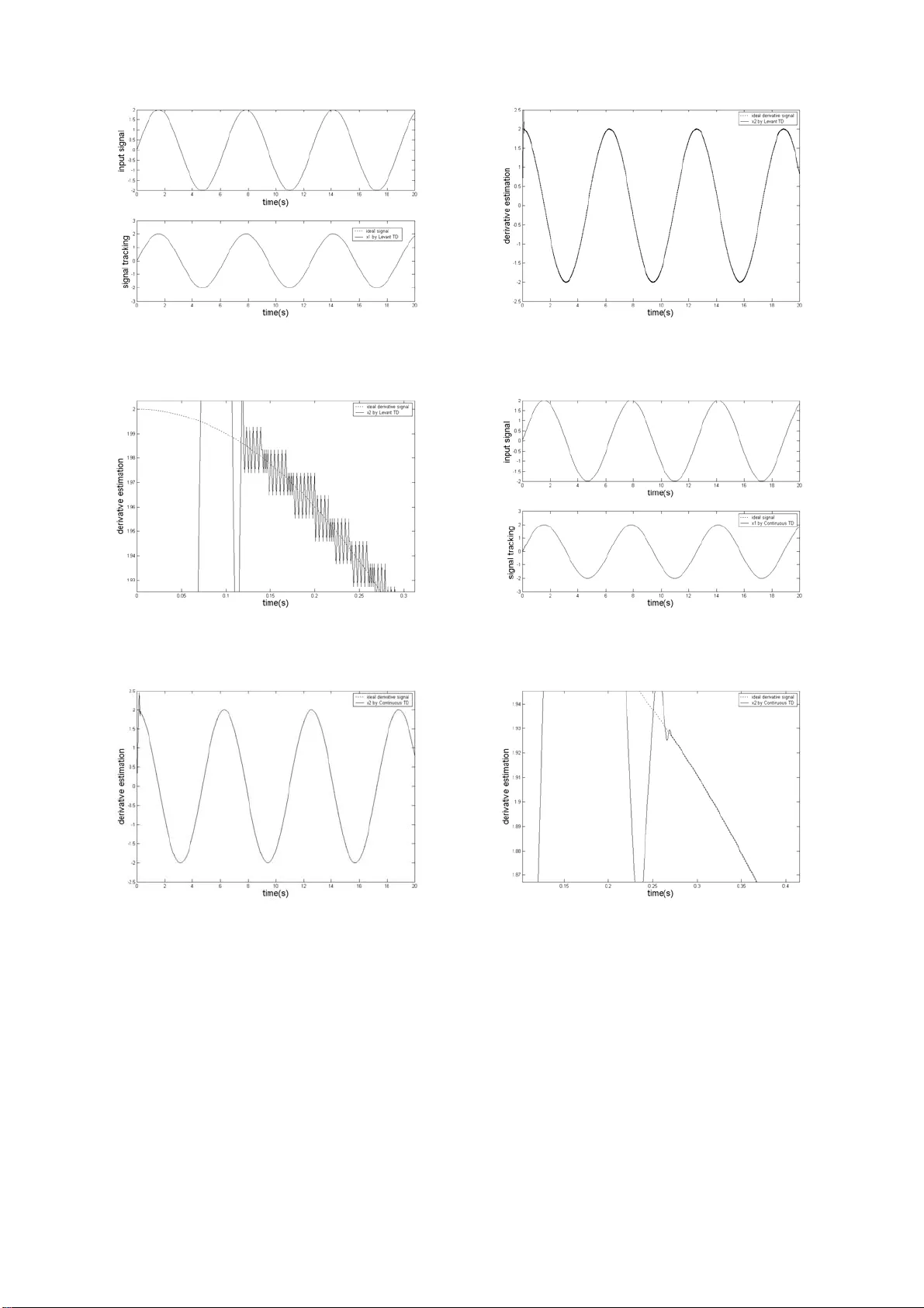
1 Design and analysis of continuous hybrid differ entiator Xinhua W ang and Hai Lin Department of Electrical & Computer E ngineer ing, National University of Singapore, 4 Engineer ing Drive 3, Singapore 1 17576 E-mail: wangxinhua04@gmail.com Abstract: In this paper , a continuous hybrid dif ferentiator is presented based on a strong L yapunov function. The dif ferentiator design can not only reduce suf ficiently chattering phenome non of derivative estimation by introducing a perturbation parameter , but also the dynamical perform ances are improved by adding linear correction terms to th e nonlinear ones. Moreov er , strong robustness ability is obtained by integrating sliding mode items and the linear filter . Frequency analysis is applied to compare the hybrid continuous dif ferentiator with s liding mode dif ferentiator . The merits of the continuous hybrid dif ferentiator include the excellent dynamical performances, restrain ing noises suf ficiently , and avoiding the chattering phenomenon. Keywords: continuous hybrid, dif ferenti ator , frequency analysis. 1. Introduction Diff erentiation of signals is a well -known problem [1-6], which has attr acted m uch attention in rece nt years. Obtaining the velocities of tracked targets is crucial for several kinds of systems with correct and timely performances, such as the m issile-interception systems [7] and underwater vehicle systems [8], in which disturbances must be restrained. The simple r ealization and robustness of dif ferentiators should be taken into consideration . The high-gain dif ferentiators [4, 19, 22] provide for an exact derivative when their gains tend to infinity . Unfortunately , their sensitivity to small high-f requency noi se also infinitely grows. W ith any finite gain values such a dif ferentiator has also a finite bandw idth. Thus, being not exact, it is, at the sam e time, insensitive with respect to high-frequency noise. Such insensitivity m ay be considered both as advantage 2 or disadvantage depending on the circumstances. More over , high gain results in peaking phenomenon. In [5, 6], a dif ferentiator via sec ond-order (or high-order) sliding modes algorithm has been proposed, and its frequency characteristics is given in [26]. The information one needs to know on the signal is an upper bound for Lipschitz consta nt of the derivative of the signal. Although second -order sliding mode is introduced and there exists no chattering phenomenon in signal tracking. However , for the robust exact dif ferentiator , in the second dynamical equation, a sw itching function exists. The output of derivative estimation is continuous but not sm ooth. Therefore, chattering phenomenon still exists in derivative estimation. In [28, 29], a switching f unction is designed to switc hes between the robust ex act dif ferentiator and a standard lead filter so as to re nder the error system uniform ly globa lly exponentially practically stable without considering the existence of noises. Thus a global robust exact di ff erentiator (GRED) is integrated. The switching function is decided by the outputs error of the two dif ferentiators and som e given parameters. Wh en noises exist in signal, th e exact derivative estim ation cannot be obtain ed by these two diff erentiators independently or by GRED. It is di fficult to select these param eters of the switching function when noises exist. Moreover , though no ch attering phenomenon happens for signal tracking, it still exists in derivative estima tion because of discontinuous functio n in the second equation of robust exact dif ferentiator . In [18], we presented a finite-tim e-conver gent differentiator based on finite-time stability [15-17] and singular perturbation technique [9-14] . However , the differentiators in [18] are complicated. In [20], we designed a hybrid dif ferentiator with high speed conver gence, and it succeeds in applications to velocities estimation for low-speed regions only based on positi on m easurements [21] and to velocities estim ation for a quadrotor aircraft [27], in which only the conver gence of signa l tracking was described for this dif ferentiator , but the convergence of derivativ e estimation was not given, and the regulation of 3 parameters has no rules. Moreover , the proposed di fferentiator requires the boundedness of the first-order and second-order derivatives of the input signal. From the previous analysis of linear differentiators [4, 19, 22] and sliding mode differentiators [5, 6], the linear differentiato r and the nonlinear differ entiato r, two notable differences can be observed. First, the two algorithms have quite diffe rent converging properties: the lin ear system converges exponentially, whereas the trajectories of the slid ing mode algorithm converge in finite tim e. This is due to the lack of local Lipschitzness of the SO SM algorithm at the origi n, that is, its behavior ar ound the zero state is very strong compared to the linear case. On the other side, the linear co rrection term s are stronger than the ones of the sliding mode algorithm far from the origin. These differences cause another striking difference between both algorithms: th e kind of perturbations that each one is able to tolerate. The m ain difference is that the linear system can deal with perturbations that are stronger very far from the origin and weaker near the origin than the ones that are e ndured by the sliding mode algorithm. So, for example, the sliding mode algorithm is not able to endure (globally) a bounded perturbation with linear growth in time, but the linear algorithm can deal with it easily. However, the linear algorithm is not able to support a strong perturbation near the origin, what is one of the main advantages of the sliding mode. In this paper , in order to integrate the merits of linear dif ferentiator and robus t exact dif ferentiator , and to restrain their shortcom ings respectively , a continuous hybrid dif f erentiator algorithm is presented based on strong L yapunov function. The proposed differentia tor is an integrati on of a nonlinear term (comprising of continuous power function) and a linear correction term. The overall design is an extension of the second order dif ferentiators proposed by Arie Levant [5, 6] in that a perturbation parameter α is introduced which takes values (0,1) and an addition al linear correction term is appended, so that it inherits the best prope rties of both. The switching function in the second equation of robust exact dif ferentiator is substituted by a continuou s power function with a perturbation parameter . Therefore, 4 chattering phenomenon can be avoided in the output of derivative estim ation. St rong robustness ability by L yapunov function is obtained by integrating sliding m ode items and the linear f ilter . The linear part can restrain high-frequency noises by gi ving a suitable nature frequenc y , and small bounded noises can be restrained by the sliding m ode items, at the same tim e, the sliding m ode items can compensate the delay brought by the linear filter . Moreov er , the proposed cont inuous hybrid diff erentiator only requires the boundness of the second-order deri vative of the input signal. A frequency response method, describing function me thod [13, 23], can be used to approximately analyze and predict nonlinear behavi ors of dif ferentiators. Frequency analysis is applied to compare hybrid continuous dif ferentiator with sliding mode diff erentiator . Moreover , the advantage of the use of Lyapunov functions is that it is possible to obtain explicit rela tions for the design parameters. 2. Prelim inaries First of all, the concepts related to finite -time control are given. Definition 1 [16]: Consider a time-invariant system in the form of ( ) ( ) ,0 0 , n x fx f x R == ∈  ( 1 ) where 0 ˆ : n f UR → is continuous on an open neighborhood 0 ˆ U of the origin. The equilibrium 0 x = of the system is (locally) finite-tim e stable if (i) it is asym ptotically stable, in ˆ U , an open neighborhood of the origin, with 0 ˆˆ UU ⊆ ; (ii) it is finite-time conver gent in ˆ U , that is, for any initial condition { } 0 ˆ \0 xU ∈ , there is a settling tim e 0 T > such that every solution ( ) 0 , x tx of system (1) is defined with ( ) { } 0 ˆ ,\ 0 xt x U ∈ for [] 0, tT ∈ and satisfies ( ) 0 lim , 0 tT xtx → = ( 2 ) and x ( t , x 0 )=0, if t  T . Moreover , if ˆ n UR = , the origin 0 x = is globally finite-tim e stable. Definition 2 [31, 32, 33]: A family of dilations δ ρ r is a mapping that assigns to every real 0 ρ > a dif feomorphism 5 () ( ) 1 11 ,, ,, n r r r nn x xx x ρ δρ ρ = "" ( 3 ) where 1 , n x x " are suitable coordinates on n R and ( ) 1 ,, n rr r = " with the dilation coefficients 1 , n rr " positive real numb ers. A vector field f ( x )=( f 1 ( x ),  , f n ( x )) T is homogeneous of degree k  R with respect to the family o f dilations δ ρ r if () ( ) 1 1 ,, , 1 ,, , 0 ni rr k r in i fx x f x i n ρρ ρ ρ + = => "" ( 4 ) System (1) is called homogeneous if its vector field f is homogeneous. The following lemma was presented in some references like [15, 17, 24, 25]. Lemma1 [15, 24, 25] : Suppose that system (1) is homogeneous of degree k <0 with respect to the family of dilations δ ρ r , f ( x ) is continuous and x =0 is its asymptotically stable equilibrium. Then equilibrium of system (1) is globally finite-time stable. Lemma 2 [17]. Suppose the origin is a finite-time-stable equilib rium [17, Theorem 4.3] of (1), and the settling-time function T f is continuous at zero, where f ()is continuous. Let N be defined as in Definition 1 and let θ  (0,1). Then there exists a continuous scalar function V such that 1) V is positiv e definite and 2) d V /d t is real valued and continuous on N and there exists c >0 such that 0 ≤ + θ cV V  , for any ( ) 1 , 0 ∈ θ ( 5 ) Assumption 1. For (1), there exist ( ] 0, 1 ρ ∈ and a nonnegative constant a such that () () 11 ii f zf z a z z ρ −≤ − ( 6 ) where , n zz ∈ℜ . Remark 1. There are a number of nonlinea r functions actually satisfying assumption 2. For example, one such function is ρ x since ( ] 1 , 0 , 2 1 ∈ − ≤ − − ρ ρ ρ ρ ρ x x x x . Moreover, there are smooth functions also satisfying this property. In fact, it is easy to verify that ρ x x x x − ≤ − 2 sin sin for any ( ] 1 , 0 ∈ ρ . 3. Problem statement 6 A. Robust exact dif ferentiator [5, 6] In [5, 6], a finite-time convergent dif ferentiator ba sed on second-order sliding is presented as follow: () () () () () 1 2 11 12 2 11 11 12 1 11 sgn sgn x xx v t x v t xx v t λ λ =− − − =− −   ( 7 ) where the second-order dif ferentiable signal ( ) vt is bounded, and ( ) 2 vt L ≤  , 2 L is a positive consta nt, 12 ,0 λ λ > , 12 L λ > . For dif ferentiator (7), from Lemma 1, there exists a time 0 s t > such that ( ) ( ) 11 12 , x vt x vt ==  ( 8 ) for s tt ≥ . Moreover , let () vt is the input signal w ith noise, ( ) 0 vt is the desired signal, and it is sa tisfied with ( ) ( ) 0 vt v t ε −≤ . Therefore, for som e positive constants i μ , 0, 1 i = , the following inequalities are established [6]: () 2 2 1, 1 1, 1 0 ,0 , 1 i i ii i ex v t i με − ++ =− ≤ = ( 9 ) In robust exact dif ferentiator (7), though the output x 11 is smooth, the chatte ring phenomenon exists in the output x 2 because the discontinuous sgn( ) exists in th e second dif ferential equation of diff erentiator (7). In the motor velocity fee dback systems, the chattering in x 12 can make motors trem bling. Therefore, chattering phenomenon must be rest ra ined suf ficiently in the output x 12 for a dif ferentiator . In the following, we analyse dif ferentiator (7 ) from its frequency characteristics. A.1 Frequency characteristics of r obust exact dif ferentiator (7) Let () 11 11 sin ex v t A t ω =− = , we have () 0.5 1.5 0.5 0 0 22 sin sgn sin sin sin AA d t A d t π π ω τω τ ω τ ω ω τ ω ππ = ∫∫ ( 1 0 ) W e can get 0 24 sin dt π ωτ ω π π = ∫ and () 2 0 2 sin 1 dt π ωτ ω π = ∫ . In (10), let 1.5 0 2 sin dt π ω τω π Ω= ∫ , therefore, we have 14 π < Ω< . The describing function of nonlinear function () 0.5 sgn is () 0.5 NA A =Ω , and the linearization system of dif ferentiator (7) is 7 () () () () 11 12 2 11 0.5 12 1 11 4 x xx v t A xx v t A λ λ π Ω =− − =− −   ( 1 1 ) The nature frequency of system (1 1) is 1 0.5 2 n A λ ω π = ( 1 2 ) and its damping coef ficient is 2 1 4 λ π ς λ Ω = ( 1 3 ) From (1 1), (12) and (13), we can fi nd that when the tracking error is lar ge, i.e., far from the origin, the gains in (1 1) are small. On the other hand, when th e tracking error is small, i.e., around the origin, the gains are large. Therefo re, the beha vior of robust exact di f ferentiator is weak far from the origin, and contrarily , the behavior ar ound the origin is strong. A.2 Analysis of chattering phenomenon for r obust exact differ entiator (7) In the following, we give two examples to expl ain the chattering phenom enon in sliding control systems. Example 1: First-order systems 1) First-order sliding mode system: () 1 1 2s g n xu ux = =−  ( 1 4 ) 2) First-order lin ear system : 2 2 2 yu uy = = −  ( 1 5 ) 3) First-order continuous nonlinear system (with a power function): () 3 0.5 3 2s g n zu uz z = =−  ( 1 6 ) The simulation curves of the three sy stems are shown in Figures 1-3. 8 Fig. 1 x , y and z Fig. 2 The magnified figure of Fig. 1 Fig. 3 u 1 , u 2 and u 3 From Fig. 2, we can find that chattering phenomenon happen in system (14). And there is no chattering phenomenon in system (16). Example 2: Second-order systems: 1) Second-order sliding mode system: () () 1 2 12 1 1 1 1 22 1 sgn sgn x xk x x xk x =− =−   ( 1 7 ) 2) Second-order linear system: 12 1 1 22 1 y yk y y ky = − =−   ( 1 8 ) 3) Second-order continuous nonlinear system: 9 () () 1 2 12 1 1 1 22 1 1 sgn sgn zz k z z zk z z α α + =− =−   , ( ) 12 0, 1 , , 0 kk α ∈ > ( 1 9 ) For second-order continuous non linear system (19), selectin g a L yapunov function as follow () 2 1 1 2 2 2 12 1 1 1 2 2 11 sgn 12 2 k Vz z k z z z α α α + + ⎛⎞ =+ + − ⎜⎟ + ⎝⎠ ( 2 0 ) W e can get that {} () () {} {} () 1 31 21 min min 21 min PQ VV P α α α α λλ λ − + + + ≤−  ( 2 1 ) and () 31 01 21 α α + < < + ( 2 2 ) where 2 2 11 1 4 1 1 2 2 k kk P k α ⎡⎤ +− ⎢⎥ = + ⎢⎥ − ⎣⎦ , ( ) ( ) () () 2 21 1 1 1 21 1 11 2 kk k k Q k αα αα ⎡ ⎤ ++ − + = ⎢ ⎥ −+ + ⎣ ⎦ ( 2 3 ) Therefore, we know that system (19) is finite time stable. 4) Second-order continuous hybrid system: () () 1 2 12 1 1 1 3 1 22 1 1 4 1 sgn sgn ww k w w k w wk w w k w α α + =− − =− −   , ( ) 12 34 0, 1 , , , 0 kk k k α ∈ > ( 2 4 ) For second-order continuous non linear system (24), selectin g a L yapunov function as follow () 2 1 1 22 3 2 14 1 2 1 1 1 2 1 2 2 11 sgn 12 2 k Vw k w w k w w k w w α α α + + ⎛⎞ =+ + + + − ⎜⎟ + ⎝⎠ ( 2 5 ) W e can get that { } {} { } {} min 1 min 2 0.5 max max VV V λλ λ λ ΩΩ ≤− − Π Π  ( 2 6 ) where 10 ( ) ( ) ( ) () () () () ( ) () 2 21 1 2 1 14 3 3 13 21 0 1 02 5 3 2 13 1 kk k k kk k kk αα αα αα α ⎡⎤ ++ − + ⎢⎥ ⎢⎥ Ω= + + − + ⎢⎥ −+ − + + ⎢⎥ ⎣⎦ , ( ) ( ) () 2 23 2 23 4 3 3 3 20 0 0 01 kk kk k k k α ⎡⎤ ++ ⎢⎥ ⎢⎥ Ω= + − ⎢⎥ − ⎢⎥ ⎣⎦ , () 2 13 1 2 13 4 3 3 13 4 1 2 2 k kk k kk k k k kk α ⎡ ⎤ ⎛⎞ − ⎜⎟ ⎢ ⎥ + ⎝⎠ ⎢ ⎥ ⎢ ⎥ Π= + − ⎢ ⎥ ⎢ ⎥ −− ⎢ ⎥ ⎣ ⎦ ( 2 7 ) Therefore, we know that system (24) is finite time stable. Parameters: 123 4 6, 9, 10, 20, 0. 2 kk k k α == = = = . The simulation curves of the four system s are shown in Figures 4-6. Fig. 4 x 1 , y 1 , z 1 and w 1 F i g . 5 x 2 , y 2 , z 2 and w 2 Fig. 6 The m agnified figure of Fig. 5 W e can find that though x 1 is smooth, there ex ists chatte ring phenom enon in the output x 2 of system (17), because a switching function exists in the sec ond equation of system (17). Therefore, for the robust 11 exact dif ferentiator (7), which ha s the same structure with syst em (17), chattering phenomenon in derivative estimation is inevitable. Moreover , no chattering phenomenon exist in the outputs of continuous nonlinear system (19) and continuous hybrid system (24), and the behavior of system (24) is better . B. Linear high-gain dif ferentiator [4, 19, 22] For linear high-gain dif ferentiator () () () () 1 21 22 21 2 22 21 2 a x xx v t a xx v t τ τ ⎧ =− − ⎪ ⎪ ⎨ ⎪ =− − ⎪ ⎩   ( 2 8 ) we know that [4, 19, 22] 21 22 00 lim 0, lim 0 xx ττ →→ = = ( 2 9 ) where 12 ,0 aa > . B.1 Frequency characteristics of lin ear high-gain dif feren tiator (28) In the following, we will an alyse the ability of re stra ining noises for the linear d if ferentiator (28). Laplace transformation of system (28) is () () () () () () () () () 1 21 22 21 2 22 21 2 a s Xs X s Xs V s a sX s X s V s τ τ =− − =− − ( 3 0 ) where () 21 X s , () 22 X s and ( ) Vs are respectively Laplace trans formations of () 21 x t , ( ) 22 x t and () vt . Therefore, we have the tran sfer function of signal tracking () () 12 2 21 2 12 2 aa s Xs aa Vs ss ττ τ τ + = ++ ( 3 1 ) and the transfer function of derivative estimation 12 () () 2 2 22 2 12 2 a s Xs aa Vs ss τ τ τ = ++ ( 3 2 ) Then, the nature frequency n ω is 2 n a ω τ = ( 3 3 ) and the damping coef ficient ξ is satisfied with 1 2 2 a a ξ = ( 3 4 ) For the transfer function (31) and (32), let sj ω = , respectively we have () ( ) () 21 20 lg 0 Xj L Vj ω ω ω =≈ as n ω ω  ( 3 5 ) () ( ) () 21 20 lg 4 0 lg n Xj L Vj ω ω ω ω ω =≈ − as n ω ω  ( 3 6 ) and () ( ) () 22 20 lg 20 l g d Xj L Vj ω ω ω ω =≈ as n ω ω  ( 3 7 ) () ( ) () 22 20 lg 20 l g 20 lg 20 lg n dn n n Xj L Vj ω ω ω ωω ω ω ω ω =≈ = − as n ω ω  ( 3 8 ) From the analysis above, linear dif ferentiator can restrain high-frequency noises under the condition that τ should be selected a suitable va lue, but not a suff iciently small value. In the following, we will analyse the convergence of linear dif feren tiator (28 ) by selecti ng finite parameter τ . B. 2 convergence of linear differ entiator (28) by finite parameter τ Let ( ) ( ) 21 21 22 22 , e x vt e x vt =− = −  ( 3 9 ) then we have the error system as follow: 13 ( ) eA e B v t =+   ( 4 0 ) where 1 2 2 1 0 , 1 0 a AB a τ τ ⎡⎤ − ⎢⎥ ⎡ ⎤ == ⎢⎥ ⎢ ⎥ − ⎣ ⎦ ⎢⎥ − ⎢⎥ ⎣⎦ ( 4 1 ) The solution trajectory of the error system is: () ( ) () 0 0 t At At et e e e B d η η − =+ ∫ ( 4 2 ) There exist positive constants 1 , λ σ , such that () () () 12 0 0 t t At et e e L e d λ η τ σ η − − ≤+ ∫ ( 4 3 ) Moreover , the following inequality is satisfied: () () () 11 2 0 0 tt t et e e L e d λλ η ττ σ ση −− − ≤+ ∫ ( 4 4 ) Therefore, we have () () 12 1 01 tt L et e e e λλ ττ τσ σ λ −− ⎛⎞ ≤+ − ⎜⎟ ⎝⎠ ( 4 5 ) Therefore, () 21 2 12 lim t n aL L et σ τσ λ ωλ →∞ ≤= ( 4 6 ) From the analysis above , in order to m ake ( ) et sufficiently sm all, parame ter τ should be selected suf ficiently small. However , suitable nature frequency n ω should be selected in order to restrain high-frequency noises. Therefore, parameter τ cannot be sufficiently small. Thus this linear dif ferentiator exists a sta tic error decided by the selection of parameter τ . For linear diff erentiator (28), we also find that when th e tracking error is lar ge, i.e., far from the origin, its behavior is strong. On the other hand, when tracki ng error is small, i.e., ar ound the origin, its behavior is weak. 14 In general, we want to have the two abilities of linear high-gain differ entiator and robust exact dif ferentiator . In the following, we will introduce a global robust ex act dif ferentiator , which use a switching function to switch between the two dif ferentiators. C. Global robust exact dif ferentiator (GRED) For the following GRED [28, 29] () () () () () 1 2 11 12 0 11 11 12 1 11 sgn sgn x xx v t x v t xx v t λ λ ⎧ =− − − ⎪ ⎨ ⎪ =− − ⎩   , () () () () 1 21 22 21 2 22 21 2 a x xx v t a xx v t τ τ ⎧ =− − ⎪ ⎪ ⎨ ⎪ =− − ⎪ ⎩   ( 4 7 ) The position tracking output 1 y and derivative estimation output 2 y are respectiv ely ( ) ( ) ( ) 11 2 1 1 1 1 1 pp ye x e x αα =+ − ( 4 8 ) ( ) ( ) ( ) 22 2 2 2 1 2 1 dd ye x e x αα =+ − ( 4 9 ) where 11 21 p exx = − , 12 22 d ex x = − () 1 0, , 1, pp p pp p pp p p p p pp ec ec ec e c e ε ε α εε ε ⎧ <− ⎪ ⎪ −+ ⎪ =− ≤ < ⎨ ⎪ ⎪ ≥ ⎪ ⎩ , () 2 0, , 1, dd d dd d dd d d d d dd ec ec ec e c e ε ε α εε ε ⎧< − ⎪ −+ ⎪ = −≤ < ⎨ ⎪ ⎪ ≥ ⎩ ( 5 0 ) p c and d c are the boundary layers respectively used to smoothen the switching functions of signal tracking and derivative estimation, and , pp d d KK ε τε τ = = with p k and d k being the appropriate positive design param eters. Due to the existence of noises, the outputs of line ar differentiator and robust ex act differentiator are all not exact. From (9) and (46), we get 12 11 21 11 21 11 21 0 p L ex x e e e e τ σ με λ =− = −≤ + ≤ + ( 5 1 ) 1 12 2 12 22 12 22 12 22 1 d L ex x e e ee τσ με λ =− = −≤ + ≤ + ( 5 2 ) It is dif ficult to select the parameters p k and d k when noises exist in signal. It may cause the 15 switching function invalid to switches between the two dif ferentiators. Moreover , though no chattering phenomenon happens for signal tracki ng, it still exists in derivative estimation because of discontinuous function in the second equation of robust exact dif ferentiator . In the following, we will present a continuou s hybrid dif ferentiator based on a strong L yapunov function. The dif ferentiator design can not only reduce suf ficiently chattering phenome non of derivative estimation, but also its dynamical perform ances ar e improved by adding linear correction terms to the nonlinear ones. Moreover , the robustness will be given by L yapunov function method. 4. Hybrid continuous nonlinear differ entiator A. Convergence of hybrid continuous nonlinear dif ferentiator The hybrid continuous differen tiator is given as follow: () () () () () () () () () () 1 2 12 1 1 1 2 1 23 1 1 4 1 sgn sgn x xk x v t x v t k x v t x k x vt x vt k x vt α α + =− − − − − =− − − − −   ( 5 3 ) Theorem 1: For continuous hybrid dif ferentiator (53) and bounded second-order diff erentiable signal ( ) vt , there exist constants 0 i k > ( 1, , 4 i = " ) , 0 s t > and 01 α < < such that {} () () 1 2 21 m i n 1 22 L α α ςλ + ≤Γ Ω ( 5 4 ) for s tt ≥ . Where ( ) 2 vt L ≤  , and () 1 2 11 1 2 sgn ee e e α ς Τ + ⎡⎤ = ⎢⎥ ⎣⎦ , ( ) 11 ex v t =− , ( ) 22 ex v t =−  , [ ] 11 2 2 kk Γ =− ( 5 5 ) () ( ) ( ) () () () () ( ) () 2 31 1 2 1 14 2 2 12 21 0 1 02 5 3 2 13 1 kk k k kk k kk αα αα αα α ⎡⎤ ++ − + ⎢⎥ ⎢⎥ Ω= + + − + ⎢⎥ −+ − + + ⎢⎥ ⎣⎦ ( 5 6 ) In fact, { } () 2m i n 1 2 1 L λ ΓΩ < can be obtained in diff erentiator (53) and 0< α <1 is selected suf ficiently small, ( α +1)/(2 α ) is suf ficiently lar ge, therefore, || ζ || 2 becomes suf ficiently in a finite time. This will be given in the following proof. Proof: Let 16 ( ) ( ) 11 2 2 , ex v t e x v t =− = −  ( 5 7 ) The error system is () () ( ) 1 2 12 1 1 1 2 1 23 1 1 4 1 sgn sgn eek e e k e ek e e k e v t α α + =− − =− − −    ( 5 8 ) The L yapunov function is selected as () 2 1 1 22 3 2 14 1 21 1 1 2 1 2 2 11 sgn 12 2 k Ve k e e k e e k e e α α α + + ⎛⎞ =+ + + + − ⎜⎟ + ⎝⎠ ( 5 9 ) Therefore, we have V ς ς Τ = Π ( 6 0 ) where () 1 2 11 1 2 sgn ee e e α ς Τ + ⎡⎤ = ⎢⎥ ⎣⎦ , () 3 12 1 2 12 4 2 2 12 4 1 2 2 k kk k kk k k k kk α ⎡ ⎤ ⎛⎞ − ⎜⎟ ⎢ ⎥ + ⎝⎠ ⎢ ⎥ ⎢ ⎥ Π= + − ⎢ ⎥ ⎢ ⎥ −− ⎢ ⎥ ⎣ ⎦ ( 6 1 ) Moreover , it satisfies {} {} 22 min max 22 V λς λ ς Π≤ ≤ Π ( 6 2 ) where 21 22 11 2 2 ee e α ς + = ++ ( 6 3 ) The time derivative along the trajecto ries of the hybrid differentiator is () 1 2 11 2 1 Ve v t α ς ςς ς ς − ΤΤ =− Ω − Ω + Γ   ( 6 4 ) where ( ) ( ) ( ) () () () () ( ) () 2 31 1 2 1 14 2 2 12 21 0 1 02 5 3 2 13 1 kk k k kk k kk αα αα αα α ⎡⎤ ++ − + ⎢⎥ ⎢⎥ Ω= + + − + ⎢⎥ −+ − + + ⎢⎥ ⎣⎦ , ( ) ( ) () 2 32 2 22 4 2 2 2 20 0 0 01 kk kk k k k α ⎡ ⎤ ++ ⎢ ⎥ ⎢ ⎥ Ω= + − ⎢ ⎥ − ⎢ ⎥ ⎣ ⎦ , [ ] 11 2 2 kk Γ= − ( 6 5 ) Therefore, we have {} {} 1 22 2 1 min 1 min 2 2 1 22 2 2 Ve L α λ ςλ ς ς − ≤− Ω − Ω + Γ  ( 6 6 ) From (63) and 0< α <1, we have 17 11 21 1 2 e αα α ς − − + ≥ ( 6 7 ) Therefore, from (67), inequali ty (66) can be written as {} {} 1 22 1 min 1 mi n 2 2 1 22 2 2 2 VL α α λ ςς λ ς ς − + ≤− Ω − Ω + Γ  ( 6 8 ) Therefore, we have {} {} 2 2 1 min 1 2 1 min 2 22 2 2 VL α α λς ς λ ς + ⎛⎞ ≤− Ω − Γ − Ω ⎜⎟ ⎝⎠  ( 6 9 ) From (62), we get {} {} 2 2 max min VV ς λλ ≤≤ Π Π ( 7 0 ) Therefore, we have {} {} { } {} 0.5 2 min 2 1 min 1 2 1 22 max max V VL V α α λ λς λ λ + Ω ⎛⎞ ≤− Ω − Γ − ⎜⎟ Π ⎝⎠ Π  ( 7 1 ) If {} 2 1 min 1 2 22 L α α λς + Ω> Γ , error system (58) is finite- time stable. Therefore, we have {} () 1 2 21 m i n 1 22 L α α ςλ + ≤Γ Ω ( 7 2 ) for s tt ≥ . In fact, we can select ,1 , , 4 i ki = " such that { } 21 m i n 1 2 1 L λ Γ Ω< . Because 01 α << is suf ficiently small, () ( ) 12 α α + is suf ficiently lar ge, 2 ς is suf ficiently small in a finite tim e.  For (66), we can find that when the tracking error is lar ge, i.e., far from the origin, {} 1 2 2 1m i n 1 2 e α λ ς − −Ω is small, and {} 2 min 2 2 λ ς −Ω is lar ge, therefore, the behavior of {} 2 min 2 2 λ ς −Ω is strong, and { } min 2 λ Ω is decided by the parameters 2 k and 4 k of linear part. On the other hand, around the origin, {} 1 2 2 1m i n 1 2 e α λ ς − −Ω is large, and {} 2 min 2 2 λ ς −Ω is small, so the behavior of {} 1 2 2 1m i n 1 2 e α λ ς − −Ω is strong. Therefore, the behaviors are strong during the whole conver gences. B. Robustness analysis for hybrid continuous dif ferentiator Theorem 2: For hybrid dif ferentiato r (53), if there exis t a noise in signal ( ) vt , i.e., () ( ) ( ) 0 vt v t t δ =+ , where ( ) 0 vt is the desired second-or der derivable signal, and ( ) t δ is a bounded noise and is satisfied with ( ) t δ ε ≤ , then, the following inequality is establishe d in finite time 18 ( ) {} ( ) {} 12 2 min 1 2 1 min 2 2 max , L εε ς λλ ⎧⎫ ΨΨ ⎪⎪ ≤ ⎨⎬ Ω− Γ Ω ⎪⎪ ⎩⎭ ( 7 3 ) where () ( ) 11 1 22 13 2 1 2 2 1 22 2 k kk k αα α ε εε −+ + ⎡⎤ ⎛ ⎞ Ψ= + Γ + ⎜⎟ ⎢⎥ ⎝⎠ ⎣⎦ () () () ( ) 11 1 22 24 2 2 1 2 2 3 4 22 22 1 2 kk k k k k αα αα ε εε ε ε −+ − ⎡⎤ ⎛⎞ Ψ= + Γ + + + Γ + ⎢⎥ ⎜⎟ ⎢⎥ ⎝⎠ ⎣⎦ ( ) ( ) ( ) () () () () ( ) () 2 31 1 2 1 14 2 2 12 21 0 1 02 5 3 2 13 1 kk k k kk k kk αα αα αα α ⎡⎤ ++ − + ⎢⎥ ⎢⎥ Ω= + + − + ⎢⎥ −+ − + + ⎢⎥ ⎣⎦ , ( ) ( ) () 2 32 2 22 4 2 2 2 20 0 0 01 kk kk k k k α ⎡ ⎤ ++ ⎢ ⎥ ⎢ ⎥ Ω= + − ⎢ ⎥ − ⎢ ⎥ ⎣ ⎦ , [ ] 11 2 2 kk Γ= − , [ ] 21 2 1 kk Γ =− , ( ) 02 vt L ≤  ( 7 4 ) Proof: Let ( ) ( ) 11 0 2 2 0 , ex v t e x v t =− = −  ( 7 5 ) The error system is () () ( ) 1 2 12 1 1 1 2 1 2 23 1 1 4 1 4 0 sgn sgn eek e e k e k ek e e k e k v t α α δδ δ δδ δ + =− − − − + =− − − − + −    ( 7 6 ) Let () () () () 11 22 11 1 1 1 21 1 1 1 sgn sgn sgn sgn ee e e ee e e αα αα δδ δδ ++ Δ= − − − + Δ= − − − + ( 7 7 ) Therefore, from Assumption 1 and Remark 1, we have 11 1 1 22 2 2 1 11 2 22 22 αα α α α αα α δ ε δε − −+ + −− Δ≤ ≤ Δ≤ ≤ ( 7 8 ) The L yapunov function is selected as () 2 1 1 22 3 2 14 1 2 1 1 1 2 1 2 2 11 sgn 12 2 k V e ke e k e e ke e α α α + + ⎛⎞ =+ + + + − ⎜⎟ + ⎝⎠ ( 7 9 ) Therefore, we have V ς ς Τ = Π ( 8 0 ) 19 where () 1 2 11 1 2 sgn ee e e α ς Τ + ⎡⎤ = ⎢⎥ ⎣⎦ , () 3 12 1 2 12 4 2 2 12 4 1 2 2 k kk k kk k k k kk α ⎡ ⎤ ⎛⎞ − ⎜⎟ ⎢ ⎥ + ⎝⎠ ⎢ ⎥ ⎢ ⎥ Π= + − ⎢ ⎥ ⎢ ⎥ −− ⎢ ⎥ ⎣ ⎦ ( 8 1 ) Moreover , it satisfies {} {} 22 min max 22 V λ ςλ ς Π≤ ≤ Π ( 8 2 ) where 21 22 11 2 2 ee e α ς + = ++ ( 8 3 ) The time derivative of V along the solution of e rror system (76) is () ( ) () () ( ) [] () () () ( ) {} {} () 1 2 11 2 1 11 22 13 1 1 1 1 2 4 1 1 1 2 2 3 2 4 1 1 2 12 1 1 1 2 2 1 1 2 3 24 1 22 2 1 min 1 min 2 2 1 22 2 2 1 1 2 13 2s g n 2 1 1 2 1 2 Ve v t e k e e kk k e kk e k k k kk e k k k k k k k eL k ek α αα α α α ςς ς ς ς δδ δ α ς δδ δ λς λ ς ς α − ΤΤ −+ − − − =− Ω − Ω + Γ ⎡⎤ +Δ + + Δ + + Δ + ⎢⎥ ⎣⎦ + ⎧⎫ +− Δ + + Δ + − Δ + ⎨⎬ ⎩⎭ ≤− Ω − Ω + Γ + ++   () () ( ) 11 22 21 2 22 11 1 22 42 2 1 2 2 3 4 22 2 2 2 22 1 2 kk kk k k k k αα αα αα εε ς εε ε ε ς −+ −+ − ⎡⎤ ⎛ ⎞ Γ+ ⎜⎟ ⎢⎥ ⎝⎠ ⎣⎦ ⎡⎤ ⎛⎞ ++ Γ + + + Γ + ⎢⎥ ⎜⎟ ⎢⎥ ⎝⎠ ⎣⎦ ( 8 4 ) where ( ) () ( ) () () () () ( ) () 2 31 1 2 1 14 2 2 12 21 0 1 02 5 3 2 13 1 kk k k kk k kk αα αα αα α ⎡⎤ ++ − + ⎢⎥ ⎢⎥ Ω= + + − + ⎢⎥ −+ − + + ⎢⎥ ⎣⎦ , ( ) ( ) () 2 32 2 22 4 2 2 2 20 0 0 01 kk kk k k k α ⎡ ⎤ ++ ⎢ ⎥ ⎢ ⎥ Ω= + − ⎢ ⎥ − ⎢ ⎥ ⎣ ⎦ , [ ] 11 2 2 kk Γ= − , [ ] 21 2 1 kk Γ =− ( 8 5 ) Let () ( ) 11 1 22 13 2 1 2 2 1 22 2 k kk k αα α ε εε −+ + ⎡⎤ ⎛ ⎞ Ψ= + Γ + ⎜⎟ ⎢⎥ ⎝⎠ ⎣⎦ ( 8 6 ) () () () ( ) 11 1 22 24 2 2 1 2 2 3 4 22 22 1 2 kk k k k k αα αα ε εε ε ε −+ − ⎡⎤ ⎛⎞ Ψ= + Γ + + + Γ + ⎢⎥ ⎜⎟ ⎢⎥ ⎝⎠ ⎣⎦ ( 8 7 ) Therefore, the dif ferential inequa lity (84) can b e rewritten as 20 {} {} () () 11 22 22 1m i n 1 m i n 2 1 1 2 1 2 22 2 2 2 2 Ve e L αα λ ςλ ς ε ς ς ε ς −− ≤− Ω − Ω + Ψ + Γ + Ψ  ( 8 8 ) Suppose there exist positive constants 1 c and 2 c such that () 11 2 c ες Ψ< and ( ) 22 2 c ες Ψ< ( 8 9 ) Therefore, we have {} {} 1 22 2 1m i n 1 1 2 1 m i n 2 2 22 2 2 Ve c L c α λ ςς λ ς − ≤− Ω − + Γ − Ω − ⎡⎤ ⎡ ⎤ ⎣⎦ ⎣ ⎦  ( 9 0 ) From (83) and 0< α <1, we have 11 21 1 2 e αα α ς − − + ≥ ( 9 1 ) Therefore, we get {} {} {} {} 1 22 1 min 1 1 2 1 min 2 2 22 2 2 2 2 2 1 min 1 1 2 1 min 2 2 22 2 2 Vc L c cL c α α α α ς λς ς λ ς λς ς λ ς − + + ≤− Ω − + Γ − Ω − ⎡⎤ ⎡ ⎤ ⎣⎦ ⎣ ⎦ ⎧⎫ =− Ω − − Γ − Ω − ⎡⎤ ⎡ ⎤ ⎨⎬ ⎣⎦ ⎣ ⎦ ⎩⎭  ( 9 2 ) And from (82), we get {} {} 2 2 max min VV ς λλ ≤≤ Π Π ( 9 3 ) Therefore, {} {} {} {} 0.5 2 1 min 1 1 2 1 min 2 2 22 max max VV Vc L c α α λς λ λ λ + ⎧⎫ ≤− Ω − − Γ − Ω − ⎡⎤ ⎡ ⎤ ⎨⎬ ⎣⎦ ⎣ ⎦ Π ⎩⎭ Π  ( 9 4 ) If {} 1 2 21 2 2 min 1 1 L c α α ς λ + ⎛⎞ Γ > ⎜⎟ ⎜⎟ Ω− ⎝⎠ and { } min 2 2 c λ Ω > ( 9 5 ) the dif ferential inequality (94) is finite time conver gent, an d the error system (76) is finite-tim e stable. Because α is suf ficiently sm all, we want {} 1 2 21 2 min 1 1 L c α α λ + ⎛⎞ Γ ⎜⎟ ⎜⎟ Ω− ⎝⎠ also to be suf ficiently small, therefore, it is required that {} 21 2 min 1 1 01 L c λ Γ << Ω− . Then, we have { } 1m i n 1 2 1 2 cL λ <Ω − Γ and { } 2m i n 2 c λ < Ω ( 9 6 ) Therefore, from (89), we know that if 21 () {} 1 2 min 1 2 1 2 L ε ς λ Ψ > Ω− Γ and ( ) {} 2 2 min 2 ε ς λ Ψ > Ω ( 9 7 ) the dif ferential inequality (87) is finite tim e convergent. Therefore, we can get ( ) {} ( ) {} 12 2 min 1 2 1 min 2 2 max , L εε ς λλ ⎧⎫ ΨΨ ⎪⎪ ≤ ⎨⎬ Ω− Γ Ω ⎪⎪ ⎩⎭ ( 9 8 ) This concludes the proof.  Remark 2: The hybrid continuous dif ferentiato r (53) consists of the linear and nonlinear dif ferentiators given respectively as follow: ( ) ( ) () () 12 2 1 24 1 x xk x v t xk x v t =− − =− −   ( 9 9 ) and () () () () () () 1 2 12 1 1 1 23 1 1 sgn sgn x xk x v t x v t xk x v t x v t α α + =− − − =− − −   (100) In the following, we will give a theorem a bout continuous nonlinear dif ferentiator (100). Remark 3: When 0 α = , we can get a hybrid discontinuous dif ferentiator as follow: () () () () () () () () () 1 2 12 1 1 1 2 1 23 1 4 1 sgn sgn x x k x vt x vt k x vt x k xv t k xv t =− − − − − =− − − −   (101) and can get that ( ) ( ) 12 , x vt x vt ==  (102) For s tt ≥ . If the L yapunov function () 2 1 1 22 3 2 14 1 2 1 1 1 2 1 2 2 11 sgn 12 2 k Ve k e e k e e k e e α α α + + ⎛⎞ =+ + + + − ⎜⎟ + ⎝⎠ (103) is selected, we have the above conclusion. For linear dif ferentiator (99), it is required that k 2 and k 4 are selected suf ficiently large. In th e dif ferentiator (101), a discontinuous switching function sgn( ) exists in the second equation, therefore, there is chattering phenomenon in the output x 2 although x 1 is smooth. When high- frequency noises exist in the signal, this chattering can magni fy high-frequency noises around the origin. 22 5. Frequency analysis of hybrid differ entiator The linearization of hybrid co ntinuous dif ferentiator (5 3) by describing function is () () () () () 1 2 12 1 1 21 1 23 2 4 1 x xk A k x v t xk A k x v t α α ρ ρ − − ⎛⎞ =− + − ⎜⎟ ⎝⎠ =− + −   (104) The nature frequency of system (150) is 32 4 1 n k k A α ρ ω − = + (105) and the damping coef ficient is 1 2 11 2 1 32 4 2 kA k kA k α α ρ ς ρ − − + = + (106) In the hybrid nonlinear dif ferentiator (53), k 4 can be selected relatively sm all, and the normal nature frequency is relatively small too. The nonlinear item k 3 ρ 2 / A 1- α is the eff ective compensation to the linear part, i.e., the sliding mode item s can compensate the delay brought by the linear filter . When the magnitude of tracking error magnitude A is relatively larg e, because 0<1- α <1, A 1- α decreases, and ω n increases. When A is relatively sm all, ω n becomes sm all too, chattering and sm all high-frequency noises can be reduced. Better dynamic characteristic is obtained. 6. Simulations In the following sim ulations, we select the function of 2sin( t ) as the desired signal 0 v ( t ). 1) Derivative estimation without noise A. For Levant dif ferentiator (7), the param eters are λ 2 =6, λ 1 =28. Figures 7 and 8 show respectively simulation results of signal tracki ng and derivative estimation by robust exact dif ferentiator without noise. 23 Fig. 7 Signal tracki ng by robust exa ct diff erentiator Fig. 8-a Derivat ive estimation by robust exact differe ntiator Fig. 8-b The magnified figure of Fig. 8-a Fig. 9 Signal tracking by hybrid differenti ator Fig. 10-a Derivative estimation by hy brid dif ferentiator Fig. 10-b The m agnified figure of Fig. 9-a From the simulations above, we find that the o bvious chattering phenomenon happens in robust exact dif ferentiator . B. For hybrid dif ferentiator , figures 9 and 10 show respectively the simulation results of signal tracking and derivative estimation by hybrid dif ferentiator without noise. From the sim ulations above, chattering phenomenon is reduced suf ficiently and rapid a nd high-precision tracking can be guaranteed by 24 continuous dif ferentiator . 2) Derivative estimation with noise A. Robust exact dif f erentiator (7) with λ 2 =6, λ 1 =28. Figures 12 and 13 show the simulation results of signal tracking and derivative esti mation respectively by sliding mode dif ferentiator with noises. Fig. 1 1 Noise δ 󰇛 t 󰇜 Fig. 12 Signal filterin g and tracking b y robust exact differentiator Fig. 13 Derivative estimation by Lev ant differentiator B. Global robust exact diff er entiator (GRED) [28, 29] () () () () () 1 2 11 12 0 11 11 12 1 11 sgn sgn x xx v t x v t xx v t λ λ ⎧ =− − − ⎪ ⎨ ⎪ =− − ⎩   , () () () () 1 21 22 21 2 22 21 2 a x xx v t a xx v t τ τ ⎧ =− − ⎪ ⎪ ⎨ ⎪ =− − ⎪ ⎩   The position tracking output 1 y and derivative estimation output 2 y are respectiv ely ( ) ( ) ( ) 11 2 1 1 1 1 1 pp ye x e x αα =+ − ( ) ( ) ( ) 22 2 2 2 1 2 1 dd y ex e x αα =+ − 25 where 11 21 p exx = − , 12 22 d ex x = − () 1 0, , 1, pp p pp p pp p p p p pp ec ec ec e c e ε ε α εε ε ⎧ <− ⎪ ⎪ −+ ⎪ =− ≤ < ⎨ ⎪ ⎪ ≥ ⎪ ⎩ , () 2 0, , 1, dd d dd d dd d d d d dd ec ec ec e c e ε ε α εε ε ⎧< − ⎪ −+ ⎪ = −≤ < ⎨ ⎪ ⎪ ≥ ⎩ The parameters: 01 6, 28 λ λ == , 01 0.14, 0.2, 0.1 λ λτ == = , 10 1 , 0.5 0.05 pp c ετ τ =× = = × = , 5 0.5 , 0.5 0.05 dd c ε ττ = ×= = ×= Figures 14 and 15 show respectivel y simulation results of signal tra cking and derivative estim ation by GRED with noises. Fig. 14 Signal filterin g and tracking b y GRED Fig. 15 Derivative estimation by GRED D. Hybrid continuous diff erentiator (53) In order to restrain peaking phenomenon, we select the following the parameters [30]: 22 44 71 1, 1 25 8 kk tt kk == ⎧⎧ ≤ > ⎨⎨ == ⎩⎩ 13 1, 8 , 0 . 2 kk α = == W e know that when 1 t ≤ , the nature f requency of linear dif ferentiator 5 n ω = , and the damping coef ficient 2 4 0.7 2 k k ξ == . Figures 16 and 17 show signal tracking and derivative estimation respectiv ely by hybrid continuous dif ferentiator with noises. 26 Fig. 16 Signal filterin g and tracking Fig. 17 Derivative estimation by h ybrid by hybrid conti nuous different iator continuous dif ferentia tor From the simulations above, hybrid continuous dif f erentiator has a be tter ability of restraining noises and chattering phenomenon. Moreover , small gains can be selected with respect to continuous nonlinear dif ferentiator . 7. Conclusion In this paper , a hybrid continu ous differentiator is p resented ba sed on a strong L yapunov function. Because of its continuous structure, and consists of linear and nonlinear parts, not only chattering phenomenon and noises can be reduced suf ficiently , but also dynamical performances are improved ef fectively . References [1] Pei, S.-C. and J.-J. Shyu (1989). Design of FIR Hilbert T r ansformers and differentiators by eigenfilter . IEEE T rans. Acoust. Speech Signal Pr ocess., ASSP(37), 505-51 1. [2] Kumar , B. and S. C. D. Roy (1988) . Design of digital diff erentiators for low frequencies. Proc. IEEE, 76, 287- 289. [3] Rabiner , L. R. and K. S teiglitz (1970). The des ign of wide-band r ecursive and no nrecursive digital differe ntiators. IEEE T rans. Audio Electro acoust., AU(18), 204-209. [4] Khalil, H. (199 4). Robust servomechan ism output fee dback controller for feedback line ar izable systems. Automatica, 30, 1587-159 9. [5] Arie Levant (199 8). Robust exact d ifferent iation via slidin g mode tec hnique. Automatica, v ol. 34, 379-3 84. [6] Arie Levant ( 2003). High-order s liding modes, dif ferentiation and output-feedback control. International Journal of Control, vol. 7 6, Nos. 9/10, 924-94 1. [7] Moff at, J. (1996). The sy stem dynam ics of future wa rfare. European Journal of O perational Research, 90(3) , 609-618. 27 [8] Alssandro Pisan o, Elio Usai (2004). Output-feedback control of an underwater vehicle prototy pe by higher -order sliding modes. Automtica, 40, 15 25-1531. [9] P . V . Ko kotovic, H. K. Khalil and J. O. Reilly (1998). Si ngular pe rturbation metho ds in Control: An alysis and design . New Y ork: Academic. [10] Isidori, S. S. Sastry , P . V . Kokotovic, and C. I. By rnes (1992). Singular perturbe d zero dynamics of no nlinear systems. IEEE T rans. Automat. Contr ., vol. 37, 1625-1631. [1 1] Saberi and H. Khalil (1984). Quad ratic-type L yapunov functions for singularly perturbed systems. IEEE T rans. Automat. Contr ., vo l, AC-29, 542-550. [12] Ju-Il Lee an d In-Joong Ha (20 02). A novel approach to control of nonm inimum-phase nonl inear systems. IEEE T rans. Automat. Contr ., vol., 47, 1480-1486. [13] H. K. Khalil (2002). Nonlinear syste ms, 3nd ed. New Y ork: Prentice-Hall. [14] Simon J. W ilson, Paul A. W ebley (2002). Perturba tion techniques for accelerated conver gence of cyclic steady state (CSS) in oxygen VSA simulations. Chemical E ngineering Scie nce, 57, 4145-41 59. [15] S. P . Bhat and D. S. Bernstein. Finite-time stabil ity of homogeneous system s. Proceedings of the American Conference Albuquerque, New Mex ico June 1997, 2 513-2514. [16] V . T . Haimo (1986). Finit e time controll ers. Siam J. Control Opt im., V ol. 24, No. 4, 760–77 1. [17] S. P . Bhat and D. S. Bemstein ( 2000). Finite-tim e stability of continu ous autonom ous systems. Siam J. C ontrol Optim., V ol. 38, No. 3, pp. 751-766. [18] X. W ang, Z. Chen, and G . Y ang (2007). Finite-tim e- conver gent dif ferentiator based on sin gular perturbation technique. IEEE T ransactions on Au tomatic Contro l, V ol. 52, No. 9, 1731-1737. [19] S. Ibrir (2004). Linear time-derivat ive trackers. Automatica V ol.40, 397-405. [ 2 0 ] X . W a n g , Z . C h e n , a n d Z . Y u an ( 2 004). Nonlinear tracking-dif f erentiator with high speed in whole course. Control Theory &Applications, V ol. 20, No. 6, 875-878. [21] Y X Su, C H Zheng, P C Mueller , etc (2006). A Simple Im proved V elocity Estim ation for Low-Speed Regions Based on Position Measurements Only , IEEE T ransactions on Control Systems T echno logy , 14 (5): 937-942. [22] A.N. Atassi, a nd H.K. Khalil, Separa tion results for the s tabilization of nonlinear system s using dif ferent high-gain observer designs, Systems & Contro l Letters, 2000, 39, 183-191. [23] J. J. Slotine and W e iping Li ( 1991). Applied nonline ar control. Prentice-Hall. [24] A. Bacciotti, L. Rosier , L yapunov Functions a nd Stab ility in Control Th eory , Lecture Note in Control a nd Information Sciences, V ol. 267, Springer , Berlin, 2001. [25] Y . Hong, J. Huang, Y . Xu, On an output feedback finite-time stabiliz ation problem, IEEE T rans. Automat. Control 46 (2) (2001) 305 – 3 09. [26] S. Kobayashi a nd K. Furuta. Freq uency characteristics of Levant’s differenti ator and adapti ve sliding m ode differentiator, Internati onal Journal of System s Science, 2007, 38 (10): 825-832. [27] R. Zhang, X. W ang and K. Y . Cai. Control of quadrotor aircrafts w ithout velocity meas urements. 48th IEEE Conference on Decis ion and Contr ol, shanghai, Chin a, 2009, 5213-52 18. 28 [28] T. R. Oliveira, A. J. Peixoto, E. V. L. N unes, and L. Hsu, "C ontrol of Uncer tain Nonlinear System s with Arbitrary Relative Degr ee and Unk nown Control Direction Using Sliding Modes" , International J ournal of Adaptive Co ntrol and Signal Processing, V ol. 21 (8-9), p. 692-7 07, 2007. [29] E. V. L. Nunes, L. Hsu, and F. Lizarrald e, "Global exact tracking for unce rtain systems using ou tput-feedback sliding mode contro l", IEEE Trans. Autom. Control , vol. 54, no. 5, pp. 1141–1147 , May 2009. [30] X. Wang and J. Li u. Differentiator des ign and applicat ion – Signal Filtering and differentia tion. Publishing House of Electronics Industry, B eijing , China, Pub lished: April, 2010. [31] S. Celikovsky, E. Ar anda-Bricaire, Cons tructive nonsm ooth stabilization of triangu lar systems, System s Control Lett. 32 (1) (1999) 79 – 91. [32] H. Hermes, H omogeneous coordin ates and continuo us asymptotically sta bilizing feedback controls, in: S. Elaydi (Ed.), DiJerential Equa tions, Stability and Cont rol, Marcel Dekker, New York, 1991, pp. 249 – 260. [33] L. Rosier, Hom ogeneous Lyapunov f unction for ho mogeneous conti nuous vector /eld, Systems Control Lett. 19 (4) (1992) 467 – 473.