Reconstruction of sequential data with density models

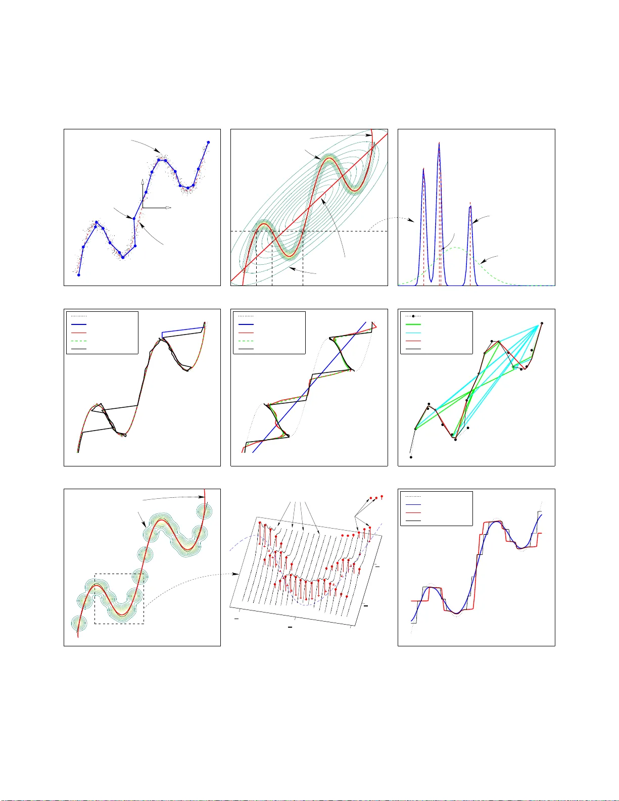
Reconstruction of sequen tial data with densit y mo dels ∗ Miguel ´ A. Carreira-P erpi ˜ n´ an Dept. of Computer Science, Unive rsity of T oron to 6 King’s College Road. T oron to, ON M5S 3H5, Canada Email: miguel@c s.toronto.edu Abstract W e introduce the problem of reconstructin g a sequence of multidimensional real vectors where some of the data are missing. T h is problem con tains regre ssion and mapping inv ersion as particular cases w h ere the pattern of missing data is indep endent o f th e sequence index. The problem is hard b ecause it inv olves possibly multiv alued mappings at eac h vector i n the sequence, where th e missing v ariables can take more than one v alue given the present v ariables; and the set of missing v ariables can v ary f rom one vector to the next. T o solv e this problem, we propose an algorithm based on t wo redundancy assumptions: v ector redun dancy (the data li ve in a low-dimensional manifold), so that the p resen t v ariables constrain the missing ones; and sequence redundancy (e.g. continuit y), so that consecutive v ectors constrain eac h other. W e capture t he lo w-dimensional nature of the data in a probabilistic wa y with a joint density mo del, here the generative top ographic mapping, whic h results in a Gaussian mixture. Candidate reconstructions at eac h vector are obtained as all the modes of the conditional distribution of missing v ariables given present v ariables. The reconstructed sequence is obtained b y minimising a global constrain t , here the sequence length, by dyn amic programming. W e presen t exp erimen tal results for a toy problem and for inverse kinematics of a rob ot arm. Keywords: missing data reconstruction, multiv alued (one-to-many) mappings, mapping inv ersion, Gaussian mixture mo des, constraint minimisation, dyn amic p rogrammi n g. 1 In tro duction W e co nsider the problem of re c onstructing a seq ue nc e of multidimensional rea l v ec tors where some comp onents of some v ecto rs are missing. As an example, consider a sp eec h utterance that is corr upted by another sound signal: at a given instant so me s peech sp ectral bands ar e corr upted by the other signal and ca n b e considered missing. A given sp ectral band may be missing at so me instan ts and present at other instants. The recons truction problem here is to obtain the v alue of the mis s ing sp ectral ba nds given the pre sen t ones, for the whole utterance. In the particular case when the co mponents or v aria bles that are missing are the same for all vectors o f the seq uence, the reco nstruction problem b ecomes a re g ression or mapping approximation (of the missing v a riables given the present o nes, or the Ys given the Xs). Regressio n methods (e.g. a neural net) usually estimate univ alued mappings (one-to-one or ma n y-to- one), where a given v alue of the prese n t v a riables results in a unique v alue for the missing v aria bles. This works well when there is an underlying function (in its mathema tical sense) that uniquely determines the miss ing v aria bles given the present o nes; but this is not the c ase generally , as for in verse mappings (r esulting from in verting a forward, univ alued map). F or exa mple, the p osition of the end-effecto r of a robo t arm is uniquely determined by the ang les at its joints, but not v ice versa (in verse kinematics). When the missing da ta pattern v aries alo ng the sequence, univ alued mappings will oc cur intert wined with multiv alued ma ppings (one- to-many). W e depa rt from the traditional p oint of view and define multiv alued mappings as the bas is o f our reconstructio n metho d: in one particular vector of the sequence, there may b e mo re than one v a lue for its missing co mponents that is c o mpatible with the v a lue of its pre sen t co mponents. A flexible way o f generating such mult iv alued mappings (of a n arbitrary subset o f v ar iables ont o another s ubset) is via co nditional distributions of a joint density model. Ho wev er , some of these v alues will not be compatible with the rest of the sequence, conside r ed globa lly: for ex a mple, they may res ult in physically impo ssible discontin uities of the inverse kinematics of the rob ot arm. T o break the ambiguit y of which reconstructed v alue to cho ose at each vector, we ass ume some prior informatio n is av aila ble that constr ains the sequence, in particular its contin uity: one must cho ose the reconstr ucted v alues such that the re s ulting sequence ∗ This pap er wa s written on Jan uary 27th, 2004 and has not b een up dated since then. 1 Examples of problem Exp erimental conditio ns z Observed v aria bles t T ra jectory of a mobile p oin t time, 1D spatial co ordinates, 3D Spo k en utterance time, 1D sp eec h feature vector, ≈ 1 3D Wind field on the o cea n surface spatial co ordinates, 2D wind velocity v ector , 2D Colour image spatial co ordinates, 2D R GB level, 3D T able 1: E xperimental conditions z and obse r v ed v ariables t for several examples of problems. is as contin uous as p ossible. Th us, we a ssume that the data have tw o kinds of r edundancy: (1 ) the vectors lie in a low-dimensional manifold and so knowledge of some vector co mponents constra ins the remaining ones (p oin twise redundancy); and (2) consec utive vectors lie nea r each other (acros s-the-sequence r edundancy). The rest of the pap er is o rganised as follows. Section 2 defines the data reconstruction problem. Section 3 explains how we der ive multiv alued functiona l relationships from conditional distributions. Section 4 e xplains how to use prior infor mation to co nstrain the multiv alued mapping s thus derived, and how to find the o ptimal reconstructio n. Section 5 s ummarises the re construction metho d. Sections 6–7 give exp erimental res ults. The remaining sections discuss the metho d, review related work and c o nclude the pap er. A preliminary version o f this work app eared as a conference publicatio n (Carreira -Perpi˜ n´ an, 2 0 00b). 2 Definition of the problem of data reconstruction Generally , w e define the pro blem of data reco nstruction as follows: given a data set { t n } N n =1 ⊂ R D wher e p art of the data ar e missing, r e c onstruct the whole data set to minimise an err or criterion . Let us exa mine in detail the elements of this definition. The data se t The data set must hav e some structure in or der that reconstr uction b e possible, i.e., there must be some dependencies b et ween the differ en t vectors in the set that give rise to redundancy . A t ypica l example is sequential data in which co nsecutiv e vectors are close to each o ther (o f course, not all sequences satisfy this). Such data can b e considered as the re sult of sampling in time a vector that is a contin uous function of the time. W e can generalise this notion as follows. Assume { t n } N n =1 are sa mples fr o m a contin uo us function F of an indep enden t v a riable z at po in ts { z n } N n =1 . W e call z the exp erimental c onditions ; z can b e the time (when the sample was taken), the p osition in space (where it w a s tak en), etc. Th us, t = F ( z ) is the sample point obtained at condition z . W e call t = ( t 1 , . . . , t D ) T the observe d variables . W e o bserve t but not nece s sarily z , a nd F is unknown. T able 1 gives so me examples. F g iv es to the co llection { t n } N n =1 the structur e or re dunda ncy that allows the reco nstruction of missing data. W e now have three dimensionalities: the dimensionality of the space T o f the t vectors that we obser v e, D ; the intrinsic dimensiona lit y o f the manifold M of T where the t vectors are co nstrained to live, L ; and the dimensionality of the v aria ble z , C , corres p onding to the batch of data { t n } N n =1 that we wan t to recons truct. These dimensionalities verify D ≥ L ≥ C . F or example (fig. 1), ima gine a n ant that w a lks o n the trunk of a tree ( L = 2) and take T as the Euclidean space ( D = 3) and z as the time ( C = 1 ); a giv en tra jectory of the ant will be 1D, but the r egion that the an t is allow ed to be on (the trunk) is 2D and in principle w e may find it anywhere in that 2D regio n (either by taking a very long tra jecto ry o r b y taking many different tr a jecto r ies). In the r est o f this pap er we a s sume D > 1. The case D = 1 do es no t allow to lo ok a t the relations hip b etw een v a riables, since there is only o ne ( t = t 1 ), and there fo re we cannot ma k e us e of the redundancy derived fro m a low-dimensional repr esen ta tio n. W e will also ass ume seque ntial data unless other wise noted, i.e., z is the time (or some other 1 D v ar iable), althoug h the treatment can b e generalised to any dimensionality C . W e will write { t ( n ) } N n =1 to denote a sequential data set, where n indicates a temp oral order in the da ta, re s erving the notation { t n } N n =1 for data sets which need not hav e any se q uen tial or der (in which case n is just a lab el). The pattern of missi ng data That p art of the data ar e missing mea ns that some of the N D v ariables { t nd } N ,D n,d =1 hav e missing v alues. W e say that the v alue of a given scala r v a riable t nd is pr esent if such v a lue was measured; otherwise, we say it is missing . Abusing the la ng uage, we will a lso sp eak of pres en t (miss ing) v aria bles to mean v ar iables whos e v alues are pres e nt (missing). The rea s ons for a v a lue to b e missing ar e multiple: the v a lue may not hav e b een measured; the v alue was measured but may hav e g ot lost, era sed or co rrupted; and so on, depe nding on the pa rticular problem. 2 P S f r a g r e p la c e m e n t s T (dimension D = 3 ) M (dimension L = 2) F ( z ) (dimension C = 1 ) t n Figure 1 : Dimensionalities involv ed in da ta reconstruction. The data, mea sured in a D -dimensio nal space T , liv e in a n L -dimens io nal manifold M . A particular da ta set { F ( z ) } of M has a dimens io nalit y C equal to that of the exp erimen ta l c o nditions z . The dimensionalities v e r ify D ≥ L ≥ C . -0.22 -0.07 0.28 -0.08 -0.06 0.24 -0.03 -0.27 0.18 -0.20 -0.00 -0.23 -0.44 0.08 -0.04 0.37 -0.29 -0.06 0.49 0.26 0.07 -0.48 0.14 0.43 0.08 0.03 0.29 0.27 -0.18 0.18 -0.08 0.14 -0.44 0.47 0.46 -0.29 0.02 -0. 29 0.10 0.49 0.23 0.34 -0.17 -0.12 -0.45 0.29 -0.09 0.13 -0.17 -0.22 -0.03 -0.44 -0.08 -0. 29 0.49 0.08 0.02 -0.07 -0.27 0.08 0.26 0.03 0.14 -0.12 -0.45 0.10 -0.44 0.29 0.07 -0.04 0.18 0.28 -0.08 -0.20 0.37 -0.48 0.27 0.47 0.49 0.29 -0.09 0.23 0.46 -0.18 0.14 -0.29 -0.00 -0.06 0.24 -0.23 -0.06 0.43 0.18 -0.29 0.34 0.13 P S f r a g r e p la c e m e n t s t 1 t 2 t 3 t 4 · · · t D t (1) t (2) t (3) t (4) t (5) t (6) · · · t ( N ) Original seq ue nc e Missing data pattern (mask) Observed seq uence Observed v ariab les V ec tors Present v alu e Missing v alue Figure 2: Schematic representation of the miss ing data. The black and white cells in the missing data pattern indicate missing and pres e nt v alues, re spectively . When the v a lues are corrupted in v ario us amounts rather than just b eing either missing or present , one could consider further ca tegories of uncer ta in ty in a v alue. This can be a b eneficial stra tegy for, e.g., rec o gnition of o ccluded sp eech (Co oke et al., 20 01). Ho wever, for the purp oses o f data r econstruction, it is not clea r what one should do with a v a lue that is neither prese nt (which m ust no t b e mo dified) nor missing (which must b e filled in). Therefore we will stick to the present/missing dic ho tom y . W e will also assume that ea c h v alue ha s b een classified as either present or missing, even though in some applications this task may not b e trivial. W e can repres en t the pa ttern of missing data a sso c iated with the data set { t n } N n =1 with a matrix (or mask ) M = ( m nd ) of N × D such that m nd = 1 if the v alue of t nd is present a nd m nd = 0 o therwise. The matrix M acts then as a mu ltiplica tiv e mask on the c omplete data set, i.e., the data set where a ll v alues a re present, as represented in figure 2 . W e obtain the pro blem of regre s sion (or ma pping approximation) in the particular case where m nd is indep enden t of n (in which case the mask o f fig. 2 has a co lumnar structure). W e will use the term r e gr ession-typ e missing data p attern if the patter n of missing da ta is constant ov er the s equence and gener al missing data p attern if it v aries. W e w ill use the term c omplete data set to mea n the data se t as if no v alues were missing and r e c onstru ct e d data set to mea n the data set w he r e the missing v a lues have b een filled in by a reconstructio n algo rithm. The algorithm describ ed in this pap e r is a pplica ble to any pattern of miss ing da ta, irre s pectively of why or how that pa ttern came ab out. Ho wever, if the missing data a re not mis sing completely at random (i.e., the patter n of missing da ta dep ends on the actual data; Little and Rubin, 1 9 87), then an y information a bout the mec hanis m of 3 missing data should b e taken in to account if p ossible, since it may further constra in the v a lues that the mis s ing v a riables ma y take. Reconstruction of the who le data set T o r e c onstru ct the whole data s et means to find a single estimate of each missing v alue. Generally , w e define four types of r econstruction a ccording to the co m binations o f the following character istics: • The num b er of ca ndidate reconstr uctions of a given entit y that ar e provided: single o r multiple r econstruc- tion. • The entit y that is b eing reco nstructed: p ointwise (or lo c al) for rec onstruction o f a vector t ( n ) given infor- mation pres en t in t ( n ) only , and glob al for reconstr uction o f the whole sequence or data set { t ( n ) } N n =1 given information present in it. Using this terminology , we seek a single global reconstruction of the data set. A method that provides single p oin t- wise reconstruction can only provide s ing le globa l reconstr uction; s tandard r e gression a nd mapping approximation are examples of such metho ds. But single global r econstruction ca n b e a ttained by a n appropr iate combination of a collection of multiple point wise reconstr uctions; the metho d pro pose d in this pa per do es this. Error criterion In this pap e r we use the square difference betw een the true and the reconstruc ted v ector s (av erag ed ov er the sequence) as a meas ur e of the reconstruction erro r. Other criteria ar e a lso p ossible. Notation W e use the following notatio n to select co mp onents (v ar iables) of a vector. If t = ( t 1 , . . . , t D ) T ∈ T is a D -dimensional rea l vector and P ⊂ { 1 , . . . , D } is a set of indices, then t P represents the v e ctor c o mposed of those c o mponents of t whos e indices are in P . F or example, if P = { 1 , 7 , 3 } and M = { 2 , 5 } then p ( t M | t P ) is p ( t 2 , t 5 | t 1 , t 3 , t 7 ). This notation is c o n venien t to repr esen t arbitrary patter ns of missing da ta, where the pr esen t or missing v ariable s a t po in t n a re indicated b y sets P n and M n satisfying P n ∩ M n = ∅ and P n ∪ M n = { 1 , . . . , D } . Abusing the no tation, we may sometimes write t n, P or t ( n ) P to mea n t n, P n or t ( n ) P ( n ) , resp ectively . O ften, we will also use x and y to refer to the present a nd missing v aria bles, respe ctiv ely . 3 Deriving m ultiv alued functional relationships from conditional dis- tributions An y kind of reco nstruction is based o n a functional relatio nship of what is missing given what is pres en t. This section discusses tw o central ide a s. T he first one is that o ne can define a functiona l r elationship x → y ( y a s a function o f x ) from the conditional distribution o f y given x b y picking representativ e p oints of this distr ibution. The seco nd one is that underlying a m ultimo dal conditional distribution there (often) is a m ultiv alued functional relationship a nd that it is wrong to summarise such a distr ibution with its exp ected v a lue. Instead, we prop ose the use of a ll the mo des of a co nditional distribution to define a multiv a lued functional relations hip and thus to define mult iple p o in twise rec o nstruction. W e assume that the conditiona l distribution comes from a probability density function (p df ) p ( t ) for a ll the observed v aria bles t = ( t 1 , . . . , t D ) T . In gener al, we use the terms pr e dictive distribution for a distribution co n taining informa tion ab out the missing v a riables (p erhaps different from the conditiona l) and c andidate (p ointwise) r e c onstr u ctions for the v alues used to fill in the missing v aria bles (perhaps differe nt from the mo des). 3.1 Informativ e, or sparse, distributions A conditional distribution p ( y | x ) which consists of s e v er a l s harp pe aks conv eys informatio n ab out a functional relationship in that the pr obabilit y mass is c oncen tr a ted a round a few po in ts. W e can construct a mult iv alued mapping x → y by picking sev e r al particularly informative points of the domain of p ( y | x ) (see fig. 3). In gener al, we say that a D - dimensional pdf p ( t ) (p ossibly the distribution of t conditioned on the v alues of some other v a riables) is informative or sp arse if the probability mass is c oncen tr a ted around a low-dimensional manifold. Con versely , if the probability mas s is spr ead ov er a D -dimens io nal regio n then we say that the p df is uninformative . W e th us state the principle that highly informa t ive distribut ions c an b e assimilate d t o (p ossibly multivalue d) functional r elationships . As we de fine it, the concept of dis tribution spars eness is a proba bilistic extension of the concept of low- dimensional manifold. Thus, a D -dimensiona l pdf defined around a p oint / curve/surface is spar se for D ≥ 1 / 2 / 3, 4 P S f r a g r e p la c e m e n t s y y x y 0 y 0 y 1 y 1 y 2 y 2 x 0 p ( y | x = x 0 ) p ( x, y ) Figure 3: A conditional distribution can imply a m ultiv alued functional r elationship. L eft : jo in t probability density p ( x, y ), represented by the shaded area; the black dots show a sample typical from that density and the thick line indica tes a low-dimensional manifold. Ri ght : mult iv alued mapping x → y from the m ultimo dal conditional distribution p ( y | x ). F or x = x 0 we obtain y 0 , y 1 and y 2 as poss ible v alue s for y . resp ectively , a nd so on. Our definition of spar seness is v ague, since the term “concentrated around” is rela tiv e— just how m uch pro babilit y mass a nd how near the low-dimensional manifold? F or the purp ose o f deriving func- tional relationships fro m c o nditional distributions this definition suffices. Carreir a-Perpi˜ n´ a n (20 01) disc usses the issue of measur ing spar seness quan titatively . A conditional distribution p ( y | x ) ma y b e informative for so me v alues of x and uninformative for o ther v alues of x . If we requir e that p ( y | x ) b e informative for any v alue of x , then the joint density p ( x, y ) must be itse lf an informative distribution, since p ( y | x ) ∝ p ( x, y ). 3.2 Unimo dal distributions: L 2 -optimalit y of the mean F or unimo dal distributions, it makes sense to summa r ise the dis tribution with a single p oint. Whic h p oint to choose dep ends on what erro r criter ion we wan t to minimise. If w e pick the p oint that minimises the a verage dis - tance (with resp ect to the distribution of t ) to ev er y other point in the domain of t , ˆ t = arg min ˆ t ∈T R T p ( t ) d ( t , ˆ t ) d t , then the optimal p oint is the mean of p ( t ) if d is given by the L 2 -norm (Bishop, 1995, pp. 201–2 05) and the median if d is given by the L 1 -norm (DeGro ot, 1 986, p. 209–210 ). F o r s ymmetric distributions the mean, median and mo de coincide, but for skew ed distributions they differ . Howev er, the median do es not hav e a natural gen- eralisatio n to more than 1D. A nu mber o f a pproaches exist that derive univ alued ma ppings fro m the conditional distribution, usually via the mean (see section 9.2 ). 3.3 Multimo dal distributions: the mean considered harmful The mean of a multimodal distribution can lie on an area of low pr o babilit y , th us being a highly unlikely r ep- resentativ e o f the distributio n. W orse s till, it may lie outside of the supp ort of the r andom v ariable when such suppo rt is not a conv ex s et, since the mea n is a conv ex sum itself (and this can ha ppen even if the distribution is unimo dal); this fact has b een po in ted out in the co n text of in verse pr oblems (Jorda n, 1990 ; J ordan and Rumel- hart, 19 92). In spite of this, the mean re mains the most co mmo n choice of representativ e p oin t of a multimodal distribution, p ossibly due to b eing o ptimal with resp ect to the L 2 -norm (as lo ng as one is cons trained to choose a single p oin t) a nd to its ease of calculation. A b etter choice a re the mo des. Unlike the mea n, any mo de by definition must lie inside the supp ort of the random v ar ia ble and have a lo cally high pr obabilit y density . In gene r al, calculating the mo des of a multiv ar iate distribution is difficult b ecause one do es not know how many mo de s there are a nd b ecause computing each one of them cannot b e done analy tically . How ever, for Gauss ian mixtures, Carreir a-Perpi˜ n´ a n (200 0a) gives algor ithms for finding all the mo des 1 . The algorithms can a lso compute er ror bars for each mo de, thus estimating lo cally the erro r , though this will not be used here . 1 The algorithms wo r k by starting a hill-climbing search f rom ev ery centroid. A Gaussian mixture in 2 or more dimensions can ha ve more mo des than components even if all the components ha ve the same, i s otropic co v ariance (Carrei r a-P erpi ˜ n´ an and Williams, 2003b,a), so the algorithms can miss some mo des. How eve r , this situation is very i nfrequen t. 5 But then how do es one deal with a multiv alued choice? In the absence of additional information, all we can do is to keep a ll the mo des, since any of them is a likely representativ e of the distribution. This implies defining a m ultiv alued functional relatio nship. Thus, w e pro pose to selec t al l the mo des of the c onditional distribution a s representative po in ts of it. 3.4 Sampling the predictiv e distribution Another metho d to pick representativ e p oints o f a distributio n is to sample from it. This mak es sense when there are few pres en t v a riables, s o that the missing v ariables ar e so under determined that they can take v a lues o n a contin uous manifold: in this case, the mo des of a co nditio na l distr ibution are effectively a pa rticular sample from that manifold. Computationally , sampling can also b e more attra ctiv e than finding all the mo des. How ever, when the missing v ar iables are constrained to take a finite num ber of v alues, this do es not make m uch sense. Unless the conditiona l distributio n is very sharply p eaked around its mo des, sampling will return v a lues that by definition ar e corr upted by noise: sometimes they may fall in areas far from the main proba bility mass b o dy or igno re low-probability bumps (which may repr esen t infrequent but le g itimate reco nstructions). A further, ser ious pro blem is how to set the n umber of sa mples to obta in, whic h will certainly lo cally under estimate or o verestimate the true n umber of v a lues that the missing v aria bles can take. Missing a cor rect p oint wise reconstructio n or genera ting a wrong one may a ffect the g lobal rec o nstruction, not just the lo cal one, via the contin uity co ns train t (see sectio n 4). Our expe r imen ts show tha t the sampling strategy p erfor ms consistently worse than bo th the mean- and mo de-based approaches. 3.5 Join t densit y mo del of t he observed v ariables F or a generic missing data pa ttern we need to be a ble to obtain the conditional distribution for any co m bination of missing and prese n t v ariables , which r equires estima ting a joint density mo del o f all the obs erved v aria bles. The join t density em b o dies the relation of an y subse t o f v ar iables with any other subset of v ar iables; a ll w e need is to compute the a ppropriate conditional distribution, which in turn requires a marginalisa tion: p ( t M | t P ) = p ( t M , t P ) /p ( t P ) = p ( t ) /p ( t P ). Therefor e, we are free to cho ose the metho d b y which we estimate the join t density a s long as the estimato r allows easy ma rginalisation. The density mo del should b e estimated offline using a training set different from the one that is to b e reconstruc ted. T ypica lly , the training set will hav e no missing data, althoug h even if it do es, it is p ossible to tr ain the mo del using an EM algorithm (e.g. Ghahramani and Jordan, 1994 ; McLachlan and Krishnan, 1997). A suitable cla ss of density mo dels are cont inuous latent v aria ble models , since the point wis e redundancy implies an int r insic low dimensionality of the o bserved v a riables (Carr eira-Perpi˜ n´ an, 2001). The distribution of the obse r v ed v aria bles is sparse in the sense of section 3 .1. The densit y model m ust be able to represent m ultimo dal densities. This disca rds linear-no rmal mo dels (facto r analysis and principal comp onent a nalysis). It s ho uld also allow an eas y computation o f conditio na l distributions. Useful models include the g enerative topog raphic mapping (GTM; Bishop, Sv ens´ en, and Williams, 199 8b), mixture s of factor analy sers (Ghahr amani and Hin ton, 1 996) a nd mixtures of principal co mponent a nalysers (Tipping and Bisho p, 1 999). F o r all these mo dels the dens it y of the observed v aria bles has the form o f a (constra ine d) Gaussian mixture a nd the num b er of tunable par a meters can be kept reasonably lo w while keeping the ability to represent a broa d class o f m ultimo dal densities. W e can also directly use Gaussian mixtures or (nonparametr ic) kernel density estimation, b oth of whic h hav e the pr oper t y of universal density a pproximation (Titterington et a l., 1985; Sco tt, 199 2 ). In this paper we use the GTM; w e refer the reader to the o riginal paper s (Bishop et al., 1998b,a ) for details on this mo del. Hereafter we will assume tha t the joint density has the form of a Gaus sian mixture, whose par a meters were estimated from a data sample in an unsup ervise d w ay . Computing conditiona l distributions is then s tr aight fo rw a rd (for a dia gonal Gaussian mixture, this re quires little more than crossing o ut rows a nd columns). Finding a ll the mo des can b e done with the a lgorithms of Car reira-Perpi ˜ n´ an (2000a). In the particular cas e wher e the pattern of missing data is co ns tan t, one can just mo del the appropriate conditional distributio n rather than the joint density , of course (section 9.4 ). 4 Use of pr ior information to constrain m ultiv alued mappings So far w e hav e exploited the r e dundancy b etw een comp onen t v aria bles of a given data point (via the co nditional distribution) to constrain the p ossible v alues of the missing v aria bles, but this can still result in m ultiv alued mappings, as w e hav e seen. In the absence of any a dditional information, the answer to the reconstruction 6 problem would b e those multiv alued mappings. W e now turn to the cas e of using extra information ab out the problem to constr ain the p ossible v alues so that we o btain a unique global reconstruction of a data set. 4.1 Con tinu ity constrain ts F or many practical case s, additional informatio n comes from the redunda nc y b e t ween data p oin ts and dep ends on the exper imen tal conditions. The most usual suc h co ns train t is g iven b y c ont inuity of the v ar iables as a function of the exp erimental co nditio ns, t = F ( z ): nearby v alues of z pro duce nearby v alues of t , or “ d ( t n , t n +1 ) is sma ll” according to a dista nce dep enden t o n the problem. In this c a se, t ypica lly z is a physical v ariable such as the time (or spac e) and then t is a measured vector that dep ends contin uo us ly on it, resulting in a contin uous tra jectory (or field). In genera l, we can define co nstraints on the tra jector y b y b ounding via a nor m the deriv atives of the function F (if they exist), num e r ically approximating each der iv ative by a finite-difference scheme in terms o f the av a ilable measur e s a t z 1 , z 2 , . . . , z N and applying suitable bo undary conditions at the tra jectory ends (e.g. to consider op en o r closed tra jectories). Continuity (whic h pe na lises sharp jumps) results fro m the first de r iv ative, while smo othness (whic h pena lis es s ha rp turns) res ults from the se cond. This results in the norm o f a linear combination o f p oints near t n . Actual examples are given in section 4.3. The nor m depends o n the problem, but t y pically will b e the Euclidean or sq uared Euclidean norm. If different v a riables hav e different units or sca les it may be co nvenien t to use a weighted norm. The squa r ed Euclidean norm has the computationa l a dv antage that it sepa rates additively along ea c h v ar ia ble a nd so for a consta n t missing data pattern ( M n = M ∀ n ) we need only conside r the missing v ariables (since the present ones contribute a constant additiv e term). It als o results in constra in ts that a re quadratic forms on the v ariables { t nd } N ,D n,d =1 , though this makes no difference in the constr ain t minimisation. Another t yp e of co nstraint that has often b een found useful in in verse problems is a qu adr atic constraint ( t n − t 0 ) T Q ( t n − t 0 ), which ca n b e int er preted physically as a n energ y in mechanical systems. In particular , k t n − t 0 k 2 corres p onds to the p oten tial energy of a harmonic osc illa tor with re sting po sition at t = t 0 and restoring constant k = 2 . 4.2 Constrain t by forwa rd mapping In the particular ca se where the rec onstruction problem is a mapping inv ersion problem, we can us e the k no wn forward (direct) mapping as a further co nstraint . The forward mapping g maps the missing v a riables onto the present o nes: t P = g ( t M ), where P and M ar e indep endent of n (i.e., the s ame for all data p oin ts). Thus, given the v alues of t P and given a candidate r econstruction ˆ t M (for example ˆ t M could b e o ne o f the mo des of p ( t M | t P )), then the distance b et ween ( t P ˆ t M ) and ( g ( ˆ t M ) ˆ t M ) should b e as small as p ossible. In the ide a l case wher e the pro cedure that provides candidate reconstructions (in this pa per, the modes of the conditional distribution) was p erfect, this constraint would have no effect, since every ˆ t M would exactly map onto t P . In reality , cor rect reconstructions will give small, but nonz e ro, differ ences b et ween t P and g ( ˆ t M ), while incorre ct reconstr uctions (such as spurio us mo des) will g enerally give a muc h la rger difference. Thus, the constraint by forward mapping ca n help to discard such incor rect reconstructions. 4.3 Minimisation of a global constrain t The co nstraint s intro duced ab ov e are by definition lo cal and gener ally take the form of the (sq uared) norm o f a linear combination of neighbo uring p oin ts; e.g. k t n +1 − t n k . No w we der iv e from such lo cal constr ain ts a glob al c onstr aint that in volves the whole da ta set. This wa y we define an ob jectiv e function dep ending on a ll missing v a riables a nd then find the c o m bination of candidate p oint wise r e constructions that minimises it. W e will then hav e a single g lobal recons tr uction tha t should b e a go o d approximation to the complete data set. The role o f the glo bal constraint in breaking the nonuniqueness o f the reconstruction is analogo us to that o f regularis ing op erators for ill-p osed problems (Tikhonov a nd Arsenin, 1977). 7 P S f r a g r e p l a c e m e n t s B E n = 1 2 3 4 · · · N ν n = 5 2 4 1 · · · ν N Q N n =1 ν n p ossible paths          Candidates to reconstruct t ( n ) Figure 4: Constraint minimisation as a shortes t path pr o blem in a lay ered graph. There a re ν n no des in lay er n in the graph, whic h are the candidate p oint wise reconstructio ns of t ( n ) M ( n ) (the modes of the conditional distribution t ( n ) M ( n ) | t ( n ) P ( n ) ). There are N lay ers and a single glo bal reco nstruction of the data set defines a left-right (or right-left) path passing through all layers exactly onc e (one such path is highlighted). By imagining fictitious end no de s B and E fully connected by z e ro-cost links to the end lay ers 1 and N , resp ectiv e ly , we can r eformulate the pro ble m as that of finding the shortest path b etw een B and E . Each edge in the gr aph is undirected a nd has an a sso ciated cost given by the contin uity cons train t (the distanc e b etw een the r econstructed points). W e can define a g lobal co nstraint b y adding the loca l co ns train ts for each point in the seq uence, th us obtaining: Contin uity , C def = N − 1 X n =1    t ( n ) − t ( n +1)    (1) Smo othness, S def = N − 1 X n =2    t ( n +1) − 2 t ( n ) + t ( n − 1)    (2) Quadratic, Q def = N X n =1 ( t ( n ) − t 0 ) T Q ( t ( n ) − t 0 ) (3) F or w ar d-mapping, F def = N X n =1      t ( n ) P t ( n ) M  −  g ( t ( n ) M ) t ( n ) M      . (4) In eqs. (1)–(2) we have used first- and s econd-order forward differences in C a nd S , resp ectively , a ssuming that the exper imen tal condition v aria ble z is sa mpled regularly; if this is not the c a se, then one should w eight term n by 1 / ( z n +1 − z n ). Note that C is the length of the p olygo nal tra jectory pa ssing thro ugh t (1) , . . . , t ( N ) . W e can define a globa l co nstraint as a linea r co m bination of constr ain ts such as those ab ov e, but in this pap er we will concentrate in C . The global constraint is a function of the miss ing v aria ble s { t ( n ) M ( n ) } N n =1 . Thu s we arrive at the following minimisation pro blem: Reconstruct the data set as arg min { t ( n ) M ( n ) } N n =1 ∈S C  { t ( n ) M ( n ) } N n =1    { t ( n ) P ( n ) } N n =1  where the search space S is the Cartesia n pro duct of the N sets of candidate reconstructio ns for each t ( n ) M ( n ) (i.e., each set co n tains the mo des o f p ( t ( n ) M ( n ) | t ( n ) P ( n ) )). This is a combinatorial optimisatio n pro blem that ca n b e expressed as finding the shortest pa th in a layered g raph, as r epresented in figure 4 . Ca lling ν n ≥ 1 the num b er of candidate po in twise r econstructions at point n , the total num b er of pa ths is Q N n =1 ν n , which in an average case is of exp onential o rder in N . F ortunately , ther e are efficient alg orithms b oth for global (exact) and lo cal (approximate) minimisation. 4.4 Global minimisation: dynamic programming The problem of finding the shortest path in a layered graph is a particula r ca se o f that of finding the shortest path in an acyclic g raph and can b e conv eniently s o lv ed by dynamic pro gramming (Bellman, 1957; Bertse k as , 1987). W e can apply dynamic progra mming because for this pr o blem the following principle of optimality for a decision policy ho lds: r e gar d less of the p olicy adopte d at pr evious stages, the r emaining de cisions must c onst itute an optimal p olicy , where here a stage is a layer in the gr aph a nd a p olicy is a s equence of decisions (i.e., a sequenc e 8 initiali s e for i = 1 , . . . , ν 1 F or each no de of lay er 1 A 1 ,i ← [ a 1 ,i ] Singleton path l 1 ,i ← 0 P a th length end for n = 2 , . . . , N F or each lay er for i = 1 , . . . , ν n F or each no de of lay er n j ∗ ← arg min j =1 ,...,ν n − 1 {k a n − 1 ,j − a n,i k + l n − 1 ,j } Choos e optimal link A n,i ← [ A n − 1 ,j ∗ ; [ a n,i ]] Short est pa th to nod e i l n,i ← k a n − 1 ,j ∗ − a n,i k + l n − 1 ,j ∗ P a th length end end i ∗ ← arg min i =1 ,...,ν N l N ,i return A N ,i ∗ Short est pa th Figure 5: Dynamic pr ogramming a lgorithm for global c o nstraint minimisation. Sequences of no des are written in square bracket s and [ A ; B ] means the concatenation of sequences A and B . of chosen no des). This lea ds us to a n alg orithm where the dec is ion of what link to cho o se is taken lo cally (at ea ch lay er n ), but ν n paths must b e kept. Figure 5 gives the forward recur sion version of the dynamic pro gramming algorithm (sta rting from lay er 1) for a glo bal contin uity c onstraint C . Due to the symmetry of the problem, a backw ard algor ithm (starting fro m layer N ) is equiv a len t. The algo rithm req uires the following definitions: { a n,i } ν n i =1 The set of candidate point wise reconstructions for t ( n ) ; thus a n,i is no de i of layer n in the graph. A n,i Minimal length path from lay er 1 to no de i o f layer n , for i = 1 , . . . , ν n . Thus, A n,i = [ a 1 , • ; a 2 , • ; . . . ; a n,i ] where • indicates some no de. l n,i T o tal leng th of A n,i , i.e., l n,i def = P n − 1 m =1 kA n,i ( m ) − A n,i ( m + 1) k , where A n,i ( m ) is the m th element of the s equence A n,i . W e dis regard the unlikely ca se of ties, where the arg min j =1 ,...,ν n − 1 op eration may r eturn sev er al v alues of j . The dynamic pro gramming algorithm examines each link in the graph (i.e., each pair of no des in adjacent lay ers) only once, thus ac hiev ing its miss io n v ery efficiently . 4.5 Lo cal minimisation: greedy algorithm A more intuitiv e and slightly faster algorithm is obtained as a greedy version o f dynamic progra mming : at lay er n , it simply selects the minimal co st edge (i.e., the closes t no de). The star ting p oint can b e any no de in any lay er n 0 , but to improve the chances of getting a goo d path, it is b etter to s ta rt in a lay er ha ving very few nodes (hop e fully just one). The a lgorithm greedily pr ocee ds from n 0 left wards to 1 and r ig h tw ar ds to N , since all edges are undirected. Unlik e dynamic prog r amming, this algor ithm needs only keep a single path a t any time r ather than ν n paths, but it do es not nece s sarily find a path of g lo bally minimal cost. Our exp eriments show that it usually leads to p o o r solutions, not just in terms of a high v alue of the constraint, but also as yielding a high reconstructio n err or o f the dataset—which is our ultimate c r iterion. Such solutions are s e nsitiv e to the choice of starting lay er n 0 . Also, the g reedy algo rithm has a tendency to obtain reconstr uc ted tra jectories that r etrace themselves a t tur ning p oin ts a nd hav e abrupt jumps. 5 Summary of the metho d W e can now summar ise o ur r econstruction metho d (see also fig. 9). The fir st step is done offline and inv olves estimating a Gaussia n-mixture join t density model p ( t ) of the observed v ariables, using a complete dataset { t n } N ′ n =1 (w e us e GTM in this pap er). At reconstr uction time, we are given a sequence { t ( n ) } N n =1 with missing data. Then: 1. F or ea c h vector t ( n ) in the sequence, n = 1 , . . . , N : 9 • Compute the conditional distribution p ( t ( n ) M ( n ) | t ( n ) P ( n ) ) of the missing v ar iables given the prese nt ones. This is a Gaussia n mixture to o. • Find all the mo des of this conditional distributio n. These ar e the ca ndidate reconstructio ns for t ( n ) . 2. Minimise the tr a jector y length C  { t ( n ) } N n =1  ov er the set of candidate reconstr uctions using dynamic pro- gramming to yield the reco nstructed s e quence. 6 Exp erimen ts: 2D to y example In this section we study the p erformance of the r econstruction metho d with a 2D toy problem with observed v a riables  t 1 t 2  . The mapping t 1 → t 2 is many-to-one and so easy to estimate b y tr aditional metho ds, but the mapping t 2 → t 1 is one-to-many , as is the mapping ∅ →  t 1 t 2  . W e co nsider the forward, nonlinea r mapping g ( x ) def = x + 3 sin x for x ∈ [ − 2 π , 2 π ], which r esults in 1D data ( L = 1) obs erved in D = 2 dimensions by ta king t =  t 1 t 2  with t 1 = x and t 2 = g ( x ); see fig. 6A. The forward mapping g is injectiv e only in parts of the domain and so the inv e r se mapping g − 1 is sometimes multiv alued. The task is to r e c onstruct a (po ssibly no is y) sampled tra jectory of N 2D p oints such as tha t of fig. 6A with missing data. The reconstruction err or is c o mputed as the average squar ed erro r 1 N P N n =1   t ( n ) − ˆ t ( n )   2 , where { t ( n ) } N n =1 is the origina l, c o mplete tra jector y and { ˆ t ( n ) } N n =1 the tra jectory reconstructed by a par ticular method. Five types of N × 2 mas k are considered: • M fwd where t 2 is alwa ys missing (regre s sion t 1 → t 2 , 50% missing data); • M inv where t 1 is alwa ys missing (regre s sion t 2 → t 1 , 50% missing data); • M 75% , M 50% , M 25% where any of t 1 , t 2 are missing at random (75%, 5 0%, 2 5% miss ing data, respe ctiv ely). M fwd and M inv are regre s sion-type ma sks, while M 75% – M 25% are general missing data patterns. By applying the mask to a co mplete tr a jector y , w e obta in a tra jectory with missing data (see fig. 2). As training da ta for the joint densit y mo del p ( t ), we generated a s huffled (i.e., without seq ue ntial o rder) training set { t n } N ′ n =1 with N ′ = 1 00 0 p oints sampled from the curve with additive nor mal ( 0 , σ 2 I ) noise for σ = 0 . 2. W e used it to train 3 mo dels 2 (fig. 6B): • A factor analys er with one factor. W e use this as a linear- Gaussian density mo del baseline. • A m ultilay er p erceptro n (MLP) with a s ingle hidden lay er of 48 units, trained to minimise the squa red reconstructio n err or using s tochastic gradient descent and small, random starting v a lue s for the w eig h ts. W e us e this as univ er sal mapping approximator baseline. • A 1D GTM with a grid of K = 200 p oin ts and 9 Gaussian basis functions of width equal to the separ ation betw e en ba s is functions centres, all in the [ − 1 , 1] interv al (see Bishop et a l., 1 998b). This results in a Gaussian mixture with K = 200 c o mponents all with the same, isotropic cov ariance. W e us e this to implemen t mean- and mo de-based metho ds. W e c ompared the following re c onstruction methods ba sed on GTM: mean Sin g le point wise rec onstruction b y the conditional mean (section 3.2). gmode Single p oint wise reco nstruction by the glo ba l mo de of the conditiona l distribution. rmode Single p oint wise reco nstruction by a rando m mo de (all mo des are taken equally lik e ly). cmode Single p oint wise reco nstruction by the closest mo de , i.e., the mo de of the conditional distribution that is closest in Euclidean distance to the true v a lue of the orig inal s equence (of course, unknown in practice). The cmode gives a low er b ound o f the rec o nstruction error achiev able by a ny mo de-based metho d ( gm ode , rmod e , grmode , dpm ode ) a nd tells us how muc h usable recons truction information is contained in the conditional mo des. grmode Single p oin twise r econstruction b y the mo de of the c onditional distr ibution that is clo s est in Euclidea n distance to the previously r econstructed point, i.e., a greedy minimisation of C (section 4.5 ). 2 W e gr atefully ac knowledge the use of M atlab co de by Markus Svens ´ en (to train GTM) and Ian Nabney and Chr i stopher Bishop (Netlab, to trai n MLPs), b oth fr eely av ailable at http://www.ncrg. aston.ac.uk . 10 dpmode Multiple po in twise reconstruction b y the mo des of the conditiona l distribution follow ed by dynamic pro - gramming minimisation of C to se lect the global reconstructio n (section 4.4). The contin uity c onstraint C is based on the unw eighted E uclidean distance, eq. (1). This is the metho d we a dvo cate in section 5. meandp Like dpmode except that if the conditional distributio n is unimo dal, we use its mean r a ther than its mo de. This is intended to accoun t for skewed unimo dal conditional distributions. sampdp Multiple p oint wise re c onstruction by S = 6 sa mples o f the conditiona l distributio n (section 3.4 ) follow e d by dynamic progra mming minimisation of C to select the glo bal reconstruction. W e to ok S slightly larger than the maxima l num b er of inv er se branches o f g − 1 (equal to 3) so that all the branches hav e a c ha nce to contribute but without facilitating the app earance of outliers . Additionally , we co mpared with the metho ds fa for fa c to r analysis, for which the mean- and mo de-based metho ds coincide (b eing a symmetric, unimo dal de ns it y); and mlp for the mu ltilayer p erceptron (but only for masks M fwd and M inv , which co rresp ond to re g ression patterns of missing data). W e r an a num b er of exper imen ts o f whic h we discuss a repr esen ta tiv e selection (fig. 6, table 2). The s a me basic results were confirmed with many randomly generated training sets , mas ks and tra jectories to b e reconstr uc ted. Additional exp eriments are given in Carreira -Perpi˜ n´ an (20 01), including further mas ks (e.g. data missing by blo c ks ) and mo dels (e.g. full-cov ar iance Gauss ian mixtures, MLP ensembles). W e rep ort v arious a spects of the results next. Metho d com parison Based on these exp eriments we can draw the following c onclusions about the metho ds: • As exp ected, fa is alwa ys muc h worse than mean for any ma sk, since the fo r w a r d mapping is nonlinea r; and for b oth masks M fwd and M inv , mlp was practically equal to the mean . • Since our GTM mo del is very close to the tr ue density , the mean a pproximates ex tr emely well the forward mapping (mask M fwd , not shown in fig. 6), b eing univ alued. It fails with the inverse mapping (mask M inv , fig. 6E), this b eing mult iv alued: the univ alued mea n mapping tr a vels through the midp oin ts of the inv erse br anc hes , blending them into a sing le branch. Because of the s ymmetry o f the forward mapping, the midp oint of these bra nches alwa ys happ ens to coincide with one o f the branches a nd so the result is better than it should b e in a general cas e lacking symmetry (where the m ean will not b e a v alid in verse). The me an also fails for gener al masks (e.g. ma sk M 50% , fig. 6F), although, as pr e dic ted by the theor y , in terms of average reco nstruction error it is still the b est metho d ba sed o n single point wise reconstr uction (the others b eing gmod e a nd r mode ). Figure 6 (following page) : Recons tr uction results for the toy pro blem of section 6. This figure is b est viewed in colo ur . All panels (except C and H ) s ho w the rectangle ( t 1 , t 2 ) ∈ [ − 2 π , 2 π ] × [ − 2 π , 2 π ]. The panels ar e a s follows (see ma in text for details). A : the tra ining set for the dens it y mo dels (dots), the underlying data manifold (dashed line) a nd a sample no isy tra jectory (so lid circ le s). B : contour plots of the joint density mo dels: GTM (with K = 200 Gauss ia n comp onents) and F A. C : the co nditional distributions p ( t 1 | t 2 ) for a v alue t 2 = − 3 . 8 (horizontal dashed line in panel B ). F or GTM, this co nditional distribution contains 3 mo des (co rresp onding to the circles in B ) while for F A it is a broad Gaussian whose mean falls out of the data. D, E : recons tr uction of a noiseles s tra jector y with N = 100 p oints (original) b y several metho ds , for the mask M inv (i.e., for ea c h p oint in the tra jector y , t 2 is present and t 1 is missing). In D , the or iginal tra jectory is a lmost indistinguisha ble fro m dpmode and cm ode , while grm ode a nd sampdp pro duce reconstr ucted tra jector ies with retracings and shor tcuts. In E , the metho ds fail: fa returns a linear tra jector y , while gmode , mlp and m ean return a univ alued ma pping with discontin uous jumps b etw een branches (see the figure sidewa y s ). F : re c o nstruction of the noisy tra jector y of panel A with N = 20 p oints (origina l) by several metho ds, for the ma s k M 50% (i.e., for each po in t in the tra jector y , any of t 1 or t 2 is miss ing 50% of the times). cm ode and d pmode give very go o d re c o nstructions, w hile mean and gmode fail. The jumps to the po int in the cen tre ( mean ) a nd the top-rig h t cor ner ( gmo de ) o ccur whe n both t 1 and t 2 are missing a t one p oint of the tra jectory . G : GTM density mo del with only K = 20 Gaussian co mponents, resulting in a nonsmo oth dens it y . H : blowup of the box in panel G sho wing the conditional distributions p ( t 2 | t 1 ) at several v alues of t 1 (the red lines) a nd their mode s (the circles • ) a nd means (the crosses +). The dotted line is the da ta ma nifold. Note how where the Gaussian comp onents are widely separated, p ( t 2 | t 1 ) has mor e than one mo de even though t 1 → t 2 is univ a lued. I : re construction results for the no iseless tra jectory using the no nsmoo th GTM mo del of panel G , fo r several metho ds and mask M fwd (i.e., for each po int in the tr a jector y , t 1 is pr esen t and t 2 is missing). 11 P S f r a g r e p la c e m e n t s t 1 t 1 t 2 t 2 T r aining set Noisy tra jectory Mapping t 2 = g ( t 1 ) GTM density & latent ma nifold GTM density & latent ma nifold F A densit y & latent manifold mode mode mode mean cond. distr. p ( t 1 | t 2 ), GTM cond. distr. p ( t 1 | t 2 ), F A Mask M inv Mask M inv Mask M 50% Mask M fwd original original original original mean mean mean fa mlp gmode gmode grmode dpmode dpmode dpmode cmode cmode cmode sampdp Cond. distr. p ( t 2 | t 1 ) mo des − 2 π − 4 3 π − 2 3 π 0 2 3 π 4 3 π 2 π − 2 π − 4 3 π − 2 3 π 0 2 3 π 4 3 π 2 π A B C D E F G H I 12 • Both g mode and rmode result in discontin uous ma pping s, with frequent branch switches, but unlike the mean they a lw ays pr o v ide with v alid inv er ses, b ecause they track bra nc hes. gmo de gene r ally outp erforms rmode —the latter can be consider ed as the chance baseline for s ing le po in twise r econstruction by the mo des. • cmo de ac hieves pr actically zero reco nstruction erro r for a ll mas ks consider ed, v astly outp erforming the mean to o (except, marginally , sometimes with mask M fwd , where mean is optimal). This demonstrates that the mo des of a go od conditional dis tr ibution contain informa tio n that can p otentially achiev e near -zero reconstructio n err o r; the pro blem lie s in the sele c tio n of a go od cons tr ain t that discards the wro ng modes. • Much of the mo des’ informatio n is recovered by dpmode , which outp erforms or equals any other metho d, including me an , for any mask. Even for the forward mapping, where mea n is g ua ranteed to b e optimal o n the av e rage, dpm ode s till p erforms as well as the mean (it a c tually outp erforms it in table 2A, row M fwd , but this is an isolated instance). Its p erformance is degra ded only slightly for very high amount s of miss ing data (e.g. mask M 75% ), where the o ther metho ds incur huge errors. F or regress ion problems (masks M fwd and M inv ), dpmode may per form worse than m ean in t wo situations analysed b elow: nonsmo oth density mo dels and o versampled tra jectories. • There is virtually no difference b et ween meandp a nd dp mode . This is due to the fact that the training set contained isotropic noise, so that w hen the conditional distribution is unimoda l, it is a pproximately symmetric and its mean and mo de nearly co incide. F or mo re complex types of nois e me andp may slightly improv e ov er dpmode . • Both grmod e and samp dp re s ult most times in w r ongly r econstructed tr a jecto ries that retrac e themselves and contain shor tcuts b etw een br anc hes . F or grmode the reason is the inabilit y to bac ktr ac k out of a wr ong solution, although for general missing data patterns ( M 75% – M 25% ) its p erforma nce is no t muc h w ors e than that of d pmode . F or sampdp there ar e tw o r easons: the inabilit y to find a priori a go o d v alue 3 for the num b er of sa mples S , so that sub optimal candida te rec o nstructions are ge ne r ated and/ or corr ect ones are missed; and the app earance of wrong tra jector y reco nstructions with lo w v alue for the g lobal constraint. Ther efore, despite the computational econo my of these approa ches, they are not recommended. Denoising A noisy tra jectory is r econstructed as a smo oth tra jectory b ecause b y reducing a co nditional dis- tribution to a p oin t (sing le p oint wise reconstructio n) or a po in t p er branch (multiple p oint wise reconstructio n) all v a riation is eliminated fo r the given v alues of the present v aria bles. In fact, a large part of the reconstructio n error in ta ble 2 is due to the noise in the original tr a jector y , which has b een r emo ved from the reconstr ucted o ne. Regressi on is harder than v arying patterns of m issing data F o r metho ds based on glo bal constra in t minimisation, in par ticula r dpmod e , a v arying miss ing da ta pa tter n helps to break the ambiguit y . The reaso n is the changing structur e of the ca ndidate reconstructio ns for v ar ying patterns o f missing data. When the pa ttern of missing data is co nstan t (r egression-type) and the conditional dis tribution has spurious mo des, it is p ossible to hav e lo ng r uns of wr ong candidate reconstr uctio ns tha t give a shor t tra jectory se gmen t that is shor ter than the c o rrect o ne (even tho ug h there may b e lo ng jumps where the co nditio na l distribution beco mes unimo dal). F or v arying pa tterns of missing data the spatia l structure o f these s eries typically changes dramatically fro m n to n + 1 . Thus, the r uns of wro ngly reconstructed p oints a re muc h shorter a nd when co ncatenated they g ive a longer tra jectory than the correct one. This can be seen in table 2 for the d pmode : large er rors a ppear only for nonsmo oth density mo dels (table 2 B; see below) o r ov ers ampling for the reg r ession-type patterns (ma s ks M fwd , M inv ), but never for genera l o nes ( M 75% – M 25% ), even when as ma n y as 76% of the v alues are missing. Th us , the dp mode method is very robust for v ar ying patterns o f missing data even with not very go o d density mo dels, ov ersa mpling or larg e amo un ts of missing da ta. Nonsmo oth densi t y m o dels and spurious mo des In the previous experiments we hav e used a nearly ideal density mo del (GTM with K = 20 0 comp onents): it approximates the tr ue densit y almost exactly and so any conditional distribution has the right num b er of mo des and a t the rig h t lo cations. Gaussian mixtures, b eing a sup e rpos ition o f lo calis ed bumps, ha ve a tendency to develop ripple o n an otherwise smo oth densit y , as seen with a GTM mo del of K = 2 0 comp onents (fig . 6G). Although the density estimate is worse tha n that of fig . 6B in terms of log-likeliho od, it still represents qualitatively well the densit y . Ho wever, the mixture c o mponents do not coalesce e no ugh in s o me regio ns . This results in w avy conditiona l distributions having more mo des than they 3 T o force all mapping branc hes to be represented, w e al so tried a v ery high v alue S = 100. The resulting tra j ecto r ies we r e smoother but still wrong. 13 A : toy pr oblem Mask fa mlp GTM with K = 200 comp onen ts mean gmode rmode cmode grmode dpmode sampdp meandp M fwd 3.8011 0.0 129 0.0196 0 .0120 0.01 2 0 0.0120 0.0120 0.0 120 0.2027 0.0196 M inv 4.2702 2.1 633 2.1184 2 .0878 7.70 8 6 0.0129 0.7529 0.0 129 2.0003 0.0129 M 75% 15.538 5 14.687 4 62.820 3 36.1 892 0 .0069 0.253 4 0.1 936 5.9703 0.2059 M 50% 11.411 6 9.7848 31 .4508 14.854 5 0.00 58 0.1512 0.074 6 4.6827 0.0867 M 25% 2.9049 1.7891 6 .5224 3.16 2 9 0.00 40 0.0191 0.006 6 0.6252 0.0062 B : toy problem Mask GTM with K = 20 c o mponents mean gmode rmode cmode grmode dp mode s ampdp mea ndp M fwd 0.0956 0 .1659 2.02 0 7 0.16 09 2.1708 1.122 6 0.3732 1.1338 M inv 2.2376 3 .3735 8.17 9 6 0.10 48 3.8005 0.109 3 2.1427 0.1094 M 75% 14.859 6 58.026 0 31.1 647 0 .1566 1.058 3 0.2 272 8.5859 0.2285 M 50% 9.7731 28 .7667 21.017 8 0.11 68 0.5550 0.118 1 2.5967 0.1198 M 25% 1.8337 6 .1947 7.99 8 4 0.05 10 0.0984 0.051 0 0.6293 0.0517 C : rob ot arm problem Mask fa mlp GTM with K = 225 comp onen ts mean gmode rmode cmode grmode dp mode s ampdp mea ndp M fwd 0.0130 0.0 007 0.0014 0 .0017 0.00 1 7 0.00 17 0.0017 0.001 7 0.0027 0.0014 M inv 0.7690 0.6 394 0.6767 1 .2998 1.46 0 3 0.00 57 3.4837 0.323 0 0.4602 0.3230 M 75% 0.7369 0.7084 1 .9592 1.79 3 0 0.00 72 0.2395 0.092 8 0.1366 0.0928 M 50% 0.4136 0.3655 1 .1159 1.18 7 3 0.00 45 0.4156 0.109 2 0.0717 0.1094 M 25% 0.2297 0.1486 0 .1539 0.23 7 1 0.00 29 0.0343 0.007 4 0.0147 0.0080 T a ble 2: Reconstruction results: av er age squar ed error 1 N P N n =1   t ( n ) − ˆ t ( n )   2 , where { t ( n ) } N n =1 is the o riginal tra jectory and { ˆ t ( n ) } N n =1 the reco nstructed one. The r esults are given for different methods and masks (see the ma in text for definitions of these). A : toy pr oblem with a smo oth density mo del. B : toy problem with a nonsmo oth densit y mo del. C : r obo t a rm problem. should (see p ( t 2 | t 1 ) for v ario us v alues o f t 1 in fig. 6H). Some of the true mo des along the tr a jector y hav e unfolded int o a few mo des s c a ttered in a small a rea around the true mo de. A very go od reconstructio n is still p ossible since some of these mo des are very close to the true one, a s evide nc e d by the low r e c onstruction error of the cmod e . The mean also achieves a rec o nstruction er ror ab out as low as with K = 20 0, being larg e ly insens itiv e to the ripple. But fo r mask M fwd the e r ror for dpmod e is now 1 . 122 6 for K = 20 while it w a s 0 . 0120 for K = 200 (fig. 6 I). The pro blem is that this crowd of spurious mo des may well allow wrong reconstructed tra jectories that hav e a low er glo bal constra in t v alue (that a re shor ter) due to shortcuts that app ear as hor izon ta l and near ly vertical segments in fig. 6 I. The par ameter that gov e r ns this b ehaviour is the ra tio betw een the ex tent o f the mo de scatter inside a conditional distribution and the sampling p erio d of the tra jectory: the la rger the sc atter, the more likely int er ference b e comes with neighbouring tra jectory po in ts. (O wing to the geometry of this particular exa mple, no spurious modes app ear in the conditional distribution t 1 | t 2 and so the err or for M inv remains low.) The er ror for gener al missing data patterns remains lo w for the same rea son as before: the subs ets of missing v ariables usually change fro m point n to p oint n + 1 and thus the probability o f getting a run o f s ev er al p oint s whose conditional distributions hav e spurious mo des decreas es. In genera l, spurio us modes can als o app ear when using Gaussian comp onen ts with separa te, full-cov aria nce parameter s (whic h, be sides, are m uch harder to train due to log-likeliho o d singularities). Ov er- and undersampli ng W e ex perimented with very small a nd very la rge v alues of the sa mpling r a te of the tra jectory fo r metho d dpmode (or equiv alently , for very large and very small v alues of the num b er o f p oints N in the tra jectory , resp ectiv ely). A v er y small sampling r ate is one c lose to the Nyquist rate; a very larg e sampling ra te is o ne whose p erio d is muc h smalle r than the noise (nor mal with σ = 0 . 2). F o r undersa mpling , 14 dpmode still reco nstructs well the tra jector y up to N = 20 but s tarts finding wrong ly reconstructed tra jector ies for lower N , particularly for the worse GTM mo dels ( K = 20). This is cle a rly due to a lack of enoug h informatio n to recons tr uct the tra jectory . More surpris ing ar e the results for oversampling: for N = 1 000, dpmod e can give wrongly reco nstructed tra jector ies that retrace themselves and hav e shor tcuts for mask M inv (and, for nonsmo oth mo dels, fo r M fwd to o) although it still reconstructs well for M 75% – M 25% . The rea son is that the orig ina l tra jector y is polygo nally very long (the 1 000-p oint tra jector y is 12 times longer than the 10 0-po in t one: high C ) but is not long in ter ms of actual displacement—being a ra ndom w alk sup erimp osed on a slow drift, it twists around itself many times in a re gion of siz e σ . Th us, if there are multiple p oint wise ca ndidate recons tructions, there often exist shorter tr a jecto ries containing multiple retracing s of a bra nc h seg men t and infrequent branch switchings. The quality of the density mo del is not really at fault her e: it is a characteristic of the global constr ain t chosen. W e found tha t the tra jector ies were co rrectly reconstr ucted if we used the square d E uclidean distance in the v a lue of C (instead o f the Euclidean distance), the reason b eing that long jumps ar e then p enalised mo re. Other effects The r econstructed tra jector ies tend to show a sligh t error at the tra jectory turns, e.g . in fig. 6 D for dpmode and grmode , or in fig. 6I for m ean . T he err or consists of cutting short through the turns (for all metho ds) for mask M fwd and, less noticea bly , of a s pik e right at the tip of the turns (for gr mode and dpmo de ) for mask M inv . The “cutting-short” effect is due to slight imper fections of the GTM density estimate. The Gaussian comp onen ts interact more strong ly in the con vex side of the turn, pile up there and bias the mean (see fig. 6H); cutting thro ugh turns of the o riginal tra jecto r y also sav es tr a jector y length. The s pik e is the pr emature blending of tw o in verse branches int o o ne branch. As the tw o br anc hes approa c h their intersection p oin t, the bumps asso ciated with the tw o r espective mo des of the conditional distribution interact a nd blend into a single unimo dal bump b efore the intersection p oint. In b oth case s the effect size is la r ger the larger the comp onent v a riance ( σ 2 ) is; in turn, this v a riance is la rger the no isier the training set is and the fewer comp onents ( K ) ar e used. With general missing data patterns, the case of a ll v aria bles ( t 1 , t 2 ) missing at a p oin t n in the sequence r esults in tw o different behaviours. Single p oint wise reco nstruction methods pres cribe reconstructing them with a fixed v a lue: the mean of the joint densit y mo del fo r fa and mean and its glo bal mo de for gmo de . This pro duces large jumps to that fixed v a lue and thus inflates the rec o nstruction er ror (fig. 6F). Multiple p oint wise r econstruction metho ds prescr ibe reco nstructing them with a ll the mo des of the joint dens ity mo del, of which there are 19 and 6 for K = 20 and 200, resp ectiv e ly . This a dds more flexibility and reduces the recons truction e r ror, since the jumps a re now to one of those mo des and ar e there fore shorter. Even b etter re s ults are o bta ined by using all K centroids instead of the mo des, particularly for very smo oth density mo dels where the comp onents coales ce strongly and decr ease the num b er o f mo des. Strictly , though, the case of all v aria bles missing is just a particular case, the most extreme one, of a range of missingness pa tterns. Summary The main result is that, for a g oo d density mo del a nd if contin uity holds, dpmod e (our metho d) can grea tly impr o ve over the tr aditional metho ds mea n (the conditional mean) and ml p (the universal ma pping approximator), approaching the limit of cmo de (which is close to zero er ror) for all patterns of missing da ta ; and is particularly success ful for genera l patterns of missing data even for p oo r dens it y mo dels, ov er sampled tra jectories or larg e amounts of missing data. This mea ns that the mo des contain impor ta n t information ab out the p ossible options to predict the missing v alues, and that a pplication of the co ntin uity constraint a llo ws to r e c o ver that information. If the density model is not smo oth, the co nditio na l distribution presents s purious mo de s which ma y give rise to wrong solutions of the dyna mic pro gramming sear c h. In this ca se, the reco nstruction err or with dpmo de for regres s ion pro blems ( M fwd , M inv ) usually ex c eeds that of the conditional mean. F or genera l patterns of missing data ( M 75% – M 25% ) the erro r increas e is small. The me an is barely affected in any case. Finally , ov ersampling seems: (1) not to affect the d pmode for general missing data patterns (for b oth smo oth and nonsmo oth density mo dels); (2) to in tr oduce quantisation err ors for forward (univ alued) mappings but o nly in some ar eas, with the overall reconstructio n b eing cor rect (the smo other the mo del, the low er the er ror); and (3) to severely degr ade the qua lity of the reco nstruction for inv e r se multiv a lued mappings due to sho rtcuts and retracings (for b oth smo oth and nonsmo oth density mo dels). 7 Exp erimen ts: rob ot arm in v erse kinematics The inv er se kinematics o f a rob ot arm is a prototypical example of a mapping inv er sion proble m, with a well- defined forward mapping and a m ultiv alued in verse ma pping. W e consider a tw o- jo in t, pla nar a rm that has been 15 P S f r a g r e p la c e m e n t s l 1 l 2 x 1 x 2 θ 1 θ 2 end effector ( x 1 , x 2 ) “ e lb o w - u p ” c o n fi g u r a t io n “ e lb o w - d o w n ” c o n fi g u r a t io n P S f r a g r e p la c e m e n t s l 1 l 2 x 1 x 2 θ 1 θ 2 e n d e ff e c t o r ( x 1 , x 2 ) “elb o w - up” configuratio n “elb o w - do wn” configuratio n end effector Figure 7: L eft : schematic of a tw o-link, planar rob ot arm o f joint angles ( θ 1 , θ 2 ) and end-effector p osition ( x 1 , x 2 ). Rig ht : tw o different configurations of the joint a ngles that yield the same end-effector p osition. often us ed in the pattern recog nition litera ture (e.g. Bishop, 19 94; Rohw er and v an der Rest, 1996). The forward mapping g gives the p osition in Cartesia n co or dinates x = ( x 1 x 2 ) ∈ C of the end effector (the hand o f the rob ot arm) g iv en the a ngles θ =  θ 1 θ 2  ∈ A a t its joints, where A = [0 . 3 , 1 . 2] × [ π 2 , 3 π 2 ] is the actuator sp ac e a nd C = g ( A ) the work sp ac e (i.e., the region reachable by the end effector): x 1 = l 1 cos θ 1 + l 2 cos( θ 1 + θ 2 ) x 2 = l 1 sin θ 1 + l 2 sin( θ 1 + θ 2 ) with constant link lengths ( l 1 = 0 . 8, l 2 = 0 . 2); see fig. 7. T he transformation from the desired end-effector po sition to the corr espo nding joint a ngles (inv erse kinematics) c a n b e obtained a nalytically for this simple a r m (Asada and Slotine, 198 6) and is in g eneral biv alued (“ elbow up” a nd “elb ow down” configurations ). Studies of tra jectory formatio n hav e consider ed s o phisticated cos t functions such a s ener gy , to rque, jerk or accelera tion (Nelson, 1983), all expressible in terms of quadra tic functions o f der iv atives. Bes ides, since the forward mapping is known w e could further use an F -co nstraint (see sec tion 4 .2 ). Although we could fa vourably use these, w e will show that a very simple co st function, cont inuit y C in the space ( θ , x ), is enough to r eco ver the tra jectory . The exp erimental metho dology is a nalogous to that of the toy pro blem. A tra ining set of N ′ = 1 000 p oints was g enerated b y sa mpling uniformly the actuator space, then applying the forward mapping and finally a dding normal spherical noise of standard deviation σ = 0 . 05 (see fig. 8). W e trained the following mo dels: an MLP with a s ing le hidden lay er of h = 4 8 units, a factor a nalyser with latent space of dimension L = 2 and a GTM with latent space of dimension L = 2, 15 × 15 latent grid and 7 × 7 RBF g rid (res ulting in a Gauss ian mixture with K = 225 equa l, iso tropic co mponents). The num b er of pa rameters of the MLP a nd GTM were similar (ar ound 200). W e applied the same metho ds and masks as in the toy example, with masks M fwd and M inv meaning the regres s ions θ → x and x → θ , r espectively . F or samp dp , we genera ted S = 6 samples p er conditional distribution. W e manually designed a co n tinuous tr a jector y in actuator space (sampled at N = 3 4 po in ts) and o btained the corres p onding tra jector y in work s pa ce by a pply ing g ; w e then added small nor mal nois e ( σ = 0 . 01 ) to all v alues to obtain the seque nc e { ( θ ( n ) , x ( n ) ) } N n =1 . The pra ctically interesting pr oblem (mask M inv ) is to r ecov er { θ ( n ) } N n =1 from { x ( n ) } N n =1 so that impo ssible mov ements of the arm (disco n tinuities in θ ) are av o ided. The reconstruction results, given in table 2C, show a similar b ehaviour to that o bserved in res ults o f the toy exp eriments: dpmode b eats the other metho ds (in particular, the m ean a nd the ml p , bo th of which p erform very similarly) and its p erforma nce is often c lo se to the b ound of cm ode , even for high a moun ts of miss ing da ta. The la rgest error fo r d pmode o ccurs for the inv ers e mapping, whic h confirms that regress ion problems, when multiv alued, are harder than general missing data patterns. All metho ds p erfor m equally w ell in the univ alued, forward ma pping ( M fwd ). W e observed that p ( θ | x ) had 2 to 17 mo des, which mea ns that the density mo del is not s mooth, althoug h in this cas e it do es not seem to affect the dpm ode . The lar ge error of gmo de is ma inly due to choosing the wrong br anc h in parts of the tra jectory a nd having discontin uous jumps when joining the correct one. No te that the erro r r epor ted b y e.g. Bis hop (1994) (who used a gmode - t yp e method) is k x n − g ( ˆ θ n ) k . This error is low when the r econstructed ˆ θ n maps well to the g iv en x n (i.e., ˆ θ n is a v a lid inv erse of x n ), but disr egards dis c on tinuities of the tra jectory , which are given by hig h k θ n − ˆ θ n k 16 0 0.5 1 1.5 1.5 2 2.5 3 3.5 4 4.5 5 P S f r a g r e p la c e m e n t s x 1 x 2 θ 1 θ 2 0 0.1 0.2 0.3 0.4 0.5 0.6 0.7 0.8 0.9 1 0 0.1 0.2 0.3 0.4 0.5 0.6 0.7 0.8 0.9 1 P S f r a g r e p la c e m e n t s x 1 x 2 θ 1 θ 2 Figure 8: T r a jector y of the r obo t arm end effector to b e reconstr uc ted. L eft : tr a jecto r y in actuator s pace ( θ 1 , θ 2 ). Rig ht : tra jectory in work s pace ( x 1 , x 2 ) and three sample r obo t ar m configurations . The training set used is shown in bla c k dots: on the left g raph it is a uniform clo ud in actuator s pace; on the right gra ph it delineates the work spac e (the r egion reachable by the end effector). or k ˆ θ n +1 − ˆ θ n k (i.e., ˆ θ n may not be the right inverse to use a t this p o in t n ). These results demonstr ate tha t, in this pro blem, the contin uity cons train t C a lone c a n a llow go o d r econstruc- tion with dpmod e . How e ver, s ince the for w ar d mapping is known, a n F -constra in t can per fectly be inco r por ated to improv e the reco nstruction qua lit y . F urther adv antages of our metho d in the in verse kinematics pr oblem in- clude the fact that it can enco de m ultiple (unlimited) lear ned tra jector ies; that the tra jectory leng th (num b er of states) is unlimited; and that the tra jector y can hav e any topo logy . This makes the metho d useful for lo calisation or path planning. 8 Discussion 8.1 Distributions o ver tra ject or ies Our a lgorithm op erates in t wo decoupled stages: first ge ne r ate set o f lo cal candidates, then solve a co m binator ial optimisation problem to find the glo ba l reconstr uction. One wa y to mer ge b oth concepts is to define a gra nd density over the whole sequence, p G ( t (1) , . . . , t ( N ) ), in a constructive way: first ge nerate t (1) from the joint density p ( t ) o f sec. 3 .5; then, gene r ate t (2) sub ject to b eing in the data manifold, p ( t ), but near t (1) , p C ( t | t (1) ). The latter is simply a Gaussia n centred in t (1) with a cov aria nce (say) σ 2 I , where σ would b e re la ted to the sp eed at which the curve t = F ( z ) is trav er sed, and represents the co n tinuit y constraint C . And s o on for t (3) , . . . , t ( N ) . In general, we generate a sequence from Q N n =1 p ( t ( n ) ) Q N − 1 n =1 p C ( t ( n +1) | t ( n ) ) (normalised). This results in a ra ndom walk (the term p C ( t ( n +1) | t ( n ) )) co nstrained to the data manifold (the term p ( t ( n +1) )). The distance of the contin uity constra in t (i.e., the cov aria nce matrix of p C ) determines the “sampling p erio d” of the sequence. W e may now a ttac k the problem of global r econstruction directly , by choosing a represe n tative p oint of p G (in the sense of section 3) which will give us a likely reconstruc tio n of the tra jectory . If we maximise the loga rithm of the gr and density p G ov er the missing v aria bles { t ( n ) M ( n ) } N n =1 , w e find an ob jectiv e function N X n =1 ln p ( t ( n ) ) − 1 2 σ 2 N − 1 X n =1    t ( n +1) − t ( n )    2 (5) which has the standard for m of a fitness term (on the left) and a constraint term (on the righ t) w ith weigh t 1 / 2 σ 2 , as e.g. in the ela stic net (Durbin et al., 1989), o r its generalis ation to more sophisticated constraint pr iors 17 (Carreir a -Perpi˜ n´ an and Go o dhill, 20 03). Note tha t we do no t maximise over the para meters of the mo del p G , but ov er the missing v a riables; in particular, this means there are no singularities bec a use the ob jective function is bounded ab ov e. W e can obtain the metho d w e hav e prop osed in this pap er as a limit case of eq . (5): if p ( t ( n ) ) is ta ken a s a sum of deltas centred at the mo des of p  t ( n ) M ( n ) | t ( n ) P ( n )  , then the s e a rch s pace is restr icted to those mo des and op erates only on the right side term (our contin uity cons train t). An o b jective function ov er tr a jector ies op ens the do or for multiple g lobal r e construction as defined in sec tion 2. F urther , we might think that this gr and dis tribution could be unimo dal since there should b e less ambiguit y in the global reconstruction than in the lo cal ones. If s o we co uld take the mean and be free from lo cal-maxima problems. But the truth is that p G may hav e many lo cal ma xima w her e p oint t ( n ) tends to a mo de of p  t ( n ) M ( n ) | t ( n ) P ( n )  for a ll n ; this will certainly b e the case if such conditional distributions are s harply p eaked or σ is la rge, and computing its mean would b e difficult. Perhaps an optimisation based on annea ling σ would b e helpful here. Another ch a racteristic o f this metho d is that the ca ndidate p oint wise reco nstructions (the mo des) are w eig h ted by their r espec tive density v alues, while in our metho d all mo des are equally weighted. This ma y bias the reconstructio n tow a rds highly likely p oint wise reco nstructions at the exp ense of the co n tinuit y constra in t. Finally , we are also left with the choice of the tradeoff par a meter σ . An implementation and ev aluation of this metho d is left for future resea rch. 8.2 Computational complexit y Reconstructing a data set of N vectors requires t wo separate computations: (1) implicitly constructing the lay er ed graph of fig . 4, i.e., computing the m ultiple p oint wise reconstructions of e ac h p oin t; (2) finding the shortest pa th on the graph (we do not cons ide r the cos t of estimating the joint density model, since this is done offline with a training se t and the res ulting densit y can b e r eused for r econstructing many differen t da ta sets). With dynamic progra mming, the co mplexit y is given b y the total n umber o f links in the gr aph, which for an av era g e case where every lay er has ν ≥ 1 no des is O ( N ν 2 ). This is very fas t and is always dominated by the mo de finding. Analysing the complexity o f the latter is difficult (see Ca rreira-Perpi ˜ n´ an, 2001, 2000 a for deta ils). In g eneral, a nd as co nfirmed exp erimentally , a crucial factor is the amount of missing data, since this directly affects the n umber of mo des found a t ea c h p oin t n of the sequence. It is p ossible to acce lerate the mo de search by disca r ding low- probability mixture compo nen ts in the conditiona l distribution (see Ca r reira-Perpi ˜ n´ an, 200 0a, 2001 ; w e obtained up to 10 × speedup with up to 17% increase in reconstruction error ); or by reducing the num b er of mixture comp onen ts at the p oten tial co st of a less accurate density model. 8.3 Choice of densit y mo del: robustness and smo othness The mo des a re a key a spect of o ur approach. How ever, the mo de is not a r obust statistic of a distribution s ince small v ariations in the distribution shap e can have large effects on the lo cation a nd num b er of mo des. This is related to the smo othness of the density mo del men tio ned in sectio n 6 : with finite mixtures of lo calised functions, spurious mo des can app ear a s ripple sup erimpo sed on a smo othly-v arying function. These spurious mo des can happ en in r egions where the mixture comp onents a re sparsely distributed and hav e little interaction; a nd their probability v alue can b e a s high a s that of true mo des, which rules o ut the use o f a r ejection threshold to filter the spurious o nes o ut. Such s purious mo des can lead the dy na mic pr ogramming sear ch to a wrong tra jectory with a la rge reco nstruction er ror, althoug h we observed this only in reg ression problems, no t in gener a l missing data patterns. F or regr ession problems, s pecially mapping inv ersio n, applying a forward mapping constraint F (where the for ward mapping may b e known exactly or de r iv ed b y a mapping a pproximator) should pre v ent spurious mo des from for ming pa rt o f the reconstruc ted sequence be c ause spurio us mo des, by definition, will give a high v a lue for the constraint F . T o preven t spurious mo des from entering the constra int minimisation at all, a p ossible so lutio n is to smo oth the densit y mo del, either globally (at estimation time) or lo cally (at mo de-finding time, i.e., to smo oth the conditional distr ibution). If the dens it y is a Gauss ian mixture w ith spherica l comp onen ts, then smo othing it by conv olution with a Ga ussian k er nel of width h is equiv ale nt simply to adding h to ea c h compo nen t width. Glo bally smo othing can b e done a t a higher computational co st by increasing the num b e r of c o mponents (in GTM the mixture centroids are no t tr ainable parameters and so w e incur no los s of generalisa tion). Alternatively , one can regular is e the density by adding a term to the log-likelihoo d to pena lise low v ar iance parameters. In all these cases, selecting how m uch to smo oth so that impor tan t mo des are not r emo ved is cr ucial. A r elated pro blem is that of obtaining a Gauss ian mixture that represents well the data with a small num b er of comp onents, for w hich many metho ds exist (Figueir e do a nd Jain, 20 0 2). How ever, it is likely that, in their 18 efforts to reduce the num b er of co mp onents, these metho ds will result in nonsmo oth mo dels. Note that the use o f Gaussian mixtures can be considered o ptimal with r espect to av oiding spurio us mo des in that conv o lving an ar bitrary function with a Gaussian kernel never (in 1D) o r almos t never (in higher dimensio n) results in the c r eation of new mo des, which is not tr ue of any other kernel, as is known in scale-space theor y (Lindeber g, 199 4; Carr eira-Perpi˜ n´ an and Williams, 2003b,a ). This, the ea sy c o mputation of conditional distribu- tions and the a v ailability o f algorithms for finding all mo des (Car reira-Perpi ˜ n´ an, 200 0a) make Gaussia n mixture s very attractive in the present framework—in spite of the fact that the Gaussian distribution (unlike long-tailed distributions) is not r obust to outliers in the training set (Hub er, 19 81). 8.4 Dynamical, sequen tial and time series mo delling Our appr oach do es not attempt to mo del the temp oral evolution of the sy stem. The joint density mo del p ( t ) is estimated statically . The temp oral aspect of the data app ears indirectly and a p osterior i thro ugh the application of the co n tinuit y constraints to select a tra jector y . In this resp ect, o ur appr o ach differs from that of dynamical systems or fro m mo dels based on Markovian assumptions, such as Ka lman filters (Harvey, 1991) o r hidden Marko v mo dels (Rabiner and Juang, 199 3). The fact that the duration or speed of the tr a jector y plays no role in o ur a lgorithm makes it inv a riant to time warping. That is, the dynamic progr a mming algor ithm dep ends only on the v alues of the observed v ar iables but not on the exp erimen tal co nditions and so is indep endent of the sp eed at which the tra jectory is traversed. It is also indep endent of dir ection, since it can b e run forwards (from po in t 1 to N ) or ba c kwards with the same result. Therefore, our reco nstruction algo rithm do es not depend on the particular par ametrisation of the tra jector y , but just o n its geometric shap e. This is impor tan t in the case of spe ec h: it is well known that hidden Marko v mo dels are very sensitive to time warpings, i.e., fast or slow sp eech styles, where the tra jector y in sp eec h feature space is the sa me but is traversed fast or slowly , r e spectively . Our reconstr uctio n method should then be robust to time warpings. A time series pre dictio n can be seen as a reco nstruction problem wher e the data s et is { t (1) , t (2) , . . . , t ( N + N ′ ) } , { t ( n ) } N n =1 are pre sen t a nd { t ( n ) } N + N ′ n = N +1 are missing . How ever, our method is no t useful here : the trivial a pplication of a contin uity c onstraint would lea d to ˆ t ( n ) = t ( N ) ∀ n > N , i.e., a constant s equence. 8.5 Bump-finding rather than mo de-fin ding Besides not b eing a r obust statistic, using a mo de as a reco nstructed p oint is not appro priate in g e ne r al b ecause lo c al ly the optimal v alue (in the L 2 sense) is the mea n. That is, if a function is mu ltiv alued it will hav e se v er al branches; in a neighbourho o d ar ound a branch the function b ecomes univ alued and so the mean o f that branch would b e L 2 -optimal. This sug gests that, when the conditional distr ibution is multimoda l, w e should lo ok fo r bumps a sso ciated with the cor rect v alues and ta k e the means of these bumps as re constructed v alues instead of the mo des—wher e by bumps we mea n fairly concentrated re g ions where the density is comparatively high. A po ssible approa ch to select the bumps would b e to deco mp ose a density p ( t ) as a mixtur e p ( t ) = P K k =1 p ( k ) p ( t | k ). Here, p ( t | k ) is the density asso ciated with the k th bump, which should b e lo calised in the space of t but can b e asymmetrical. If p ( t ) is modelle d by a mixture o f Gaussians (a s is our ca se) then the decomp osition could b e attained by regro uping Gaussian comp onen ts with a clustering alg o rithm. This approa ch would replace the mo de finding pro cedure with a (proba bly muc h fa s ter) grouping and av era ging pro cedure. 8.6 Reconstruction as a prepro cessing step If the mis s ing data recons truction is a prepro cessing step for some other pro cedure that o rdinarily op erates on the complete data, then the who le pro cedure may be sub optimal but faster than ma rginalising ov er the missing v a riables. F o r example, in a cla ssification tas k such a s sp eech reco gnition, one wan ts to compute p ( C ( n ) i | t ( n ) ) where C ( n ) i is a phoneme class and t ( n ) an a coustic feature vector (Rabiner and J uang, 19 93). Using a hidden Marko v mo del, such probabilities can b e computed for every p oint n in an utterance and a n optimal transcription C (1) , . . . , C ( N ) obtained with the Viterbi a lg orithm. How ever, if some features are deemed to be missing (due to the presence o f noise, for example), then the correct thing to do is to use p ( C ( n ) i | t ( n ) P ( n ) ), i.e., to mar ginalise ov er the missing v ariables the joint distribution of what is unknown given what is known: p ( C ( n ) i | t ( n ) P ( n ) ) = Z p ( C ( n ) i , t ( n ) M ( n ) | t ( n ) P ( n ) ) d t ( n ) M ( n ) = Z p ( C ( n ) i | t ( n ) M ( n ) , t ( n ) P ( n ) ) p ( t ( n ) M ( n ) | t ( n ) P ( n ) ) d t ( n ) M ( n ) . 19 If we r econstruct the data as ˆ t ( n ) and then use p ( C ( n ) i | ˆ t ( n ) ) instea d, we ar e implicitly w a sting all the infor mation contained in the distribution p ( t ( n ) M ( n ) | t ( n ) P ( n ) ), effectively replacing it with a delta function at ˆ t ( n ) M ( n ) . Co oke et a l. (2001) ha ve demonstrated empirically the sup eriority of the ma rginalisation appro ach for classification in the context of recognition of o ccluded sp eec h. How ever, s trictly what w e hav e shown is that reconstr uc ting and then classifying is w o r se only when the reconstructio n is done on a point-b y- point basis, i.e., cons idering the s p eech frames indep enden t from each other—which they are not. Thus, ther e ma y indeed be a b enefit in using a glo ba l, uttera nce-wide constraint to reco nstruct the whole speech seg men t—ideally r ecov ering the origina l sp eech —a nd then classifying it; in other words, reco nstructing t ( n ) M ( n ) not just from t ( n ) P ( n ) , but from { t ( n ) P ( n ) } N n =1 , as prop osed in our metho d. 8.7 Reconstruction via dimensiona lity reduction Contin uous latent v ariable mo dels are a conv enient pro ba bilistic formulation o f the pro blem of dimens ionalit y reduction (see Ca rreira-Perpi ˜ n´ an, 2001 for a r eview). Here, the density in the space of the obser v ed v ariables t is represented as p ( t ) = R p ( t | x ) p ( x ) d x where x are the latent v ariables (with prior distribution p ( x )) and t | x is a no ise mo del o n a low-dimensional ma nifold defined by a mapping t = f ( x ) from la ten t to da ta space , such as t | x ∼ N ( f ( x ) , Σ ). Dimensionality reductio n of an obser ved p oint t is achiev ed by taking a repres e n tative po in t ˆ x (t y pically the mean) of the p osterio r distr ibutio n in la ten t spa ce p ( x | t ). If a la ten t v aria ble mode l is us e d as density mo del in our metho d, one would expect that there is a se- quence in latent spa ce tha t corresp onds to the sequence { t ( n ) } N n =1 in observed space. Th us o ne co uld think of p erforming missing data reconstr uction via dimensionality reduction. That is, if at s o me p oint n in the se- quence t M are missing and t P are pres en t, w e first reduce dimensionality by picking a r epresentativ e po in t of p ( x | t P ) = R p ( x | t ) p ( t M | t P ) d t M and then map that p oint o n to o bserved space using the mapping f . This will not w o r k well except when p ( x | t P ) is s harply unimo dal, that is, t P strongly constrains t M to lie in a small region. But usually x | t P will be multimoda l and therefore this is translating the problem of finding a mult iv alued relationship t P → t M to that of a multiv alued dimensionality r eduction t P → x ! Besides, the dimensionality reduction approach will pro duce a v alue not just for t M but also for t P , which may differ fro m the actually observed v alue of t P . In fact, p ( t M | t P ) = Z X p ( t M , x | t P ) d x = Z X p ( t M | x , t P ) p ( x | t P ) d x = Z X p ( t M | x ) p ( x | t P ) d x where in the last equality w e hav e used the fact tha t the o bserved v ariables are conditionally indep enden t given the latent ones. Therefo r e, the procedur e is equiv alent to collapsing x | t P onto a de lta function cen tred on ˆ x , throwing awa y a ll the pro babilit y mass not in ˆ x . F o r this same rea son, in gene r al it is no t conv enient to apply the contin uity co nstraints to the latent v aria bles rather than to the observed o ne s . How ever, if we do wan t to reduce the dimensionality o f a sequence with missing data, we ca n ca st this as a reconstructio n problem, where the missing v ariable s are the latent v ariables x and the pres en t v ariables are the present o bserved v a riables t P . W e can apply the ideas of this pap er to the pr edictiv e distributio n p ( x | t P ). 8.8 Underconstrained functions When y is undercons trained given x , y can take an y v alue in a contin uous manifo ld of dimens io n Y ≥ 1, rather than taking v alues in a co un table set (for Y = 0). This typically happ ens when there are to o few present v ar iables (at some p oint n in the sequence). Geometr ic a lly , if the p ossible joint v alues o f x and y span a manifold M of dimensionality L in R D , then the set of p ossible v alues for y g iv en a fixed v alue x 0 of x is the intersection of M with the co ordinate hyperplane x = x 0 . The geometric appro ac h has t wo dis adv antages: it requires so lv ing nonlinear systems of equations; and it disr egards the noise, i.e., the sto c has tic v ariability of the data around and inside that manifold. In the pr obabilistic framework the infor mation ab out the data manifo ld M is embedded in the joint prob- ability distribution p ( t ) of the o bserved v a riables, noise is taken care o f and the only mathematical o pera tions needed are conditioning (therefore margina lising) and finding all mo des, which a r e computationa lly efficient for Gaussian mixtures. Using a Gaussia n mixture as density mo del provides a pa r tial but working s olution to the underconstra ined ca se, because the num b er of mo des is finite if the Gaussia n mixtur e is finite. Th us , the mo des act as a finite sa mple of such ma nifold, and a quantisation error a pp ears . This err or ca n b e r e duced by using more mixture comp onents, but at a cost that grows expo nen tially with the intrinsic dimensionality of the data. 20 In the extreme case where all v ariables a re mis s ing a t p oint n , the mo des are now the mo des o f the join t density function and can be computed once and stored for subsequent p oints whe r e all v aria ble s a re missing, to save computer time. If the dens it y is a Gaus sian mixture, another p o ssibilit y with nil computational cost is simply to use all the comp onent c en troids , since in principle they sho uld all lie in high-density areas of the data space. This will a ls o pr o duce a finer discretisa tion of the data manifold, since there should b e fewer modes than centroids. 8.9 Un b ounded horizon problems There are practica l recons tr uction problems where the data set to b e rec onstructed is infinite or long enough that the user p erio dically dema nds pa r tial reco nstruction; for example, in contin uous sp eech with missing da ta, the user should receive reconstructed s peech in real time, which req uires that pa st sp eech be frozen o nce reconstructed, passed to the user and discarded for re construction of future sp eech. In op erations r esearch pro blems such a s inv entory control this is called an unbounded hor izon pr oblem. The gr e e dy algor ithm requir es no mo dification for un b ounded horizon pro ble ms , but w e do not recommend it for the reas ons of se c tio n 4.5. The dynamic progr amming algorithm req uires a finite sequence. A simple approach is to s plit the data stream into ch unks (p erhaps coinciding with user requests), re c o nstruct them separ ately and co ncatenate the reco nstructed ch unks. This has the risk of g etting discontin uities at the splitting p oint s and g etting a sub optimal r econstruction of the whole strea m, though for long eno ugh ch unks this may no t b e a problem. Note that p o in ts where there is a unique p oint wise reco nstruction ( ν n = 1) effectively split the lay er e d gra ph int o separ ate s ubgraphs (e.g. at no de n = 4 in fig. 4). That is, whenever ν n = 1 the r econstructed tra jectory for p oints earlier than n ca n be froz e n (to its o ptimal v alue) and the dynamic pro gramming algorithm restar ted from scra tc h, saving computer time and stor age. Depending on the par ticular application a nd on the amo un t of missing data suc h zer o-uncertaint y p oints may b e common; in sp eech , one likely e xample a re silent frames, whic h are easily detected by thresholding the frame energ y . 8.10 Extensions Our approa c h has co nsidered 1D constr ain ts (i.e., se quen tial data). It would b e interesting to consider mu lt i- dimensional c onstr aints , e.g. r eflecting spa tia l structure ra ther than (o r as w ell as) temp oral. An application where the exper imen tal conditions are 2D is the recovery of wind fields from satellite scatterometer measure - men ts (Nabney et al., 200 0). The strategy of section 4.1 of defining constraints ba sed on the no rm of finite difference a pproximations of deriv atives ca n b e readily gener alised to multidimensional exp eriment a l conditions (see Car reira-Perpi ˜ n´ an and Go o dhill, 2 003 for a related a nalysis in the context of elastic nets). An impo r tan t problem with constra in ts o f dimension D higher than one is the curse of the dimensionality: the complexity of the m ultidimensio nal dy na mic pr ogramming algor ithm grows exp onentially with D (Durbin et al., 1998 , pp. 141– 143). Thu s , global minimisation will not be feasible except for very small dimensions D . F ur ther resear c h is necessary to develop efficient heuristic approximations to m ultidimensional dynamic progr amming. Our a pproach us es a co ntin uity co nstraint. How ever, isolate d disc ontinuities may o ccur in se quences that ar e otherwise co n tinuous (as a function of the exp erimental co nditions). The disco n tinuities can b e intrinsic to the nature of the pr oblem or ca used b y undersampling. They p ose challenging mo delling difficulties, since they can confuse the dynamic progr amming sea r c h and ca use a wrong glo bal reconstruction. A po s sible a pproach is to use a robust lo cal constraint, where the pena lt y satura tes past a certain v alue of the reconstr uction err or. 9 Related w ork The key asp ects of our approa c h a re the use of a joint density mo del (learnt in an unsup ervised w ay); the use of the mo des of the conditional distr ibution as mult iple p o in twise candidate r econstructions; the mo de search in Gaussian mixtur es; the definition o f a ge o metric tra jectory measure derived fro m contin uity constraints, and its minimisation by dynamic progr amming. Some of thes e ideas hav e b een applied ear lier in the literature in different contexts. Howev er, we are not a ware of any work that attempts to so lve the missing da ta reconstr uction pr oblem in its full gener alit y . 21 9.1 Statistical approac hes to missing data and imputation metho ds W e hav e dealt with the pro blem “given a data s e t with miss ing data, r econstruct it” and we hav e a ssumed that a mo del for the data was av ailable (p erhaps obtained from a complete training s e t). The problem “given a data set with miss ing data, estimate par ameters (and standard error s, p -v alues, tests, etc.) o f a mo del of the data , or more gener ally , mak e inferences a bout the population fro m whic h the data come fr om” ha s b een the main concern of the s tatistical litera tur e on missing data (Little a nd Rubin, 19 8 7; Little, 1992; Schafer, 19 97). Such inferences must b e do ne inco r por ating the missing da ta uncertaint y; other wise o ne will obtain to o small standar d error s. The patter n of missing da ta, g iv en by the matr ix M o f section 2, is co nsidered a random v aria ble. Calling T = { t n } N n =1 , etc., then the pres en t data are ( T P , M ) and the complete data T = ( T P , T M , M ). If a join t distribution of ( T , M ) with pa rameters Θ , Ψ is assumed, p ( T , M | Θ , Ψ ) = p ( T | Θ ) p ( M | T , Ψ ), we ar e in terested in inferences ab out Θ from p ( Θ , Ψ | T P , M ). The mechanism of missing data is usua lly assumed to b e missing at r andom : p ( M | T P , T M , Ψ ) = p ( M | T P , Ψ ) for all T M , i.e., the probability tha t a v a riable is missing does not depe nd on the v alue of that v aria ble when it is missing. The most popular metho ds are based on imputation, i.e., filling in the missing data and then estimating the pa rameters. The imputation can b e single, usually the conditional mean given the present data; or, more effectively , m ultiple, wher e ins tea d of imputing a single mea n for each mis s ing v alue, M > 1 v a lues a re drawn from the predictive distr ibution and then co mplete-data ana lyses rep eated M times, once with each imputation substituted, with the final parameter estimate b eing the av erag e . Time-c o nsuming Markov chain Monte Carlo metho ds are required. In o ur metho d, we ig nored any dep endence b et ween the proba bilit y that a v ar iable b e missing and the v alues that it or o ther v aria bles may take. If information ab out suc h dep endence w as av ailable, we could use it to further constr ain the predictive distribution r esulting in fewer candidate r e constructions. This would only b e useful for v ary ing missing data patterns, since we do no t gain any informatio n if it is always the same v aria bles that are mis s ing. Multiple imputatio n is then similar to the metho d o f genera ting candidate reconstructio ns b y sampling from the conditiona l distribution (sec tio n 3 .4), but there are ma jor differences. In m ultiple imputation each imputation is do ne on the whole data set, not on each p oin t separ ately; the latter would imply a num b er of imputations exp onen tia l (on the sample size). W e avoided such an exponential complexit y by minimising a constr ain t by dynamic pr ogramming. Also, the basic appr oach of multiple imputation and other statistical analysis metho ds for missing data consists of av erag ing ov er the missing data. This results in av er a ging branches of a m ultiv alued mapping and contrasts with our metho d, which is bas ed on mo de finding a nd thus on branch ident ifica tion. 9.2 Multiv alued mappings Using a conditional distr ibution to define a mapping has b een co nsidered b y other a uthors—in fact, the regr ession is defined in s tatistics by the c o nditional mean (under a g iv en mo del) o f the resp onse given the predictor. F or ex- ample, for function approximation, Mo ody and Da r k en (198 9) a nd Sp ech t (199 1 ) used the mean of the conditio na l distribution derived from a kernel joint density estimate. F o r a c la ssification problem with miss ing data and for function approximation, Ghahra mani (1 994) a nd Ghahramani and Jordan (1994 ) used a mixture mo del o f the joint density and a single v alue from the conditional distribution: the mean, a random sample or the co mponent centroid with highes t proba bility 4 . T res p et al. (19 95) used a nother metho d for regre ssion with missing predictors based on a conditional mean. How ever, these a pproaches define a univ alued mapping, in con tr ast to our prop osal of using all the mo des to define a multiv alued mapping. Other authors (Williams, 1986 ; Kindermann and Linden, 1 9 90; Jens e n e t al., 1999 ) hav e provided a lgorithms for inv erting a trained neura l net. If the latter (with fixed weigh ts) implemen ts a (forward) ma pping y = g ( x ), then given a v alue y any inverses of it mu s t be lo cal minima of the cost function E ( x ) = k y − g ( x ) k 2 . Gra dien t descent fr o m different initial p oints can pr o v ide with so me inv er s es, but one can never b e s ure of having fo und all them. Bes ide s , no t all lo cal minima of E are inv erses , e.g. fo r g ( x ) = x 3 − x and y = 2 , if starting with x ≤ 0 . 5 one gets x ≈ − 0 . 58 which is not an inv erse. As men tioned in section 3.3 , the mode-finding a lgorithms of Carreir a-Perpi˜ n´ a n (2000 a) retur n a ll the mo des in most practical cases . 4 The “component centroid with highest pr obabilit y” i s often used as a f ast appro ximation to the global mode of a mixture. How ev er, it amoun ts to v ector quantisat i on, si nce the selected v alue is alwa ys one of the cen troids and all interaction b et ween components is ignored. F or Gaussian mixtures, the algorithms of Carreira-Perpi˜ n´ an (2000a) should indeed find the global mo de as we l l as all the other mo des. 22 9.3 Univ ersal function appro ximators Multilay er per c eptrons (MLPs) and o ther univ ers al mapping approximators are ex cellen t mo dels to learn a univ al- ued ma pping, and if minimising the squared erro r they are generally equiv alent to the c o nditional mean (Bishop, 1995). How ever, in our reconstructio n pr o blem, mapping appr o xima tors hav e t wo significant drawbacks. First, we need to mo del the mappings b etw een many com bina tio ns of v ar iables. Ea c h combination requires a separ ate mapping approximator and the total n umber o f combinations grows exp onent ia lly , also r equiring sufficient train- ing data for each co m bination. Second, we need a multivalue d mapping. A single mapping appr o xima tor r esults in a compro mise mapping half w ay thro ugh the branches o f the true mapping. W e review some extensions o f mapping a pproximators that have been pr o pos e d for mapping inv ersion. W e consider the problem of approximat- ing a m ultiv alued mapping y h − → x and will ass ume that it is the in verse of a univ alued forward mapping x g − → y . None of the metho ds describ ed here can dea l with v ar ying pa tterns of missing data. Ensembles Rather tha n solv ing a mapping approximation pr oblem b y using a single ma pping approximator, one ca n use a finite collection of them, called an ensemble . W e need to represent every bra nc h of the mapping with a different ensemble member: this achiev es multiple p oint wise reconstruction. A selection str ategy can then be applied to attain a single r econstruction; constr ain t minimisation is an e x ample. Several metho ds, pr opo sed for a rticulatory inv ersio n (Rahim et a l., 199 3) and rob ot arm inv erse kinema tics (DeMers and K reutz-Delgado, 1992, 1996 , 19 98), a re ba sed on the following task s: 1. Br anch determination : this is the key par t and requires to pa rtition the space of the x -v aria bles int o subsets ov er which the forward mapping is inv ertible. One c a n try to do this analytically only for the simplest problems; genera lly , one needs to cluster a tr a ining set (unsupervis e d learning). 2. Br anch inversion : the forw a rd mapping restric ted to a branch is b y definition one-to-one, so a s e parate mapping approximator can now b e fit by superv ised learning to each branch to define a lo cal in verse. The collection of all mappings, restricted to their resp ective subsets o f y -space, defines the ensemble and the global in verse. The adv antage o f these metho ds is that, while the lear ning stage (clustering and fitting the branches) is compu- tationally costly , they a re fast at r un-time: inv ers ion r equires ev aluating the lo cal mapping appr o x ima tors r ather than mo de finding . The disadv antage is that getting the r igh t clustering is very difficult, pa rticularly in high dimensions. This dep ends on heuristic, difficult-to -set parameters , such as neighbourho o d sizes o r cluster num - ber s (num ber o f branches). Without a prior i kno wledg e of the num b er o f branches, it is difficult to detect when t wo clus ter s are really different. These para meters dep end o n the to polo g ic a nd the ge ometric structure of the mapping manifold (e.g. its curv ature ) which is unknown in general. The clustering is sensitive to these par a meters and a wr ong cluster ing ca n ser iously deter iorate the glo bal inv ers e obtained. Th us, there is no gua rantee that the lo cal mapping s are one-to-o ne inside every region and determining the regio ns is computationa lly costly in hig h dimensions. The p ow er of density estimation (admittedly difficult in high dimensio ns) is that it implicitly repr esen ts all the branches, i.e., implicitly determines the top ology of the manifold. In our metho d, branch de ter mination is achiev ed at reconstr uction time by mode- finding in the corr espo nding conditional distribution. A related metho d is the mixture-of-exp erts ar c hitecture (Jaco bs et al., 199 1 ; Jor da n and J acobs, 1 994), which is a set of function approximators ( exp ert networks ) combined by a classifier ( gating n et work ). The ga ting net, a multinomial lo git mo del, s oftly splits the x -space in to r e gions where particula r exper ts sp ecialise but allowing data to b e pro cessed by m ultiple exp erts. The output of each exp ert is weigh ted by the gating netw o rk’s estimate of the probability that that exp ert is the appropria te one to use, or a pa rticular exp ert may b e chosen a ccording to the gating netw ork’s estimates, e.g. the one with the lar gest estimate. Howev er, it is still r estricted to learning univalue d mappings (in fact, Jordan and Jacobs, 1994 applied it to the forward dynamics, not the inv er s e dynamics , of a rob ot arm). Irrev ersible branc h sel ection at training ti me Direct application of a universal mapping approximator to a multiv alued inv er se mapping g − 1 results in a univ alued mapping h equiv alent to the co nditional mean that may not b e a s o lution for nonconvex problems, i.e., g ( h ( y )) 6 = y . Sev er al metho ds c o n vert the multiv alued mapping int o a univ alued o ne that is a v alid inv e r se, i.e., that satisfies g ( h ( y )) = y . F o r example, Jor dan and Rumelhart (1992) first train a neura l netw ork to mo del the for w ar d mapping g ; then they prepe nd to it ano ther net work and retrain the resulting, casca ded netw o rk to lear n the identit y , y → y , but keeping unchanged the weight s of the forward model. This results in the prep ended p ortion o f the netw ork lea r ning one of the p ossible inverses. Rohw er 23 and v a n der Rest (1996 ) intro duce a cost function with a description length interpretation whose minim um is approximated by the densest mo de o f a distribution. A neura l net work trained with this cost function can lea rn one branch o f a multiv ariate mapping. Therefore, these methods regular ise the mult iv alued inv er s e ma pping by adding some kind o f c o nstraints at tra ining time so that the mapping b ecomes univ alued: a single, particula r br anc h is s elected and the other inv erses can never b e r ecov ered. How ever, tr a jecto r ies that ar e contained in other bra nc hes will b e incor r ectly reconstructed, and the lea rned inv er se mapping must co n tain discontin uous jumps b etw een branches, simila r to those of the glo bal mo de metho d (e.g. s e e fig. 6E). Note that the condition g ( h ( y )) = y is the s a me as our forward-mapping cons train t (section 4.2 ). Recurren t nets F eedforward nets, such as the MLP , a re memoryless function a pproximators in that the pre- dicted v alue dep ends only on the curr en t input o f a s equence. T o repres en t information from the pa st, recurrent nets (Hertz et al., 199 1; Robinson, 19 94; Tsoi, 1998 ) extend this architecture via feedback lo ops, e.g . to additional hidden units called context units or to a tapp ed delay line (time-delay neural netw orks). F or obs e rv e d data t (1) , t (2) , . . . , t ( N ) they then estimate t ( n ) | t (1) , . . . , t ( n − 1) , whic h makes them attractive for time series modelling . Recurrent nets have a higher repre s en tationa l p ow er than feedforward nets and they may c onceiv ably be able to lea rn a constraint (given by the neighbouring sequence p oints) and an inv er se mapping from data so that the right mapping bra nc h is track ed a t reconstr uc tio n time. How e ver, they hav e the following drawbacks. (1) They are more difficult to train compared with feedforw a r d nets (it requir es larg e training sets, takes lo nger and there may b e conv er gence pro blems) a nd do not generalis e a s r eliably . (2) It may b e difficult to find the right architecture for a g iv en pr oblem, particularly the num b er of context units or the time la g. This also applies to other time series mo dels such as auto regressive mo dels. (3) They fill in the data s e quen tially , like the greedy version of our algorithm, and so we w o uld e x pect them to find subo ptimal tra jectories. 9.4 Conditional densit y mo delling T o lear n a mapping y h − → x , one can use the conditional distribution p ( x | y ) instead of a universal mapping approximator (Bishop, 1 994; Willia ms, 1996; Husmeier, 19 99). An e x ample is the mixtur e density network of Bishop (199 4) (see also Bisho p, 1 9 95, pp. 211–2 22). This is a Gaussian mixture o f s pherical co mponents whose parameters (means, v a riances, etc.) depend o n the inputs y through a mapping approximator, e.g . an MLP . Bishop (1994) us e s the centroid of one of the mixture comp onents (e.g. that with highes t mixtur e pro portio n) as an appr o xima tion to the glo bal mo de of the conditional distribution x | y . This re s ults then in the same br anc h o f the mapping being selected for a given v alue of y (just as in the irreversible bra nc h selection metho ds), with the rest of the informa tion con tained in the conditio na l distribution being ignor ed. The conditiona l distributio n obtained for a v alue of y could b e used to provide multiple p o in twise recons truc- tion by finding its mo des, a s we prop ose in our method. And estimating o nly the conditional distr ibution is mor e efficient than estimating the join t dens it y mo del, in v ie w of the curse of the dimensionality . But, like function approximators, it trea ts the v aria bles in an asymmetric wa y: x missing and y prese n t. T o reco nstruct missing y from present x (for example) one would need the conditional distribution p ( y | x ) ∝ p ( x | y ) p ( y ) which requires estimating the density of the y v ar iables o r equiv ale ntly the joint density p ( x , y ). 9.5 V ector quan t isation, co deb o oks and dynamic programming Consider a gain a k no wn fo rw a rd mapping g : X → Y to b e inv er ted. In vector q ua n tisatio n, one constr ucts a set of pairs { ( x m , y m ) } M m =1 ⊂ X × Y called c o deb o ok where g ( x m ) = y m and the co debo ok thoroughly and finely spans the low-dimensional manifold of the mapping g . At re construction time, given a p oin t y ∈ Y , we s earch the co debo ok for ca ndidate in verses that approximately ma p o n to y . There are differen t options for doing this: 1. Retur n all co deb oo k vectors x m such that d ( g ( x m ) − y ) < ǫ where d is a distance in the space Y a nd ǫ is large enough to return at lea st one x but not to o large that many wro ng x s are returned. 2. Retur n the M ′ bes t in verses in order of distance d ( g ( x m ) − y ), with M ′ ≪ M . 3. Retur n the who le codeb o ok, i.e., M ′ = M . T o inv er t a seq ue nc e { y ( n ) } N n =1 , the p oin twise candidate reconstr uctions provided by the co deb oo k c an b e used with dynamic pro gramming to minimise a co st function, such as contin uity . Since the for w ar d mapping is known, a constra in t of the form o f eq. (4) can be used to o. Dynamic pr o gramming search of co deb o oks with o ptions 2 24 or 3 has been used for articulator y inv ers io n—the pro blem of finding the vo cal tract configura tion x that pro duces an o bserved acoustic s ig nal y , a one-to-many mapping (Schroeter and Sondhi, 19 94). How ever, co debo oks hav e the following disadv antages: • Huge size: finely sampling in several dimensions implies very high co deb o ok s torage ( M > 100 0 00 en tr ies for articulator y inv ersio n) a nd s earch time. • Constructing the co deb oo k is difficult. Among other r easons, simple clustering algor ithms like k -means (where the means a re the co deb o o k vectors) cannot b e us ed b ecause the data manifold usually is not convex and so in ter pola ted v a lues may b e illega l; and it is difficult to obtain a g o o d sampling of the manifold beca use the for w ar d mapping g can stretch o r c o mpress the distance b etw een neigh b ouring sa mples in the s pa ce X . • Even ass uming a go o d co deb o o k, the search returns fewer or, more likely , more inv er se v alues tha n really exist (e.g . s ev er al p e r br anc h), which should result in the same problems as the spur ious mo des or the heuristic sampling of the conditional distr ibutio n (section 3.4). • The r econstructed v alues are quantised, that is, o nly a finite num ber of differen t v alues is av aila ble to fill in x , even thoug h the range of x is contin uous . Dynamic progr amming sea rch of co debo oks is a par ticular case of our metho d, the c o deb o ok being a zero -v ar iance limit version of a mixtur e density mo del. The la tter has the adv antage of r equiring many fewer parameters and (assuming a go o d densit y mo del) providing with the correct inv er se v alues, without a neighbourho o d para meter ǫ or M ′ , and, crucially , without qua ntisation artifacts (a contin uous range is pres erved for every v aria ble). 10 Conclusion W e hav e intro duced the problem o f reconstr ucting a sequence of vectors with missing da ta and given an alg orithm for it. The alg orithm exploits p oin twise redundancy , in that the data ar e a ssumed to b e intrinsically low- dimensional; and tempo ral redundancy , in that the sequence is as s umed to v ary smo othly . The a lgorithm works by first prop osing at each v ector in the s e q uence several candidate v alues for each missing v ariable ; these v alues are given by the mo des of a Gaussian-mixture conditiona l distributio n (of the missing v ar iables given the pr e sen t ones). And secondly , the r econstructed sequence is obtained by minimising by dynamic prog ramming a contin uity constraint over all the candidates. Our exp eriments hav e showed that the mo des of the conditional distr ibution of the missing v ar iables given the present ones are po ten tially plausible reconstructio ns of the missing v alues, and that the applicatio n o f lo c a l contin uity co nstraints—when they hold—can help to recov er the actua lly plausible ones. W e could ca ll this approach mo dal r e gr ession or mo dal r e c onst ruction (with c onstraints), in analo gy with the standard definition of regres s ion in terms of the mean of the conditiona l distribution of missing given pr esen t data. Our method has the following c har acteristics: • It is applicable to v arying patterns of missing data: b y using a joint proba bilit y mo del, the v ar iables are treated sy mmetr ically , unlik e metho ds based on function a pproximators or conditional distr ibution approximators, which tr eat each v a r iable either alwa ys as a pr edictor or alwa ys a s a resp onse. Predictive distributions for the miss ing data can b e flexibly constructed as the cor resp onding conditiona l distribution. • It deals b y design with multiv a lued mappings, repr esen ting all so lution branches and c ho osing the right branch only at r econstruction time. This is unlike standar d function a pproximators, which transfor m the m ultiv alued mapping in to a univ alued o ne either b y selecting a lw ays the same br anc h (irreversibly lo s ing the others) or by a veraging branc hes (which often results in a non-so lution mapping). • By considering the pattern of miss ing data is constant, we can so lve a ma pping in version pro blem. Here we need not mo del the joint density (always hard in high dimens io ns); we can simply mo del the c o nditional distribution of inputs given outputs. The in verse ma pping can be co nstructed fro m measur e d input-output data, without knowledge o f the functional for m of the forward sys tem—whic h can sometimes be difficult to obtain. • F or general patterns of missing data, the metho d per forms extr e mely r o bustly . F or consta nt pa tterns of miss ing data (as in reg r ession problems), it needs a rea sonably smo oth densit y mo de l; otherwise the conditional distr ibution can cont a in spurious modes that r esult in sub optimal re c o nstructed tra jectories with low constraint v alue. In mapping inv ersion problems, the effect of spurious mo des may b e elimina ted by using a forward-mapping constraint. 25 OFFLINE A T RE CONSTR UCTION TIME (Complete) dataset { t n } N ′ n =1 Joint density model estimation GTM Gaussian mixture Kernel estimate . . . (with regular isation e.g. for smo othness) Joint density model p ( t ) Sequence { t ( n ) } N n =1 with missing data Multiple p oint wise reconstr uction from conditional distributions of p ( t ) (for n = 1 , . . . , N ) Mo de finding Bump finding Random sample . . . Set of candidate po in twise reconstructions Single global reco nstruction by constr ain t minimisation Dynamic prog ramming Greedy algor ithm . . . with    con tinuit y constrain t smo othness constraint . . . Reconstructed sequence { ˆ t ( n ) } N n =1 Figure 9: Mo dular structure of the missing da ta reconstructio n appr o ach. The b o xes r epresent mo dules that admit different implementations, such as the ones giv en; the ones recommended are in b oldface. The dens it y estimation stage (left) takes place offline. • It consis ts of several independent mo dules (fig. 9 ): joint de ns it y mo del, mo de finding in conditional distr i- butions and constraint minimisation b y dyna mic programming. Different algorithms, mode ls or definitions may b e used for each module. • It is insensitive to time warping, i.e., to repar ametrisations of the tr a jector y , b ecause the contin uity con- straint is the a rc length—a geometric in v ar ian t. • It can also give confidence regions for each reconstructed v a lue, der iv ed from the Hessia n at the corr espo nding mo de that w as s elected. The generality of our metho d means it can b e applied to s e quen tial data without the need to hav e an exp ert understanding of the problem, muc h like a neural net is applied to approximate an unknown function. Our method will b e applicable to situations where multiv alued rela tionships arise a nd in terp oint co ns train ts ar e av ailable . This 26 includes many mapping inv ers ion pr oblems, such as rob ot a rm inv erse k ine ma tics and dynamics, estimation of 3 D bo dy p ose and mov ement from a v ideo sequence, articulatory inv er s ion (Sc hr oeter and So ndhi, 19 94; Carre ira- Perpi˜ n´ a n and Renals, 1 999) or decoding of neur al p opulation activit y (Zhang et al., 1998). An application wher e different v aria bles may b e miss ing a t different times o f the sequence is that of reconstructing o ccluded sp eech. A pr oblem here is the definition of constraints, s ince acoustic features are in genera l not contin uo us . Perhaps per ceptual grouping based o n Gestalt principles, as used in computational auditory scene analysis (Brown and Co oke, 1 994; Co oke a nd Ellis, 2001), could be helpful her e. Another ex a mple is that of multimoda l sp eec h pro cessing (Chen and Rao, 1998), where o ne wan ts to estimate the aco us tics from the mouth shape (lip reading) and vice versa (facial animation) in the presence of o ccasiona l oc c lusion of either type o f featur e, with application to e.g. s p eech recognitio n. These are all har d pr oblems beca use of the no nuniqueness of the (nonlinear) p oint wise mappings and/or the v aria tio n of the pattern of missing data with time or space. Generally sp eaking, our metho d is not applica ble in the following cases. (1) Categ orical v a riables: ev e n though pro babilit y models can b e c o nstructed, the definition of lo cal mo de makes no sense, o nly the global mo de do es. (2) Indep endent data : if every data p oint t ( n ) is independent o f its neighbours t ( n − 1) , t ( n +1) , etc. then no co nstraint acro ss data po in ts exists and consequently o nly multiple p oint wise reconstr uction is p ossible, not global reconstruction. Examples a re i.i.d. data or shuffled data (where the original o rdering of the data has been irreversible altered); suc h data sets ar e fine for tra ining the joint p oint wise density mo del, though. And, although it would work, the method should not b e used as a replacement for universal mapping approximators (e.g. neur al net works) in univ alued mapping approximation proble ms (e.g. in fo r w a r d mapping s), since they are v er y efficien t in this case. 11 Ac kno wledgemen ts W e a re grateful to Steve Renals for many helpful discussions. References H. Asa da and J.-J. E . Slotine. R ob ot Analysis and Contr ol . John Wiley & Sons, New Y or k , London, Sydney , 1986. R. Bellman. Dynamic Pr o gr amming . P rinceton Univ e r sit y Pr ess, P rinceton, 1957. D. P . Ber tsek as . Dynamic Pr o gr amming. Deterministic and Sto chastic Mo dels . Pre ntice-Hall, Englewoo d Cliffs, N.J., 198 7 . C. M. Bishop. Mixture density netw orks. T echnical Repo rt NCRG / 94/004, Neural Computing Research Group, Aston Univ er sit y , F eb. 199 4. Av ailable online at http: //www.nc rg.aston.ac.uk/Papers/postscript/NCRG_ 94_004 .ps.Z . C. M. Bishop. Neur al N etworks for Patt ern Re c o gnition . Oxford Univ er sit y Press , New Y ork , Ox ford, 1995. C. M. Bishop, M. Svens´ en, and C. K. I. Williams. Dev e lo pmen ts of the generative top ographic ma pping. Neur o- c omputing , 21(1– 3):203–22 4, Nov. 19 98a. C. M. Bishop, M. Svens´ en, and C. K. I. Williams. GTM: The genera tiv e top ogra phic ma pping. Neu r al Compu- tation , 10(1):21 5–234, Jan. 19 9 8b. G. J. Br own and M. Coo k e. Computational auditory scene analysis. Comp u ter S p e e ch and L anguage , 8(4): 297–3 36, Oct. 19 94. M. ´ A. C a rreira-Perpi ˜ n´ an. Mo de-finding for mixtures o f Gaussia n distributions. IEEE T r ans. on Patt ern Anal. and Machine Intel. , 22(1 1):1318–1 323, Nov. 2000a. M. ´ A. Carr eira-Perpi˜ n´ an. Reconstr uc tio n of sequen tia l data w ith probabilistic mo dels and co n tinuit y constra in ts. In S. A. Solla, T. K . Leen, and K .-R. M ¨ uller, editors, A dvanc es in N eur al In formation Pr o c essing Systems , volume 12 , pages 414–420 . MIT Press, Cambridge, MA, 2000b. M. ´ A. Carreira- P e r pi˜ n´ a n. Continuous L atent V ariable Mo dels for D imensionali t y R e duct ion and Se quent ial Data R e c onstruction . PhD thesis, Dept. of Computer Science, Univ er sit y of Sheffield, UK, 2001. Av a ilable online a t http:/ /www.dc s.shef.ac.uk/ ~ miguel /papers /phd- thesis.html . 27 M. ´ A. Carreir a-Perpi˜ n´ an and G. J. Go o dhill. Genera lized elastic nets. 2 003. Submitted. M. ´ A. Carreira- Perpi ˜ n´ an and S. Renals. A laten t v a riable mo delling approach to the acoustic-to-a rticulatory mapping pro blem. In J. J. Ohala, Y. Hasegaw a, M. Ohala, D. Gr an ville, and A. C. Bailey , edito r s, Pr o c. of the 14th International Congr ess of Phonetic Scienc es (ICPhS’99) , pages 2013 –2016, San F rancisc o , USA, Aug. 1–7 1999. M. ´ A. Carreir a-Perpi˜ n´ a n and C. K. I. Williams. An iso tropic Gaussian mixture ca n hav e more mo des than comp onen ts. T echnical Rep ort EDI–INF–RR– 0185, Sc ho ol of Informatics, University of E dinburgh, Dec. 2003 a. Av aila ble online at http:/ /www.inf ormatics.ed.ac.uk/publications/report/0185.html . M. ´ A. Car r eira-Perpi ˜ n´ an and C . K. I. Williams. On the num b er of mo des o f a Gaussia n mixture. In L. Griffin and M. Lillholm, editors, Sc ale Sp ac e Metho ds in Computer Vision , volume 269 5 of L e ctu r e Notes in Computer Scienc e , pages 625 –640, Ber lin, 2 003b. Springer-V erlag. T. Chen a nd R. R. Rao. Audio-visual integration in multimodal co mmunication. Pr o c. IEEE , 8 6(5):837–8 52, May 1 9 98. M. Coo k e and D. P . W. Ellis . The audito ry orga nization o f sp eech and o ther sourc e s in listeners and co mputational mo dels. Sp e e ch Communic ation , 35(3 – 4):141–1 7 7, Oct. 20 01. M. Co oke, P . Green, L. Josifovski, and A. Vizinho. Robust automatic sp eech recognition with missing and unreliable acoustic data . Sp e e ch Communic ation , 34(3 ):267–285 , June 20 01. M. H. DeGro ot. Pr ob ability and St atistics . Addison-W esley , Reading, MA, 1986 . D. DeMers and K. Kr e utz-Delgado. Learning glo ba l dir ect inv erse kinematics . In J. Mo o dy , S. J. Hanson, and R. P . Lippmann, editors, A dvanc es in N eur al Information Pr o c essing Syst ems , volume 4, pages 589–595 . Morga n Kaufmann, San Mateo, 1 9 92. D. DeMer s and K. Kreutz-Delg a do. Canonical parameter iz ation o f exces s moto r degree s of freedom with self- organizing maps. IEEE T r ans. Neur al Networks , 7(1):43 –55, Ja n. 1996. D. DeMers and K. Kreutz-Delg ado. Learning g lo bal prop erties o f nonredunda n t kinema tic mappings . Int. J. of R ob otics R ese ar ch , 17(5):54 7–560, May 1998. R. Durbin, S. R. Eddy , A. Kro gh, and G. Mitchison, editors. Biolo gic al Se quenc e Analysis: Pr ob abilistic Mo dels of Pr oteins and Nucleic A cids . Cambridge University Press , 1 998. R. Durbin, R. Szeliski, and A. Y uille. An analysis of the elastic net approach to the trav eling salesman problem. Neur al Computation , 1(3):348 –358, F all 1 989. M. A. T. Figueir edo and A. K. Jain. Unsup ervised lear ning of finite mixture mo dels. IEEE T r ans. on Pattern Anal. and Machine Intel. , 24 (3):381–39 6 , Mar. 20 02. Z. Ghahr amani. Solving in verse problems using an E M approach to density estimation. In M. C. Mozer, P . Smo len- sky , D. S. T ouretzky , J. L. Elman, and A. S. W eig end, editors, Pr o c e e dings of the 1993 Conne ctionist Mo dels Summer Scho ol , pages 316 – 323, 1 994. Z. Ghahr amani and G. E. Hinton. The EM algor ithm for mixtures of factor analyzers. T echnical Repor t CRG – TR–96–1, Universit y o f T o ronto, May 2 1 199 6. Av aila ble online at ftp:/ /ftp.cs. toronto.edu/pub/ zoubin /tr- 9 6- 1.p s.gz . Z. Ghahrama ni and M. I. Jo rdan. Sup ervised learning from incomplete data via an E M approach. In J. D. Cow an, G. T esauro , and J . Alsp ector, editors , A dvanc es in N eur al Information Pr o c essing Syst ems , volume 6, pages 120–1 27. Morga n Kaufmann, San Mateo, 1994 . A. C. Harvey . F or e c asting, Stru ctur al Time Series Mo dels and t he Kalman Filter . Cambridge University Press , 1991. J. A. Hertz, A. S. Krogh, and R. G. Palmer. I n tr o duct ion to the The ory of Neur al Computation . Addison-W esley , Reading, MA, 199 1 . P . J. Hub e r. R obust St atistics . John Wiley & Sons , New Y ork, Londo n, Sy dney , 1981 . 28 D. Husmeier. Neur al N et works for Conditional Pr ob ability Estimation . Springer-V erlag, Berlin, 199 9. R. A. Jacobs , M. I. Jordan, S. J. Nowlan, and G. E. Hinton. Adaptive mixtures of lo cal exper ts. Neu r al Computation , 3(1):79 –87, 1 991. C. A. Jens en, R. D. Reed, R. J. Marks I I, M. A. E l- Shark awi, J.-B. Jung, R. T. Miyamoto, G. M. Ander son, and C. J. Egg en. Inv e r sion of feedforward neura l netw orks : Algo rithms a nd applications . Pr o c. IEEE , 87(9): 1536– 1549, Sept. 19 99. M. I. Jorda n. Moto r lea rning and the degrees of freedom pro blem. In M. Jeannero d, edito r , Attention and Performanc e XIII , page s 796 –836. La wr e nc e Erlba um Asso ciates, Hillsdale, New Jer sey and London, 1990. M. I. Jor dan and R. A. J acobs. Hier archical mix tur es of exp e rts and the EM algor ithm. Neura l Computation , 6 (2):181–2 14, Mar. 199 4. M. I. Jorda n and D. E. Rumelha rt. F orward mode ls : Sup ervised learning w ith a distal tea c her . Co gnitive S cienc e , 16(3):307 –354, July–Sept. 1 992. J. Kinderma nn and A. Linden. In version of neural net works by gradie nt des cen t. Par al lel Computing , 14(3): 277–2 86, Aug. 199 0. T. Lindeb erg. Sc ale-Sp ac e The ory in Computer Vision . Kluw er Academic Publishers Gro up, Dordr ec ht, The Netherlands, 1994 . R. J. A. Little. Regres sion with missing X’s: A review. J. Amer. Stat. A sso c. , 87 (420):1227 –1237, Dec. 19 92. R. J . A. Little and D. B. Rubin. Statistic al Analysis with Missing Data . J ohn Wiley & Sons , New Y ork , London, Sydney , 1987 . G. J. McLachlan and T. Krishnan. The EM Algo rithm and Extensions . John Wiley & So ns, New Y or k, London, Sydney , 1997 . J. Mo o dy and C. J . Darken. F ast lea rning in netw orks of lo cally-tuned pr oces sing units. Neur al Computation , 1 (2):281–2 94, Summer 198 9. I. T. Nabney , D. Co rnford, and C. K. I. Williams. Bay esia n inference for wind field r etriev a l. Neur o c omputing , 30(1–4 ):3–11, Jan. 20 0 0. W. L. Nelson. Physical principles for economies of skille d movemen ts. Bio l. Cyb ern. , 46 (2):135–14 7 , 1 983. L. Rabiner and B.-H. J uang. F undamentals of S p e e ch R e c o gnition . Prentice-Hall, E nglew o o d Cliffs, N.J., 1993 . M. G. Rahim, C. C. Go o dy ea r, W. B. Kleijn, J. Sch r oe ter , and M. M. Sondhi. On the use of neural netw o r ks in articulator y sp eech sy n thesis. J. A c oustic So c. Amer. , 93 (2):1109–1 121, F eb. 1 993. A. J. Ro binson. An application o f r ecurrent nets to phone probability es timation. IEEE T r ans. N eur al Networks , 5(2):298– 305, Mar. 19 94. R. Rohw er and J. C. v an der Rest. Minim um description length, reg ularization, and multimodal data. Neu r al Computation , 8(3):59 5–609, Apr. 19 96. J. L. Schafer. Analysis of In c omplete Multivariate Data . Chapman & Ha ll, London, New Y ork , 1 997. J. Schroeter and M. M. Sondhi. T echniques for estimating vocal-tra ct sha pes fr om the sp eech signal. IEEE T r ans. Sp e e ch and Audio Pr o c ess. , 2(1):133 –150, Jan. 19 94. D. W. Sco tt. Multivariate Density Estimation. The ory, Pr actic e, and Visualization . John Wiley & Sons, New Y or k, London, Sydney , 1 992. D. F. Sp ec ht. A general regre ssion neural netw o r k. IEEE T r ans. Neur al Net works , 2 (6):568–57 6, Nov. 19 9 1. A. N. Tikho no v and V. Y. Ar senin. Solutions of Il l-Pose d Pr oblems . John Wiley & Sons, New Y ork, London, Sydney , 1977 . 29 M. E . Tipping and C. M. Bishop. Mixtures of pro babilistic pr incipal comp onent analyzers . Neur al Computation , 11(2):443 –482, F eb. 19 9 9. D. M. Titterington, A. F. M. Smith, a nd U. E. Mako v. S tatistic al Analysis of Finite Mixtu r e Distributions . John Wiley & Sons, New Y ork, Londo n, Sydney , 19 85. V. T r esp, R. Neuneier, and S. Ahmad. Efficient metho ds for dealing with miss ing da ta in sup ervise d lear ning. In G. T esauro , D. S. T our etzky , and T. K. Leen, editors, A dvanc es in Neur al Information Pr o c essing Systems , volume 7, pag es 689–69 6. MIT Press , Cambridge, MA, 1995. A. C. Tsoi. Recurr en t neural netw ork ar c hitectures — an overview. In C. L. Giles and M. Gor i, editor s, A dap- tive Pr o c essing of T emp or al Information , volume 1387 of Le ctur e Notes in Artificial Intel ligenc e , pa g es 1– 2 6. Springer-V erla g, New Y ork, 19 9 8. P . M. Williams. Using neura l netw o rks to mo del co nditional m ultiv aria te densities. Neur al Computation , 8(4): 843–8 54, May 1 996. R. J . Williams. In verting a connectionis t net work mapping by backpropaga tio n o f err or. In Pr o c. 8th A n n ual Conf. Co gnitive Scienc e So ciety , pag es 85 9–865. Lawrence Erlbaum, Hillsdale, NJ, 19 86. K. Zha ng, I. Ginzburg, B. L . McNaughton, and T. J. Sejnowski. Interpreting neuronal p opulation a ctivit y by reconstructio n: Unified framework with a pplication to hipp o campal pla c e cells. J. Neur ophysiol. , 79(2):1 017– 1044, F e b. 1998 . 30