Chi-square and classical exact tests often wildly misreport significance; the remedy lies in computers

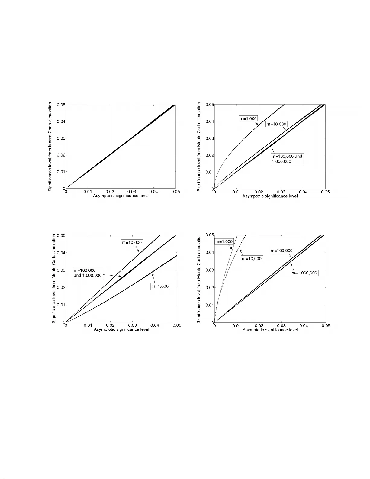
χ 2 and classical exact tests often wild l y misrep ort signiﬁcance; t h e remedy lies i n computers Willi a m P erkins ∗ , Mark T ygert † , and Rac hel W ard ‡ August 14, 2 0 18 Abstract If a discrete probabilit y distribu tion in a model b eing te sted for go o dness-of-ﬁt is not close to uniform, th en forming the P earson χ 2 statistic can in v olv e d ivision b y nearly zero. This often leads t o serious trouble in practice — ev en in the absence of roun d-oﬀ errors — a s the pr esen t article illus tr ates via n umerous examp les. F ortunately , with the no w widespread a v ailabilit y of compu ters, a v oiding all the trouble is simple and easy: without th e problematic d ivision by n early zero, the actual v alues ta k en by goo d ness- of-ﬁt sta tistics are n ot h umanly inte rpretable, bu t blac k-b o x computer programs can rapidly calc ulate their precise signiﬁ cance. ∗ Suppo rted in par t by NSF Grant OISE-073 0136 and an NSF Postdo ctora l Resea r ch F ellowship † Suppo rted in par t by a Research F ellowship from the Alfred P . Sloan F oundation ‡ Suppo rted in par t by an NSF Postdoc to ral Research F ello wship and a Dona ld D. Harring ton F acult y F ellowship 1 Con ten ts 1 In tro duction 3 2 Deﬁnitions of the test statistics 5 3 Hyp othesis t est s with parameter estimation 6 4 Data analysis 9 4.1 Syn thetic examples . . . . . . . . . . . . . . . . . . . . . . . . . . . . . . . . 9 4.2 Zipf ’s p ow er la w of word frequencies . . . . . . . . . . . . . . . . . . . . . . 10 4.3 A P oisson law for radioactiv e decay s . . . . . . . . . . . . . . . . . . . . . . 15 4.4 A P oisson law for coun ting with a hæmacytometer . . . . . . . . . . . . . . . 15 4.5 A Hardy-W ein b erg law for Rhesus blo o d groups . . . . . . . . . . . . . . . . 17 4.6 Symmetry b et w een the self-rep orted health assessm en ts of foreign- and US- b orn Asian Americans . . . . . . . . . . . . . . . . . . . . . . . . . . . . . . 20 4.7 A mo diﬁed geometric law for the sp ecies of butterﬂies . . . . . . . . . . . . . 23 4.8 A mo diﬁed geometric law for religious aﬃliat ions . . . . . . . . . . . . . . . 23 5 The p ow er and eﬃciency of t he ro ot-mean-square 27 5.1 Examples without para meter estimation . . . . . . . . . . . . . . . . . . . . 28 5.1.1 A simple, illustrativ e example . . . . . . . . . . . . . . . . . . . . . . 28 5.1.2 T runcated p ow er-la ws . . . . . . . . . . . . . . . . . . . . . . . . . . 30 5.1.3 Additional truncated p o w er-la ws . . . . . . . . . . . . . . . . . . . . 31 5.1.4 Additional truncated p o w er-la ws, rev ersed . . . . . . . . . . . . . . . 32 5.1.5 A ﬁnal example with fully sp eciﬁed truncated p ow er-la ws . . . . . . . 33 5.1.6 Mo diﬁed P oisson distributions . . . . . . . . . . . . . . . . . . . . . . 34 5.1.7 A truncated p o w er-la w and a t r uncated geometric distribution . . . . 3 5 5.2 Examples with parameter estimation . . . . . . . . . . . . . . . . . . . . . . 36 5.2.1 A truncated p o w er-la w and a t r uncated geometric distribution . . . . 3 6 5.2.2 A rebinned geometric distribution and a truncated p ow er-la w . . . . 37 5.2.3 T runcated shifted Poisson distributions . . . . . . . . . . . . . . . . . 38 5.2.4 Mo diﬁed P oisson distributions . . . . . . . . . . . . . . . . . . . . . . 39 5.2.5 An example with a uniform tail . . . . . . . . . . . . . . . . . . . . . 40 5.2.6 Another example with a uniform tail . . . . . . . . . . . . . . . . . . 41 5.2.7 A mo del with an integer-v alued para meter . . . . . . . . . . . . . . . 42 5.2.8 T runcated p ow er-la ws parameterized with a p erm utation . . . . . . . 4 3 5.2.9 Another mo del parameterized with a p erm utation . . . . . . . . . . . 44 5.2.10 A mo del with t w o parameters . . . . . . . . . . . . . . . . . . . . . . 45 A Additional plots of p ow er and eﬃciency 46 B Con v ergence to asymptotic lev els 56 References 62 2 1 In tro duc t ion A basic task in statistics is to a scertain whether a giv en set of indep enden t and iden tically distributed ( i.i.d.) dra ws do es not come from a g iv en “mo del,” where the mo del may consist of either a single fully sp eciﬁed probabilit y distribution or a parameterized fa mily of prob- abilit y distributions. The presen t pap er concerns the case in which the draws are discrete random v ariables, taking v alues in a ﬁnite or coun table set. In accordance with the standard terminology , w e will r efer to the p ossible v alues of the discrete random v ariables as “bins” (“categories,” “cells,” and “classes” are common synon yms for “ bins”). A natural approa c h to ascertaining whether the i.i.d. draws do not come from the mo del uses a ro o t - mean-square statistic. T o construct this statistic, w e estimate the probabilit y distribution o v er the bins using the given i.i.d. dra ws, and then measure the ro ot-mean-square diﬀerence b etw een this empirical distribution and the mo del distribution; see, for example, [17], page 123 of [21], or Section 2 b elo w. If the dra ws do in fact arise from the mo del, then with high probability this ro o t - mean-square is not larg e. Th us, if the ro ot-mean-square statistic is large, then we can b e conﬁden t that the draw s do not ar ise from the mo del. T o quantify “large” and “conﬁden t,” let us denote b y x the v a lue of t he ro ot-mean-square for the giv en i.i.d. dra w s; let us denote by X the ro ot-mean-square statistic constructed for diﬀeren t i.i.d. draws that deﬁnitely do in fa ct come from the mo del (if the mo del is parameterized, then w e draw from the distribution corresponding to the parameter give n b y a maximum-lik eliho o d estimate for the exp erimen tal data) . The signiﬁcance lev el α is then deﬁned to b e the probabilit y that X ≥ x (viewing X — but not x — as a rando m v ariable). The conﬁdence lev el that the giv en i.i.d. dra ws do not arise from the mo del is the complemen t of the signiﬁcance leve l, namely 1 − α . (See Remark 1.2 concerning our use of the term “ signiﬁcance lev el” a s synon ymous with the alternative term “ p - v alue.”) No w, the signiﬁcance lev els for the simple ro ot-mean-square statistic can b e diﬀerent functions of x f or diﬀeren t mo del pr o babilit y distributions. T o av oid this seeming incon- v enience asymptotically (in the limit of large n um bers of draw s), K. Pe arson replaced the uniformly w eigh ted mean in the ro o t-mean-square with a w eigh ted a v erage; the w eigh ts are the recipro cals of the mo del probabilities a sso ciat ed with the v arious bins. This pro duces the classic χ 2 statistic — see, for example, [14] or formu la (2) b elow. How ev er, when mo del probabilities can b e small (relativ e to others in the same distribution), this w eigh ted a v erage can in v olv e division by nearly zero. As demonstrated below, dividing by nearly zero sev erely restricts t he statistical p ow e r of χ 2 — ev en in the absence of round-oﬀ errors — esp ecially when dividing by nearly zero for eac h of man y bins. Moreov er, this problem arises whether or not ev ery bin contains sev eral draws (see Remark 1.1). The main thesis of the presen t article is that using only the classic χ 2 statistic is no longer appropriate, that certain alternativ es are far superio r no w that computers are widely a v ailable. W e demonstrate b elo w t ha t the simple ro ot-mean-square, used in conjunction with the log–likelihoo d- ratio “ G 2 ” go o dness -of-ﬁt statistic, is g enerally preferable to the classic χ 2 statistic. (The lo g–lik eliho o d-ratio also in v olves division by nearly zero, but temp ers this somew hat by taking a logarithm.) W e do not make any claim that this is the b est p ossible a lt ernat iv e. In fact, the discrete Kolmogorov-Smirno v statistic ( or one of its v a rian ts, suc h as t he discrete Kuip er statistic — see, for example, [3] o r [5]) can b e more p o w erful than the ro ot- mean-square in certain circumstances; in an y case, the discrete Ko lmogoro v- 3 Smirno v statistic and the ro ot-mean-square are similar in man y w a ys, a nd complemen tary in ot hers. W e fo cus on the ro ot-mean-square largely b ecause it is so simple and easy to understand; for example, computing the conﬁdence lev els of the r o ot-mean-square in the limit o f la rge n um b ers of draw s is tr ivial, ev en when estimating contin uous parameters via maxim um-lik elihoo d metho ds (se e [1 5] a nd [16]). F urthermore, the classic χ 2 statistic is just a weigh ted v ersion of the ro ot - mean-square, facilitating their comparison. Finally , χ 2 and the ro ot -mean-square coincide when the mo del distribution is uniform. Please note that all statistical tests rep orted in the presen t pap er (including those inv olv- ing the χ 2 statistic) are exact; w e compute signiﬁcance lev els via Mon te-Carlo sim ulations pro viding guaran teed erro r b ounds (see Section 3 b elow ). In all n umerical results rep orted b elo w, we generated random n um bers via the C programming language pro cedure given on page 9 of [13], implemen ting the recommended complemen tary m ultiply with carry . T o b e sure, the problem with χ 2 is neither subtle nor esoteric. F or a particularly rev ealing example, see Subsection 4.5 b elo w. Appropriate rebinning to unifo r mize the probabilities asso ciated with the bins can miti- gate muc h of the problem with χ 2 . Y et rebinning is a black art that is liable to improp erly inﬂuence the result of a go o dness-of-ﬁt test. Moreov er, rebinning requires careful extra w ork, making χ 2 less easy-to-use. A principal adv antage of the ro ot-mean-square is that it do es not require any rebinning; indeed, the ro ot-mean-square is most p o w erful without an y rebinning. Remark 1.1. In man y of our examples, t here is a bin for whic h the exp ected n um ber of dra ws is v ery small under the mo del. Please note that, altho ug h it is nat ural for the exp ected n um bers of dra ws fo r some bins to be v ery small, esp ecially when the mo del has many bins, the a dv antage o f the ro ot - mean-square ov er χ 2 is substantial eve n when the expected n um b er of dra ws is at least ﬁv e for ev ery bin; see, for example, Subsection 5.1.1 or Subsection 5.2.6. Remark 1.2. Please b ew are that w e treat “signiﬁcance lev el” as synony mous with the alternativ e term “ p -v alue.” These tw o terms are not exactly the same in the classical ter- minology . Ho w ever, the o lder concept of “signiﬁcance leve l” is no longer ve ry relev ant, due to the pr o liferation of computer tec hnology; there is no longer m uc h reason to calculate and store tables of thresholds for go o dness-of-ﬁt statistics at arbitrarily ﬁxed signiﬁcance lev els — w e can now compute “ p -v a lues” on the ﬂy , as needed. The ob jectiv e o f a signiﬁcance test is not really to accep t or reject a h ypothesis at some arbitrary threshold of signiﬁcance , but instead to pro vide signiﬁcance lev els that can inform statisticians’ f urt her analysis. Remark 1.3. Go o dness-of-ﬁt tests are probably most useful in practice not for ascertaining whether a mo del is correct or not, but for determining whethe r the discrepancy b et w ee n the mo del and exp erimen t is la r g er than exp ected random ﬂuctuations. While mo dels outside the ph ysical sciences t ypically are not exactly correct, t esting the v alidit y of using a mo del for virtually any purp ose requires kno wing whether observ ed discrepancies are due to inac- curacies o r inadequacies in the mo dels or (on the contrary) could b e due to chance arising from necessarily ﬁnite sample sizes. Th us, go o dness -of-ﬁt t ests are critical ev en when the mo dels are not supp osed to b e exactly corr ect, in order to gauge the size of t he una v oidable random ﬂuctuations. F or further clariﬁcation, see [10] and the remark ably extensiv e t itle of the original a rticle [14] that in tro duced the χ 2 test for go o dness-of-ﬁt. 4 Remark 1.4. Com bining the ro ot-mean-square metho dology and t he statistical b o otstrap (see, for example, [6]) should pro duce a test for whether t w o separate sets of draws arise from the same o r from diﬀeren t distributions, when eac h set is tak en i.i.d. from some (unsp eciﬁed) distribution; the tw o distributions asso ciated with the sets ma y diﬀer. This is related to testing for asso ciation/indep endence in contingency -tables/cross-tabulations that ha v e only t w o ro ws. 2 Deﬁniti o ns of the test statist ics In this section, w e review the deﬁnitions of four go o dness-of-ﬁt statistics — the ro ot- mean- square, χ 2 , the lo g–lik eliho o d-ratio or G 2 , and the F reeman-T uk ey or Hellinger dis tance. The latter three statistics are the b est-kno wn mem b ers of the standa r d Cressie-Read p ow er- div ergence family (see, fo r example, [17 ]). W e use p 1 , p 2 , . . . , p n − 1 , p n to denote the exp ected fractions of m i.i.d. dra ws fa lling in n bins, n um b ered 1, 2, . . . , n − 1, n , resp ectiv ely , a nd w e use q 1 , q 2 , . . . , q n − 1 , q n to denote t he observ ed fractions of the m dra ws falling in the resp ectiv e bins. That is, p 1 , p 2 , . . . , p n − 1 , p n are t he probabilities asso ciated with the resp ectiv e bins in the m o del distribution, whereas q 1 , q 2 , . . . , q n − 1 , q n are the f ractions o f the m draws falling in the resp ectiv e bins when we tak e the dra ws from a distribution that ma y diﬀer fr o m the mo del — their actual distribution. Speciﬁcally , if i 1 , i 2 , . . . , i m − 1 , i m are the observ ed i.i.d. dra ws, then q k is 1 m times the num b er of i 1 , i 2 , . . . , i m − 1 , i m falling in bin k , for k = 1, 2, . . . , n − 1, n . If the mo del is pa rameterized b y a parameter θ , then the probabilities p 1 , p 2 , . . . , p n − 1 , p n are functions of θ ; if the model is fully sp eciﬁed, then w e can view the probabilities p 1 , p 2 , . . . , p n − 1 , p n as constant as functions of θ . W e use ˆ θ to denote a maxim um-lik eliho o d estimate of θ obta ined from q 1 , q 2 , . . . , q n − 1 , q n . With this notation, the ro ot- mean-square statistic is X = v u u t 1 n n X k =1 ( q k − p k ( ˆ θ )) 2 . (1) W e use t he designation “ro ot-mean-square” to refer to X . The classical P earson χ 2 statistic is χ 2 = m n X k =1 ( q k − p k ( ˆ θ )) 2 p k ( ˆ θ ) , (2) under the con v en tio n that ( q k − p k ( ˆ θ )) 2 /p k ( ˆ θ ) = 0 if p k ( ˆ θ ) = 0 = q k . W e use the standar d designation “ χ 2 ” to refer t o χ 2 . The log– likelihoo d-ratio or “ G 2 ” statistic is G 2 = 2 m n X k =1 q k ln q k p k ( ˆ θ ) ! , (3) under t he conv ention that q k ln( q k /p k ( ˆ θ )) = 0 if q k = 0. W e use the common designation “ G 2 ” to r efer to G 2 . 5 The F reeman-T ukey or Hellinger-distance statistic is H 2 = 4 m n X k =1  √ q k − q p k ( ˆ θ )  2 = 4 m n X k =1 " ( q k − p k ( ˆ θ )) 2   √ q k + q p k ( ˆ θ )  2 # . (4) W e use t he w ell-kno wn designation “F reeman-T uke y” to refer t o H 2 . In the limit that the n um b er m of draws is large, the distributions of χ 2 deﬁned in ( 2 ), G 2 deﬁned in (3), and H 2 deﬁned in (4) are all the same when the actual underlying distribu- tion of the draws comes from the model (see, for example, [1 7 ]). Ho w ev er, when the n um b er m of dra ws is not larg e, then their distributions can diﬀer substan tia lly . In a ll our data and p o w er analyses, w e compute conﬁdence lev els via Mon te-Carlo sim ulations, without relying on the num b er m of draws to b e larg e. 3 Hyp ot hesis tests wit h parameter es timation In this section, w e discuss the t esting of hy p otheses in v olving para meterized mo dels: Giv en a family p ( θ ) o f pro babilit y distributions parameterized by θ , and giv en observ ed i.i.d. draws from some actual underly ing (unkno wn) distribution ˜ p , we would like to test t he h y p othesis H ′ 0 : f o r some θ , ˜ p = p ( θ ) , (5) against the alternativ e H ′ 1 : f o r all θ , ˜ p 6 = p ( θ ) . (6) Giv en only ﬁnitely man y dra ws, the signiﬁcance lev el for suc h a test w ould ha v e to b e inde- p enden t of the parameter θ , since the prop er v alue for θ is unknown ( θ is kno wn as a n uisance parameter). Unfortunately , it is not clear ho w to devise suc h a test when the probability distributions are discrete. None o f the standard metho ds ( including χ 2 , t he log–lik eliho o d- ratio, the F reeman-T uk ey/Hellinger distance, and other p o w er- div ergence statistics) pro duce signiﬁcance lev els t ha t a re indep enden t of the parameter θ . Some metho ds do pro duce sig- niﬁcance lev els that are indep enden t of θ in the limit of la r ge n um b ers of dr aws, but this is not esp ecially useful, since in the limit of large num b ers of draws any a ctual parameter θ w ould b e almost surely known an yw a y (see App endix B f or further elab o ration). In the presen t pap er, we test the signiﬁcance of assuming H 0 : ˜ p = p ( ˆ θ ) for the particular observ ed v a lue of ˆ θ , (7) where ˆ θ is a maxim um-lik eliho o d estimate of θ ; tha t is, H 0 is the h ypot hesis that ˜ p = p ( ˆ θ ) for the v alue of ˆ θ asso ciated with the single realization of the exp erimen t that w as measured (subseque n t rep etitions of the exp erimen t, including those considered when calculating the signiﬁcance lev el as in Remark 3.3, can yie ld diﬀeren t estimates of the parameter, ev en though the rep etitions’ actual distribution ˜ p is the same). O f course, the a ccuracy of the estimate ˆ θ g enerally impro v es as the num b er of dra ws increases; in fact, testing (5) and testing (7) are asymptotically equiv alen t, in the limit o f large n um b ers of draw s (see [16]). As testing the h ypothesis H ′ 0 deﬁned in (5) do es not seem to b e feasible in general when the probability distributions are discrete and there are more than just a few bins, we f o cus on testing t he closely related assumption H 0 deﬁned in (7). The latter is more r elev an t 6 for many applicatio ns, anyw ays — plots t ypically display the particular ﬁtted distribution in (7); in terpreting such plots naturally in v olv es (7). All tests o f the presen t pap er concern the signiﬁcance of assuming H 0 deﬁned in (7) (if the mo del is fully sp eciﬁed, then the probability distribution p ( θ ) is the same for all θ ). Please b e sure to b ear in mind Remark 1.3 of Section 1. Remark 3.1. Another means of handling n uisance parameters is to test the hy p othesis H ′′ 0 : ˜ p = p ( ˆ θ ) for all p ossible r ealizatio ns of t he exp erimen t; (8) that is, H ′′ 0 is the h yp othesis that ˜ p = p ( ˆ θ ) and tha t p ( ˆ θ ) alw a ys take s exactly the same v alue during repetitio ns of the exp erimen t. The assumption that (8) is true see ms to b e more extreme, a more substan tial departure fro m (5 ) , than (7 ). Nev ertheless, testing (8) is standard; see, for example, Section 6 of [4 ]. Assuming (8) amoun ts to conditioning (5 ) on a statistic that is minimally suﬃcien t fo r estimating θ ; computing the asso ciated signiﬁcance lev els is not alw a ys trivial. T esting the signiﬁcance of assuming (7 ) w ould seem to b e more aprop os in pra ctice for applications in whic h the exp erimen tal design do es not enforce that rep eated exp erimen ts alwa ys yield the same v alue for p ( ˆ θ ). Remark 3.2. The par a meter θ can b e integer-v alued, real- v alued, complex-v alued, v ector- v alued, matrix-v alued, or an y combination of the man y p ossibilities . F or instance, when we do no t kno w the prop er or dering of the bins a priori, we must include a para meter that con tains a p erm utation (or p erm utation matrix) specifying the order of the bins; maxim um- lik elihoo d estimation then en tails sorting the mo del a nd all empirical frequencie s (whether exp erimental or simulated) — see Subse ction 4.2 for details. With Remark 3 .3, w e need not con template how man y degrees of freedom are in a p ermutation. Remark 3.3. T o compute the lev el of signiﬁcance of assum ing (7), w e can use Monte-Carlo sim ulations (v ery similar to those in [3]). First, w e estimate the par a meter θ from t he m g iv en exp erimental draw s, obtaining ˆ θ , and then calculate the statistic under consideration ( χ 2 , G 2 , F reeman-T ukey , or the ro ot-mean-square), using the g iv en data and taking the mo del distribution t o b e p ( ˆ θ ). W e then run many sim ulations. T o conduct a single sim ulation, w e p erform the follow ing three-step pro cedure: 1. w e generate m i.i.d. dra ws a ccording to the mo del distribution p ( ˆ θ ), where ˆ θ is the estimate calculated from the exp erimen tal data, 2. w e estimate the pa r ameter θ from the data generated in Step 1, obta ining a new estimate ˜ θ , and 3. w e calculate the statistic under consideration ( χ 2 , G 2 , F reeman-T uk ey , or the ro ot- mean-square), using the data g enerated in Step 1 and taking the mo del distribution to b e p ( ˜ θ ), where ˜ θ is the estimate calculated in Step 2 from the data generated in Step 1. After conducting many suc h sim ulations, we may estimate the conﬁdence lev el for reject- ing (7) as the fraction of the statistics calculated in Step 3 that ar e less than the statistic calculated from the empirical data. (Recall t hat a signiﬁcance level of α is the same as a conﬁdence lev el of 1 − α .) The accuracy of the estimated conﬁdence lev el is inv ersely pro p or- tional to the square r o ot of the n um b er of sim ulations conducted; for details, see Remark 3.4 b elo w. This pro cedure works since, b y deﬁnition, the conﬁdence lev el is the probability that 7 d               Q 1 Q 2 . . . Q n − 1 Q n        ,        p 1 (Θ) p 2 (Θ) . . . p n − 1 (Θ) p n (Θ)               < d               q 1 q 2 . . . q n − 1 q n        ,        p 1 ( ˆ θ ) p 2 ( ˆ θ ) . . . p n − 1 ( ˆ θ ) p n ( ˆ θ )               , (9) where • n is the num b er of all p ossible v alues that the dra ws can take, • d is the measure of the discrepancy b etw een t w o probability distributions o v er n bins (i.e., b et w ee n t w o v ectors eac h with n entries) that is associat ed with the statistic under consideration ( d is the Euclidean distance for the ro o t-mean-square, a w eigh ted Euclidean distance for χ 2 , the Hellinger distance for the F reeman-T uk ey statistic, and the relativ e entrop y — the K ullba ck-Leibler div ergence — for the log–like liho o d-r a tio), • q 1 , q 2 , . . . , q n − 1 , q n are the f r a ctions of t he m give n experimen tal dra ws falling in the resp ectiv e bins, • ˆ θ is the estimate of θ obta ined from q 1 , q 2 , . . . , q n − 1 , q n , • Q 1 , Q 2 , . . . , Q n − 1 , Q n are the f ractions o f m i.i.d. dr aws falling in the resp ectiv e bins when taking the dra ws fro m the distribution p ( ˆ θ ) assumed in (7), a nd • Θ is the estimate of the parameter θ obtained f rom Q 1 , Q 2 , . . . , Q n − 1 , Q n (note that Θ is not necessarily alw a ys equal to ˆ θ : ev en under the nu ll h ypo thesis, rep etitions of the exp erimen t could yield diﬀeren t estimates of the parameter; see also Remark B.2). When t a king the probabilit y that (9) o ccurs, only the left-hand side is random — we regard the left-hand side of (9) as a random v ariable and the right-hand side as a ﬁxed num b er determined via the exp erimen tal data . As with any probability , to compute the probability that (9) o ccurs, w e can calculate man y indep enden t realizations of the r a ndom v ariable and observ e that the fraction whic h satisfy (9) is a g o o d appro ximation to the probability when the n um ber of realizatio ns is large; Remark 3.4 details the accuracy of t he a ppro ximation. (The pro cedure in the presen t remark follows this prescription to estimate conﬁdence lev els.) Remark 3.4. The standard erro r of the estimate from Remark 3.3 for an exact signiﬁcance lev el of α is p α (1 − α ) /ℓ , where ℓ is the n um ber of Mon te-Carlo sim ulations conducted to pro duce the estimate. Indeed, eac h simulation has probability α of pro ducing a statistic t ha t is greater than or equal to the statistic corr esp onding to an exact signiﬁcance lev el of α . Since the sim ulations are all indep enden t, the num b er of the ℓ sim ulations that pro duce statistics greater t han or equal to that corresp onding to lev el α f ollo ws the binomial distribution with ℓ trials and probabilit y α of succes s in eac h trial. The standard deviation of the n um b er of sim ulations whose statistics are greater than or equal to that corresp onding to lev el α is therefore p ℓα (1 − α ), and so the standard deviation of the fr action of the sim ulations pro ducing suc h statistics is p α (1 − α ) /ℓ . Of course, the fraction itself is the Mon te-Carlo estimate of the exact signiﬁcance lev el (w e use this estimate in place of the unkno wn α when calculating the standard error p α (1 − α ) /ℓ ). 8 4 Data analysis In this section, w e use sev eral data sets to inv estigate t he p erformance of go o dness-of-ﬁt statistics. The ro ot-mean-square generally p erforms m uc h b etter than the classical statistics. W e tak e the p osition that a user of statistics should not ha v e to w orry ab out rebinning; w e discuss rebinning only brieﬂy . W e compute all signiﬁcance leve ls via Mon te Carlo as in Remark 3.3 ; Remark 3.4 details the guaranteed accuracy of the computed signiﬁcance lev els. 4.1 Syn thetic examples T o b etter explicate t he p erformance of the g o o dness-of-ﬁt statistics, w e ﬁrst a nalyze some to y examples. W e consider the mo del distribution p 1 = 1 4 , (10) p 2 = 1 4 , (11) and p k = 1 2 n − 4 (12) for k = 3, 4, . . . , n − 1, n . F or the empirical distribution, w e ﬁrst use m = 20 dra ws, with 15 in the ﬁrst bin, 5 in the second bin, and no draw in an y other bin. This data is clearly unlik ely to arise from the mo del sp eciﬁed in (10)–(12), but w e w ould like to see exactly how w ell the v arious go o dness -of-ﬁt statistics detect the ob vious discrepancy . Figure 1 plots the signiﬁcance lev els f o r testing whether the empirical data arises from the mo del sp eciﬁed in (10)–(12). W e computed the signiﬁcance lev els via 4,000,0 00 Monte -Carlo sim ulations (that is, 4,000,000 p er empirical signiﬁcance lev el b eing ev aluated), with each sim ulation ta king m = 20 draws from the mo del. The ro o t-mean-square consisten tly and with extremely high conﬁdence rejects the h yp othesis that the data a rises from the mo del, whereas the classical statistics ﬁnd less and less evidence for rejecting t he hypothesis as the n um ber n of bins increase s; in fact, the signiﬁcance lev els for the classical statistics get ve ry close to 1 as n increases — the discrepancy of ( 12) from 0 is usually less than the discrepancy of (12) from a typical realization drawn from the mo del, since under the mo del the sum of the exp ected num b ers of dra ws in bins 3, 4, . . . , n − 1, n is m/ 2. Figure 1 demonstrates that the ro ot- mean-square can b e muc h more p o w erful than t he classical statistics, rejecting with nearly 100% conﬁdence while the classic al statistics repo r t nearly 0% conﬁdence for rejection. Moreo v er, the classical statistics can rep ort signiﬁcance lev els v ery close to 1 ev en when the data manifestly do es not ar ise fro m the mo del. (Inci- den tally , the mo del for smaller n can b e view e d as a rebinning o f the mo del for lar ger n . The classical stat istics do reject the mo del for smaller n , while asserting for lar ger n that there is no evidence for r ejecting the mo del.) The p erfo rmance of the classical stat istics displa ys a drama t ic dep endence on the n um ber ( n − 2) of unlik ely bins in the mo del, ev en though the dat a are the same for all n . This suggests a sure-ﬁre sch eme for supp orting any mo del (no matter ho w in v alid) with arbitra rily high signiﬁcance: just app end enough irrelev an t, more or less uniformly improbable bins to the mo del, and then rep o r t the signiﬁcance lev els 9 1E-7 1E-6 1E-5 1E-4 1E-3 1E-2 1E-1 1E-0 10 20 30 40 50 60 70 80 90 100 significance level number (n) of bins χ 2 G 2 root-mean-square Freeman-Tukey Figure 1: Signiﬁcance lev els for the h yp othesis that the mo del (10)–(12) agrees with the data of 15 draws in the ﬁrst bin, 5 dra ws in the second bin, and no draw in an y other bin for the classical go o dness-of-ﬁt statistics. In con trast, the ro ot- mean- square robustly and reliably rejects t he in v alid mo del, indep enden tly of the size of the mo del. W e will see in the follow ing section that the classic Zipf p o w e r law behav es similarly . F or another example, w e again consid er the mo del speciﬁed in (10)–(12). F or the empir- ical distribution, w e now use m = 9 6 draw s, with 3 6 in the ﬁrst bin, 1 2 in the second bin, 1 eac h for bins 3, 4, . . . , 4 9 , 5 0, and no draw in an y other bin. As b efore, this data clearly is unlik ely to arise from the mo del sp eciﬁed in (10)–(12), but w e w ould lik e t o see exactly ho w w ell the v ario us go o dness-of- ﬁt statistics detect the ob vious discrepancy . Figure 2 plots the signiﬁcance lev els for testing whether the empirical data arises from the mo del sp eciﬁed in (10)–(12). W e computed the signiﬁcance leve ls via 160,00 0 Monte- Carlo sim ulations (that is, 160,00 0 p er empirical signiﬁcance lev el b eing ev aluated), with eac h simulation taking m = 96 draws from the mo del. Y et again, t he ro o t-mean-square consisten tly and conﬁdently rejec ts the hypothesis that the data arises from the mo del, whereas the classical statistics ﬁnd little evidence for rejecting the manifestly in v alid mo del. 4.2 Zipf ’s p o w er la w of w ord frequencies Zipf p opularized his ep onymous law by analyzing four “c hief sources of statistical data re- ferred to in the main text [23]” (this is a quotation fro m the “Notes and Reference s” section — page 311 — of [23]); in [23], t he c hief source for the English language is [7]. W e revisit the data from [7] in the presen t subsection to a ssess the p erformance of the g o o dness-of-ﬁt statistics. W e ﬁrst a nalyze List 1 of [7], whic h consists of 2,89 0 diﬀeren t English w ords, suc h that 10 1E-4 1E-3 1E-2 1E-1 1E-0 100 200 300 400 500 600 700 800 900 1000 significance level number (n) of bins χ 2 G 2 root-mean-square Freeman-Tukey Figure 2: Signiﬁcance lev els for the hypothesis that the mo del (10)–(12) agrees with the data of 36 draws in the ﬁrst bin, 12 draws in the second bin, 1 dra w eac h in bins 3, 4, . . . , 49, 50, and no draw in an y ot her bin there a r e 13,825 w ords in tota l coun ting rep etitions; the w ords come fro m the Buﬀalo Sunda y News of August 8, 19 09. W e randomly c ho ose m = 10 ,000 of the 1 3,825 w ords t o obtain a corpus of m = 10,000 draws ov er 2,89 0 bins. Figure 3 plots the f requencies of the diﬀeren t w ords when sorted in rank order (so tha t the frequencies a re nonincreasing). Using go o dness- of-ﬁt statistics we test the signiﬁcance of the (n ull) h ypothesis that the empirical draws actually arise fr om the Z ipf distribution p k ( θ ) = C 1 θ ( k ) (13) for k = 1, 2, . . . , n − 1, n , where θ is a p ermutation of the integers 1, 2, . . . , n − 1, n , and C 1 = 1 P n k =1 1 /k ; (14) w e estimate the permutation θ via maximum-lik eliho o d metho ds, that is, b y sorting the frequencies: ﬁrst w e c ho ose k 1 to b e the num b er o f a bin containing the g r eat est n um b er of dra ws among all n bins, then w e c ho ose k 2 to b e the n um b er of a bin con taining t he greatest n um ber of draws among the remaining n − 1 bins, then we c hoo se k 3 to b e the n um b er o f a bin containing the greatest among the remaining n − 2 bins, and so on, and ﬁnally w e ﬁnd θ suc h that θ ( k 1 ) = 1, θ ( k 2 ) = 2, . . . , θ ( k n − 1 ) = n − 1, θ ( k n ) = n . W e hav e to obta in the ordering θ from the dat a via suc h sorting since w e do no t know the prop er or dering a priori. Similarly , w e do not kno w the prop er v alue of the num b er n of bins, so in Figure 4 w e plot signiﬁcance lev els (eac h computed via 40,000 Monte-Carlo sim ulations) for v arying v alues of 11 n ; altho ugh List 1 of [7] inv olves o nly 2,890 distinct w ords, we m ust a lso include bins for w ords that did not app ear in t he origina l list, words whose frequencies are zeros fo r List 1 of [7]. Note that Figure 4 display s the signiﬁcance lev els with n = 2,890 fo r reference, ev en though n m ust b e indep enden t of the data, and so n m ust b e substan tially larger t ha n 2,890 in order for the a ssumptions of go o dness-of-ﬁt testing to hold. With resp ect to testing go o dness -of-ﬁt , t he n um ber n of bins is the n um b er o f words in the dictionary from whic h List 1 of [7] w as draw n. It is not clear a priori whic h dictionary is appro priate. F ortunately , the signiﬁcance lev els for the ro ot-mean- square are alwa ys 0 to sev eral digits of accuracy , indep enden t of the v alue of n — the ro ot-mean-square determines that List 1 do es not follow the classic Zipf distribution (deﬁned in (1 3) and (14)) f or any n . In con trast, the signiﬁcance lev els for the classical statistics v ary wildly dep ending on the v alue o f n . In fact, for any of the classical statistics, and for any prescribed n um b er α b et w een 0.05 and 0.9 5, there is at least one v alue of n b etw een 4,000 and 40 ,000 suc h that the signiﬁcance lev el is α . Th us, without kno wing the prop er size of the dictionary a priori, the classical stat istics are meaningless. Unsurprisingly , analyzing L ist 5 of [7] pro duces results analogous to those rep orted ab ov e for L ist 1. List 5 consists of 6,002 diﬀeren t English w ords, suc h that there are 43,9 89 w ords in total coun ting rep etitions; t he w ords come from amalgama t ing Lists 1–4 of [7]. W e ra ndomly c ho ose m = 20 ,0 00 of the 43 ,989 w ords to obtain a corpus of m = 20,000 draw s o v er 6,002 bins. Figure 5 plots the f r equencies of the diﬀerent w ords when sorted in rank o rder (so that the frequencies a re nonincreasing). Again w e do not kno w the prop er v alue of the num b er n of bins, so in Figure 6 we plot signiﬁcance lev els (eac h computed via 40,000 Monte-Carlo sim ulations) for v arying v alues of n ; altho ugh List 5 of [7] inv olves o nly 6,002 distinct w ords, we m ust a lso include bins for w ords that did not app ear in t he origina l list, words whose frequencies are zeros fo r List 5 of [7]. Please note that F ig ure 6 displa ys the signiﬁcance lev els with n = 6,002 for reference , ev en though n m ust b e indep enden t of the data, and so n mus t b e substan tially larger than 6,002 in order for the assumptions of go o dness -of-ﬁt testing to hold. Comparing Figures 4 and 6 sho ws that the ab o v e remarks ab out List 1 p ertain to the analysis of the larger List 5, to o. Once ag ain, without kno wing the prop er size of the dictionar y a prio ri, the classical statistics are meaningless, whereas t he ro ot- mean-square is v ery p ow erful. In terestingly , b y in tro ducing para meters θ 1 , θ 2 , and θ 3 to ﬁt p erfectly the bins containing the t hree greatest n um bers of draws, a truncated p ow er-law b ecomes a go o d ﬁt for the corpus of 20 ,000 words dra wn ra ndomly from L ist 5 of [7], with the n um b er n of bins set to 7,50 0. Indeed, let us consider the mo del p k ( θ 0 , θ 1 , θ 2 , θ 3 , θ 4 ) =        θ 1 , θ 0 ( k ) = 1 θ 2 , θ 0 ( k ) = 2 θ 3 , θ 0 ( k ) = 3 C / ( θ 0 ( k )) θ 4 , θ 0 ( k ) = 4 , 5 , . . . , 7499 , 7500 , (15) where C = C θ 1 ,θ 2 ,θ 3 ,θ 4 = 1 − θ 1 − θ 2 − θ 3 P 7500 k =4 1 /k θ 4 , (16) with θ 0 b eing a p erm utation of the inte gers 1, 2, . . . , 74 99, 75 00, and θ 1 , θ 2 , θ 3 , θ 4 b eing nonnegativ e real nu m b ers; w e estimate θ 0 , θ 1 , θ 2 , θ 3 , θ 4 via maxim um-lik eliho o d metho ds, 12 0.1 1 10 100 1000 10000 1 10 100 1000 number of occurrences bin number Figure 3: Numbers of o ccurrences of the v arious w ords (one bin for eac h distinct w ord) in a corpus of 10,000 random dra ws from L ist 1 of [7 ] determining θ 0 b y sorting as discussed ab ov e, and setting θ 1 , θ 2 , and θ 3 to b e the three greatest relative frequencies. This mo del ﬁts the empirical data exactly in the bins whose probabilities under the model are θ 1 , θ 2 , and θ 3 — there will b e no discrepancy b et w een the data and the mo del in those bins — so that these bins do not con tribute to an y g o o dness- of-ﬁt statistic, aside from altering the n um b er of draws in the remaining bins. O f the 20,000 total draw s in the giv en exp erimen tal dat a, 1 6 ,486 do not fall in the bins asso ciated with the three most frequen tly o ccurring words. The maxim um-lik eliho o d estimate of the p ow er-law exp o nen t θ 4 for the exp erimen tal data turns out to b e ab out 1.04 8 4. F or the mo del deﬁned in (15) and ( 1 6), the signiﬁcance lev els calculated via 4 ,000,000 Mon te-Carlo sim ulations are • χ 2 : .510 • G 2 : .998 • F reeman-T uk ey: 1.000 • ro ot- mean-square: .587 Th us, all four statistics indicate that the truncated p o w er- la w mo del deﬁned in (15) and (16) is a go o d ﬁt. This is in accord with Figure 5, in whic h all but the three greatest frequencie s app ear to follow a truncated p ow er-la w. 13 0 0.2 0.4 0.6 0.8 1 10000 20000 30000 40000 significance level number (n) of bins χ 2 root-mean-square Freeman-Tukey G 2 2890 Figure 4: Signiﬁcance lev els for the data plotted in Figure 3 to fo llo w the Zipf distribution 0.1 1 10 100 1000 10000 1 10 100 1000 number of occurrences bin number Figure 5: Numbers of o ccurrences of the v arious w ords (one bin for eac h distinct w ord) in a corpus of 20,000 random dra ws from L ist 5 of [7 ] 14 0 0.2 0.4 0.6 0.8 1 6 12 18 24 30 36 42 48 54 60 66 72 significance level number of bins in thousands χ 2 root-mean-square Freeman-Tukey G 2 Figure 6: Signiﬁcance lev els for the data plotted in Figure 5 to fo llo w the Zipf distribution 4.3 A P oisson la w for radioactiv e deca ys T a ble 1 summarizes the classic example o f a Poiss on-distributed exp erimen t in ra dioactiv e deca y from [19]; Figure 7 plots the da ta, along with t he Poiss on distribution whose mean is the same as the data’s. Figure 8 repo rts the signiﬁcanc e lev els for testing whether the dat a , while retaining only bins 1, 2, . . . , n − 1 , n , are distributed according to a Poisson distribution (the mo del P oisson distribution is also truncated to the ﬁrst n bins, with the mean estimated from the da ta). Since the t o tal n um b er m of draws dep ends little on t he n um b ers in bins 13, 14, 15, . . . , the truncation amounts to ig noring draws in bins n + 1, n + 2, n + 3, . . . when n ≥ 12, and demonstrates that the scan t exp erimen tal dra ws in bins 13–15 strongly inﬂuence t he signiﬁcance lev els of the classical statistics. W e computed the signiﬁcance lev els via 40,0 00 Mon te-Carlo sim ulations (f o r eac h n um ber n of bins and eac h of the four statistics), estimating the mean of the mo del P oisson distribution for each sim ula t ed data set. All four go o dness-of-ﬁt statistics indicate reasonably go o d agreemen t b etw een the da ta and a Poiss on distribution; the classical statistics a r e v ery sensitiv e in the tail to discrepancies b et w een the data and the mo del distribution, whereas the ro o t-mean-square is relativ ely insensitiv e to the truncation after 12 or more bins. 4.4 A P oisson la w for coun ting with a hæmacytometer P age 357 of [20] reports the n um ber of ye ast cells observ ed in eac h of 40 0 squares in a hæmacytometer microscop e slide. T able 2 displa ys the coun ts; F igure 9 plo ts them, along with the Poisson distribution whose mean matches the data’s. The signiﬁcance lev els fo r the data to arise from a P oisson distribution (with the mean estimated from the data) are 15 T a ble 1: Num b ers of α -particles emitted by a ﬁlm of p olonium in 2608 in terv als of 7.5 seconds n um ber of particles observ ed bin n um b er in an interv al of 7.5 seconds n um ber of suc h interv als 1 0 57 2 1 203 3 2 383 4 3 525 5 4 532 6 5 408 7 6 273 8 7 139 9 8 45 10 9 27 11 10 10 12 11 4 13 12 0 14 13 1 15 14 1 16, 17 , 18, . . . 15, 16, 17, . . . 0 1, 2, 3 , 4, 5, . . . 0, 1, 2 , 3, 4, . . . 2608 0 100 200 300 400 500 600 0 2 4 6 8 10 12 14 16 18 number of occurrences bin number Figure 7: The data in T a ble 1 ( t he dots) and the b est-ﬁt Poisson distribution (the lines) 16 0.0 0.1 0.2 0.3 0.4 12 13 14 15 16 17 18 significance level number (n) of bins χ 2 G 2 Freeman-Tukey root-mean-square Figure 8: Signiﬁcance lev els for the distribution of T able 1 to b e P oisson • χ 2 : .627 • G 2 : .365 • F reeman-T uk ey: .111 • ro ot- mean-square: .490 W e calculated the signiﬁcance lev els via 4,000,000 Mon te-Carlo sim ulations, estimating the mean of the mo del P oisson distribution for eac h sim ulated da ta set. Eviden tly , all four statistics rep o r t that a P oisson distribution is a reasonably go o d mo del for the experimen tal data. 4.5 A Hardy-W ein b erg la w for Rhesus blo o d groups In a p o pula t io n with suitably ra ndom mating, the prop ortions of pairs of Rhesus haplot ypes in mem bers of t he p opulat ion (eac h mem ber ha s one pair) can b e expected to follow the Hardy-W ein b erg la w (see , fo r example, [11]), namely to arise via ra ndom sampling from the mo del p j,k ( θ 1 , θ 2 , . . . , θ 8 , θ 9 ) =  2 · θ j · θ k , j > k ( θ k ) 2 , j = k (17) for j, k = 1, 2, . . . , 8, 9 with j ≥ k , under the constrain t that 9 X k =1 θ k = 1 , (18) 17 T a ble 2: Num b ers of yeast cells in 40 0 squares of a hæmacytometer bin n um b er n um ber of y east in a square n um ber o f suc h squares 1 0 0 2 1 20 3 2 43 4 3 53 5 4 86 6 5 70 7 6 54 8 7 37 9 8 18 10 9 10 11 10 5 12 11 2 13 12 2 14, 15, 16, . . . 13, 14, 15, . . . 0 1, 2, 3 , 4, 5, . . . 0, 1, 2, 3, 4, . . . 400 0 10 20 30 40 50 60 70 80 90 0 5 10 15 20 25 number of occurrences bin number Figure 9: The data in T a ble 2 ( t he dots) and the b est-ﬁt Poisson distribution (the lines) 18 T a ble 3: F requenc ies of pairs of Rhesus haplo t ypes k j j  k 1 2 3 4 5 6 7 8 9 1 12 3 6 2 120 3 3 18 0 0 4 982 55 7 249 5 32 1 0 12 0 6 25 8 2 132 2 0 1162 29 1312 7 6 0 0 4 0 4 0 8 2 0 0 0 0 0 0 0 9 115 5 2 53 1 149 0 0 4 where the parameters θ 1 , θ 2 , . . . , θ 8 , θ 9 are the prop ortions of the nine Rhesus haplo types in the p opulatio n (their maximu m-lik eliho o d estimates are the prop ortions of the haploty p es in the giv en data ). F o r j, k = 1, 2 , . . . , 8 , 9 with j ≥ k , therefore, p j,k is the expected probabilit y t ha t the pair of haplotypes in the genome of an individual is the pair j and k . In this formu lation, the hy p othesis of suitably ra ndom mating en tails that the mem b ers of the sample p opulation a re i.i.d. dra ws f rom the mo del sp eciﬁed in (17); if a go o dness-of-ﬁt statistic rejects t he mo del with high conﬁdence, then w e can b e conﬁden t that mating has not b een suitably random. T able 3 provides data on m = 8297 individuals; w e duplicated Figure 3 o f [11] to obtain T able 3. The signiﬁcance lev els calculated via 4,000 ,000 Mon te-Carlo simulations are • χ 2 : .693 • G 2 : .600 • F reeman-T uk ey: .562 • negativ e lo g-lik eliho o d (see R emark 4.2 b elow): .649 • ro ot- mean-square: .039 Unlik e the ro ot-mean-square, the classical statistics are blind to the signiﬁcan t discrepancy b et w een the data and the Hardy-W ein berg mo del. Remark 4.1. F or the example of the presen t subsection, rejecting the n ull hypothesis (5) from Section 3 migh t seem in principle to b e more in teresting than rejecting the assump- tion (7). F ortunately , the diﬀerenc e betw een (5) and (7) is essen tially irrelev ant for the ro ot-mean-square in this example. Indeed, the ro ot- mean-square is not ve ry sensitiv e to bins asso ciated with the parameters whose estimated v alues are p oten tially inaccurate — the p oten tially inaccurate es timates ar e all small, and the ro ot- mean-square is not ve ry sensitiv e to bins whose probabilities under the mo del ar e small relativ e to others. 19 T a ble 4: F requencies of antigen genoty p es k j j  k 1 2 3 4 1 0 2 3 1 3 5 18 1 4 3 7 5 2 Remark 4.2. The term “negat ive log-lik eliho o d” used in the presen t section refers to the statistic that is simply the negativ e of the log a rithm o f the lik eliho o d. The negativ e lo g- lik elihoo d is the same statistic used in the g eneralization of Fisher’s exact test disc ussed in [11]; unlik e G 2 , this statistic in v olv es only one lik eliho o d, not the ratio of tw o. W e men tion the negativ e log -lik eliho o d just to facilitate comparisons with [11]; we a re not asserting that the lik eliho o d on its o wn (rather tha n in a ratio) is a go o d gauge of the relativ e sizes of deviations fro m a mo del. Remark 4.3. T able 4 prov ides data on m = 45 indiv iduals from the other set of real- w orld measuremen ts give n in [11]; w e duplicated F igure 2 of [1 1 ] to obtain T able 4. The asso ciated Ha r dy-W ein b erg mo del is then the same as (17), but with only four par a meters, θ 1 , θ 2 , θ 3 , θ 4 , suc h that P 4 k =1 θ k = 1. The signiﬁcance lev els calculated via 4,000,000 Monte- Carlo sim ulations are • χ 2 : .021 • G 2 : .013 • F reeman-T uk ey: .027 • negativ e lo g-lik eliho o d (see R emark 4.2 ab ov e): .016 • ro ot- mean-square: .0019 Again the ro ot-mean- square is mor e p ow erful than the classical statistics (though in this case all these stat istics rep ort signiﬁcan t discrepancies b et w een the data a nd the Hardy-W ein berg mo del). 4.6 Symmetry b et w een t he self-rep orted health assessmen ts of foreign- and US-b orn Asian Americans Using prop ensit y scores, [8] matc hed each of 335 surv ey ed foreign- b orn Asian Americans to a similar surv e y ed US-b orn Asian American. T able 5 duplicates T able 4 of [8], whic h tabulates the n um bers of matc hed pairs rep orting v arious com binations of self-rat ed ph ysical health; the mo del used for g enerating the prop ensity scores did not explicitly incorp ora te the 20 health ratings. T able 5 do es no t rev eal an y signiﬁcan t diﬀerenc e b etw een foreign-b or n Asian Americans’ ra tings of their health and US-b orn Asian Americans’. Indeed, the signiﬁcance lev els calculated via 4,000,000 Mon te-Carlo sim ulations for testing the symmetry of T able 5 are • χ 2 : .784 • G 2 : .739 • F reeman-T uk ey: .642 • ro ot- mean-square: .973 After noting t hat χ 2 do es no t rev eal an y statistically signiﬁcan t a symmetry in T able 5, [8] rep orts that , “to address the issue of p ow er of this t est, w e in v estigated what is the smallest departure from sym metry that our test could detect. . . .” Such an inv estigation r equires considering mo diﬁcations to T able 5. T a ble 6 pro vides one p ossible mo diﬁcation. The signiﬁcance lev els calculated via 4,000 ,0 00 Mon te-Carlo sim ulations fo r testing the symmetry of T able 6 are • χ 2 : .109 • G 2 : .123 • F reeman-T uk ey: .155 • ro ot- mean-square: .014 Eviden tly , the ro ot-mean- square is more p ow erful fo r detecting the asymmetry of T able 6 . T a ble 7 pro vides another hy p othetical cross-tabulation. The signiﬁcance lev els calculated via 64,00 0,000 Mon te-Carlo sim ulations for testing the symmetry of T able 7 are • χ 2 : .0015 • G 2 : .00016 • F reeman-T uk ey: .000006, i.e., 6E–6 • ro ot- mean-square: .131 The classical statistics are m uc h more p ow erful for detecting the asymmetry of T able 7 , con- trasting how the ro ot-mean-square is more p ow erful for detecting the asymmetry of T able 6. Indeed, the ro ot- mean-square statistic is not very sensitiv e to relativ e discre pancies b et w een the mo del and actual distributions in bins whose asso ciated mo del probabilities are small. When sensitiv it y in these bins is desirable, w e recommend using b ot h the roo t-mean-square statistic and a n asymptotically equiv alen t v ar iation of χ 2 , suc h as the log– likelihoo d-ratio G 2 ; see, for example, [1 7]. 21 T a ble 5: Self-rep orted ph ysical health fo r matc hed pairs of Asian Americans foreign-b orn excellen t v ery go o d go o d f a ir p o or excellen t 10 21 22 5 0 v ery go o d 24 53 43 15 3 US-b orn go o d 21 43 34 11 0 fair 3 11 8 4 1 p o or 1 1 1 0 0 T a ble 6: A v aria tion on T able 5 foreign-b orn excellen t v ery go o d go o d fair p o or excellen t 10 21 2 2 5 0 v ery go o d 24 53 56 15 3 US-b orn go o d 21 30 34 11 0 fair 3 11 8 4 1 p o or 1 1 1 0 0 T a ble 7: Another v ariation on T able 5 foreign-b orn excellen t v ery go o d go o d fair p o o r excellen t 10 21 22 5 0 v ery go o d 24 53 43 15 3 US-b orn go o d 21 43 34 19 0 fair 3 11 0 4 1 p o or 1 1 1 0 0 22 4.7 A mo d iﬁed geometric la w for the sp ecies of butterﬂies C. B. Williams, R. A. Fisher, and A. S. Corb et rep orted in [9] on 5300 butterﬂies from 217 r eadily identiﬁe d sp ecies (these exclude the 23 most common readily identiﬁed sp ecies) they collected via ra ndom sampling at the Ro t ha msted Exp erimental Station in Engla nd. Figure 10 plo t s the num b ers of individual butterﬂies collected from the 217 sp ecies when sorted in r a nk order (so tha t the n um bers are nonincreasing). T o build a mo del appropriate for F igure 10, w e m ust include a p erm utation of the bins as a parameter, since we hav e sort ed t he data (see Subsection 4.2 for further discussion of sorting and p erm utations). W e ta k e the mo del to b e p k ( θ 0 , θ 1 ) = A θ 1 ( θ 1 ) θ 0 ( k ) p θ 0 ( k ) + 23 (19) for k = 1, 2, . . . , 216, 2 17, where θ 0 is a p ermutation of the in tegers 1, 2, . . . , 216 , 217, the parameter θ 1 is a p ositiv e real num b er less t ha n 1, and A θ 1 = 1 P 217 k =1 ( θ 1 ) k / √ k + 23 ; (20) w e estimate θ 0 and θ 1 via maxim um-lik elihoo d metho ds (thu s obtaining θ 0 b y sorting the frequencies in to nonincreasing order). Please note tha t this mo del is not v ery carefully c hosen — the mo del is just a truncated geometric distribution w eighted by the nonsingular function 1 / p θ 0 ( k ) + 23, with 23 b eing the n um b er o f common sp ecies omitted fro m the collection. More complicated mo dels may ﬁt b etter. The signiﬁcance lev els calculated via 4,000 ,000 Mon te-Carlo simulations are • χ 2 : .0050 • G 2 : .349 • F reeman-T uk ey: .951 • ro ot- mean-square: .0000 2 , i.e., 2E–5 As Figure 10 indicates, the discrepancy b etw een the empirical dat a and the mo del is sub- stan tial, and, giv en the lar g e n um b er of dra ws (5300), cannot be due solely to ra ndom ﬂuctuations. The log–like liho o d-r a tio ( G 2 ) and F reeman-T uk ey statistics are unable to de- tect this discrepancy , while the ro ot-mean-square easily determines that the discrepancy is v ery highly signiﬁcant. 4.8 A mo d iﬁed geometric la w for religious aﬃliations The Pew F orum o n Religio n and Public Life (a pro ject of the P ew Researc h Cen ter) recen tly released [12] — a rep o rt o n the religious aﬃliations o f Americans — based on a 2007 surv ey of 35 ,556 individuals from the continen ta l United States (the full rep o r t includes data on Alask a and Ha w aii, to o, but w e c hose not to incorp orate these). W e analyze the iden tiﬁca- tions rep orted in the v aria ble “ DENOM” from the publicly av ailable data set (“D ENOM” 23 0 20 40 60 80 100 120 140 160 180 0 20 40 60 80 100 120 140 160 180 200 220 number of occurrences bin number Figure 10: Numbers of specimens (the dots) from 217 sp ecies of butterﬂies (one bin p er sp ecies), and t he b est-ﬁt distribution ( the lines) pro vides the most detailed informatio n o n religious aﬃliations). The 35 ,556 randomly se- lected Americans rep orted aﬃliations with 372 diﬀeren t religious denominations (of course, it is unlik ely that the sample included mem b ers from ev ery denomination to whic h Americans b elong; there are undoubtedly more than 372 denominations). Figure 11 plots the num b ers of surv ey ed individuals asso ciated with the v arious religious denominations when sorted in rank order (so that the n um b ers are nonincreasing). T o build a mo del appropriate for F igure 11, w e m ust include a p erm utation of the bins as a parameter, since we hav e sort ed t he data (see Subsection 4.2 for further discussion of sorting and p ermutations). F urthermore, the tail of t he distribution plotted in Figure 11 seems to b e mo r e easily mo deled than the full distribution. In order to f o cus the go o dness - of-ﬁt test on the t a il alone, w e can in tro duce one parameter p er bin outside t he tail, with the parameter b eing the probability o f drawing the bin under the model. With s uc h a parameter, the mo del will ﬁt the empirical data exactly in the asso ciated bin — there will b e no discrepancy b etw een the data a nd t he mo del in t ha t bin — so that the bin w ill not con tribute to any go o dness-of-ﬁt statistic, aside from a lt ering the n um ber of dr aws in the remaining bins. T o summarize, w e need the follo wing pa r a meters: a p ermutation θ 0 asso ciated with sorting the data , real n um b ers θ 1 , θ 2 , . . . , θ 54 , θ 55 sp ecifying the proba bilities asso ciated with the ﬁrst 55 bins in the sorted distribution, and a para meter θ 56 asso ciated with the mo del distribution f o r the tail (whic h w e choose t o b e a geometric distribution). 24 Th us, we arriv e at the mo del p k ( θ 0 , θ 1 , . . . , θ 55 , θ 56 ) =  θ θ 0 ( k ) , θ 0 ( k ) = 1 , 2 , . . . , 54 , 55 ( θ 56 ) θ 0 ( k ) − 56 (1 − θ 56 )(1 − P 55 j = 1 θ j ) , θ 0 ( k ) = 56 , 57 , 58 , . . . (21) for k = 1, 2, 3, . . . , where θ 0 is a p ermutation o f t he p ositive in tegers, and θ 1 , θ 2 , . . . , θ 55 , θ 56 are real num b ers b et w een 0 and 1 . While this mo del may seem complicated at ﬁrst gla nce, the estimation o f its parameters is actually v ery simple: ﬁrst w e sort the frequencies in to nonincreasing order (thus obtaining θ 0 ), then w e set θ 1 , θ 2 , . . . , θ 54 , θ 55 to b e the 55 greatest n um bers of draws divided by the total num b er (35,55 6 ) of draw s, and ﬁnally w e c ho ose θ 56 to b e the base o f the geometric distribution whic h b est ﬁts the remaining n um b ers of dra ws in the maxim um-lik elihoo d sense. The p ermutation θ 0 lets us sort the data s o that t he frequencies are in nonincreasing order. The par ameters θ 1 , θ 2 , . . . , θ 54 , θ 55 eﬀectiv ely allow us to ignore the bins with the 55 gr eat est num b ers of draws , as our mo del ﬁts those bins exactly , by construction. The parameter θ 56 is the base in the g eometric distribution whic h b est ﬁts the ta il o f the distribution of the data. F ig ure 11 plots the num b ers of surv ey ed individuals asso ciated with the v ario us religious denominations when sorted in rank order (so that the num b ers are nonincreasing), as well as the b est-ﬁt mo del distribution deﬁned in (21). Of the 35,556 total surv ey ed individuals, 4,050 are not a sso ciat ed with the 55 most p opular denominations (that is, 4,050 are not asso ciat ed with the bins containing the 55 greatest nu m b ers of surv ey ed individuals). Since t he mo del deﬁned in (21) in v olv es inﬁnitely man y bins, this provides a go o d opp or- tunit y to consider an example of rebinning. Instead o f using (21) directly , w e rebin so that there are only n = 340 bins in all, a g gregating the n um bers of draw s from bins 340, 341, 342, . . . in the original distribution to b e the n um b er o f dra ws fo r bin 34 0 in the rebinned distri- bution. W e employ t he rebinning only f o r the calculation of the go o dness-of-ﬁt statistics; we estimate all par a meters, θ 0 , θ 1 , . . . , θ 55 , θ 56 , directly from the data without rebinning, and w e generate draw s from the estimated mo del distribution without rebinning when computing the signiﬁcance lev els via Mon te-Carlo sim ulations. (Strictly sp eaking, for the parameter estimation and Mon te-Carlo simulations, w e rebin the inﬁnitely many bins down to only 34,000, but fo r these purp oses 34,000 is eﬀectiv ely inﬁnite.) The signiﬁcance lev els calculated via 1,000 ,000 Mon te-Carlo simulations are then • χ 2 : .460 • G 2 : .984 • F reeman-T uk ey: .992 • ro ot- mean-square: .0011 As Figure 11 indicates, the discrepancy b etw een the empirical dat a and the mo del is sub- stan tial, and, g iv en the large num b er of draws, canno t b e due solely to random ﬂuctuations. The classical statistics ar e unable to detect this discrepancy , while the ro ot-mean-square easily determines that the discrepancy is highly signiﬁcan t. 25 0 1000 2000 3000 4000 5000 6000 7000 8000 9000 0 10 20 30 40 50 number of occurrences bin number 0 20 40 60 80 100 120 50 100 150 200 250 300 350 400 number of occurrences bin number Figure 11: Num b ers of surv ey ed Americans (the dots) identifying with 400 diﬀerent religious denominations (the bins), and the b est-ﬁt distribution (the lines); the ﬁt is p erfect for bins 1–55 by deﬁnition 26 5 The p o w er and eﬃciency of the ro ot-mean-square In this section, we consider man y n umerical exp erimen ts and mo dels, plotting the n um bers of draws r equired for go o dness -of-ﬁt statistics to detect dive rgence from the mo dels. W e consider b oth f ully sp eciﬁed mo dels and parameterized mo dels. T o quan tify a statistic’s success at detecting discrepancies from the mo dels, we use the form ulation of the following remark. Remark 5.1. W e sa y that a statistic ba sed on giv en i.i.d. draw s “distinguishes” the actual underlying distribution o f the draws from the mo del distribution to mean that the computed conﬁdence lev el is a t least 99% for 99% of 40,000 sim ulations, with eac h simulation generating m i.i.d. dra ws a ccording to the actual distribution. (Recall that a signiﬁcance lev el of α is the same as a conﬁdence lev el of 1 − α .) W e computed t he conﬁdence lev els by conducting another 40,000 sim ulations, with eac h sim ulation generating m i.i.d. dra ws according to the mo del distribution. In App endix A, we use a w eak er notion of “ distinguish” — w e sa y t ha t a statistic based on giv en i.i.d. dra ws “distinguishes” the actual underlying distribution of the dra ws from the mo del distribution to mean t hat the computed conﬁdence lev el is a t least 95% for 95% of 40,0 00 simulations, while running sim ulations and computing conﬁdence lev els exactly as for the plo t s in the presen t section. Remark 5.2. T o compute the conﬁdence lev els for eac h example in Subsection 5.2, we should in principle calculate the maxim um-lik elihoo d estimate ˆ θ fo r eac h o f 40,0 00 sim ulations and (for eac h go o dness-of-ﬁt statistic) use these estimates t o p erfor m (40,00 0) 2 times the three- step pro cedure describ ed in R emark 3.3. The computational costs fo r generating the plots in Subsection 5.2 w ould then b e excessiv e. Instead, when computing the conﬁdence lev els as a function of t he v alue of the statistic under consideration, w e calculated ˆ θ only once, using as the empirical da ta 1,000,000 draw s from the underlying distribution, and (for eac h go o dness- of-ﬁt statistic) p erfo rmed 40 ,0 00 times the three-step pro cedure describ ed in Remark 3.3 , using the single v alue of ˆ θ . The parameter estimates did not v ary m uc h o v er the 4 0 ,000 sim ulations, so appro ximating the conﬁdenc e lev els th us is accurate. F urthermore, when the parameter is just a p erm utation, as in Subsections 5.2.8 and 5.2.9, the “appro ximation” described in the presen t remark is exactly equiv alen t to recomputing the conﬁdence leve ls 40,000 times — w e are not making an y appro ximation a t all. Please note that w e did recalculate the maxim um-lik eliho o d estimate ˆ θ (and ˜ θ from Remark 3.3) for eac h o f 40,000 sim ulations when computing t he v alues of the statistics fo r the sim ulation; ho w ev er, when calculating the conﬁdence lev els as a f unction of the v alues of the statistics, w e alw a ys drew from the mo del distribution asso ciated with the same v alue of the pa rameter. Remark 5.3. The ro ot-mean-square statistic is not ve ry sensitiv e to r elat ive discrepancies b et w een the model and actual distributions in bins whose asso ciated mo del probabilities are small. When sensitivit y in these bins is desirable, w e r ecommend using b oth the ro ot-mean- square statistic and an asymptotically equiv alent v ariation of χ 2 , suc h as the log–likelihoo d- ratio or “ G 2 ” test; see, for example, [17]. 27 5.1 Examples without parameter estimation 5.1.1 A simple, illustrativ e example Let us ﬁrst sp ecify the mo del distribution to b e p 1 = 1 4 , (22) p 2 = 1 4 , (23) and p k = 1 2 n − 4 (24) for k = 3, 4, . . . , n − 1, n . W e consider m i.i.d. draw s from the distribution ˜ p 1 = 3 8 , (25) ˜ p 2 = 1 8 , (26) and ˜ p k = p k (27) for k = 3, 4, . . . , n − 1, n , where p 3 , p 4 , . . . , p n − 1 , p n are the same as in (24 ). Figure 1 2 plots the p ercen tage of 40,00 0 sim ulations, eac h generating 200 i.i.d. dra ws ac- cording to the actual distribution deﬁned in (25)–(27), that are successfully detected a s not arising from the mo del distribution at the 1% signiﬁcance lev el (meaning that the asso ciated statistic for the simu lation yields a conﬁdence lev el of 99% or g r eat er). W e computed the sig- niﬁcance lev els by conducting 40,000 sim ulations, eac h g enerating 20 0 i.i.d. dra ws according to the mo del distribution deﬁned in (22)–(24). Figure 12 show s that the ro ot-mean-square is successful in at least 9 9% o f the sim ulations, while the classical χ 2 statistic fa ils oft en, succeedin g in less tha n 8 0% of the sim ulations fo r n = 16, and less than 5% for n ≥ 256. Figure 13 plots the num ber m of draws required to distinguish the a ctual distribution deﬁned in (25)–(27) from the mo del distribution deﬁned in (2 2)–(24). Remark 5.1 ab ov e sp eciﬁes what w e mean by “ distinguish.” Figure 13 sho ws that t he ro ot-mean-square requires only ab o ut m = 18 5 draws f or a ny n um b er n of bins, while the classical χ 2 statistic requires 90% more draws fo r n = 1 6, and greater than 300% more for n ≥ 128. F urthermore, the classical χ 2 statistic requires increasingly many draws as the n um b er n of bins increases, unlik e the ro ot-mean-square. 28 0% 20% 40% 60% 80% 100% 8 16 32 64 128 256 512 rate of successful rejection number (n) of bins χ 2 G 2 Freeman-Tukey root-mean-square Figure 12: First example, with m = 200 draw s; see Subsection 5.1.1. 0 200 400 600 800 1000 1200 1400 1600 1800 2000 2200 8 16 32 64 128 256 512 required number (m) of draws number (n) of bins χ 2 G 2 root-mean-square Freeman-Tukey Figure 13: First example (stat istical “eﬃciency”); see Subsection 5.1.1. 29 0 50 100 150 200 250 300 350 400 8 16 32 64 128 256 512 required number (m) of draws number (n) of bins χ 2 root-mean-square G 2 Freeman-Tukey Figure 14: Second example; see Subsection 5 .1.2. 5.1.2 T runcated p o w er-la ws Next, let us sp ecify the mo del distribution to b e p k = C 1 k (28) for k = 1, 2, . . . , n − 1, n , where C 1 = 1 P n k =1 1 /k . (29) W e consider m i.i.d. draws from the distribution ˜ p k = C 2 k 2 (30) for k = 1, 2, . . . , n − 1, n , where C 2 = 1 P n k =1 1 /k 2 . (31) Figure 14 plots the num ber m of draws required to distinguish the a ctual distribution deﬁned in (30) and (3 1) from the mo del distribution deﬁned in (28) and (29 ) . Remark 5.1 ab o v e sp eciﬁes what w e mean b y “distinguish.” Figure 14 sho ws that the classical χ 2 statistic requires increasingly man y dra ws as the n um b er n of bins increases, while the ro ot-mean- square exhibits the opp osite b eha vior. 30 0 50 100 150 200 250 300 350 8 16 32 64 128 256 512 required number (m) of draws number (n) of bins χ 2 root-mean-square G 2 Freeman-Tukey Figure 15: Third example; see Subsection 5.1.3. 5.1.3 Additional t runcated p o w er-la ws Let us ag ain sp ecify the mo del distribution to b e p k = C 1 k (32) for k = 1, 2, . . . , n − 1, n , where C 1 = 1 P n k =1 1 /k . (33) W e now conside r m i.i.d. dra ws fro m the distribution ˜ p k = C 1 / 2 √ k (34) for k = 1, 2, . . . , n − 1, n , where C 1 / 2 = 1 P n k =1 1 / √ k . (35) Figure 15 plots the num ber m of draws required to distinguish the a ctual distribution deﬁned in (34) and (3 5) from the mo del distribution deﬁned in (32) and (33 ) . Remark 5.1 ab o v e sp eciﬁes what we mean b y “distinguish.” The r o ot-mean-square is not uniformly more p o w erful than the other statistics in this example; see Remark 5.3 a t the b eginning of the presen t section. 31 0 50 100 150 200 250 300 350 400 8 16 32 64 128 256 512 required number (m) of draws number (n) of bins χ 2 root-mean-square G 2 Freeman-Tukey Figure 16: F ourth example; see Subsection 5.1.4. 5.1.4 Additional t runcated p o w er-la ws, rev ersed Let us next sp ecify the mo del distribution to b e p k = C 1 / 2 √ k (36) for k = 1, 2, . . . , n − 1, n , where C 1 / 2 = 1 P n k =1 1 / √ k . (37) W e now conside r m i.i.d. dra ws fro m the distribution ˜ p k = C 1 k (38) for k = 1, 2, . . . , n − 1, n , where C 1 = 1 P n k =1 1 /k . (39) Figure 16 plots the num ber m of draws required to distinguish the a ctual distribution deﬁned in (38) and (3 9) from the mo del distribution deﬁned in (36) and (37 ) . Remark 5.1 ab o v e speciﬁes what w e mean by “distinguish.” Figure 16 sho ws t hat the classical χ 2 statis- tic requires many times more dra ws than the ro o t - mean-square, as the n um b er n of bins increases. 32 0 20 40 60 80 100 120 8 16 32 64 128 256 512 required number (m) of draws number (n) of bins χ 2 r.m.s. Freeman-Tukey G 2 Figure 17: Fifth example; see Subsection 5.1.5. 5.1.5 A ﬁnal example with fully sp eciﬁed truncated p ow er-la ws Let us next sp ecify the mo del distribution to b e p k = C 2 k 2 (40) for k = 1, 2, . . . , n − 1, n , where C 2 = 1 P n k =1 1 /k 2 . (41) W e again consider m i.i.d. draw s f r om the distribution ˜ p k = C 1 k (42) for k = 1, 2, . . . , n − 1, n , where C 1 = 1 P n k =1 1 /k . (43) Figure 17 plots the num ber m of draws required to distinguish the a ctual distribution deﬁned in (42) and (4 3) from the mo del distribution deﬁned in (40) and (41 ) . Remark 5.1 ab o v e sp eciﬁes what we mean b y “distinguish.” The r o ot-mean-square is not uniformly more p o w erful than the other statistics in this example; see Remark 5.3 a t the b eginning of the presen t section. 33 0 200 400 600 800 1000 1200 1400 1600 16 32 64 required number (m) of draws number (n) of bins χ 2 root-mean-square G 2 Freeman-Tukey Figure 18: Sixth example; see Subsection 5.1.6. 5.1.6 Mo diﬁed Poisson distributions Let us sp ecify the mo del distribution t o b e the (truncated) Poiss on distribution p k = B 3 n/ 8  3 n 8  k − 1 ( k − 1 )! (44) for k = 1, 2, . . . , n − 1, n , where B 3 n/ 8 = 1 P n k =1  3 n 8  k − 1 / ( k − 1)! . (45) W e consider m i.i.d. draws from the distribution ˜ p (3 n/ 8) − 1 = S/ 10 , (46) ˜ p 3 n/ 8 = 4 S/ 5 , (47) ˜ p (3 n/ 8)+1 = S/ 10 , (48) S = p (3 n/ 8) − 1 + p 3 n/ 8 + p (3 n/ 8)+1 , (49) ˜ p k = p k (50) for the remaining v alues of k (for k = 1, 2, . . . , 3 n 8 − 3, 3 n 8 − 2 and k = 3 n 8 + 2, 3 n 8 + 3, . . . , n − 1, n ), where p k is deﬁned in (44). Figure 18 plots the num ber m of draws required to distinguish the a ctual distribution deﬁned in (46)–(50) from the mo del distribution deﬁned in (4 4 ) a nd (45). Remark 5.1 ab ov e sp eciﬁes what w e mean by “distinguish.” 34 0 50 100 150 200 250 300 350 0.5 0.625 0.75 0.875 required number (m) of draws base (t) in the geometric distribution (c t t 1 , c t t 2 , ..., c t t 100 ) χ 2 root-mean-square G 2 Freeman-Tukey Figure 19: Sev e n th example; see Subsection 5.1.7. 5.1.7 A truncated p o w er-la w and a t runcated geometric distribution Let us ﬁnally sp ecify the mo del distribution to b e p k = C 1 k (51) for k = 1, 2, . . . , 99, 100, where C 1 = 1 P 100 k =1 1 /k . (52) W e consider m i.i.d. draws from the ( t runcated) geometric distribution ˜ p k = c t t k (53) for k = 1, 2, . . . , 99, 100, where c t = 1 P 100 k =1 t k ; (54) Figure 19 considers sev eral v alues for t . Figure 19 plots the num ber m of draws required to distinguish the a ctual distribution deﬁned in (53) and (5 4) from the mo del distribution deﬁned in (51) and (52 ) . Remark 5.1 ab o v e speciﬁes what w e mean b y “distinguish.” See the next section, Subsection 5.2.1, for a similar example, t his time inv o lving par a meter estimation. 35 0 200 400 600 800 1000 1200 0.5 0.625 0.75 0.875 required number (m) of draws base (t) in the geometric distribution (c t t 1 , c t t 2 , ..., c t t 100 ) χ 2 root-mean-square G 2 Freeman-Tukey Figure 20: First example; see Subsection 5 .2.1. 5.2 Examples with parameter estimation 5.2.1 A truncated p o w er-la w and a t runcated geometric distribution W e turn no w to mo dels in v olving parameter estimation (for details, see [16]). Let us sp ecify the mo del distribution to b e the Zipf distribution p k ( θ ) = C θ k θ (55) for k = 1, 2, . . . , 99, 100, where C θ = 1 P 100 k =1 1 /k θ ; (56) w e estimate the para meter θ via maxim um-lik eliho o d metho ds. W e consider m i.i.d. draws from the (truncated) geometric distribution ˜ p k = c t t k (57) for k = 1, 2, . . . , 99, 100, where c t = 1 P 100 k =1 t k ; (58) Figure 20 considers sev eral v alues for t . Figure 20 plots the num ber m of draws required to distinguish the a ctual distribution deﬁned in (57) and (58) from the mo del distribution deﬁned in (55) and (56), es timating the parameter θ in (55) and (56) via maximu m-lik eliho o d metho ds. Remark 5 .1 ab ov e sp eciﬁes what w e mean b y “distinguish.” 36 0 50 100 150 200 1 1.25 1.5 1.75 required number (m) of draws power (t) in the Zipf distribution (C t /1 t , C t /2 t , ..., C t /100 t ) χ 2 root-mean-square G 2 Freeman-Tukey Figure 21: Second example; see Subsection 5 .2.2. 5.2.2 A rebinned geometric distribution and a truncated p o w er-la w Let us sp ecify the mo del distribution t o b e p k ( θ ) = θ k − 1 (1 − θ ) (59) for k = 1, 2, . . . , 98, 99, and p 100 ( θ ) = θ 99 ; (60) w e estimate the para meter θ via maxim um-lik eliho o d metho ds. W e consider m i.i.d. draws from the Zipf distribution ˜ p k = C t k t (61) for k = 1, 2, . . . , 99, 100, where C t = 1 P 100 k =1 1 /k t ; (62) Figure 21 considers sev eral v alues for t . Figure 21 plots the num ber m of draws required to distinguish the a ctual distribution deﬁned in (61) and (62) from the mo del distribution deﬁned in (59) and (60), es timating the parameter θ in (59) and (60) via maximu m-lik eliho o d metho ds. Remark 5 .1 ab ov e sp eciﬁes what w e mean b y “distinguish.” 37 0 1000 2000 3000 4000 5000 1 2 3 4 5 required number (m) of draws shift (t) χ 2 r.m.s. G 2 Freeman-Tukey Figure 22: Third example; see Subsection 5.2.3. 5.2.3 T runcated shifted Poisson distr ibutions Let us sp ecify the mo del distribution t o b e the (truncated) Poiss on distribution p k ( θ ) = B θ θ k − 1 ( k − 1 )! (63) for k = 1, 2, . . . , 20, 21, where B θ = 1 P 21 k =1 θ k − 1 / ( k − 1)! ; (64) w e estimate the para meter θ via maxim um-lik eliho o d metho ds. W e consider m i.i.d. draws from the distribution ˜ p k = ˜ B t 5 k − 1+ t ( k − 1 + t )! (65) for k = 1, 2, . . . , 20, 21, where ˜ B t = 1 P 21 k =1 5 k − 1+ t / ( k − 1 + t )! ; (66) Figure 2 2 considers sev eral v alues for t . Clearly , ˜ p k = p k (5) for k = 1, 2, . . . , 20, 2 1, if t = 0. Figure 22 plots the num ber m of draws required to distinguish the a ctual distribution deﬁned in (65) and (66) from the mo del distribution deﬁned in (63) and (64), es timating the parameter θ in (63) and (64) via maximu m-lik eliho o d metho ds. Remark 5 .1 ab ov e sp eciﬁes what w e mean b y “distinguish.” 38 0 200 400 600 800 1000 1200 1400 16 32 64 required number (m) of draws number (n) of bins χ 2 root-mean-square G 2 Freeman-Tukey Figure 23: F ourth example; see Subsection 5.2.4. 5.2.4 Mo diﬁed Poisson distributions Let us sp ecify the mo del distribution t o b e the (truncated) Poiss on distribution p k ( θ ) = B θ θ k − 1 ( k − 1 )! (67) for k = 1, 2, . . . , n − 1, n , where B θ = 1 P n k =1 θ k − 1 / ( k − 1)! ; (68) w e estimate the para meter θ via maxim um-lik eliho o d metho ds. W e consider m i.i.d. draws from the distribution ˜ p (3 n/ 8) − 1 = S/ 10 , (69) ˜ p 3 n/ 8 = 4 S/ 5 , (70) ˜ p (3 n/ 8)+1 = S/ 10 , (71) S = p (3 n/ 8) − 1 (3 n/ 8) + p 3 n/ 8 (3 n/ 8) + p (3 n/ 8)+1 (3 n/ 8) , (72) and ˜ p k = p k (3 n/ 8) (73) for the remaining v alues of k (for k = 1, 2, . . . , 3 n 8 − 3, 3 n 8 − 2 and k = 3 n 8 + 2, 3 n 8 + 3, . . . , n − 1, n ), where p k is deﬁned in (67). Figure 23 plots the num ber m of draws required to distinguish the a ctual distribution deﬁned in (69)–(73) from the mo del distribution deﬁned in (67) and (68), estimating the parameter θ in (67) and (68) via maximu m-lik eliho o d metho ds. Remark 5 .1 ab ov e sp eciﬁes what w e mean b y “distinguish.” 39 0 200 400 600 800 1000 1200 1400 1600 1800 8 16 32 64 128 256 512 required number (m) of draws number (n) of bins χ 2 G 2 root-mean-square Freeman-Tukey Figure 24: Fifth example; see Subsection 5.2.5. 5.2.5 An example with a uniform tail Let us sp ecify the mo del distribution t o b e p 1 ( θ ) = θ , (74) p 2 ( θ ) = 1 2 − θ , (75) and p k ( θ ) = 1 2 n − 4 (76) for k = 3, 4 , . . . , n − 1, n ; we estimate the parameter θ via maxim um-lik elihoo d metho ds. W e consider m i.i.d. draws from the distribution ˜ p 1 = 3 8 , (77) ˜ p 2 = 3 8 , (78) and ˜ p k = 1 4 n − 8 (79) for k = 3, 4, . . . , n − 1, n . Figure 24 plots the num ber m of draws required to distinguish the a ctual distribution deﬁned in (77)–(79) from the mo del distribution deﬁne d in (74 )–(76), estimating the para m- eter θ in (74)– (76) via ma ximum-lik eliho o d metho ds. R emark 5 .1 a b o v e sp eciﬁes what we mean b y “distinguish.” 40 0 1000 2000 3000 4000 5000 6000 8 16 32 64 128 256 512 required number (m) of draws number (n) of bins χ 2 G 2 root-mean-square Freeman-Tukey Figure 25: Sixth example; see Subsection 5.2.6. 5.2.6 Another example with a uniform tail Let us sp ecify the mo del distribution t o b e p 1 ( θ ) = θ , (80) p 2 ( θ ) = θ , (81) p 3 ( θ ) = 1 2 − 2 θ , (82) p k ( θ ) = 1 2 n − 6 (83) for k = 4, 5 , . . . , n − 1, n ; we estimate the parameter θ via maxim um-lik elihoo d metho ds. W e consider m i.i.d. draws from the distribution ˜ p 1 = 1 4 , (84) ˜ p 2 = 1 8 , (85) ˜ p 3 = 1 8 , (86) ˜ p k = 1 2 n − 6 (87) for k = 4, 5, . . . , n − 1, n . Figure 25 plots the num ber m of draws required to distinguish the a ctual distribution deﬁned in (84)–(87) from the mo del distribution deﬁne d in (80 )–(83), estimating the para m- eter θ in (80)– (83) via ma ximum-lik eliho o d metho ds. R emark 5 .1 a b o v e sp eciﬁes what we mean b y “distinguish.” 41 0 200 400 600 800 1000 1200 1400 1600 1800 8 16 32 64 128 256 512 required number (m) of draws number (n) of bins χ 2 G 2 root-mean-square Freeman-Tukey Figure 26: Sev e n th example; see Subsection 5.2.7. 5.2.7 A mo del with an in teger-v alued parameter Let us sp ecify the mo del distribution t o b e p k ( θ ) = 1 2 θ (88) for k = 1, 2, . . . , θ − 1, θ , and p k ( θ ) = 1 2( n − θ ) (89) for k = θ + 1, θ + 2, . . . , n − 1, n ; we estimate the parameter θ via maximum-lik eliho o d metho ds. W e consider m i.i.d. draw s from the distribution ˜ p 1 = 1 4 , (90) ˜ p 2 = 1 4 , (91) ˜ p 3 = 1 4 , (92) and ˜ p k = 1 4 n − 12 (93) for k = 4, 5, . . . , n − 1, n . Figure 26 plots the num ber m of draws required to distinguish the a ctual distribution deﬁned in (90)–(93) from the mo del distribution deﬁned in (88) and (89), estimating the parameter θ in (88) and (89) via maximu m-lik eliho o d metho ds. Remark 5 .1 ab ov e sp eciﬁes what w e mean b y “distinguish.” 42 0 20 40 60 80 100 8 16 32 64 128 256 512 required number (m) of draws number (n) of bins χ 2 root- mean- square G 2 Freeman-Tukey Figure 27: Eigh th example; see Subsection 5.2.8. 5.2.8 T runcated p o w er-la ws parameterized wit h a p ermu tation Let us sp ecify the mo del to b e the Zipf distribution p k ( θ ) = C 1 θ ( k ) (94) for k = 1, 2, . . . , n − 1, n , where θ is a p ermutation of the integers 1, 2, . . . , n − 1, n , and C 1 = 1 P n k =1 1 /k ; (95) w e estimate the permutation θ via maximum-lik eliho o d metho ds, that is, b y sorting the frequencies: ﬁrst w e c ho ose k 1 to b e the num b er o f a bin containing the g r eat est n um b er of dra ws among all n bins, then w e c ho ose k 2 to b e the n um b er of a bin con taining t he greatest n um ber of draws among the remaining n − 1 bins, then we c hoo se k 3 to b e the n um b er o f a bin containing the greatest among the remaining n − 2 bins, and so on, and ﬁnally w e ﬁnd θ suc h that θ ( k 1 ) = 1 , θ ( k 2 ) = 2, . . . , θ ( k n − 1 ) = n − 1, θ ( k n ) = n . W e consider m i.i.d. draws from the distribution ˜ p k = C 2 k 2 (96) for k = 1, 2, . . . , n − 1, n , where C 2 = 1 P n k =1 1 /k 2 . (97) Figure 27 plots the num ber m of draws required to distinguish the a ctual distribution deﬁned in (96) a nd (97) f r o m the mo del distribution deﬁned in (94) and (95), estimating the par ameter θ in (94) via maxim um-lik elihoo d metho ds (that is, by sorting). Remark 5.1 ab o v e sp eciﬁes what w e mean b y “distinguish.” 43 0 500 1000 1500 2000 2500 8 16 32 64 128 256 512 required number (m) of draws number (n) of bins χ 2 G 2 root-mean-square Freeman-Tukey Figure 28: Nin th example; see Subsection 5.2.9. 5.2.9 Another mo del parameterized with a p erm utation Let us sp ecify the mo del distribution t o b e p k ( θ ) =    3 / 8 , θ ( k ) = 1 1 / 8 , θ ( k ) = 2 1 / (2 n − 4) , θ ( k ) = 3 , 4 , . . . , n − 1 , or n (98) for k = 1, 2, . . . , n − 1, n , where θ is a p ermutation of the integers 1, 2, . . . , n − 1, n ; w e estimate the permutation θ via maximum-lik eliho o d metho ds, that is, b y sorting the frequencies: ﬁrst w e c ho ose k 1 to b e the num b er o f a bin containing the g r eat est n um b er of dra ws among all n bins, then w e c ho ose k 2 to b e the n um b er of a bin con taining t he greatest n um ber of draws among the remaining n − 1 bins, then we c hoo se k 3 to b e the n um b er o f a bin containing the greatest among the remaining n − 2 bins, and so on, and ﬁnally w e ﬁnd θ suc h that θ ( k 1 ) = 1 , θ ( k 2 ) = 2, . . . , θ ( k n − 1 ) = n − 1, θ ( k n ) = n . W e consider m i.i.d. draws from the distribution ˜ p 1 = 1 / 4 , (99) ˜ p 2 = 1 / 4 , (100) and ˜ p k = 1 / (2 n − 4) (101) for k = 3, 4, . . . , n − 1, n . Figure 28 plots the num ber m of draws required to distinguish the a ctual distribution deﬁned in (99)–(101) fro m the model distribution deﬁned in (98), estimating the parameter θ in (98) via maxim um-lik eliho o d metho ds (that is, b y sorting). Remark 5.1 ab o v e sp eciﬁes what w e mean b y “distinguish.” 44 0 500 1000 1500 2000 2500 8 16 32 64 128 256 512 required number (m) of draws number (n) of bins χ 2 G 2 root-mean-square Freeman-Tukey Figure 29: T en th example; see Subsection 5.2 .10. 5.2.10 A mo del with tw o parameters F or the ﬁnal example, let us sp ecify the mo del distribution to b e p 1 ( θ 1 , θ 2 ) = θ 1 , (102) p 2 ( θ 1 , θ 2 ) = θ 1 , (103) p 3 ( θ 1 , θ 2 ) = θ 2 , (104) p 4 ( θ 1 , θ 2 ) = θ 2 , (105) and p k ( θ 1 , θ 2 ) = 1 − 2 θ 1 − 2 θ 2 n − 4 (106) for k = 5, 6 , . . . , n − 1, n ; w e estimate the parameters θ 1 and θ 2 via maxim um-lik eliho o d metho ds. W e consider m i.i.d. draw s from the distribution ˜ p 1 = 9 32 , (107) ˜ p 2 = 3 32 , (108) ˜ p 3 = 3 32 , (109) ˜ p 4 = 1 32 , (110) 45 and ˜ p k = 1 2 n − 8 (111) for k = 5, 6, . . . , n − 1, n . Figure 29 plots the num ber m of draws required to distinguish the a ctual distribution deﬁned in (1 07)–(111) from the mo del distribution deﬁned in (102 )–(106), estimating the parameters θ 1 and θ 2 in (102)–(106) via maxim um-lik eliho o d metho ds. Remark 5.1 ab ov e sp eciﬁes what w e mean by “distinguish.” Ac kno wledgemen ts W e w ould like to thank Alex Bar nett, G´ erard Ben Arous, James Berger, T on y Cai, Sourav Chatterjee, Ingrid Daub ec hies, Jianqing F an, Andrew Gelman, Leslie Greengard, P eter W. Jo nes, Mic hael O’Neil, Ron Pele d, Vladimir Rokhlin, Amit Sing er, Jo el T ropp, Larr y W a sserman, a nd Dougla s A. W olfe. W e would also like to thank Jiay ang Gao f o r her many observ ations, whic h include p oin ting out the iden tit y in (4), sho wing that the F reeman- T ukey /Hellinger-distance statistic is j ust a w eigh ted v ersion of the ro o t - mean-square. A Addition al plots of p o w er and eﬃciency F or each plot in Section 5, this app endix provides a corresp onding plot based on a conﬁdence lev el of 95% (that is, a signiﬁcance leve l of 5%), rather than a conﬁdence lev el of 99% (that is, a signiﬁcance leve l of 1%). In this app endix F igures 31 – 47 set the probabilities of fa lse p ositiv es and false negativ es bo t h to b e 5% in order to determine the required n um b er m of dra ws, whereas in Section 5 ab ov e Figures 13 – 29 set the probabilities of false p ositiv es and false negatives b oth to b e 1% (see Remark 5 .1). Similarly , a rejection is deemed succes sful for Figure 30 at the 5% signiﬁcance lev el (or b etter), whereas a rejection is deemed successful for Figure 12 only a t the stricter 1% signiﬁcance lev el (or b etter). 46 0% 20% 40% 60% 80% 100% 8 16 32 64 128 256 512 rate of successful rejection number (n) of bins χ 2 G 2 Freeman-Tukey root-mean-square Figure 30: First example, with m = 100 draw s; see Subsection 5.1.1. 0 200 400 600 800 1000 1200 8 16 32 64 128 256 512 required number (m) of draws number (n) of bins χ 2 G 2 root-mean-square Freeman-Tukey Figure 31: First example (stat istical “eﬃciency”); see Subsection 5.1.1. 47 0 50 100 150 200 250 300 350 8 16 32 64 128 256 512 required number (m) of draws number (n) of bins χ 2 root-mean-square G 2 Freeman-Tukey Figure 32: Second example; see Subsection 5 .1.2. 0 50 100 150 200 250 8 16 32 64 128 256 512 required number (m) of draws number (n) of bins χ 2 root-mean-square G 2 G 2 Freeman-Tukey Figure 33: Third example; see Subsection 5.1.3. 48 0 50 100 150 200 250 300 8 16 32 64 128 256 512 required number (m) of draws number (n) of bins χ 2 root-mean-square G 2 Freeman-Tukey Figure 34: F ourth example; see Subsection 5.1.4. 0 10 20 30 40 50 60 70 80 8 16 32 64 128 256 512 required number (m) of draws number (n) of bins χ 2 r.m.s. Freeman-Tukey G 2 Figure 35: Fifth example; see Subsection 5.1.5. 49 0 50 100 150 200 250 300 350 400 16 32 64 required number (m) of draws number (n) of bins χ 2 root-mean-square G 2 Freeman-Tukey Figure 36: Sixth example; see Subsection 5.1.6. 0 50 100 150 200 250 0.5 0.625 0.75 0.875 required number (m) of draws base (t) in the geometric distribution (c t t 1 , c t t 2 , ..., c t t 100 ) χ 2 root-mean-square G 2 Freeman-Tukey Figure 37: Sev e n th example; see Subsection 5.1.7. 50 0 100 200 300 400 500 600 700 800 900 0.5 0.625 0.75 0.875 required number (m) of draws base (t) in the geometric distribution (c t t 1 , c t t 2 , ..., c t t 100 ) χ 2 root-mean-square G 2 Freeman-Tukey Figure 38: First example; see Subsection 5 .2.1. 0 20 40 60 80 100 1 1.25 1.5 1.75 required number (m) of draws power (t) in the Zipf distribution (C t /1 t , C t /2 t , ..., C t /100 t ) χ 2 root-mean-square G 2 Freeman-Tukey Figure 39: Second example; see Subsection 5 .2.2. 51 0 500 1000 1500 2000 1 2 3 4 5 required number (m) of draws shift (t) χ 2 root-mean-square G 2 Freeman-Tukey (Freeman-Tukey is right above) Figure 40: Third example; see Subsection 5.2.3. 0 50 100 150 200 250 300 350 400 16 32 64 required number (m) of draws number (n) of bins χ 2 root-mean-square G 2 Freeman-Tukey Figure 41: F ourth example; see Subsection 5.2.4. 52 0 200 400 600 800 1000 1200 1400 1600 8 16 32 64 128 256 512 required number (m) of draws number (n) of bins χ 2 G 2 r.m.s. Freeman-Tukey Figure 42: Fifth example; see Subsection 5.2.5. 0 1000 2000 3000 4000 5000 8 16 32 64 128 256 512 required number (m) of draws number (n) of bins χ 2 G 2 root-mean-square Freeman-Tukey Figure 43: Sixth example; see Subsection 5.2.6. 53 0 200 400 600 800 1000 1200 1400 1600 8 16 32 64 128 256 512 required number (m) of draws number (n) of bins χ 2 G 2 root-mean-square Freeman-Tukey Figure 44: Sev e n th example; see Subsection 5.2.7. 0 10 20 30 40 50 8 16 32 64 128 256 512 required number (m) of draws number (n) of bins χ 2 root- mean- square G 2 Freeman-Tukey Figure 45: Eigh th example; see Subsection 5.2.8. 54 0 200 400 600 800 1000 1200 1400 1600 8 16 32 64 128 256 512 required number (m) of draws number (n) of bins χ 2 G 2 root-mean-square Freeman-Tukey Figure 46: Nin th example; see Subsection 5.2.9. 0 200 400 600 800 1000 1200 8 16 32 64 128 256 512 required number (m) of draws number (n) of bins χ 2 G 2 root-mean-square Freeman-Tukey Figure 47: T en th example; see Subsection 5.2 .10. 55 B Con v ergence to asymptot ic le v els In this app endix, w e in v estigate the con v ergence rates of signiﬁcance leve ls t o their asymp- totic v alues in t he limit of large n um bers of draws . W e take all dra ws directly fro m the mo del distributions, and f o cus o n mo dels with real-v alued parameters. Needless to sa y , the model parameters are almost surely kno wn exactly in the limit of large num bers of dra ws. Maxim um-lik eliho o d estimates of the parameters con v erge to the actual v alues relativ ely fast in all examples considered b elow ; the signiﬁcance lev els for the ro o t-mean- square conv erge as fast or faster tha n those for the classical statistics from the Cressie -Read p o w er-div ergence f amily (the classical statistics are χ 2 , the lo g–lik eliho o d-ratio G 2 , and the F reeman-T uk ey/Hellinger distance). Figures 48 – 51 plot the exact signiﬁcance lev el v ersus the lev el in the limit of large n um bers of draws (we computed the asymptotic leve ls via the metho d detailed in [16]). The exact signiﬁcance lev el is the estimate o bta ined via ℓ = 800,000 Mon te-Carlo sim ulations, with eac h sim ulation generating m draw s according to the mo del distribution for the v alues of the parameters sp eciﬁed below. The signiﬁcance leve ls obtained via sim ulations include error bars whose heights (top to b ottom) are ab o ut twice the standard errors of the estimated lev els; w e used Remark 3.4 to estimate the standard errors. Please note t ha t, as the n um b er m of draw s increases, the plotted traces conv erge to the straig ht line through the o rigin of unit slop e (as they should). Figure 48 plots the exact signiﬁcance lev el (estimated via sim ulation) ve rsus the lev el in the limit o f large num b ers of draws , for the mo del distribution p k ( θ ) = θ k − 1 (1 − θ ) (112) for k = 1, 2, . . . , 8, 9 , and p 10 ( θ ) = θ 9 ; (113) w e estimate the parameter θ for the go o dness-of-ﬁt statistics via maxim um-likelihoo d meth- o ds, using θ = 7 / 10 in the generation of the m i.i.d. draws for eac h of the 800 ,0 00 simulations. Of the four statistics considered, the ro ot-mean-square clearly con v erges the fastest, as the n um ber m of draws increases. Figure 49 plots the exact signiﬁcance lev el (estimated via sim ulation) ve rsus the lev el in the limit o f large num b ers of draws , taking the mo del to b e the Zipf distribution p k ( θ ) = C θ k θ (114) for k = 1, 2, . . . , 9, 1 0, where C θ = 1 P 10 k =1 1 /k θ ; (115) w e estimate the parameter θ for the go o dness-of-ﬁt statistics via maxim um-likelihoo d meth- o ds, using θ = 7 / 2 in the generation of the m i.i.d. dra ws for eac h of the 800,000 sim ulations. Of the four statistics considered, the ro ot-mean-square conv erges b y fa r the fastest. Figure 50 plots the exact signiﬁcance lev el (estimated via sim ulation) ve rsus the lev el in the limit o f large num b ers of draws , taking the mo del to b e the Zipf distribution p k ( θ ) = C θ k θ (116) 56 for k = 1, 2, . . . , 99, 100, where C θ = 1 P 100 k =1 1 /k θ ; (117) w e estimate the parameter θ for the go o dness-of-ﬁt statistics via maxim um-likelihoo d meth- o ds, using θ = 5 / 2 in the generation of the m i.i.d. dra ws for eac h of the 800,000 sim ulations. Of the four statistics considered, the ro ot-mean-square conv erges by fa r the fa stest, as the n um ber m of draws increases. Figure 51 plots the exact signiﬁcance lev el (estimated via sim ulation) ve rsus the lev el in the limit o f large num b ers of draws , for the t w o-parameter mo del distribution p k ( θ 1 , θ 2 ) =    θ 1 , k = 1 , 2 θ 2 , k = 3 , 4 (1 − 2 θ 1 − 2 θ 2 ) / 16 , k = 5 , 6 , . . . , 1 9 , 20 (118) for k = 1, 2, . . . , 19, 20; w e estimate the para meters θ 1 and θ 2 for the go o dness-of-ﬁt statistics via maxim um-lik elihoo d metho ds, using θ 1 = 9 / 4 0 and θ 2 = 3 / 2 0 in the generation of the m i.i.d. dra ws for each of the 800 ,0 00 sim ulations. The ro ot-mean-square and χ 2 statistics b eha v e similarly , con v erging faster than the log–lik eliho o d-rat io , G 2 , and F reeman-T uke y statistics, as the n um b er m of draws increases. Remark B.1. It is p ossible to accelerate the conv ergence via higher-order asymptotics. Presumably suc h acceleration is p ossible for all four statistics considered in this a pp endix. Remark B.2. F or an y family p ( θ ) of discrete proba bility distributions parameterized b y a p erm utation θ that sp eciﬁes t he order of the bins (meaning that there exists a discrete prob- abilit y distribution r suc h that p k ( θ ) = r θ ( k ) for all k ), and for a n y nu m b er m o f draws , the conﬁdence lev els deﬁned in R emark 3.3 ha v e the following highly desirable prop erty : Supp ose that the actual underlying distribution ˜ p of t he experimen tal dra ws is equal to p ( θ ) for some (unkno wn) θ . Suppo se furt her that γ is the conﬁdence lev el for rejecting (7), calculated for a particular realization of the exp erimen t (the associated signiﬁcance lev el is α = 1 − γ ). Con- sider rep eating the same exp erimen t ov er and ov er, and calculating the conﬁdence lev el f or eac h realization, eac h time using that realization’s particular maxim um-lik elihoo d estimate of the parameter in the hypothesis (7). Then, the fraction of t he conﬁdence lev els that are less tha n γ is equal to γ in the limit of many rep etitions of the exp erimen t. This prop ert y is a comp elling reason to use d ( Q, p (Θ)) rat her than d ( Q, p ( ˆ θ )) in the left-hand side of (9 ). Also, the pro cedure of Remark 3.3 can b e view ed as a parametric b o otstrap approximation (see, for example, [2] and [6]). In addition, fo r a n y fa mily p ( θ ) of discrete probabilit y distributions, the conﬁdence lev els deﬁned in Remark 3.3 hav e the follo wing highly desirable prop ert y: Supp ose that the actual underlying distribution ˜ p o f the exp erimen tal dra ws is equal to p ( θ ) fo r some (unkno wn) θ . Consider rep eating the exp eriment o v er and o v er, and calculating the conﬁdence lev el fo r eac h realization, eac h time using that realization’s particular maxim um-lik elihoo d estimate of the parameter in the hypothesis ( 7 ). Then, the resulting conﬁdence lev els con v erge in distribution t o the uniform distribution ov er (0 , 1) in the limit of large num b ers of dra ws. It may b e somewhat fort uitous that the sc heme in Remark 3.3 ha s so man y fav orable prop erties — see, for example, [1] a nd [18]. 57 (a) ro ot- mea n-square (b) χ 2 (c) G 2 (d) F reeman- T uk ey Figure 48: Con v ergence f or a (rebinned) geometric distribution with n = 10 bins 58 (a) ro ot- mea n-square (b) χ 2 (c) G 2 (d) F reeman- T uk ey Figure 49: Con v ergence f or a Z ipf distribution with n = 10 bins 59 (a) ro ot- mea n-square (b) χ 2 (c) G 2 (d) F reeman- T uk ey Figure 50: Con v ergence for a Zipf distribution with n = 100 bins 60 (a) ro ot- mea n-square (b) χ 2 (c) G 2 (d) F reeman- T uk ey Figure 51: Con v ergence for a tw o -parameter mo del with n = 20 bins 61 References [1] M. J. B a y arri and J. O. Berger , P-values for c omp osite nul l mo de ls , J. Amer. Statist. Asso c., 9 5 (2000), pp. 1127– 1142. [2] P. J. Bicke l, Y. Ritov, and T. M. Stoker , T ai l o r-made tests for go o dness of ﬁt to semip ar ametric hyp otheses , Ann. Statist., 34 ( 2006), pp. 721–741. [3] A. Clauset, C. R. Shalizi, and M. E. J. Newman , Power-law distributions in empiric al data , SIAM R eview, 51 (200 9), pp. 661 –703. [4] W. G. Cochran , T he χ 2 test of go o dness of ﬁt , Ann. Math. Statist., 23 (1952), pp. 315– 345. [5] R. B. D’A gostino and M . A. Ste phens , Go o dness-of-Fit T e chniques , Marcel Dekk er, New Y ork, 1986. [6] B. Efro n and R. Tibshirani , An I ntr o duction to the Bo otstr ap , Chapman & Hall/CR C Press, Bo ca Raton, Florida, 1993 . [7] R. C. Eldridge , Six Thousand Common English Wor ds , Nabu Press, Charleston, South Carolina, 2010. Reprin t of the original 1911 edition; a v ailable online at h ttp://www.arc hiv e.org/ details/sixthousandcomm00eldrgoo g. [8] E. Eroshev a, E. C. W al ton, and D . T. T akeuchi , Se l f - r ate d he alth among for eig n - and US-b orn Asian Americ ans: A test of c om p ar abili ty , Med. Care, 4 5 (2007), pp. 80– 8 7. [9] R. A. Fisher, A. S. Corbet, and C. B. Williams , T h e r elation b etwe en the numb er of sp e cies and the numb er of individuals in a r andom sample of an animal p o pulation , J. Animal Ecology , 12 (1943), pp. 42 –58. [10] A. G elman , A Bayesian formulation of explor atory data analysis and go o dness-of-ﬁt testing , In ternat. St a t. Rev., 71 (20 03), pp. 369 –382. [11] S. W. Guo and E. A. Thompson , Performin g the exact test of Har dy-Weinb er g pr op ortion for multiple al leles , Biometrics, 48 (1992), pp. 36 1 –372. [12] L. Lugo, S. Stence l, J. Gre en, G . Smith, D. Co x, A. Pond, T. Miller, E. Podrebara c, M. Ralston, A. K ohut, P. T a ylor, and S. Keeter , U.S. R eligi o us L andsc ap e Survey: R eligious Aﬃliation — Diverse and Dynamic , P ew F orum on Religion a nd Public Life, P ew Researc h Cen ter, W ashington, DC, 200 8. [13] G. Marsa glia , R andom numb er gener ators , J. Mo dern Appl. Stat. Meth., 2 (2003), pp. 2–13 . [14] K. Pears on , On the cri terion that a given system of d eviations fr om the pr ob able in the c ase of a c o rr elate d system of variables is such that it c an b e r e asonably supp ose d to have arisen fr om r andom sampling , Philos. Mag. ( Ser. 5), 50 (1 900), pp. 1 57–175. 62 [15] W. Perkins, M. Tyger t, and R. W ard , Com puting the c onﬁdenc e levels for a r o ot- me a n-squar e test of go o dness-of-ﬁt , Appl. Math. Comput., 2 17 (2011), pp. 9072–908 4. [16] , Computing the c onﬁdenc e levels for a r o ot-me an-squar e test of go o dness - of-ﬁt, II , T ech. Rep. 100 9 .2260, arXiv, 2011 . [17] C. R . Ra o , Karl Pe arson chi-squar e test: T h e da w n of statistic al infer enc e , in Go o dness-of-F it T es ts and Mo del V alidit y , C. Hub er-Carol, N. Balakrishnan, M. S. Nikulin, and M. Mesbah, eds., Birkh¨ auser, Boston, 2002, pp. 9–24. [18] J. M. Ro bins, A. v an der V aar t, and V. Ventura , Asymptotic distribution of P-values in c omp osite nul l m o dels , J. Amer. Statist. Asso c., 9 5 (2000), pp. 1143– 1 156. [19] E. R utherf ord, H. Geige r, and H. Ba teman , The pr ob ability variations in the distribution of α -p article s , Philos. Mag. (Ser. 6), 20 (1910), pp. 698–70 7. [20] Student , On the err o r of c ounting with a haemacytometer , Biometrik a, 5 (1907), pp. 351– 3 60. [21] S. R. S. V aradhan, M. Lev andow sky, and N. R ubin , Mathem a tic al Statistics , Lecture Notes Series, Couran t Institute of Mathematical Science s, NYU, New Y ork, 1974. [22] L. W as serman , Al l o f Statistics , Springer, 2003. [23] G. K. Zipf , The Psycho-Biolo gy of L a n guage: An I ntr o duction to D ynamic Philolo gy , Hough ton Miﬄin, Bo ston, Massac h usetts, 1935. 63

Chi-square and classical exact tests often wildly misreport significance; the remedy lies in computers

Original Paper

Comments & Academic Discussion

Leave a Comment

Original Paper

Related Papers

Comments & Academic Discussion

Leave a Comment