Trace Lasso: a trace norm regularization for correlated designs

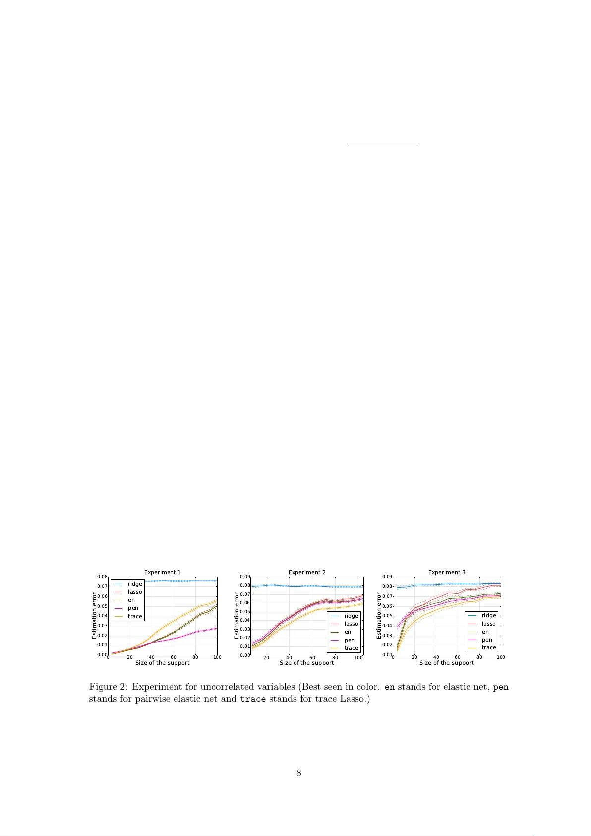
T race Lasso: a trace norm regularization for correlated designs Edouard Gra v e edouard.grave@inria.fr Guillaume Ob ozinski guillaume.obozinski@inria.fr F rancis Bac h francis.bach@inria.fr INRIA - Sierr a pr oje ct-te am L ab or atoir e d’Informatique de l’ ´ Ec ole Normale Sup´ erieur e Paris, F r anc e Abstract Using the ` 1 -norm to regularize the estimation of the parameter vector of a linear model leads to an unstable estimator when cov ariates are highly correlated. In this pap er, w e in- tro duce a new p enalt y function which tak es into accoun t the correlation of the design matrix to stabilize the estimation. This norm, called the trace Lasso, uses the trace norm, which is a con vex surrogate of the rank, of the selected cov ariates as the criterion of mo del com- plexit y . W e analyze the prop erties of our norm, describ e an optimization algorithm based on rew eighted least-squares, and illustrate the b eha vior of this norm on synthetic data, sho wing that it is more adapted to strong correlations than competing metho ds such as the elastic net. 1 In tro duction The concept of parsimony is central in many scientific domains. In the con text of statistics, signal pro cessing or machine learning, it takes the form of v ariable or feature selection problems, and is commonly used in tw o situations: first, to make the mo del or the prediction more interpretable or c heap er to use, i.e., ev en if the underlying problem does not admit sparse solutions, one looks for the b est sparse appro ximation. Second, sparsit y can also b e used given prior kno wledge that the model should b e sparse. Many metho ds ha ve been designed to learn sparse mo dels, namely metho ds based on combinatorial optimization [1, 2], Ba y esian inference [3] or conv ex optimization [4, 5]. In this pap er, w e focus on the regularization b y sparsit y-inducing norms. The simplest example of suc h norms is the ` 1 -norm, leading to the Lasso, when used within a least-squares framework. In recen t y ears, a large b o dy of work has shown that the Lasso was p erforming optimally in high- dimensional lo w-correlation settings, b oth in terms of prediction [6], estimation of parameters or estimation of supports [7, 8]. How ev er, most data exhibit strong correlations, with v arious correla- tion structures, suc h as clusters (i.e., close to blo c k-diagonal co v ariance matrices) or sparse graphs, suc h as for example problems inv olving sequences (in which case, the cov ariance matrix is close to a T o eplitz matrix [9]). In these situations, the Lasso is known to hav e stabilit y problems: although its predictive p erformance is not disastrous, the selected predictor ma y v ary a lot (typically , given t wo correlated v ariables, the Lasso will only select one of the tw o, at random). Sev eral remedies hav e been prop osed to this instability . First, the elastic net [10] adds a strongly conv ex p enalty term (the squared ` 2 -norm) that will stabilize selection (t ypically , giv en t wo correlated v ariables, the elastic net will select the tw o v ariables). Ho w ever, it is blind to the exact correlation structure, and while strong con v exity is required for some v ariables, it is not for other v ariables. Another solution is to consider the group Lasso, which will divide the predictors in to groups and p enalize the sum of the ` 2 -norm of these groups [11]. This is kno wn to accomodate strong correlations within groups [12]; ho wev er it requires to know the group in adv ance, whic h is not alw ays possible. A third line of research has focused on sampling-based techniques [13, 14, 15]. 1 An ideal regularizer should thus b e adapted to the design (lik e the group Lasso), but without requiring human in terv ention (lik e the elastic net); it should thus add strong conv exit y only where needed, and not mo difying v ariables where things b ehav e correctly . In this pap er, w e prop ose a new norm tow ards this end. More precisely we make the follo wing contributions: • W e prop ose in Section 2 a new norm based on the trace norm (a.k.a. nuclear norm) that in terp olates b et ween the ` 1 -norm and the ` 2 -norm dep ending on correlations. • W e show that there is a unique minimum when p enalizing with this norm in Section 2.2. • W e provide optimization algorithms based on rew eighted least-squares in Section 3. • W e study the second-order expansion around indep endence and relate to existing work on including correlations in Section 4. • W e p erform syn thetic exp eriments in Section 5, where w e sho w that the trace Lasso outper- forms existing norms in strong-correlation regimes. Notations. Let M ∈ R n × p . The columns of M are noted using sup erscript, i.e., M ( i ) denotes the i -th column, while the rows are noted using subscript, i.e., M i denotes the i -th row. F or M ∈ R p × p , diag( M ) ∈ R p is the diagonal of the matrix M , while for u ∈ R p , Diag( u ) ∈ R p × p is the diagonal matrix whose diagonal elements are the u i . Let S b e a subset of { 1 , ..., p } , then u S is the v ector u restricted to the supp ort S , with 0 outside the supp ort S . W e denote b y S p the set of symmetric matrices of size p . W e will use v arious matrix norms, here are the notations we use: • k M k ∗ is the trace norm, i.e. , the sum of the singular v alues of the matrix M , • k M k op is the op erator norm, i.e. , the maximum singular v alue of the matrix M , • k M k F is the F robenius norm, i.e. , the ` 2 -norm of the singular v alues, which is also equal to p tr( M > M ), • k M k 2 , 1 is the sum of the ` 2 -norm of the columns of M : k M k 2 , 1 = p X i =1 k M ( i ) k 2 . 2 Definition and prop erties of the trace Lasso W e consider the problem of predicting y ∈ R , given a v ector x ∈ R p , assuming a linear mo del y = w > x + ε, where ε is (Gaussian) noise with mean 0 and v ariance σ 2 . Given a training set X = ( x 1 , ..., x n ) > ∈ R n × p and y = ( y 1 , ..., y n ) > ∈ R n , a widely used metho d to estimate the parameter vector w is the pe- nalized empirical risk minimization ˆ w ∈ argmin w 1 n n X i =1 ` ( y i , w > x i ) + λf ( w ) , (1) where ` is a loss function used to me asure the error we make b y predicting w > x i instead of y i , while f is a regularization term used to p enalize complex mo dels. This second term helps a voiding o verfitting, especially in the case where w e ha ve man y more parameters than observ ation, i.e. , n  p . 2 2.1 Related w ork W e will now present some classical p enalty functions for linear mo dels whic h are widely used in the mac hine learning and statistics communit y . The first one, kno wn as Tikhono v regularization [16] or ridge regression [17], is the squared ` 2 -norm. When used with the square loss, estimating the parameter vector w is done by solving a linear system. One of the main drawbac ks of this p enalty function is the fact that it do es not p erform v ariable selection and thus do es not behav e well in sparse high-dimensional settings. Hence, it is natural to p enalize linear mo dels by the num b er of v ariables used by the mo del. Unfortunately , this criterion, sometimes denoted b y k · k 0 ( ` 0 -p enalt y), is not con vex and solving the problem in Eq. (1) is generally NP-hard [18]. Th us, a conv ex relaxation for this problem w as introduced, replacing the size of the selected subset b y the ` 1 -norm of w . This estimator is kno wn as the Lasso [4] in the statistics communit y and basis pursuit [5] in signal pro cessing. It w as later shown that under some assumptions, the tw o problems were in fact equiv alent (see for example [19] and references therein). When t w o predictors are highly correlated, the Lasso has a very unstable behavior: it may only select the v ariable that is the most correlated with the residual. On the other hand, the Tikhono v regularization tends to shrink co efficien ts of correlated v ariables together, leading to a v ery stable b eha vior. In order to get the b est of b oth worlds, stability and v ariable selection, Zou and Hastie introduced the elastic net [10], whic h is the sum of the ` 1 -norm and squared ` 2 -norm. Unfortunately , this estimator needs tw o regularization parameters and is not adaptiv e to the precise correlation structure of the data. Some authors also prop osed to use pairwise correlations b et w een predictors to in terp olate more adaptiv ely b etw een the ` 1 -norm and squared ` 2 -norm, by in tro ducing the pairwise elastic net [20] (see comparisons with our approach in Section 5). Finally , when one has more kno wledge ab out the data, for example clusters of v ariables that should b e selected together, one can use the group Lasso [11]. Given a partition ( S i ) of the set of v ariables, it is defined as the sum of the ` 2 -norms of the restricted vectors w S i : k w k GL = k X i =1 k w S i k 2 . The effect of this p enalt y function is to in tro duce sparsit y at the group lev el: v ariables in a group are selected altogether. One of the main drawbac k of this metho d, which is also sometimes one of its qualit y , is the fact that one needs to know the partition of the v ariables, and so one needs to ha ve a go od kno wledge of the data. 2.2 The ridge, the Lasso and the trace Lasso In this section, we show that Tikhonov regularization and the Lasso p enalty can b e view ed as norms of the matrix X Diag ( w ). W e then introduce a new norm inv olving this matrix. The solution of empirical risk minimization penalized by the ` 1 -norm or ` 2 -norm is not equiv- arian t by rescaling of the predictors X ( i ) , so it is common to normalize the predictors. When normalizing the predictors X ( i ) , and penalizing b y Tikhono v regularization or by the Lasso, peo- ple are implicitly using a regularization term that dep ends on the data or design matrix X . In fact, there is an equiv alence b et ween normalizing the predictors and not normalizing them, using the t wo follo wing reweigh ted ` 2 and ` 1 -norms instead of the Tikhonov regularization and the Lasso: k w k 2 2 = p X i =1 k X ( i ) k 2 2 w 2 i and k w k 1 = p X i =1 k X ( i ) k 2 | w i | . (2) These tw o norms can b e expressed using the matrix X Diag( w ): k w k 2 = k X Diag( w ) k F and k w k 1 = k X Diag( w ) k 2 , 1 , and a natural question arises: are there other relev ant c hoices of functions or matrix norms? A classical measure of the complexity of a model is the n um b er of predictors used by this mo del, 3 whic h is equal to the size of the supp ort of w . This p enalt y b eing non-conv ex, p eople use its con vex relaxation, which is the ` 1 -norm, leading to the Lasso. Here, we prop ose a different measure of complexit y which can b e shown to b e more adapted in mo del selection settings [21]: the dimension of the subspace spanned by the selected predictors. This is equal to the rank of the selected predictors, or also to the rank of the matrix X Diag( w ). As for the size of the supp ort, this function is non-conv ex, and w e propose to replace it by a conv ex surrogate, the tr ac e norm , leading to the follo wing p enalty that w e call “trace Lasso”: Ω( w ) = k X Diag( w ) k ∗ . The trace Lasso has some interesting prop erties: if all the predictors are orthogonal, then, it is equal to the ` 1 -norm. Indeed, w e hav e the decomp osition: X Diag( w ) = p X i =1  k X ( i ) k 2 w i  X ( i ) k X ( i ) k 2 e > i , where e i are the vectors of the canonical basis. Since the predictors are orthogonal and the e i are orthogonal to o, this gives the singular v alue decomp osition of X Diag( w ) and we get k X Diag( w ) k ∗ = p X i =1 k X ( i ) k 2 | w i | = k X Diag( w ) k 2 , 1 . On the other hand, if all the predictors are equal to X (1) , then X Diag( w ) = X (1) w > , and we get k X Diag( w ) k ∗ = k X (1) k 2 k w k 2 = k X Diag( w ) k F , which is equiv alent to the Tikhonov regularization. Th us when tw o predictors are strongly correlated, our norm will b ehav e like the Tikhono v regularization, while for almost uncorrelated predictors, it will b eha v e like the Lasso. Alw ays ha ving a unique minimum is an imp ortant property for a statistical estimator, as it is a first step tow ards stability . The trace Lasso, b y adding strong conv exit y exactly in the direction of highly correlated co v ariates, alwa ys has a unique minim um, and is m uch more stable than the Lasso. Prop osition 1. If the loss function ` is str ongly c onvex with r esp e ct to its se c ond ar gument, then the solution of the empiric al risk minimization p enalize d by the tr ac e L asso, i.e., Eq. (1), is unique. The tec hnical pro of of this prop osition is given in app endix B, and consists of showing that in the flat directions of the loss function, the trace Lasso is strongly con v ex. 2.3 A new family of p enalt y functions In this section, w e introduce a new family of p enalties, inspired by the trace Lasso, allowing us to write the ` 1 -norm, the ` 2 -norm and the newly introduced trace Lasso as sp ecial cases. In fact, w e note that k Diag ( w ) k ∗ = k w k 1 and k p − 1 / 2 1 > Diag( w ) k ∗ = k w > k ∗ = k w k 2 . In other words, w e can express the ` 1 and ` 2 -norms of w using the trace norm of a giv en matrix times the matrix Diag( w ). A natural question to ask is: what happ ens when using a matrix P other than the iden tity or the line vector p − 1 / 2 1 > , and what are go o d choices of suc h matrices? Therefore, we in tro duce the following family of penalty functions: Definition 1. L et P ∈ R k × p , al l of its c olumns having unit norm. We intr o duc e the norm Ω P as Ω P ( w ) = k P Diag( w ) k ∗ . Pr o of. The p ositiv e homogeneity and triangle inequality are direct consequences of the linearit y of w 7→ P Diag ( w ) and the fact that k · k ∗ is a norm. Since all the columns of P are not equal to zero, we ha ve P Diag( w ) = 0 ⇔ w = 0 , and so, Ω P separates p oin ts and is a norm. 4 Figure 1: Unit balls for v arious v alue of P > P . See the text for the v alue of P > P . (Best seen in color). As stated b efore, the ` 1 and ` 2 -norms are sp ecial cases of the family of norms w e just introduced. Another imp ortant p enalt y that can b e expressed as a sp ecial case is the group Lasso, with non- o verlapping groups. Given a partition ( S j ) of the set { 1 , ..., p } , the group Lasso is defined b y k w k GL = X S j k w S j k 2 . W e define the matrix P GL b y P GL ij =  1 / p | S k | if i and j are in the same group S k , 0 otherwise. Then, P GL Diag( w ) = X S j 1 S j p | S j | w > S j . (3) Using the fact that ( S j ) is a partition of { 1 , ..., p } , the vectors 1 S j are orthogonal and so are the v ectors w S j . Hence, after normalizing the v ectors, Eq. (3) gives a singular v alue decomp osition of P GL Diag( w ) and so the group Lasso penalty can b e expressed as a sp ecial case of our family of norms: k P GL Diag( w ) k ∗ = X S j k w S j k 2 = k w k GL . In the following prop osition, we sho w that our norm only depends on the v alue of P > P . This is an imp ortan t prop erty for the trace Lasso, where P = X , since it underlies the fact that this p enalt y only dep ends on the correlation matrix X > X of the co v ariates. Prop osition 2. L et P ∈ R k × p , al l of its c olumns having unit norm. We have Ω P ( w ) = k ( P > P ) 1 / 2 Diag( w ) k ∗ . W e plot the unit ball of our norm for the following v alue of P > P (see figure (1)):   1 0 . 9 0 . 1 0 . 9 1 0 . 1 0 . 1 0 . 1 1     1 0 . 7 0 . 49 0 . 7 1 0 . 7 0 . 49 0 . 7 1     1 1 0 1 1 0 0 0 1   W e can low er b ound and upp er b ound our norms b y the ` 2 -norm and ` 1 -norm resp ectively . This shows that, as for the elastic net, our norms interpolate betw een the ` 1 -norm and the ` 2 - norm. But the main difference betw een the elastic net and our norms is the fact that our norms are adaptive , and require a single regularization parameter to tune. In particular for the trace 5 Lasso, when t w o cov ariates are strongly correlated, it will be close to the ` 2 -norm, while when tw o co v ariates are almost uncorrelated, it will b eha v e lik e the ` 1 -norm. This is a b ehavior close to the one of the pairwise elastic net [20]. Prop osition 3. L et P ∈ R k × p , al l of its c olumns having unit norm. We have k w k 2 ≤ Ω P ( w ) ≤ k w k 1 . 2.4 Dual norm The dual norm is an imp ortant quan tity for b oth optimization and theoretical analysis of the estimator. Unfortunately , w e are not able in general to obtain a closed form expression of the dual norm for the family of norms we just introduced. How ever we can obtain a b ound, whic h is exact for some sp ecial cases: Prop osition 4. The dual norm, define d by Ω ∗ P ( u ) = max Ω P ( v ) ≤ 1 u > v , c an b e b ounde d by: Ω ∗ P ( u ) ≤ k P Diag( u ) k op . Pr o of. Using the fact that diag ( P > P ) = 1 , we ha ve u > v = tr  Diag( u ) P > P Diag( v )  ≤ k P Diag( u ) k op k P Diag( v ) k ∗ , where the inequality comes from the fact that the op erator norm k · k op is the dual norm of the trace norm. The definition of the dual norm then gives the result. As a corollary , we can b ound the dual norm by a constant times the ` ∞ -norm: Ω ∗ P ( u ) ≤ k P Diag( u ) k op ≤ k P k op k Diag( u ) k op = k P k op k u k ∞ . Using prop osition (3), we also hav e the inequality Ω ∗ P ( u ) ≥ k u k ∞ . 3 Optimization algorithm In this section, w e in tro duce an algorithm to estimate the parameter vector w when the loss function is equal to the square loss: ` ( y , w > x ) = 1 2 ( y − w > x ) 2 and the p enalty is the trace Lasso. It is straightforw ard to extend this algorithm to the family of norms indexed by P . The problem w e consider is min w 1 2 k y − Xw k 2 2 + λ k X Diag( w ) k ∗ . W e could optimize this cost function by subgradien t descent, but this is quite inefficient: computing the subgradient of the trace Lasso is exp ensiv e and the rate of conv ergence of subgradien t descen t is quite slow. Instead, w e consider an iteratively rew eighted least-squares metho d. First, we need to introduce a w ell-known v ariational formulation for the trace norm [22]: Prop osition 5. L et M ∈ R n × p . The tr ac e norm of M is e qual to: k M k ∗ = 1 2 inf S  0 tr  M > S − 1 M  + tr ( S ) , and the infimum is attaine d for S =  MM >  1 / 2 . 6 Using this prop osition, we can reformulate the previous optimization problem as min w inf S  0 1 2 k y − Xw k 2 2 + λ 2 w > Diag  diag( X > S − 1 X )  w + λ 2 tr( S ) . This problem is jointly con v ex in ( w , S ) [23]. In order to optimize this ob jectiv e function by alternating the minimization o ver w and S , w e need to add a term λµ i 2 tr( S − 1 ). Otherwise, the infim um ov er S could b e attained at a non inv ertible S , leading to a non conv ergent algorithm. The infimum o ver S is then attained for S =  X Diag( w ) 2 X > + µ i I  1 / 2 . Optimizing ov er w is a least-squares problem p enalized b y a reweigh ted ` 2 -norm equal to w > Dw , where D = Diag  diag( X > S − 1 X )  . It is equiv alent to solving the linear system ( X > X + λ D ) w = X > y . This can b e done efficiently by using a conjugate gradient metho d. Since the cost of multiplying ( X > X + λ D ) by a v ector is O ( np ), solving the system has a complexit y of O ( knp ), where k ≤ p is the n um b er of iterations needed to conv erge. Using warm restarts, k can b e muc h smaller than p , since the linear system w e are solving do es not change a lot from an iteration to another. Below w e summarize the algorithm: Itera tive algorithm for estima ting w Input: the design matrix X , the initial guess w 0 , num b er of iteration N , sequence µ i . F or i = 1 ...N : • Compute the eigen v alue decomposition U Diag( s k ) U > of X Diag ( w i − 1 ) 2 X > . • Set D = Diag (diag( X > S − 1 X )), where S − 1 = U Diag(1 / √ s k + µ i ) U > . • Set w i b y solving the system ( X > X + λ D ) w = X > y . F or the sequence µ i , we use a decreasing sequence con verging to ten times the machine precision. 3.1 Choice of λ W e no w giv e a metho d to choose the regularization path. In fact, w e kno w that the vector 0 is solution if and only if λ ≥ Ω ∗ ( X > y ) [24]. Thus, w e need to start the path at λ = Ω ∗ ( X > y ), corresp onding to the empty solution 0 , and then decrease λ . Using the inequalities on the dual norm we obtained in the previous section, we get k X > y k ∞ ≤ Ω ∗ ( X > y ) ≤ k X k op k X > y k ∞ . Therefore, starting the path at λ = k X k op k X > y k ∞ is a go o d choice. 4 Appro ximation around the Lasso In this section, w e compute the second order approximation of our norm around the special case corresp onding to the Lasso. W e recall that when P = I ∈ R p × p , our norm is equal to the ` 1 -norm. W e add a small p erturbation ∆ ∈ S p to the identit y matrix, and using Prop. 6 of the app endix A, w e obtain the following second order approximation: k ( I + ∆) Diag( w ) k ∗ = k w k 1 + diag(∆) > | w | + X | w i | > 0 X | w j | > 0 (∆ j i | w i | − ∆ ij | w j | ) 2 4( | w i | + | w j | ) + X | w i | =0 X | w j | > 0 (∆ ij | w j | ) 2 2 | w j | + o ( k ∆ k 2 ) . 7 W e can rewrite this appro ximation as k ( I + ∆) Diag( w ) k ∗ = k w k 1 + diag(∆) > | w | + X i,j ∆ 2 ij ( | w i | − | w j | ) 2 4( | w i | + | w j | ) + o ( k ∆ k 2 ) , using a slight abuse of notation, considering that the last term is equal to 0 when w i = w j = 0. The second order term is quite interesting: it shows that when tw o cov ariates are correlated, the effect of the trace Lasso is to shrink the corresponding coefficients tow ard each other. Another in teresting remark is the fact that this term is very similar to pairwise elastic net p enalties, which are of the form | w | > P | w | , where P ij is a decreasing function of ∆ ij . 5 Exp erimen ts In this section, w e p erform synthetic exp erimen ts to illustrate the b eha vior of the trace Lasso and other classical p enalties when there are highly correlated cov ariates in the design matrix. F or all exp erimen ts, w e hav e p = 1024 cov ariates and n = 256 observ ations. The supp ort S of w is equal to { 1 , ..., k } , where k is the size of the supp ort. F or i in the supp ort of w , we hav e w i = 2 ( b i − 1 / 2), where each b i is indep endently drawn from a uniform distribution on [0 , 1]. The observ ations x i are drawn from a m ultiv ariate Gaussian with mean 0 and cov ariance matrix Σ. F or the first exp erimen t, Σ is set to the identit y , for the second exp eriment, Σ is blo ck diagonal with blo cks equal to 0 . 2 I + 0 . 8 11 > corresp onding to clusters of eigh t v ariables, finally for the third exp eriment, we set Σ ij = 0 . 95 | i − j | , corresp onding to a T oeplitz design. F or each metho d, we c ho ose the b est λ for the estimation error, which is rep orted. Ov erall all metho ds b ehav e similarly in the noiseless and the noisy settings, hence we only rep ort results for the noisy setting. In all three graphs of Figure 2, we observe b eha viors that are typical of Lasso, ridge and elastic net: the Lasso p erforms very w ell on sparse mo dels, but its p erformance is rather po or for denser mo dels, almost as p o or as the ridge regression. The elastic net offers the best of both w orlds since its tw o parameters allow it to in terp olate adaptively b etw een the Lasso and the ridge. In exp erimen t 1, since the v ariables are uncorrelated, there is no reason to couple their selection. This s uggests that the Lasso should b e the most appropriate conv ex regularization. The trace Lasso approaches the Lasso as n go es to infinit y , but the w eak coupling induced b y empirical correlations is sufficien t to slightly decrease its performance compared to that of the Lasso. By con trast, in exp erimen ts 2 and 3, the trace Lasso outp erforms other metho ds (including the pairwise elastic net) since v ariables that should b e selected together are indeed correlated. As for the p enalized elastic net, since it takes in to account the correlations b etw een v ariables it is not surprising that in exp eriment 2 and 3 it p erforms b etter than methods that do not. W e do not ha ve a comp elling explanation for its sup erior p erformance in exp eriment 1. 0 20 40 60 80 100 Size of the support 0.00 0.01 0.02 0.03 0.04 0.05 0.06 0.07 0.08 Estimation error Experiment 1 ridge lasso en pen trace 20 40 60 80 100 Size of the support 0.00 0.01 0.02 0.03 0.04 0.05 0.06 0.07 0.08 0.09 Estimation error Experiment 2 ridge lasso en pen trace 0 20 40 60 80 100 Size of the support 0.01 0.02 0.03 0.04 0.05 0.06 0.07 0.08 0.09 Estimation error Experiment 3 ridge lasso en pen trace Figure 2: Exp erimen t for uncorrelated v ariables (Best seen in color. en stands for elastic net, pen stands for pairwise elastic net and trace stands for trace Lasso.) 8 6 Conclusion W e introduce a new p enalty function, the trace Lasso, whic h takes adv an tage of the correlation b et w een cov ariates to add strong con v exity exactly in the directions where needed, unlike the elastic net for example, whic h blindly adds a squared ` 2 -norm term in every directions. W e sho w on synthetic data that this adaptiv e behavior leads to b etter estimation p erformance. In the future, we w ant to show that if a dedicated norm using prior knowledge such as the group Lasso can b e used, the trace Lasso will b eha ve similarly and its p erformance will not degrade to o m uch, pro viding theoretical guarantees to such adaptivity . Finally , we will seek applications of this estimator in inv erse problems suc h as deblurring, where the design matrix exhibits strong correlation structure. Ac knowledgemen ts This pap er was partially supp orted by the Europ ean Research Council (SIERRA Pro ject ERC- 239993). References [1] S.G. Mallat and Z. Zhang. Matc hing pursuits with time-frequency dictionaries. Signal Pr o- c essing, IEEE T r ansactions on , 41(12):3397–3415, 1993. [2] T. Zhang. Adaptive forward-bac kward greedy algorithm for sparse learning with linear mod- els. A dvanc es in Neur al Information Pr o c essing Systems , 22, 2008. [3] M.W. Seeger. Bay esian inference and optimal design for the sparse linear mo del. The Journal of Machine L e arning R ese ar ch , 9:759–813, 2008. [4] R. Tibshirani. Regression shrink age and selection via the Lasso. Journal of the R oyal Statis- tic al So ciety. Series B (Metho dolo gic al) , 58(1):267–288, 1996. [5] S.S. Chen, D.L. Donoho, and M.A. Saunders. Atomic decomp osition b y basis pursuit. SIAM journal on scientific c omputing , 20(1):33–61, 1999. [6] P .J. Bic kel, Y. Rito v, and A.B. Tsybako v. Simultaneous analysis of Lasso and Dantzig selector. The A nnals of Statistics , 37(4):1705–1732, 2009. [7] P . Zhao and B. Y u. On model selection consistency of Lasso. The Journal of Machine L e arning R ese ar ch , 7:2541–2563, 2006. [8] M.J. W ainwrigh t. Sharp thresholds for high-dimensional and noisy sparsity recov ery using ` 1 -constrained quadratic programming (Lasso). Information The ory, IEEE T r ansactions on , 55(5):2183–2202, 2009. [9] G.H. Golub and C.F. V an Loan. Matrix c omputations . Johns Hopkins Univ Pr, 1996. [10] H. Zou and T. Hastie. Regularization and v ariable selection via the elastic net. Journal of the R oyal Statistic al So ciety: Series B (Statistic al Metho dolo gy) , 67(2):301–320, 2005. [11] M. Y uan and Y. Lin. Mo del selection and estimation in regression with group ed v ariables. Journal of the R oyal Statistic al So ciety: Series B (Statistic al Metho dolo gy) , 68(1):49–67, 2006. [12] F.R. Bach. Consistency of the group Lasso and multiple k ernel learning. The Journal of Machine L e arning R ese ar ch , 9:1179–1225, 2008. [13] F.R. Bach. Bolasso: model consistent Lasso estimation through the bo otstrap. In Pr o c e e dings of the 25th international c onfer enc e on Machine le arning , pages 33–40. A CM, 2008. 9 [14] H. Liu, K. Ro eder, and L. W asserman. Stability approach to regularization selection (stars) for high dimensional graphical mo dels. A dvanc es in Neur al Information Pr o c essing Systems , 23, 2010. [15] N. Meinshausen and P . B ¨ uhlmann. Stability selection. Journal of the R oyal Statistic al So ciety: Series B (Statistic al Metho dolo gy) , 72(4):417–473, 2010. [16] A. Tikhonov. Solution of incorrectly formulated problems and the regularization metho d. In Soviet Math. Dokl. , volume 5, page 1035, 1963. [17] A.E. Ho erl and R.W. Kennard. Ridge regression: Biased estimation for nonorthogonal prob- lems. T e chnometrics , 12(1):55–67, 1970. [18] G. Da vis, S. Mallat, and M. Av ellaneda. Adaptiv e greedy appro ximations. Constructive appr oximation , 13(1):57–98, 1997. [19] E.J. Candes and T. T ao. Decoding by linear programming. Information The ory, IEEE T r ansactions on , 51(12):4203–4215, 2005. [20] A. Lorbert, D. Eis, V. Kostina, D. M. Blei, and P . J. Ramadge. Exploiting co v ariate similarit y in sparse regression via the pairwise elastic net. JMLR - Pr o c e e dings of the 13th International Confer enc e on Artificial Intel ligenc e and Statistics , 9:477–484, 2010. [21] T. Hastie, R. Tibshirani, and J. F riedman. The elements of statistical learning. 2001. [22] A. Argyriou, T. Evgeniou, and M. P on til. Multi-task feature learning. A dvanc es in neur al information pr o c essing systems , 19:41, 2007. [23] S.P . Boyd and L. V anden b erghe. Convex optimization . Cambridge Univ Pr, 2004. [24] F. Bach, R. Jenatton, J. Mairal, and G. Ob ozinski. Conv ex optimization with sparsity- inducing norms. S. Sr a, S. Nowozin, S. J. Wright., e ditors, Optimization for Machine L e arn- ing , 2011. [25] F.R. Bach. Consistency of trace norm minimization. The Journal of Machine L e arning R ese ar ch , 9:1019–1048, 2008. 10 A P erturbation of the trace norm W e follo w the tec hnique used in [25] to obtain an approximation of the trace norm. A.1 Jordan-Wielandt matrices Let M ∈ R n × p of rank r . W e note s 1 ≥ s 2 ≥ ... ≥ s r > 0, the strictly p ositive singular v alues of M and u i , v i the asso ciated left and righ t singular vectors. W e introduce the Jordan-Wielandt matrix ˜ M =  0 M M > 0  ∈ R ( n + p ) × ( n + p ) . The singular v alues of M and the eigen v alues of ˜ M are related: ˜ M has eigen v alues s i and s − i = − s i asso ciated to eigenv ectors w i = 1 √ 2  u i v i  and w − i = 1 √ 2  u i − v i  . The remaining eigenv alues of ˜ M are equal to 0 and are asso ciated to eigenv ectors of the form w = 1 √ 2  u v  and w = 1 √ 2  u − v  , where ∀ i ∈ { 1 , ..., r } , u > u i = v > v i = 0. A.2 Cauc h y residue form ula Let C b e a closed curv e that do es not go through the eigenv alues of ˜ M . W e define Π C ( ˜ M ) = 1 2 iπ Z C λ ( λ I − ˜ M ) − 1 dλ. W e ha v e Π C ( ˜ M ) = 1 2 iπ I X j λ λ − s j w j w > j dλ = 1 2 iπ I X j  1 + s j λ − s j  w j w > j dλ = X s j ∈C s j w j w > j . A.3 P erturbation analysis Let ∆ ∈ R n × p b e a perturbation matrix suc h that k ∆ k op < s r / 4, and let C b e a closed curv e around the r largest eigen v alues of ˜ M and ˜ M + ˜ ∆ . W e can study the perturbation of the strictly p ositiv e singular v alues of M b y computing the trace of Π C ( ˜ M + ˜ ∆ ) − Π C ( ˜ M ). Using the fact that ( λ I − ˜ M − ˜ ∆ ) − 1 = ( λ I − ˜ M ) − 1 + ( λ I − ˜ M ) − 1 ˜ ∆ ( λ I − ˜ M − ˜ ∆ ) − 1 , we ha ve Π C ( ˜ M + ˜ ∆ ) − Π C ( ˜ M ) = 1 2 iπ I λ ( λ I − ˜ M ) − 1 ˜ ∆ ( λ I − ˜ M ) − 1 dλ + 1 2 iπ I λ ( λ I − ˜ M ) − 1 ˜ ∆ ( λ I − ˜ M ) − 1 ˜ ∆ ( λ I − ˜ M ) − 1 dλ + 1 2 iπ I λ ( λ I − ˜ M ) − 1 ˜ ∆ ( λ I − ˜ M ) − 1 ˜ ∆ ( λ I − ˜ M − ˜ ∆ ) − 1 dλ. 11 W e note A and B the first tw o terms of the right hand side of this equation. W e ha ve tr( A ) = X j,k tr( w j w > j ˜ ∆w k w > k ) 1 2 iπ I C λdλ ( λ − s j )( λ − s k ) = X j tr( w > j ˜ ∆w j ) 1 2 iπ I C λdλ ( λ − s j ) 2 = X j tr( w > j ˜ ∆w j ) = X j tr( u > j ∆v j ) , and tr( B ) = X j,k,l tr( w j w > j ˜ ∆w k w > k ˜ ∆w l w > l ) 1 2 iπ I C λdλ ( λ − s j )( λ − s k )( λ − s l ) = X j,k tr( w j ˜ ∆w k w k ˜ ∆w j ) 1 2 iπ I C λdλ ( λ − s j ) 2 ( λ − s k ) . If s j = s k , the integral is nul. Otherwise, we ha ve λ ( λ − s j ) 2 ( λ − s k ) = a λ − s j + b λ − s k + c ( λ − s j ) 2 , where a = − s k ( s k − s j ) 2 , b = s k ( s k − s j ) 2 , c = s j s j − s k . Therefore, if s j and s k are b oth inside or outside the interior of C , the integral is equal to zero. So tr( B ) = X s j > 0 X s k ≤ 0 − s k ( w > j ˜ ∆w k ) 2 ( s j − s k ) 2 + X s j ≤ 0 X s k > 0 s k ( w > j ˜ ∆w k ) 2 ( s j − s k ) 2 = X s j > 0 X s k > 0 s k ( w > j ˜ ∆w − k ) 2 ( s j + s k ) 2 + X s j > 0 X s k > 0 s k ( w > − j ˜ ∆w k ) 2 ( s j + s k ) 2 + X s j =0 X s k > 0 ( w > j ˜ ∆w k ) 2 s k = X s j > 0 X s k > 0 ( w > − j ˜ ∆w k ) 2 s j + s k + X s j =0 X s k > 0 ( w > j ˜ ∆w k ) 2 s k . F or s j > 0 and s k > 0, w e hav e w > − j ˜ ∆w k = 1 2  u > j ∆v k − u > k ∆v j  , and for s j = 0 and s k > 0, w e hav e w > j ˜ ∆w k = 1 2  ± u > k ∆v j + u > j ∆v k  . So tr( B ) = X s j > 0 X s k > 0 ( u > j ∆v k − u > k ∆v j ) 2 4( s j + s k ) + X s j =0 X s k > 0 ( u > k ∆v j ) 2 + ( u > j ∆v k ) 2 2 s k . 12 No w, let C 0 b e the circle of center 0 and radius s r / 2. W e can study the p erturbation of the singular v alues of M equal to zero by computing the trace norm of Π C 0 ( ˜ M + ˜ ∆ ) − Π C 0 ( ˜ M ). W e ha ve Π C 0 ( ˜ M + ˜ ∆ ) − Π C 0 ( ˜ M ) = 1 2 iπ I C 0 λ ( λ I − ˜ M ) − 1 ˜ ∆ ( λ I − ˜ M ) − 1 dλ + 1 2 iπ I C 0 λ ( λ I − ˜ M ) − 1 ˜ ∆ ( λ I − ˜ M ) − 1 ˜ ∆ ( λ I − ˜ M ) − 1 dλ + 1 2 iπ I C 0 λ ( λ I − ˜ M ) − 1 ˜ ∆ ( λ I − ˜ M ) − 1 ˜ ∆ ( λ I − ˜ M − ˜ ∆ ) − 1 dλ. Then, if we note the first integral C and the second one D , we get C = X j,k w j w > j ˜ ∆w k w > k 1 2 iπ I C 0 λdλ ( λ − s j )( λ − s k ) . If b oth s j and s k are outside int ( C 0 ), then the in tegral is equal to zero. If one of them is inside, sa y s j , then s j = 0 and the in tegral is equal to I C 0 dλ λ − s k Then this integral is non n ul if and only if s k is also inside int ( C 0 ). Thus C = X j,k w j w > j ˜ ∆w k w > k 1 s j ∈ int ( C 0 ) 1 s k ∈ int ( C 0 ) = X s j =0 X s k =0 w j w > j ˜ ∆w k w > k = W 0 W > 0 ˜ ∆W 0 W > 0 , where W 0 are the eigenv ectors asso ciated to the eigenv alue 0. W e hav e D = X j,k,l w j w > j ˜ ∆w k w > k ˜ ∆w l w > l 1 2 iπ I C 0 λdλ ( λ − s j )( λ − s k )( λ − s l ) . The integral is not equal to zero if and only if exactly one eigenv alue, say s i , is outside int ( C 0 ). The integral is then equal to − 1 /s i . Thus D = − W 0 W > 0 ˜ ∆W 0 W > 0 ˜ ∆W S − 1 W > − W S − 1 W > ˜ ∆W 0 W > 0 ˜ ∆W 0 W > 0 − W 0 W > 0 ˜ ∆W S − 1 W > ˜ ∆W 0 W > 0 , where S = Diag ( − s , s ). Finally , putting everything together, we get Prop osition 6. L et M = U Diag( s ) V > ∈ R n × p , the singular value de c omp osition of M , with U ∈ R n × r , V ∈ R p × r . L et ∆ ∈ R n × p . We have k M + ∆ k ∗ = k M k ∗ + k Q k ∗ + tr( VU > ∆ )+ X s j > 0 X s k > 0 ( u > j ∆v k − u > k ∆v j ) 2 4( s j + s k ) + X s j =0 X s k > 0 ( u > k ∆v 0 j ) 2 + ( u > 0 j ∆v k ) 2 2 s k + o ( k ∆ k 2 ) , wher e Q = U > 0 ∆ V 0 − U > 0 ∆ V 0 V > 0 ∆ > U Diag( s ) − 1 − Diag( s ) − 1 V > ∆ > U 0 U > 0 ∆ V 0 − U > 0 ∆ V Diag( s ) − 1 U > ∆ V 0 . 13 B Pro of of prop osition 1 In this section, we prov e that if the loss function is strongly conv ex with resp ect to its second argumen t, then the solution of the p enalized empirical risk minimization is unique. Let ˆ w ∈ argmin w P n i =1 ` ( y i , w > x i ) + λ k X Diag( w ) k ∗ . If ˆ w is in the n ullspace of X , then ˆ w = 0 and the minimum is unique. F rom now on, w e supp ose that the minima are not in the nullspace of X . Let u , v ∈ argmin w P n i =1 ` ( y i , w > x i ) + λ k X Diag ( w ) k ∗ and δ = v − u . By con vexit y of the ob jective function, all the w = u + tδ , for t ∈ ]0 , 1[ are also optimal solutions, and so, w e can choose an optimal solution w suc h that w i 6 = 0 for all i in the supp ort of δ . Because the loss function is strongly conv ex outside the nullspace of X , δ is in the nullspace of X . Let X Diag( w ) = U Diag( s ) V > b e the SVD of X Diag( w ). W e hav e the follo wing dev elopment around w : k X Diag( w + tδ ) k ∗ = k X Diag( w ) k ∗ + tr(Diag( tδ ) X > UV > )+ X s i > 0 X s j > 0 tr(Diag( tδ ) X > ( u i v > j − u j v > i )) 2 4( s i + s j ) + X s i > 0 X s j =0 tr(Diag( tδ ) X > u i v > j ) 2 2 s i + o ( t 2 ) . W e note S the supp ort of w . Using the fact that the supp ort of δ is included in S , w e hav e X Diag( tδ ) = X Diag( w ) Diag( tγ ), where γ i = δ i w i for i ∈ S and 0 otherwise. Then: k X Diag( w + tδ ) k ∗ = k X Diag( w ) k ∗ + tγ > diag( V Diag( s ) V > )+ X s i > 0 X s j > 0 t 2 tr  ( s i − s j ) Diag( γ ) v i v > j  2 4( s i + s j ) + X s i > 0 X s j =0 t 2 tr  s i Diag( γ ) v i v > j  2 2 s i + o ( t 2 ) . F or small t , w + tδ is also a minimum, and therefore, we ha ve: ∀ s i > 0 , s j > 0 , ( s i − s j ) tr  Diag( γ ) v i v > j  = 0 , (4) ∀ s i > 0 , s j = 0 , tr  Diag( γ ) v i v > j  = 0 . (5) This could b e summarized as ∀ s i 6 = s j , v > i (Diag( γ ) v j ) = 0 . (6) This means that the eigenspaces of Diag( w ) X > X Diag( w ) are stable by the matrix Diag ( γ ). Therefore, Diag( w ) X > X Diag( w ) and Diag ( γ ) are sim ultaneously diagonalizable and so, they comm ute. Therefore: ∀ i, j ∈ S, σ ij γ i = σ ij γ j (7) where σ ij = [ X > X ] ij . W e define a partition ( S k ) of S , suc h that i and j are in the same set S k if there exists a path i = a 1 , ..., a m = j such that σ a n ,a n +1 6 = 0 for all n ∈ { 1 , ..., m − 1 } . Then, using equation (7), γ is constan t on eac h S k . δ b eing in the n ullspace of X , w e hav e: 0 = δ > X > X δ (8) = X S k X S l δ > S k X > X δ S l (9) = X S k δ > S k X > X δ S k (10) = X S k k X δ S k k 2 2 . (11) 14 So for all S i , X δ S i = 0. Since a predictor X i is orthogonal to all the predictors b elonging to other groups defined by the partition ( S k ), we can decomp ose the norm Ω: k X Diag( w ) k ∗ = X S k k X Diag( w S k ) k ∗ . (12) W e recall that γ is constant on each S k and so δ S k is colinear to w S i , by definition of γ . If δ S i is not equal to zero, this means that w S i , whic h is not equal to zero, is in the n ullspace of X . Replacing w S i b y 0 will not change the v alue of the data fitting term but it will strictly decreases the v alue of the norm Ω. This is a con tradiction with the optimality of w . Thus all the δ S i are equal to zero and the minimum is unique. C Pro of of prop osition 3 F or the first inequality , w e hav e k w k 2 = k P Diag( w ) k F ≤ k P Diag( w ) k ∗ . F or the second inequality , w e hav e k P Diag( w ) k ∗ = max k M k op ≤ 1 tr  M > P Diag( w )  = max k M k op ≤ 1 diag  M > P  > w ≤ max k M k op ≤ 1 p X i =1 | M ( i ) > P ( i ) | | w i | ≤ k w k 1 . The first equalit y is the fact that the dual norm of the trace norm is the op erator norm and the second inequality uses the fact that all matrices of op erator norm smaller than one ha v e columns of ` 2 norm smaller than one. 15