Modern hierarchical, agglomerative clustering algorithms

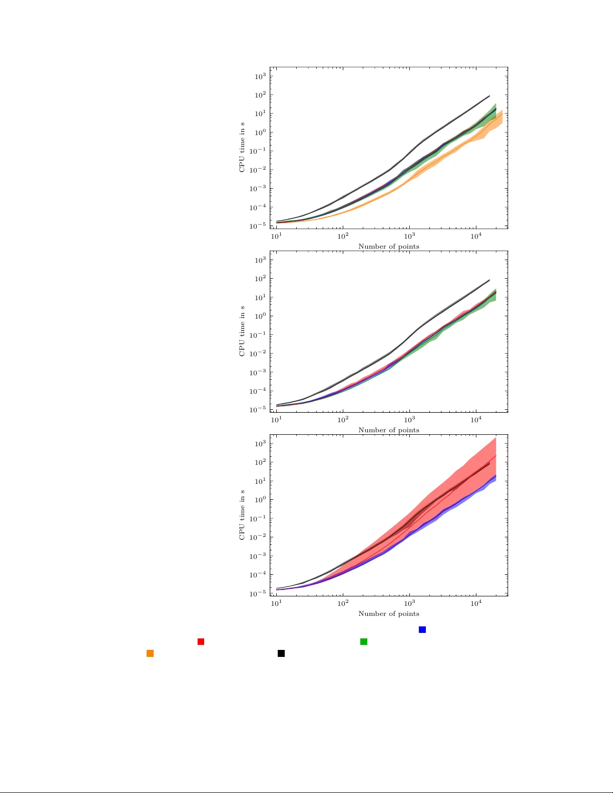
Mo dern hierarc hical, agglomerativ e clustering algorithms D aniel Müllner This pap er presen ts algorithms for hierarc hical, agglomerativ e clustering which p erform most eﬃcien tly in the general-purpose setup that is giv en in mo dern standard soft w are. Requiremen ts are: (1) the input data is giv en by pairwise dis- similarities b etw een data p oin ts, but extensions to vector data are also discussed (2) the output is a “step wise dendrogram”, a data structure which is shared by all implemen tations in curren t standard soft w are. W e presen t algorithms (old and new) whic h perform clustering in this setting eﬃciently , b oth in an asymptotic w orst-case analysis and from a practical p oint of view. The main contributions of this paper are: (1) W e present a new algorithm which is suitable for any distance up date scheme and performs signiﬁcantly b etter than the existing algorithms. (2) W e prov e the correctness of tw o algorithms by Rohlf and Murtagh, which is neces- sary in eac h case for diﬀeren t reasons. (3) W e giv e w ell-founded recommendations for the b est current algorithms for the v arious agglomerative clustering sc hemes. Keyw ords: clustering, hierarchical, agglomerativ e, partition, linkage 1 In tro duction Hierarc hical, agglomerative clustering is an imp ortant and w ell-established technique in un- sup ervised machine learning. Agglomerativ e clustering sc hemes start from the partition of the data set in to singleton no des and merge step by step the current pair of mutually closest no des into a new no de until there is one ﬁnal no de left, which comprises the entire data set. V arious clustering sc hemes share this pro cedure as a common deﬁnition, but diﬀer in the w a y in which the measure of in ter-cluster dissimilarit y is up dated after each step. The seven most common metho ds are termed single, complete, av erage (UPGMA), weigh ted (WPGMA, Mc- Quitt y), W ard, cen troid (UPGMC) and median (WPGMC) linkage (see Everitt et al., 2011, T able 4.1). They are implemen ted in standard numerical and statistical softw are suc h as R (R Developmen t Core T eam, 2011), MA TLAB (The Math W orks, Inc., 2011), Mathematica (W olfram Researc h, Inc., 2010), SciPy (Jones et al., 2001). The stepwise, pro cedural deﬁnition of these clustering methods directly gives a v alid but ineﬃcien t clustering algorithm. Starting with Go wer’s and Ross’s observ ation (Gow er and Ross, 1969) that single linkage clustering is related to the minim um spanning tree of a graph in 1969, sev eral authors ha v e contributed algorithms to reduce the computational complexit y of agglomerative clustering, in particular Sibson (1973), Rohlf (1973), Anderb erg (1973, page 135), Murtagh (1984), Day and Edelsbrunner (1984, T able 5). 1 Ev en when soft w are pac kages do not use the ineﬃcien t primitive algorithm (as SciPy (Eads, 2007) and the R (R Dev elopment Core T eam, 2011) metho ds hclust and agnes do), the author found that implemen tations largely use sub optimal algorithms rather than impro v ed metho ds suggested in theoretical work. This paper is to adv ance the theory further up to a p oin t where the algorithms can be readily used in the standard setting, and in this w a y bridge the gap betw een the theoretical adv ances that ha ve b een made and the existing soft w are implemen tations, which are widely used in science and industry . The main contributions of this pap er are: • W e presen t a new algorithm which is suitable for an y distance update sc heme and p er- forms signiﬁcan tly b etter than the existing algorithms for the “centroid” and “median” clustering schemes. • W e pro v e the correctness of tw o algorithms, a single linkage algorithm by Rohlf (1973) and Murtagh’s nearest-neighbor-chain algorithm (Murtagh, 1985, page 86). These pro ofs w ere still missing, and w e detail wh y the t w o proofs are necessary , each for diﬀeren t reasons. • These three algorithms (together with an alternativ e by Sibson, 1973) are the best curren tly av ailable ones, each for its o wn subset of agglomerativ e clustering schemes. W e justify this carefully , discussing p otential alternativ es. The sp eciﬁc class of clustering algorithms whic h is dealt with in this pap er has been c har- acterized by the acron ym SAHN (sequential, agglomerative, hierarchic, nonov erlapping meth- o ds) b y Sneath and Sokal (1973, § 5.4, 5.5). The procedural deﬁnition (whic h is giv en in Figure 1 b elow) is not the only p ossibility for a SAHN metho d, but this metho d together with the seven common distance up date sc hemes listed ab ov e is most widely used. The scope of this pap er is contained further b y practical considerations: W e consider metho ds here whic h comply to the input and output requirements of the general-purp ose clustering functions in mo dern standard softw are: • The input to the algorithm is the list of  N 2  pairwise dissimilarities b etw een N points. (W e men tion extensions to v ector data in Section 6.) • The output is a so called stepwise dendr o gr am (see Section 2.2), in contrast to laxly sp eciﬁed output structure or weak er notions of (non-stepwise) dendrograms in earlier literature. The ﬁrst item has alwa ys b een a distinctive c haracteristic to previous authors since the input format broadly divides into the stor e d matrix appr o ach (Anderb erg, 1973, § 6.2) and the stor e d data appr o ach (Anderb erg, 1973, § 6.3). In contrast, the second condition has not b een given atten tion yet, but we will see that it aﬀects the v alidit y of algorithms. W e do not aim to present and compare all av ailable clustering algorithms but build upon the existing kno wledge and presen t only the algorithms which we found the b est for the given purp ose. F or reviews and ov erviews w e refer to Rohlf (1982), Murtagh (1983, 1985), Gordon (1987, §3.1), Jain and Dub es (1988, § 3.2), Da y (1996, § 4.2), Hansen and Jaumard (1997). Those facts ab out alternative algorithms which are necessary to complete the discussion and whic h are not cov ered in existing reviews are collected in Section 5. The pap er is structured as follows: Section 2 contains the deﬁnitions for input and output data structures as well as sp eciﬁca- tions of the distance up date formulas and the “primitive” clustering algorithm. 2 Section 3 is the main section of this paper. W e presen t and discuss three algorithms: our o wn “generic algorithm”, Murtagh’s nearest-neighbor-chain algorithm and Rohlf ’s algorithm based on the minimum spanning tree of a graph. W e prov e the correctness of these algorithms. Section 4 discusses the complexit y of the algorithms, both as theoretical, asymptotic com- plexit y in Section 4.1 and by use-case p erformance exp eriments in Section 4.2. W e conclude this section b y recommendations on which algorithm is the b est one for each distance up date sc heme, based on the preceding analysis. Section 5 discusses alternativ e algorithms, and Section 6 gives a short outlo ok on extending the con text of this pap er to v ector data instead of dissimilarit y input. The pap er ends with a brief conclusion in Section 7. The algorithms in this pap er hav e b een implemented in C++ by the author and are av ailable with in terfaces to the statistical softw are R and the programming language Python (v an Rossum et al.). This implementation is presented elsewhere (Müllner, 2011). 2 Data structures and the algorithmic deﬁnition of SAHN clustering metho ds In this section, w e recall the common algorithmic (procedural) deﬁnition of the SAHN clus- tering metho ds whic h demarcate the scope of this paper. Before we do so, w e concretize the setting further by sp ecifying the input and output data structures for the clustering metho ds. Esp ecially the output data structure has not b een sp eciﬁcally considered in earlier works, but no w ada ys there is a de facto standard giv en b y the shared conv entions in the most widely used softw are. Hence, w e adopt the setting from practice and sp ecialize our theoretical con- sideration to the mo dern standard of the stepwise dendrogram. Later, Section 5 con tains an example of ho w the c hoice of the output data structure aﬀects the result which algorithms are suitable and/or most eﬃcient. 2.1 Input data structure The input to the hierarchical clustering algorithms in this pap er is alw a ys a ﬁnite set together with a dissimilarity index (see Hansen and Jaumard, 1997, § 2.1). Deﬁnition. A dissimilarity index on a set S is a map d : S × S → [ 0 , ∞ ) which is reﬂexive and symmetric, i.e. we hav e d ( x, x ) = 0 and d ( x, y ) = d ( y , x ) for all x, y ∈ S . A metric on S is certainly a dissimilarit y index. In the scop e of this pap er, we call the v alues of d distanc es in a synonymous manner to dissimilarities , ev en though they are not required to fulﬁll the triangle inequalities, and dissimilarities b etw een diﬀerent elements may b e zero. If the set S has N elements, a dissimilarity index is given by the  N 2  pairwise dissimilarities. Hence, the input size to the clustering algorithms is Θ( N 2 ) . Once the primitive clustering algorithm is sp eciﬁed in Section 2.4, it is easy to see that the hierarchical clustering schemes are sensitiv e to each input v alue. More precisely , for every input size N and for ev ery index pair i 6 = j , there are tw o dissimilarities whic h diﬀer only at p osition ( i, j ) and which pro duce diﬀeren t output. Hence, all input v alues m ust b e pro cessed by a clustering algorithm, and therefore the run-time is b ounded b elow b y Ω( N 2 ) . This bound applies to the general setting when the input is a dissimilarity index. In a diﬀeren t setting, the input could also be giv en as N points in a normed vector space of dimension D (the “stored data approac h”, Anderb erg, 1973, §6.3). This results in an input size of Θ( N D ) , so that the low er bound does not apply for clustering of vector data. See 3 Section 6 for a discussion to which extent the algorithms in this paper can b e used in the “stored data approach” . 2.2 Output data structures The output of a hierarc hical clustering pro cedure is traditionally a dendr o gr am . The term “dendrogram” has b een used with three diﬀeren t meanings: a mathematical ob ject, a data structure and a graphical represen tation of the former tw o. In the course of this section, we deﬁne a data structure and call it stepwise dendr o gr am . A graphical represen tation may be dra wn from the data in one of several existing fashions. The graphical represen tation might lose information (e.g. when tw o merges happ en at the same dissimilarity v alue), and at the same time con tain extra information which is not contained in the data itself (like a linear order of the leav es). In the older literature, e.g. Sibson (1973), a dendrogram (this time, as a mathematical ob ject) is rigorously deﬁned as a piecewise constant, righ t-con tin uous map D : [0 , ∞ ) → P ( S ) , where P ( S ) denotes the partitions of S , such that • D ( s ) is alwa ys coarser than or equal to D ( t ) for s > t , • D ( s ) even tually b ecomes the one-set partition { S } for large s . A dendrogram in this sense with the additional condition that D (0) is the singleton partition is in one-to-one corresp ondence to an ultr ametric on S (Johnson, 1967, § I). The ultrametric distance betw een x and y is giv en by µ ( x, y ) = min { s ≥ 0 | x ∼ y in D ( s ) } . Con v ersely , the partition at lev el s ≥ 0 in the dendrogram is giv en b y the equiv alence relation x ∼ y ⇔ µ ( x, y ) ≤ s . Sibson’s “p ointer representation” and “pack ed represen tation” (Sibson, 1973, § 4) are examples of data structures whic h allow the compact representation of a dendrogram or ultrametric. In the current softw are, how ever, the output of a hierar c hical clustering pro cedure is a diﬀeren t data structure whic h conv eys p otentially more information. W e call this a stepwise dendr o gr am . Deﬁnition. Given a ﬁnite set S 0 with cardinalit y N = | S 0 | , a stepwise dendr o gr am is a list of N − 1 triples ( a i , b i , δ i ) ( i = 0 , . . . , N − 2) such that δ i ∈ [0 , ∞ ) and a i , b i ∈ S i , where S i +1 is recursively deﬁned as ( S i \ { a i , b i } ) ∪ n i and n i / ∈ S \ { a i , b i } is a lab el for a new no de. This has the following interpretation: The set S 0 are the initial data points. In eac h step, n i is the new no de which is formed by joining the no des a i and b i at the distance δ i . The order of the no des within eac h pair ( a i , b i ) do es not matter. The pro cedure contains N − 1 steps, so that the ﬁnal state is a single no de which contains all N initial no des. (The mathematical ob ject b ehind this data structure is a sequence of N + 1 distinct, nested partitions from the singleton partition to the one-set partition, together with a nonnegative real num b er for each partition. W e do not need this abstract p oint of view here, though.) The iden tit y of the new lab els n i is not part of the data structure; instead it is assumed that they are generated according to some rule which is part of the sp eciﬁc data format conv en tion. In view of this, it is customary to lab el the initial data p oin ts and the new no des by in tegers. F or example, the follo wing schemes are used in softw are: • R conv ention: S 0 : = ( − 1 , . . . , − N ) , new nodes: (1 , . . . , N − 1) • SciPy conv ention: S 0 : = (0 , . . . , N − 1) , new nodes: ( N , . . . , 2 N − 2) • MA TLAB con ven tion: S 0 : = (1 , . . . , N ) , new nodes: ( N + 1 , . . . , 2 N − 1) 4 W e regard a step wise dendrogram b oth as an (( N − 1) × 3) -matrix or as a list of triples, whic hev er is more conv enient in a given situation. If the sequence ( δ i ) in Section 2.2 is non-decreasing, one says that the stepwise dendrogram do es not contain inversions , otherwise it does. In con trast to the ﬁrst notion of a dendrogram ab ov e, a step wise dendrogram can tak e in v ersions in to accoun t, whic h an ordinary dendrogram cannot. Moreov er, if more than t w o no des are joined at the same distance, the order of the merging steps do es matter in a stepwise dendrogram. Consider e.g. the following data sets with three p oints: ( A ) x 1 • x 2 • 3 . 0 x 0 • 2 . 0 2 . 0 ( B ) x 2 • x 0 • 3 . 0 x 1 • 2 . 0 2 . 0 ( C ) x 0 • x 1 • 3 . 0 x 2 • 2 . 0 2 . 0 The array  0 , 1 , 2 . 0 2 , 3 , 2 . 0  is a v alid output (SciPy conv entions) for single linkage clustering on the data sets ( A ) and ( B ) but not for ( C ) . Even more, there is no stepwise dendrogram which is v alid for all three data sets sim ultaneously . On the other hand, the non-stepwise single linkage dendrogram is the same in all cases: D ( s ) = ( { x 0 } , { x 1 } , { x 2 } if s < 2 { x 0 , x 1 , x 2 } if s ≥ 2 pictorially: x 0 x 2 x 1 2 . 0 Hence, a stepwise dendrogram con v eys slightly more information than a non-stepwise dendro- gram in the case of ties (i.e. when more than one merging step occurs at a certain distance). This must b e tak en in to account when we chec k the correctness of the algorithms. Although this complicates the pro ofs in Sections 3.3 and 3.2 and takes aw ay from the simplicity of the underlying ideas, it is not a matter of hairsplitting: E.g. Sibson’s SLINK algorithm (Sibson, 1973) for single linkage clustering w orks ﬂawlessly if all distances are distinct but pro duces the same output on all data sets ( A ) , ( B ) and ( C ) . Hence, the output cannot b e conv erted in to a stepwise dendrogram. See Section 5 for further details. 2.3 No de lab els The no de labels n i in a step wise dendrogram ma y b e c hosen as unique integers according to one of the schemes describ ed in the last section. In an implementation, when the dissimilarities are stored in a large array in memory , it is preferable if each no de lab el n i for the joined cluster reuses one of the indices a i , b i of its constituents, so that the dissimilarities can b e updated in-place. Since the clusters after each row in the dendrogram form a partition of the initial set S 0 , w e can identify each cluster not only by its lab el but also by one of its members. Hence, if the new node label n i is chosen among a i , b i , this is suﬃcient to reconstruct the partition at ev ery stage of the clustering pro cess, and lab els can be con v erted to any other conv ention in a p ostpro cessing step. Generating unique lab els from cluster representativ es takes only Θ( N ) time and memory with a suitable union-ﬁnd data structure. See Section 3.2 and Figure 5 for details. 5 Figure 1 Algorithmic deﬁnition of a hierarc hical clustering sc heme. 1: pro cedure Primitive_clustering ( S, d )  S : node lab els, d : pairwise dissimilarities 2: N ← | S |  Number of input no des 3: L ← [ ]  Output list 4: size [ x ] ← 1 for all x ∈ S 5: for i ← 0 , . . . , N − 2 do 6: ( a, b ) ← argmin ( S × S ) \ ∆ d 7: App end ( a, b, d [ a, b ]) to L . 8: S ← S \ { a, b } 9: Create a new no de lab el n / ∈ S . 10: Up date d with the information d [ n, x ] = d [ x, n ] = Formula ( d [ a, x ] , d [ b, x ] , d [ a, b ] , size [ a ] , size [ b ] , size [ x ]) for all x ∈ S . 11: size [ n ] ← size [ a ] + size [ b ] 12: S ← S ∪ { n } 13: end for 14: return L  the stepwise dendrogram, an (( N − 1) × 3) -matrix 15: end pro cedure (As usual, ∆ denotes the diagonal in the Cartesian pro duct S × S .) 2.4 The primitiv e clustering algorithm The solution that we exp ect from a hierarchical clustering algorithm is deﬁned procedurally . All algorithms in this pap er are measured against the primitiv e algorithm in Figure 1. W e state it in a detailed form to p oint out exactly which information ab out the clusters is main tained: the pairwise dissimilarities and the num ber of elemen ts in eac h cluster. The function Formula in line 10 is the distance up date formula, which returns the distance from a no de x to the newly formed no de a ∪ b in terms of the dissimilarities betw een clusters a , b and x and their sizes. The table in Figure 2 lists the formulas for the common distance up date metho ds. F or ﬁv e of the seven formulas, the distance b etw een clusters does not dep end on the order whic h the clusters w ere formed by merging. In this case, we also state closed, non-iterative form ulas for the cluster dissimilarities in the third ro w in Figure 2. The distances in the “w eigh ted” and the “median” up date sc heme dep end on the order, so we cannot give non- iterativ e formulas. The “centroid” and “median” formulas can pro duce inv ersions in the stepwise dendrograms; the other ﬁve metho ds cannot. This can b e chec ked easily: The sequence of dissimilarities at whic h clusters are merged in Figure 1 cannot decrease if the following condition is fulﬁlled for all disjoint subsets I , J, K ⊂ S 0 : d ( I , J ) ≤ min { d ( I , K ) , d ( J, K ) } ⇒ d ( I , J ) ≤ d ( I ∪ J, K ) On the other hand, conﬁgurations with inv ersion in the “centroid” and “median” schemes can b e easily pro duced, e.g. three p oints near the vertices of an equilateral triangle in R 2 . The primitive algorithm takes Θ( N 3 ) time since in the i -th iteration of N − 1 in total, all  N − 1 − i 2  ∈ Θ( i 2 ) pairwise distances b etw een the N − i no des in S are searched. Note that the stepwise dendrogram from a clustering problem ( S, d ) is not alwa ys uniquely deﬁned, since the minimum in line 6 of the algorithm migh t b e attained for sev eral index 6 Figure 2 Agglomerative clustering sc hemes. Name Distance up date formula F ormula for d ( I ∪ J, K ) Cluster dissimilarity b et w een clusters A and B single min( d ( I , K ) , d ( J, K )) min a ∈ A,b ∈ B d [ a, b ] complete max( d ( I , K ) , d ( J, K )) max a ∈ A,b ∈ B d [ a, b ] a v erage n I d ( I , K ) + n J d ( J, K ) n I + n J 1 | A || B | X a ∈ A X b ∈ B d [ a, b ] w eigh ted d ( I , K ) + d ( J, K ) 2 W ard s ( n I + n K ) d ( I , K ) + ( n J + n K ) d ( J, K ) − n K d ( I , J ) n I + n J + n K s 2 | A || B | | A | + | B | · k  c A −  c B k 2 cen troid s n I d ( I , K ) + n J d ( J, K ) n I + n J − n I n J d ( I , J ) ( n I + n J ) 2 k  c A −  c B k 2 median r d ( I , K ) 2 + d ( J, K ) 2 − d ( I , J ) 4 k  w A −  w B k 2 Legend: Let I , J b e tw o clusters joined into a new cluster, and let K b e an y other cluster. Denote by n I , n J and n K the sizes of (i.e. num b er of elements in) clusters I , J, K , resp ectiv ely . The up date formulas for the “W ard”, “centroid” and “median” metho ds assume that the input p oin ts are giv en as v ectors in Euclidean space with the Euclidean distance as dissimilarity measure. The expression  c X denotes the cen troid of a cluster X . The p oint  w X is deﬁned iterativ ely and depends on the clustering steps: If the cluster L is formed by joining I and J , w e deﬁne  w L as the midp oint 1 2 (  w I +  w J ) . All these formulas can b e subsumed (for squared Euclidean distances in the three latter cases) under a single formula d ( I ∪ J, K ) : = α I d ( I , K ) + α J d ( J, K ) + β d ( I , J ) + γ | d ( I , K ) − d ( J, K ) | , where the co eﬃcients α I , α J , β may dep end on the n um ber of elemen ts in the clusters I , J and K . F or example, α I = α J = 1 2 , β = 0 , γ = − 1 2 giv es the single linkage formula. All clustering methods whic h use this formula are com bined under the name “ﬂexible” in this pap er, as introduced by Lance and Williams (1967). References: Lance and Williams (1967), Kaufman and Rousseeuw (1990, §5.5.1) 7 pairs. W e consider every p ossible output of Primitive_clustering under any c hoices of minima as a v alid output. 3 Algorithms In the main section of this pap er, we present three algorithms which are the most eﬃcient ones for the task of SAHN clustering with the stored matrix approach. T wo of the algorithms were describ ed previously: The nearest-neighbor chain (“NN-c hain”) algorithm by Murtagh (1985, page 86), and an algorithm by Rohlf (1973), whic h w e call “MST-algorithm” here since it is based on Prim’s algorithm for the minimum spanning tree of a graph. Both algorithms w ere presen ted b y the resp ective authors, but for diﬀerent reasons each one still lacks a correctness pro of. Sections 3.2 and 3.3 state the algorithms in a wa y whic h is suitable for mo dern standard input and output structures and supply the proofs of correctness. The third algorithm in Section 3.1 is a new developmen t based on Anderberg’s idea to main tain a list of nearest neighbors for eac h no de Anderb erg (1973, pages 135–136). While w e do not show that the worst-case b eha vior of our algorithm is b etter than the O ( N 3 ) w orst- case complexity of Anderb erg’s algorithm, the new algorithm is for all inputs at least equally fast, and we show by exp eriments in Section 4.2 that the new algorithm is considerably faster in practice since it cures Anderb erg’s algorithm from its worst-case b ehavior at random input. As we saw in the last section, the solution to a hierarchical clustering task does not hav e a simple, self-contained sp eciﬁcation but is deﬁned as the outcome of the “primitive” clustering algorithm. The situation is complicated by the fact that the primitive clustering algorithm itself is not completely sp eciﬁed: if a minimum inside the algorithm is attained at more than one place, a c hoice m ust b e made. W e do not require that ties are brok en in a sp eciﬁc w a y; instead we consider an y output of the primitive algorithm under an y choices as a v alid solution. Each of the “adv anced” algorithms is considered correct if it alw a ys returns one of the p ossible outputs of the primitive algorithm. 3.1 The generic clustering algorithm The most generally usable algorithm is described in this section. W e call it Generic_ linkage since it can b e used with any distance up date form ula. It is the only algorithm among the three in this pap er whic h can deal with inv ersions in the dendrogram. Consequentially , the “centroid” and “median” metho ds must use this algorithm. The algorithm is presen ted in Figure 3. It is a sophistication of the primitive clustering algorithm and of Anderb erg’s approac h (Anderb erg, 1973, pages 135–136). Brieﬂy , candidates for nearest neigh b ors of clusters are cac hed in a priority queue to speed up the rep eated minim um searches in line 6 of Primitive_clustering . F or the pseudo co de in Figure 3, we assume that the set S are integer indices from 0 to N − 1 . This is the w a y in whic h it ma y b e done in an implementation, and it mak es the description easier than for an abstract index set S . In particular, we rely on an order of the index set (see e.g. line 6: the index ranges o v er all y > x ). There are tw o levels of sophistication from the primitive clustering algorithm to our generic clustering algorithm. In a ﬁrst step, one can maintain a list of nearest neighbors for each cluster. F or the sak e of sp eed, it is enough to search for the nearest neighbors of a no de x only among the no des with higher index y > x . Since the dissimilarity index is symmetric, this list will still contain a pair of closest no des. The list of nearest neighbors sp eeds up the global minim um search in the i -th step from  N − i − 1 2  comparisons to N − i − 1 comparisons at the b eginning of each iteration. Ho w ev er, the list of nearest neighbors must b e main tained: if the 8 Figure 3 The generic clustering algorithm. 1: pro cedure Generic_linkage ( N , d )  N : input size, d : pairwise dissimilarities 2: S ← (0 , . . . , N − 1) 3: L ← [ ]  Output list 4: size [ x ] ← 1 for all x ∈ S 5: for x in S \ { N − 1 } do  Generate the list of nearest neigh b ors. 6: n _ nghbr [ x ] ← argmin y >x d [ x, y ] 7: mindist [ x ] ← d [ x, n _ nghbr [ x ]] 8: end for 9: Q ← (priority queue of indices in S \ { N − 1 } , keys are in mindist ) 10: for i ← 1 , . . . , N − 1 do  Main lo op. 11: a ← (minimal element of Q ) 12: b ← n _ nghbr [ a ] 13: δ ← mindist [ a ] 14: while δ 6 = d [ a, b ] do  Recalculation of nearest neighbors, if necessary . 15: n _ nghbr [ a ] ← argmin x>a d [ a, x ] 16: Up date mindist and Q with ( a, d [ a, n _ nghbr [ a ]]) 17: a ← (minimal element of Q ) 18: b ← n _ nghbr [ a ] 19: δ ← mindist [ a ] 20: end while 21: Remo v e the minimal element a from Q . 22: App end ( a, b, δ ) to L .  Merge the pairs of nearest nodes. 23: size [ b ] ← size [ a ] + size [ b ]  Re-use b as the index for the new no de. 24: S ← S \ { a } 25: for x in S \ { b } do  Up date the distance matrix. 26: d [ x, b ] ← d [ b, x ] ← Formula ( d [ a, x ] , d [ b, x ] , d [ a, b ] , size [ a ] , size [ b ] , size [ x ]) 27: end for 28: for x in S such that x < a do  Up date c andidates for nearest neighbors. 29: if n _ nghbr [ x ] = a then  Deferred search; no nearest 30: n _ nghbr [ x ] ← b  neighbors are searched here. 31: end if 32: end for 33: for x in S such that x < b do 34: if d [ x, b ] < mindist [ x ] then 35: n _ nghbr [ x ] ← b 36: Up date mindist and Q with ( x, d [ x, b ])  Preserve a low er bound. 37: end if 38: end for 39: n _ nghbr [ b ] ← argmin x>b d [ b, x ] 40: Up date mindist and Q with ( b, d [ b, n _ nghbr [ b ]]) 41: end for 42: return L  The stepwise dendrogram, an (( N − 1) × 3) -matrix. 43: end pro cedure 9 nearest neighbor of a node x is one of the clusters a, b which are joined, then it is sometimes necessary to search again for the nearest neigh bor of x among all no des y > x . Altogether, this reduces the b est-case complexit y of the clustering algorithm from Θ( N 3 ) to Θ( N 2 ) , while the w orst case complexity remains O ( N 3 ) . This is the metho d that Anderb erg suggested in (Anderb erg, 1973, pages 135–136). On a second level, one can try to av oid or delay the nearest neighbor searc hes as long as p ossible. Here is what the algorithm Generic_linka ge does: It maintains a list n _ nghbr of candidates for nearest neighbors, together with a list mindist of low er bounds for the distance to the true nearest neighbor. If the distance d [ x, n _ nghbr [ x ]] is equal to mindist [ x ] , w e know that w e ha ve the true nearest neigh b or, since w e found a realization of the low er b ound; otherwise the algorithm must search for the nearest neighbor of x again. T o further sp eed up the minimum searc hes, w e also mak e the array mindist in to a priorit y queue, so that the current minimum can b e found quickly . W e require a priorit y queue Q with a minimal set of methods as in the list b elow. This can b e implemen ted conv enien tly by a binary heap (see Cormen et al., 2009, Chapter 6). W e state the complexity of each op eration b y the complexity for a binary heap. • Queue ( v ) : Generate a new queue from a v ector v of length | v | = N . Return: an ob ject Q . Complexit y: O ( N ) . • Q.Argmin : Return the index to a minimal v alue of v . Complexity: O (1) . • Q.Remove_Min : Remo v e the minimal element from the queue. Complexit y: O (log N ) . • Q.Upda te ( i, x ) : Assign v [ i ] ← x and update the queue accordingly . Complexit y: O (log N ) . W e can now describ e the Generic_linkage algorithm step by step: Lines 5 to 8 searc h the nearest neighbor and the closest distance for eac h p oint x among all points y > x . This tak es O ( N 2 ) time. In line 9, w e generate a priority queue from the list of nearest neighbors and minimal distances. The main lo op is from line 10 to the end of the algorithm. In eac h step, the list L for a stepwise dendrogram is extended by one row, in the same wa y as the primitive clustering algorithm do es. Lines 11 to 20 ﬁnd a curren t pair of closest no des. A candidate for this is the minimal index in the queue (assigned to a ), and its candidate for the nearest neigh bor b : = n _ nghbr [ a ] . If the low er bound mindist [ a ] is equal to the actual dissimilarity d [ a, b ] , then we are sure that w e hav e a pair of closest no des and their distance. Otherwise, the candidates for the nearest neigh b or and the minimal distance are not the true v alues, and w e ﬁnd the true v alues for n _ nghbr [ a ] and mindist [ a ] in line 15 in O ( N ) time. W e repeat this pro cess and extract the minim um among all lo wer b ounds from the queue un til we ﬁnd a v alid minimal entry in the queue and therefore the actual closest pair of points. This pro cedure is the p erformance b ottleneck of the algorithm. The algorithm might b e forced to up date the nearest neigh b or O ( N ) times with an eﬀort of O ( N ) for eac h of the O ( N ) iterations, so the worst-case p erformance is b ounded b y O ( N 3 ) . In practice, the inner lo op from lines 14 to 20 is executed less often, which results in faster p erformance. Lines 22 to 27 are nearly the same as in the primitiv e clustering algorithm. The only diﬀerence is that w e sp ecialize from an arbitrary lab el for the new no de to re-using the index b for the joined no de. The index a becomes inv alid, and w e replace an y nearest-neighbor reference to a by a reference to the new cluster b in lines 28 to 32. Note that the array n _ nghbr con tains only candidates for the nearest neighbors, so we could hav e written an y 10 v alid index here; how ev er, for the single linkage metho d, it makes sense to choose b : if the nearest neighbor of a no de was at index a , it is now at b , which represents the join a ∪ b . The remaining co de in the main loop ensures that the array n _ nghbr still contains lo w er b ounds on the distances to the nearest neighbors. If the distance from the new cluster x to a cluster b < x is smaller than the old b ound for b , w e record the new smallest distance and the new nearest neighbor in lines 34 to 37. Lines 39 and 40 ﬁnally ﬁnd the nearest neigh b or of the new cluster and record it in the arra ys n _ nghbr and mindist and the queue Q The main idea b ehind this approach is that inv alidated nearest neigh b ors are not re- computed immediately . Supp ose that the nearest neigh b or of a node x is far a w a y from x compared to the global closed pair of no des. Then it do es not matter that we do not kno w the nearest neigh b or of x , as long as we hav e a low er b ound on the distance to the nearest neigh b or. The candidate for the nearest neighbor might remain inv alid, and the true distance migh t remain unkno wn for man y iterations, until the low er b ound for the nearest-neighbor distance has reached the top of the queue Q . By then, the set of no des S migh t b e muc h smaller since many of them w ere already merged, and the algorithm might hav e av oided many unnecessary rep eated nearest-neighbor searches for x in the mean time. This concludes the discussion of our generic clustering algorithm; for the p erformance see Section 4. Our explanation of how the minimum search is improv ed also prov es the correctness of the algorithm: Indeed, in the same w a y as the primitive algorithm do es, the Generic_ linkage algorithm ﬁnds a pair of globally closest nodes in each iteration. Hence the output is alw a ys the same as from the primitive algorithm (or more precisely: one of sev eral v alid p ossibilities if the closest pair of no des is not unique in some iteration). 3.2 The nearest-neigh b or-c hain algorithm In this section, we present and prov e correctness of the nearest-neighbor-chain algorithm (shortly: NN-chain algorithm), which was describ ed by Murtagh (1985, page 86). This algo- rithm can b e used for the “single”, “complete”, “av erage”, “w eigh ted” and “W ard” metho ds. The NN-chain algorithm is presented in Figure 4 as NN-chain-linkage . It consists of the core algorithm NN-chain-core and tw o p ostpro cessing steps. Because of the p ostpro cessing, w e call the output of NN-chain-core an unsorte d dendr o gr am . The unsorted dendrogram m ust ﬁrst b e sorted row-wise, with the dissimilarities in the third column as the sorting k ey . In order to correctly deal with merging steps which happ en at the same dissimilarit y , it is crucial that a stable sorting algorithm is emplo y ed, i.e. one which preserves the relative order of elements with equal sorting keys. At this p oin t, the ﬁrst tw o columns of the output array L contain the label of a member of the respective cluster, but not the unique label of the no de itself. The second p ostpro cessing step is to generate correct no de lab els from cluster represen tativ es. This can b e done in Θ( N ) time with a union-ﬁnd data structure. Since this is a standard technique, we do not discuss it here but state an algorithm in Figure 5 for the sak e of completeness. It generates integer no de lab els according to the conv ention in SciPy but can easily b e adapted to follow an y conv ention. W e pro ve the correctness of the NN-chain algorithm in this pap er for tw o reasons: • W e make sure that the algorithm resolv es ties correctly , which was not in the scop e of earlier literature. • Murtagh claims (Murtagh, 1984, page 111), (Murtagh, 1985, b ottom of page 86) that the NN-chain algorithm works for any distance up date sc heme which fulﬁlls a certain “reducibilit y prop erty” 11 d ( I , J ) ≤ min { d ( I , K ) , d ( J, K ) } ⇒ min { d ( I , K ) , d ( J, K ) } ≤ d ( I ∪ J, K ) (1) for all disjoint no des I , J, K at any stage of the clustering (Murtagh, 1984, § 3), (Mur- tagh, 1985, § 3.5). This is false. 1 W e give a correct pro of which also shows the limitations of the algorithm. In Murtagh’s pap ers (Murtagh, 1984, 1985), it is not tak en into account that the dissimilarity b et w een clusters may dep end on the order of clustering steps; on the other hand, it is explicitly said that the algorithm works for the “weigh ted” scheme, in which dissimilarities dep end on the order of the steps. Since there is no published proof for the NN-c hain algorithm but claims whic h go b eyond what the algorithm can truly do, it is necessary to establish the correctness by a strict pro of: Theorem 1. Fix a distanc e up date formula. F or any se quenc e of mer ging steps and any four disjoint clusters I , J, K , L r esulting fr om these steps, r e quir e two pr op erties fr om the distanc e up date formula: • It fulﬁl ls the r e ducibility pr op erty (1) . • The distanc e d ( I ∪ J, K ∪ L ) is indep endent of whether ( I , J ) ar e mer ge d ﬁrst and then ( K, L ) or the other way r ound. Then the algorithm NN-chain-linkage pr o duc es valid stepwise dendr o gr ams for the given metho d. Prop osition 2. The “single”, “c omplete”, “aver age”, “weighte d” and “W ar d” distanc e up date formulas fulﬁl l the r e quir ements of The or em 1. Pr o of of The or em 1. W e prov e the theorem b y induction in the size of the input set S . The induction start is trivial since a dendrogram for a one-p oin t set is empty . W e call tw o no des a, b ∈ S r e cipr o c al ne ar est neighb ors (“pairwise nearest neigh bors” in the terminology of Murtagh, 1985) if the distance d [ a, b ] is minimal among all distances from a to p oin ts in S , and also minimal among all distances from b : d [ a, b ] = min x ∈ S x 6 = a d [ a, x ] = min x ∈ S x 6 = b d [ b, x ] . Ev ery ﬁnite set S with at least tw o elements has at least one pair of reciprocal nearest neigh b ors, namely a pair which realizes the global minim um distance. The list chain is in the algorithm constructed in a w a y such that every elemen t is a nearest neigh b or of its predecessor. If chain ends in [ . . . , b, a, b ] , w e know that a and b are recipro cal nearest neighbors. The main idea b ehind the algorithm is that recipro cal nearest neighbors a, b alw a ys con tribute a row ( a, b, d [ a, b ]) to the stepwise dendrogram, even if they are not disco v ered in ascending order of dissimilarities. 1 F or example, consider the distance update formula d ( I ∪ J , K ) : = d ( I , K ) + d ( J, K ) + d ( I , J ) . This formula fulﬁlls the reducibility condition. Consider the following distance matrix between ﬁve p oints in the ﬁrst column b elow. The Primitive_clustering algorithm pro duces the correct step wise dendrogram in the middle column. How ev er, if the p oint A is chosen ﬁrst in line 7 of NN-chain-core , the algorithm outputs the incorrect dendrogram in the right column. B C D E A 3 4 6 15 B 5 7 12 C 1 13 D 14 ( C, D, 1) ( A, B , 3) ( AB , C D, 27) ( AB C D , E , 85) ( C, D, 1) ( A, B , 3) ( C D, E , 28) ( AB , C D E , 87) 12 Figure 4 The nearest-neighbor clustering algorithm. 1: pro cedure NN-chain-linkage ( S, d )  S : node lab els, d : pairwise dissimilarities 2: L ← NN-chain-core ( N , d ) 3: Stably sort L with resp ect to the third column. 4: L ← Label ( L )  Find no de lab els from cluster representativ es. 5: return L 6: end pro cedure 1: pro cedure NN-chain-core ( S, d )  S : node lab els, d : pairwise dissimilarities 2: S ← (0 , . . . , N − 1) 3: chain = [ ] 4: size [ x ] ← 1 for all x ∈ S 5: while | S | > 1 do 6: if length( chain ) ≤ 3 then 7: a ← (any elemen t of S )  E.g. S [0] 8: chain ← [ a ] 9: b ← (any elemen t of S \ { a } )  E.g. S [1] 10: else 11: a ← chain [ − 4] 12: b ← chain [ − 3] 13: Remo v e chain [ − 1] , chain [ − 2] and chain [ − 3]  Cut the tail ( x, y , x ) . 14: end if 15: rep eat 16: c ← argmin x 6 = a d [ x, a ] with preference for b 17: a, b ← c, a 18: App end a to chain 19: un til length( chain ) ≥ 3 and a = chain [ − 3]  a, b are recipro cal 20: App end ( a, b, d [ a, b ]) to L  nearest neighbors. 21: Remo v e a, b from S 22: n ← (new no de label) 23: size [ n ] ← size [ a ] + size [ b ] 24: Up date d with the information d [ n, x ] = d [ x, n ] = Formula ( d [ a, x ] , d [ b, x ] , d [ a, b ] , size [ a ] , size [ b ] , size [ x ]) for all x ∈ S . 25: S ← S ∪ { n } 26: end while 27: return L  an unsorted dendrogram 28: end pro cedure (W e use the Python index notation: chain [ − 2] is the second-to-last element in the list chain .) 13 Figure 5 A union-ﬁnd data structure suited for the output con v ersion. 1: pro cedure Label ( L ) 2: L 0 ← [ ] 3: N ← (n um ber of ro ws in L ) + 1  Number of initial no des. 4: U ← new Union-Find ( N ) 5: for ( a, b, δ ) in L do 6: App end ( U. Efficient-Find ( a ) , U. Efficient-Find ( b ) , δ ) to L 0 7: U. Union ( a, b ) 8: end for 9: return L 0 10: end pro cedure 11: class Union-Find 12: metho d Constructor ( N )  N is the num b er of data points. 13: p ar ent ← new in t[2 N − 1] 14: p ar ent [0 , . . . , 2 N − 2] ← None 15: nextlab el ← N  SciPy conv ention: new lab els start at N 16: end metho d 17: metho d Union ( m, n ) 18: p ar ent [ m ] = nextlab el 19: p ar ent [ n ] = nextlab el 20: nextlab el ← nextlab el + 1  SciPy conv ention: n umber new lab els consecutiv ely 21: end metho d 22: metho d Find ( n )  This works but the search pro cess is not eﬃcient. 23: while p ar ent [ n ] is not None do 24: n ← p ar ent [ n ] 25: end while 26: return n 27: end metho d 28: metho d Efficient-Find ( n )  This sp eeds up rep eated calls. 29: p ← n 30: while p ar ent [ n ] is not None do 31: n ← p ar ent [ n ] 32: end while 33: while p ar ent [ p ] 6 = n do 34: p, p ar ent [ p ] ← p ar ent [ p ] , n 35: end while 36: return n 37: end metho d 38: end class 14 Lines 15 to 19 in NN-chain-core clearly ﬁnd reciprocal nearest neigh b ors ( a, b ) in S . One imp ortant detail is that the index b is preferred in the argmin searc h in line 16, if the minim um is attained at several indices and b realizes the minim um. This can be resp ected in an implementation with no eﬀort, and it ensures that reciprocal nearest neighbors are indeed found. That is, the list chain nev er contains a cycle of length > 2 , and a chain = [ . . . , b, a ] with recipro cal nearest neigh bors at the end will alwa ys b e extended by b , never with an elemen t c 6 = b which coincidentally has the same distance to a . After line 19, the chain ends in ( b, a, b ) . The no des a and b are then joined, and the internal v ariables are up dated as usual. W e now show that the remaining iterations pro duce the same output as if the algorithm had started with the set S 0 : = ( S \ { a, b } ) ∪ { n } , where n is the new no de lab el and the distance arra y d and the size array are up dated accordingly . The only data which could p otentially be corrupted is that the list chain could not contain successiv e nearest neighbors an y more, since the new no de n could hav e b ecome the nearest neigh b or of a no de in the list. A t the b eginning of the next iteration, the last elements ( b, a, b ) are remov ed from chain . The list chain then clearly do es not contain a or b at any place any more, since any o ccurrence of a or b in the list w ould hav e led to an earlier pair of recipro cal nearest neigh bors, b efore ( b, a, b ) was app ended to the list. Hence, chain contains only nodes which really are in S . Let e, f b e tw o successive en tries in chain , i.e. f is a nearest neighbor of e . Then we know d [ e, f ] ≤ d [ e, a ] d [ a, b ] ≤ d [ a, e ] d [ e, f ] ≤ d [ e, b ] d [ a, b ] ≤ d [ b, e ] T ogether with the reducibility prop erty (1) (for I = a , J = b , K = e ), this implies d [ e, f ] ≤ d [ e, n ] . Hence, f is still the nearest neighbor of e , whic h prov es our assertion. W e can therefore b e sure that the remaining iterations of NN-chain-core pro duce the same output as if the algorithm would b e run freshly on S 0 . By the inductive assumption, this pro duces a v alid stepwise dendrogram for the set S 0 with N − 1 no des. Prop osition 3 carries out the remainder of the pro of, as it shows that the ﬁrst line ( a, b, d [ a, b ]) of the unsorted dendrogram, when it is sorted in to the right place in the dendrogram for the no des in S 0 , is a v alid stepwise dendrogram for the original set S with N nodes. Prop osition 3. L et ( S, d ) b e a set with dissimilarities ( | S | > 1 ). Fix a distanc e up date formula which fulﬁl ls the r e quir ements in The or em 1. L et a, b b e two distinct no des in S which ar e r e cipr o c al ne ar est neighb ors. Deﬁne S 0 as ( S \ { a, b } ) ∪ { n } , wher e the lab el n r epr esents the union a ∪ b . L et d 0 b e the up- date d dissimilarity matrix for S 0 , ac c or ding to the chosen formula. L et L 0 = (( a i , b i , δ i ) i =0 ,...,m ) b e a stepwise dendr o gr am for S 0 . L et j b e the index such that al l δ i < d [ a, b ] for al l i < j and δ i ≥ d [ a, b ] for al l i ≥ j . That is, j is the index wher e the new r ow ( a, b, d [ a, b ]) should b e inserte d to pr eserve the sorting or der, giving d [ a, b ] priority over p otential ly e qual sorting keys. Then the arr ay L , which we deﬁne as              a 0 b 0 δ 0 . . . a j − 1 b j − 1 δ j − 1 → a b d [ a, b ] ← a j b j δ j . . . a m b m δ m              15 is a stepwise dendr o gr am for ( S, d ) . Pr o of. Since a and b are recipro cal nearest neigh bors at the b eginning, the reducibilit y prop- ert y (1) guaran tees that they stay nearest neighbors after an y num b er of merging steps b etw een other reciprocal nearest neighbors. Hence, the ﬁrst j steps in a dendrogram for S cannot con- tain a or b , since these steps all happ en at merging dissimilarities smaller than d [ a, b ] . This is the p oint where we must require that the sorting in line 3 of NN-chain-linka ge is stable. Moreo v er, the ﬁrst j ro ws of L cannot con tain a reference to n : Again b y the reducibility prop ert y , dissimilarities b et w een n and any other no de are at least as big as d [ a, b ] . Therefore, the ﬁrst j ro ws of L are correct for a dendrogram for S . After j steps, we kno w that no in ter-cluster distances in S \ { a, b } are smaller than d [ a, b ] . Also, d [ a, b ] is minimal among all distances from a and b , so the ro w ( a, b, d [ a, b ]) is a v alid next row in L . After this step, we claim that the situation is the same in b oth settings: The sets S 0 after j steps and the set S after j + 1 steps, including the last one merging a and b into a new cluster n , are clearly equal as partitions of the original set. It is required to chec k that also the dissimilarities are the same in both settings. This is where we need the second condition in Theorem 1: The row ( a, b, d [ a, b ]) on top of the array L 0 diﬀers from the dendrogram L by j transposi- tions, where ( a, b, d [ a, b ]) is mov ed one step down w ards. Eac h transp osition happ ens betw een t w o pairs ( a, b ) and ( a i , b i ) , where all four no des are distinct, as shown ab ov e. The dissimilar- it y from a distinct ﬁfth no de x to the join a ∪ b do es not dep end on the merging of a i and b i since there is no wa y in which dissimilarities to a i and b i en ter the distance up date formula F ormula ( d [ a, x ] , d [ b, x ] , d [ a, b ] , size [ a ] , size [ b ] , size [ x ]) . The symmetric statemen t holds for the dissimilarit y d [ x, a i ∪ b i ] . The no des a, b, a i , b i are deleted after the t w o steps, so dissimilarities lik e d [ a, a i ∪ b i ] can b e neglected. The only dissimilarit y b etw een active no des which could b e altered b y the transposition is d [ a ∪ b, a i ∪ b i ] . It is exactly the second condition in Theorem 1 that this dissimilarity is indep endent of the order of merging steps. This ﬁnishes the pro of of Theorem 1. W e still ha v e to prov e that the requirements of Theorem 1 are fulﬁlled by the “single”, “complete”, “av erage”, “weigh ted” and “W ard” schemes: Pr o of of Pr op osition 2. It is easy and straigh tforw ard to c hec k from the table in Figure 2 that the distance up date schemes in question fulﬁll the reducibilit y prop erty . Moreov er, the table also con veys that the dissimilarities b etw een clusters in the “single”, “complete” and “a v erage” schemes do not dep end on the order of the merging steps. F or W ard’s sc heme, the global dissimilarit y expression in the third column in Figure 2 applies only if the dissimilarity matrix consists of Euclidean distances b etw een vectors (which is the prev alen t setting for W ard’s metho d). F or a general argumen t, note that the global cluster dissimilarit y for W ard’s metho d can also b e expressed by a slightly more complicated expression: d ( A, B ) = v u u t 1 | A | + | B | 2 X a ∈ A X b ∈ B d ( a, b ) 2 − | B | | A | X a ∈ A X a 0 ∈ A d ( a, a 0 ) 2 − | A | | B | X b ∈ B X b 0 ∈ B d ( b, b 0 ) 2 ! This formula can b e prov ed inductiv ely from the recursive distance update form ula for W ard’s metho d, hence it holds indep endently of whether the data is Euclidean or not. This prov es that the dissimilarities in W ard’s sc heme are also indep endent of the order of merging steps. Dissimilarities in the “weigh ted” scheme, ho wev er, do in general dep end on the order of merging steps. Ho wev er, the dissimilarity b etw een joined no des I ∪ J and K ∪ L is alwa ys the 16 Figure 6 The single linkage algorithm. 1: pro cedure MST-linkage ( S, d )  S : node lab els, d : pairwise dissimilarities 2: L ← MST-linkage-core ( S, d ) 3: Stably sort L with resp ect to the third column. 4: L ← Label ( L )  Find no de lab els from cluster representativ es. 5: return L 6: end pro cedure 1: pro cedure MST-linkage-core ( S 0 , d )  S 0 : node labels, d : pairwise dissimilarities 2: L ← [ ] 3: c ← (any elemen t of S 0 )  c : curren t no de 4: D 0 [ s ] ← ∞ for s ∈ S 0 \ { c } 5: for i in (1 , . . . , | S 0 | − 1) do 6: S i ← S i − 1 \ { c } 7: for s in S i do 8: D i [ s ] ← min { D i − 1 [ s ] , d [ s, c ] } 9: end for 10: n ← argmin s ∈ S i D i [ s ]  n : new no de 11: App end ( c, n, D i [ n ]) to L 12: c ← n 13: end for 14: return L  an unsorted dendrogram 15: end pro cedure mean dissimilarit y 1 4 ( d [ I , K ] + d [ I , L ] + d [ J, K ] + d [ J , L ]) , indep endent of the order of steps, and this is all that is required for Proposition 2. 3.3 The single linkage algorithm In this section, we presen t and pro v e correctness of a fast algorithm for single linkage clus- tering. Gow er and Ross (1969) observed that a single linkage dendrogram can b e obtained from a minimum spanning tree (MST) of the w eigh ted graph whic h is giv en by the complete graph on the singleton set S with the dissimilarities as edge weigh ts. The algorithm here w as originally describ ed by Rohlf (1973) and is based on Prim’s algorithm for the MST (see Cormen et al., 2009, § 23.2). The single linkage algorithm MST-linkage is given in Figure 6. In the same wa y as the NN- c hain algorithm, it consists of a core algorithm MST-linkage-core and t w o p ostpro cessing steps. The output structure of the core algorithm is again an unsorted list of clustering steps with no de representativ es instead of unique lab els. As will b e prov ed, exactly the same p ostpro cessing steps can b e used as for the NN-chain algorithm. Rohlf ’s algorithm in its original version is a full Prim’s algorithm and main tains enough data to generate the MST. He also men tions a possible simpliﬁcation which do es not do enough b o okk eeping to generate an MST but enough for single linkage clustering. It is this simpliﬁcation that is discussed in this paper. W e prov e the correctness of this algorithm for t w o reasons: • Since the algorithm MST-linkage-core do es not generate enough information to re- construct a minimum spanning tree, one cannot refer to the short proof of Prim’s algo- 17 rithm in any easy wa y to establish the correctness of MST-linkage . • Lik e for the NN-chain algorithm in the last section, it is not clear a priori that the algorithm resolves ties correctly . A third algorithm can serv e as a warning here (see Section 5 for more details): There is an other fast algorithm for single linkage cluster- ing, Sibson’s SLINK algorithm (Sibson, 1973). More or less by coincidence, all three algorithms NN-chain-core , MST-linkage-core and SLINK generate output whic h can b e pro cessed by exactly the same tw o steps: sorting follow ed b y Label . In case of the SLINK algorithm this works ﬁne if all dissimilarities are distinct but pro duces wrong stepwise dendrograms in situations when tw o merging dissimilarities are equal. There is nothing wrong with the SLINK algorithm, how ever. Sibson supplied a pro of for the SLINK algorithm in his pap er (Sibson, 1973), but it is written for a (non-stepwise) dendrogram as the output structure, not for a step wise dendrogram. Hence, the addi- tional information whic h is con tained in a step wise dendrogram in the case of ties is not pro vided by all, otherwise correct algorithms. This should b e tak en as a warning that ties demand more from an algorithm and m ust b e explicitly taken in to account when w e prov e the correctness of the MST-linkage algorithm b elo w. Theorem 4. The algorithm MST-linkage yields an output which c an also b e gener ate d by Primitive_clustering . W e do not explicitly refer to Prim’s algorithm in the following, and we make the pro of self- con tained, since the algorithm do es not collect enough information to construct a minim um spanning tree. There are unmistakable similarities, of course, and the author got most of the ideas for this pro of from Prim’s algorithm (see Co rmen et al., 2009, § 23.2). Let us ﬁrst make tw o observ ations ab out the algorithm MST-linkage . (a) Starting with the full initial set S 0 , the algorithm MST-linkage-core chooses a “cur- ren t node” c in each step and remov es it from the current set S i in ev ery iteration. Let S c i : = S 0 \ S i b e the complemen t of the current set S i . Then D i [ s ] ( s ∈ S i ) is the distance from S c i to s , i.e. D i [ s ] = min t ∈ S c i d [ s, t ] . (b) Let L be the output of MST-linkage-core ( S, d ) . The 2 i entries in the ﬁrst t w o columns and the ﬁrst i rows con tain only i + 1 distinct elemen ts of S , since the second en try in one row is the ﬁrst entry in the next row. W e pro ve Theorem 4 by the following stronger v ariant: Theorem 5. L et L b e the output of MST-linkage-core ( S, d ) . F or al l n < | S | , the ﬁrst n r ows of L ar e an unsorte d single linkage dendr o gr am for the n + 1 p oints of S in this list (se e Observation (b)). Pr o of. W e pro ceed b y induction. After the ﬁrst iteration, the list L contains one triple ( a 0 , b 0 , δ 0 ) . δ 0 = D 1 [ b 0 ] is clearly the dissimilarity d [ a 0 , b 0 ] , since the array D 1 con tains the dissimilarities to a 0 after the ﬁrst iteration (Observ ation (a)). Let ( a 0 , b 0 , δ 0 ) , . . . , ( a n , b n , δ n ) b e the ﬁrst n + 1 ro ws of L . W e sort the rows with a stable sorting algorithm as sp eciﬁed in MST-linkage . W e leav e the p ostpro cessing step Label out of our scop e and work with the representativ es a i , b i for the rest of the pro of. 18 Let s (0) , . . . , s ( n ) b e the stably sorted indices (i.e. δ s ( i ) ≤ δ s ( i +1) for all i and s ( i ) < s ( i + 1) if δ s ( i ) = δ s ( i +1) ). Let k b e the sorted index of the last row n . Altogether, w e hav e a sorted matrix              a s (0) b s (0) δ s (0) . . . a s ( k − 1) b s ( k − 1) δ s ( k − 1) → a s ( k ) b s ( k ) δ s ( k ) ← a s ( k +1) b s ( k +1) δ s ( k +1) . . . a s ( n ) b s ( n ) δ s ( n )              The new row is at the index k , i.e. ( a s ( k ) , b s ( k ) , δ s ( k ) ) = ( a n , b n , δ n ) . The matrix without the k -th row is a v alid stepwise, single linkage dendrogram for the p oints a 0 , . . . , a n , by the induction h yp othesis. (Recall that b i = a i +1 .) Our goal is to sho w that the matrix with its k -th row inserted yields a v alid single linkage dendrogram on the p oints a 0 , . . . , a n , b n . First step: ro ws 0 to k − 1 . The distance δ n is the minimal distance from b n to any of the points a 0 , . . . , a n . Therefore, the dendrograms for the sets S − : = { a 0 , . . . , a n } and S + : = S − ∪ { b n } hav e the same ﬁrst k steps, when all the inter-cluster distances are smaller than or equal to δ n . (If the distance δ n o ccurs more than once, i.e. when δ s ( k − 1) = δ n , we assume by stable sorting that the node pairs whic h do not con tain b n are chosen ﬁrst.) Therefore, the ﬁrst k rows are a p ossible output of Primitive_clustering in the ﬁrst k steps. After this step, we hav e the same partial clusters in S + as in the smaller data set, plus a singleton { b n } . Second step: ro w k . The distance δ n from b n to some p oin t a 0 , . . . , a n is clearly the smallest in ter-cluster distance at this p oint, since all other inter-cluster distances are at least δ s ( k +1) , which is greater than δ s ( k ) = δ n . Since the output row is ( a n , b n , δ n ) , it remains to c hec k that the distance δ n is realized as the distance from b n to a p oin t in the cluster of a n , i.e. that a n is in a cluster with distance δ n to b n . The clusters men tioned in the last sentence refer to the partition of S + whic h is generated b y the relations a s (0) ∼ b s (0) , . . . , a s ( k − 1) ∼ b s ( k − 1) . Since we hav e b i = a i +1 , the partition of S + consists of contiguous chains in the original order of points a 0 , a 1 , . . . , a n , b n . The diagram b elow visualizes a p ossible partition after k steps. a 0 a 1 a 2 a 3 a 4 a 5 . . . . . . a m . . . a n b n In this particular example, the distances δ 0 , δ 1 and δ 4 are among the ﬁrst k smallest, while δ 2 , δ 3 and δ 5 come later in the sorted order. Let δ n b e realized as the distance b etw een b n and a m for some m ≤ n . Then the dis- similarities b etw een consecutive points in the sequence a m , b m = a m +1 , b m +1 = a m +2 , . . . , b n − 1 = a n m ust be less than or equal to δ n ; otherwise b n and the dissimilarity δ n = d [ b n , a m ] w ould hav e been c hosen ﬁrst o v er these other dissimilarities in one of the ﬁrst k steps. Since the dissimilarities of all pairs ( a i , b i ) in this chain are not more than δ n , they are contained in the ﬁrst k sorted triples. Hence, a m and a n ha v e b een joined into a cluster in the ﬁrst k steps, and a n is a v alid representativ e of the cluster that also contains a m . Note that the argument in the last paragraph is the p oint where w e need that the sorting in line 3 of MST-linkage is stable. Otherwise it could not b e guaran teed that a m and a n ha v e b een joined into a cluster before b n is added. Third step: ro ws k + 1 to n . Here is the situation after row k : W e hav e the same clusters in S + as after k steps in the smaller data set S , except that the last cluster (the one which 19 con tains a n ) additionally contains the p oint b n . In a diagram: a 0 a 1 a 2 a 3 a 4 a 5 . . . . . . a m . . . a n b n The inter-cluster distances in S + from the cluster with b n to the other clusters might b e smaller than without the p oint b n in S − . W e show, how ev er, that this does not aﬀect the remaining clustering steps: In each step r > k , we hav e the following situation for some x ≤ y ≤ s ( k ) . The p oint b n migh t or might not b e in the same cluster as b s ( r ) . . . . a x . . . a y . . . a s ( r ) b s ( r ) = a s ( r )+1 . . . . . . b n − 1 Let the distance δ s ( r ) b e realized as the distance from b s ( r ) to a y . F rom Observ ation (a) and line 10 in MST-linka ge-core , w e know that this distance is minimal among the distances from X : = { a 0 , . . . , a s ( r ) } to all other p oints in S 0 \ X . In particular, the distance from X to b n ∈ S 0 \ X is not smaller than δ s ( r ) . This prov es that the addition of b n in step k do es not change the single linkage clustering in any later step r > k . This completes the inductive pro of of Theorem 5 4 P erformance In this section, we compare the p erformance of the algorithms and giv e recommendations on whic h algorithm to choose for which clustering metho d. W e compare b oth the theoretical, asymptotic w orst-case performance, and the use-case p erformance on a range of syn thetic random data sets. 4.1 Asymptotic w orst-case p erformance Let N denote the problem size, which is in this case the n um b er of input data p oin ts. The input size is  N 2  ∈ Θ( N 2 ) . The asymptotic run-time complexit y of MST-linka ge-core is ob viously Θ( N 2 ) , since there are tw o nested lev els of loops in the algorithm (line 8 and implicitly line 10). The run-time complexit y of the NN-chain-core algorithm is also Θ( N 2 ) (Murtagh, 1985, page 86). Postprocessing is the same for b oth algorithms and is less complex, namely O ( N log N ) for sorting and Θ( N ) for Label , so the o verall complexity is Θ( N 2 ) . This is optimal (in the asymptotic sense): the low er b ound is also quadratic since all Θ( N 2 ) input v alues must b e pro cessed. The NN-chain algorithm needs a writable working cop y of the input array to store inter- mediate dissimilarities and otherwise only Θ( N ) additional memory . The generic algorithm has a b est-case time complexit y of Θ( N 2 ) , but without deep er anal- ysis, the worst-case complexit y is O ( N 3 ) . The b ottlenec k is line 15 in Generic_linkage : In O ( N ) iterations, this line might b e executed up to O ( N ) times and do es a minimum search o v er O ( N ) elements, whic h gives a total upp er b ound of O ( N 3 ) . This applies for all clustering sc hemes except single linkage, where the loop starting at line 14 is never executed and thus the worst-case p erformance is Θ( N 2 ) . The memory requirements for the generic algorithm are similar to the NN-chain algorithm: a working cop y of the dissimilarity arra y and additionally only Θ( N ) temp orary memory . In con trast, the MST algorithm do es not write to the input arra y d . All other temp orary v ariables are of size O ( N ) . Hence, MST-linkage requires no w orking copy of the input 20 arra y and hence only half as muc h memory as Generic_linkage and NN-chain-linkage asymptotically . Anderb erg’s algorithm (Anderb erg, 1973, pages 135–136) has the same asymptotic b ounds as our generic algorithm. The p erformance b ottleneck are again the rep eated minimum searc hes among the up dated dissimilarities. Since the generic algorithm defers minim um searc hes to a later p oint in the algorithm (if they need to b e p erformed at all, by then), there are at least as man y minimum searc hes among at least as many elements in Ander- b erg’s algorithm as in the generic algorithm. The only p oint where the generic algorithm could b e slow er is the maintenance of the priorit y queue with nearest neighbor candidates, since this do es not exist in Anderb erg’s algorithm. The b ottleneck here are p otentially up to O ( N 2 ) up dates of a queue in line 36 of Generic_linkage . In the implementation in the next section, the queue is realized by a binary heap, so an up date tak es O (log N ) time. This could potentially amoun t to O ( N 2 log N ) op erations for main tenance of the priority queue. Ho w ev er, a reasonable estimate is that the sav ed minim um searche s in most cases sav e more time than the maintenance of the queue with O ( N ) elements costs, and hence there is a go o d reason to b elieve that the generic algorithm is at least as fast as Anderb erg’s algorithm. Note that the main tenance eﬀort of the priorit y queue can be easily reduced to O ( N 2 ) instead of O ( N 2 log N ) worst case: • A diﬀerent priorit y queue structure can b e c hosen, where the “decrease-k ey” op eration tak es only O (1) time. (Note that the b ottleneck op eration in line 36 of Generic_link- age nev er increases the nearest-neighbor distance, only decreases it.) The author did not test a diﬀerent structure since a binary heap con vinces by its simple implementation. • Changed k eys (minimal distances) need not b e updated in the priorit y queue imme- diately . Instead, the en tire queue migh t b e resorted/regenerated at the b eginning of ev ery iteration. This tak es N − 1 times O ( N ) time with a binary heap. Although this lo w ers the theoretical complexity for the maintenance of the binary queue, it eﬀectively slo w ed down the algorithms in practice by a small margin. The reason is, of course, that the num ber and complexit y of up dates of the priorit y queue did b y far not reach their theoretical upp er b ound in our test data sets (see b elo w). Altogether, the main tenance of the priority queue, as prop osed in Figure 3 seems quite optimal from the practical p ersp ectiv e. 4.2 Use-case p erformance In addition to the theoretical, asymptotic and worst-case considerations, w e also measured the practical p erformance of the algorithms. Figure 7 shows the run-time of the algorithms for a num b er of synthetic test data sets (for details see b elow). The solid lines are the av erage o v er the data sets. (The graphs lab eled “Day-Edelsbrunner” are discussed in Section 5.) The ligh tly colored bands show the range from minimum to maxim um time ov er all data sets for a given num b er of points. The following observ ations can be made: • F or single linkage clustering, the MST-algorithm is clearly the fastest one. T ogether with the fact that it has only half the memory requirements of the other algorithms (if the input arra y is to be preserved), and th us allo ws the processing of larger data sets, the MST-algorithm is clearly the b est choice for single linkage clustering. • F or the clustering schemes without inv ersions (all except “cen troid” and “median”), the generic algorithm, the NN-chain algorithm and Anderb erg’s algorithm ha v e very similar p erformance. 21 Metho d: “single” 1 0 1 1 0 2 1 0 3 1 0 4 N u m b e r o f p o i n t s 1 0 − 5 1 0 − 4 1 0 − 3 1 0 − 2 1 0 − 1 1 0 0 1 0 1 1 0 2 1 0 3 C P U t i m e i n s Metho d: “a v erage” “complete”, “weigh ted” and “W ard” look very similar. 1 0 1 1 0 2 1 0 3 1 0 4 N u m b e r o f p o i n t s 1 0 − 5 1 0 − 4 1 0 − 3 1 0 − 2 1 0 − 1 1 0 0 1 0 1 1 0 2 1 0 3 C P U t i m e i n s Metho d: “cen troid” “median” lo oks very similar. 1 0 1 1 0 2 1 0 3 1 0 4 N u m b e r o f p o i n t s 1 0 − 5 1 0 − 4 1 0 − 3 1 0 − 2 1 0 − 1 1 0 0 1 0 1 1 0 2 1 0 3 C P U t i m e i n s Figure 7: Performance of sev eral SAHN clustering algorithms. Legend: Generic algorithm (Figure 3), Anderb erg (1973, pages 135–136), NN-chain algorithm (Figure 4), MST-algorithm (Figure 6), Da y and Edelsbrunner (1984, T able 5). 22 The NN-chain algorithm is the only one with guaranteed O ( N 2 ) p erformance here. W e can conclude that the go o d worst-case p erformance can b e had here without any cut- bac ks to the use-case p erformance. • F or the “cen troid” and “median” methods, w e see a v ery clear disadv an tage to An- derb erg’s algorithm. Here, the w orst case cubic time complexit y o ccurs already in the random test data sets. This happ ens with great regularity , o v er the full range of input sizes. Our Generic_linkage algorithm, on the other hand, does not suﬀer from this w eakness: Ev en though the theoretical worst-case b ounds are the same, the complexity do es not raise ab o v e the quadratic behavior in our range of test data sets. Hence, we ha v e grounds to assume that Generic_linkage is muc h faster in practice. 4.3 Conclusions Based on the theoretical considerations and use-case tests, we can therefore recommend algo- rithms for the v arious distance up date sc hemes as follows: • “single” linkage clustering: The MST-algorithm is the b est, with respect to worst-case complexit y , use-case p erformance and memory requiremen ts. • “complete”, “av erage”, “weigh ted”, “ward”: The NN-c hain algorithm is preferred, since it guaran tees O ( N 2 ) w orst case complexit y without any disadv antage to practical per- formance and memory requirements. • “cen troid”, “median”: The generic clustering algorithm is the b est c hoice, since it can handle inv ersions in the dendrogram and the p erformance exhibits quadratic complexity in all observed cases. Of course, the timings in the use-case tests dep end on implementation, compiler optimiza- tions, machine architecture and the choice of data sets. Nev ertheless, the diﬀerences b etw een the algorithms are v ery clear here, and the comparison was p erformed with careful implemen- tations in the identical environmen t. The test setup was as follows: All algorithms were implemented in C++ with an in terface to Python (v an Rossum et al.) and the scien tiﬁc computing pac kage NumPy (Num) to handle the input and output of arrays. The test data sets are samples from mixtures of multiv ariate Gaussian distributions with unit y cov ariance matrix in v arious dimensions (2, 3, 10, 200) with v arious n umbers of modes (1, 5, [ √ N ] ), ranging from N = 10 up wards until memory w as exhausted ( N = 20000 except for single linkage). The cen ters of the Gaussian distributions are also distributed by a Gaussian distribution. Moreo v er, for the methods for whic h it makes sense (single, complete, a v erage, w eigh ted: the “combinatorial” metho ds), w e also generated 10 test sets p er num ber of input points with a uniform distribution of dissimilarities. The timings were obtained on a PC with an Intel dual-core CPU T7500 with 2.2 GHz clock sp eed and 4GB of RAM and no swap space. The operating system was Ubuntu 11.04 64-bit, Python version: 2.7.1, NumPy version: 1.5.1, compiler: GNU C++ compiler, v ersion 4.5.2. Only one core of the tw o a v ailable CPU cores was used in all computations. 5 Alternativ e algorithms The MST algorithm has the key features that it (1) needs no working copy of the Θ( N 2 ) input arra y and only Θ( N ) w orking memory , (2) is fast since it reads every input dissimilarity only once and otherwise deals only with Θ( N ) memory . There is a second algorithm with these 23 c haracteristics, Sibson’s SLINK algorithm (Sibson, 1973). It is based on the insight that a single linkage dendrogram for N + 1 p oints can b e computed from the dendrogram of the ﬁrst N points plus a single row of distances ( d [ N , 0] , . . . , d [ N , N − 1]) . In this fashion, the SLINK algorithm even reads the input dissimilarities in a ﬁxed order, which can b e an adv an tage o v er the MST algorithm if the fav orable input order can b e realized in an application, or if dissimilarities do not ﬁt into random-access memory and are read from disk. Ho w ev er, there is one imp ortant diﬀerence: even though the output data format lo oks deceptiv ely similar to the MST algorithm (the output can b e con verted to a stepwise den- drogram by exactly the same pro cess: sorting with resp ect to dissimilarities and a union-ﬁnd pro cedure to generate no de labels from cluster representativ es), the SLINK algorithm can- not handle ties. This is deﬁnite, since e.g. the output in the example situation on page 5 is the same in all three cases, and hence no postpro cessing can recov er the diﬀerent step wise dendrograms. There is an easy wa y out b y sp ecifying a secondary order d ( i, j ) ≺ d ( k , l ) : ⇐ ⇒ ( d ( i, j ) < d ( k , l ) if this holds, N i + j < N k + l if d ( i, j ) = d ( k , l ) to make all dissimilarities artiﬁcially distinct. In terms of p erformance, the extra comparisons put a sligh t disadv an tage on the SLINK algorithm, according to the author’s exp eriments. Ho w ev er, the diﬀerence is not m uc h, and the eﬀect on timings may b e comp ensated or even rev ersed in a diﬀerent soft w are environmen t or when the input order of dissimilarities is in fa v or of SLINK. Hence, the SLINK algorithm is a perfectly ﬁne to ol, as long as care is tak en to make all dissimilarities unique. The same idea of generating a dendrogram ind uctiv ely is the basis of an algorithm b y Defa ys (1977). This paper is mostly cited as a fast algorithm for complete linkage clustering. Ho w ev er, it deﬁnitely is not an algorithm for complete linkage clustering, as the complete linkage metho d is commonly deﬁned, in this paper and iden tically elsewhere. An algorithm whic h is in teresting from the theoretical point of view is given by Da y and Edelsbrunner (1984, T able 5). It uses N priority queues for the nearest neigh b or of each p oin t. By doing so, the authors achiev e a worst-case time complexity of O ( N 2 log N ) , whic h is better than the existing bound O ( N 3 ) for the sc hemes where the NN-c hain algorithm cannot be applied. The ov erhead for maintaining a priority queue for eac h p oint, how ever, slo ws the algorithm do wn in practice. The p erformance measuremen ts in Figure 7 include the Day-Edelsbrunner algorithm. Da y and Edelsbrunner write their algorithm in general terms, for any c hoice of priority queue structure. W e implemented the algorithm for the measuremen ts in this pap er with binary heaps, since these hav e a ﬁxed structure and thus require the least additional memory . But even so, the priority queues need additional memory of order Θ( N 2 ) for their b o okkeeping, which can also b e seen in the graphs since they stop at few er p oints, within the given memory size of the test. The graphs sho w that even if the Da y-Edelsbrunner algorithm gives the curren tly b est asymptotic worst-case bound for the “cen troid” and “median” metho ds, it is ineﬃcient for practical purp oses. Křiv ánek (1990, § I I) suggested to put all  N 2  dissimilarit y v alues into an ( a, b ) -tree data structure. He claims that this enables hierarchical clustering to be implemen ted in O ( N 2 ) time. Křiv ánek’s conceptually very simple algorithm relies on the fact that m insertions into an ( a, b ) -tree can b e done in O ( m ) amortized time. This is only true when the p ositions, where the elements should b e inserted into the tree, are known. Searching for these p ositions tak es O (log N ) time p er element, ho w ev er. (See Mehlhorn and T sakalidis (1990, § 2.1.2) for an accessible discussion of amortized complexity for (2 , 4) -trees; Huddleston and Mehlhorn (1982) introduce and discuss ( a, b ) -trees in general.) Křiv ánek did not giv e any details of his 24 analysis, but based on his short remarks, the author cannot see how Křiv ánek’s algorithm ac hiev es O ( N 2 ) worst-case p erformance for SAHN clustering. 6 Extension to v ector data If the input to a SAHN clustering algorithm is not the array of pairwise dissimilarities but N points in a D -dimensional real vector space, the lo w er b ound Ω( N 2 ) on time complexity do es not hold any more. Since m uc h of the time in an SAHN clustering scheme is sp ent on nearest-neigh b or searches, algorithms and data structures for fast nearest-neighbor searc hes can p oten tially b e useful. The situation is not trivial, how ever, since (1) in the “combinatorial” metho ds (e.g. single, complete, av erage, w eigh ted linkage) the inter-cluster distances are not simply deﬁned as distances b etw een special p oints like cluster centers, and (2) ev en in the “geometric” methods (the W ard, centroid and median sc hemes), p oints are remov ed and new cen ters added with the same frequency as pairs of closest p oints are searched, so a dynamic nearest-neighbor algorithm is needed, which handles the remo v al and insertion of p oin ts eﬃciently . Moreo v er, all known fast nearest-neighbor algorithms lose their adv an tage ov er exhaustiv e searc h with increasing dimensionality . A dditionally , algorithms will likely work for one metric in R D but not universally . Since this pap er is concerned with the general situation, w e do not go further in to the analysis of the “stored data approac h” (Anderberg, 1973, § 6.3). W e only list at this p oint what can b e achiev ed with the algorithms from this pap er. This will lik ely b e the b est solution for high-dimensional data or general-purp ose algorithms, but there are b etter solutions for low-dimensional data outside the scop e of this pap er. The suggestions b elo w are at least helpful to pro cess large data sets since memory requirements are of class Θ( N D ) , but they do not o vercome their Ω( N 2 ) low er b ound on time complexity . • The MST algorithm for single linkage can compute distances on-the-ﬂy . Since ev ery pairwise dissimilarity is read in only once, there is no p erformance p enalt y compared to ﬁrst computing the whole dissimilarity matrix and then applying the MST algorithm. Quite the contrary , computing pairwise distances in-pro cess can result in faster execu- tion since m uc h less memory must b e reserved and accessed. The MST algorithm is suitable for any dissimilarit y measure which can b e computed from vector representa- tions (that is, all scale types are p ossible, e.g. R -v alued measurements, binary sequences and categorical data). • The NN-c hain algorithm is suitable for the “W ard” sc heme, since inter-cluster distances can b e deﬁned b y means of cen troids as in Figure 2. The initial in ter-p oin t dissimilarities m ust be Euclidean distances (which is anyw a y the only setting in which W ard linkage describ es a meaningful pro cedure). • The generic algorithm is suitable for the “W ard”, “cen troid” and “median” sc heme on Euclidean data. There is a simpler v arian t of the Generic_linkage algorithm in Sec- tion 6, whic h works even faster in this setting. The principle of the algorithm Generic_ linkage_v ariant is the same: each array en try mindist [ x ] main tains a low er b ound on all dissimilarities d [ x, y ] for no des with label y > x . The Generic_linkage algorithm is designed to work eﬃciently with a large array of pairwise dissimilarities. F or this pur- p ose, the join of tw o no des a and b re-uses the lab el b , which facilitates in-place up dating of the dissimilarity array in an implementation. The Generic_linkage_v ariant al- gorithm, in con trast, generates a unique new lab el for each new no de, which is smaller than all existing labels. Since the new lab el is at the beginning of the (ordered) list of 25 Figure 8 The generic clustering algorithm (v arian t). 1: pro cedure Generic_linkage_v ariant ( N , d ) d is either an array or a function whic h computes dissimilarities from cluster centers. . . . (Lines 2 to 13 are the same as in Generic_linkage .) 5: for x in S \ { N − 1 } do . . . 14: while b / ∈ S do . . .  Recalculation of nearest neighbors, if necessary . 21: end while 22: Remo v e a and b from Q . 23: App end ( a, b, δ ) to L . 24: Create a new lab el n ← − i 25: size [ n ] ← size [ a ] + size [ b ] 26: S ← ( S \ { a, b } ) ∪ { n } 27: for x in S \ { n } do  Extend the distance information. 28: d [ x, n ] ← d [ n, x ] ← Formula ( d [ a, x ] , d [ b, x ] , d [ a, b ] , size [ a ] , size [ b ] , size [ x ]) 29: end for or 27: Compute the cluster center for n as in Figure 2. 30: n _ nghbr [ n ] ← argmin x>n d [ n, x ] 31: Insert ( n, d [ n, n _ nghbr [ n ]]) into mindist and Q 32: end for 33: return L 34: end pro cedure no des and not somewhere in the middle, the b o okkeeping of nearest neighbor candidates and minimal distances is simpler in Generic_linkage_v ariant : in particular, the t w o loops in lines 28–38 of Generic_linkage can b e disp osed of entirely . Moreo v er, exp erimen ts sho w that Generic_linkage_v ariant needs m uc h less recalculations of nearest neigh bors in some data sets. How ev er, both algorithms are similar, and which one is faster in an implementation seems to dep end strongly on the actual data structures and their memory lay out. Another issue which is not in the focus of this pap er is that of parallel algorithms. F or the “stored matrix approac h”, this has a go o d reason since the balance of memory requiremen ts v ersus computational complexity do es not mak e it seem worth while to attempt parallelization with curren t hardw are. This changes for vector data, when the av ailable memory is not the limiting factor and the run-time is pushed up by bigger data sets. In high-dimensional vector spaces, the adv anced clustering algorithms in this pap er require little time compared to the computation of inter-cluster distances. Hence, parallelizing the nearest-neighbor searches with their inherent distance computations appears a fruitful and easy wa y of sharing the workload. The situation b ecomes less clear for low-dimensional data, how ever. 26 7 Conclusion Among the algorithms for sequen tial, agglomerative, hierarchic, nonov erlapping (SAHN) clustering on data with a dissimilarit y index, three curren t algorithms are most eﬃcien t: Rohlf ’s algorithm MST-linka ge for single linkage clustering, Murtagh’s algorithm NN- chain-linkage for the “complete”, “av erage”, “w eigh ted” and “W ard” schemes, and the author’s Generic_linkage algorithm for the “cen troid” and “median” schemes and the “ﬂexible” family . The last algorithm can also be used for an arbitrary distance up date for- m ula. There is even a simpler v ariant Generic_linkage_v ariant , which seems to require less in ternal calculations, while the original algorithm is optimized for in-place up dating of a dissimilarity array as input. The Generic_linkage algorithm and its v arian t are new; the other t w o algorithms were described b efore, but for the ﬁrst time they are pro v ed to b e correct. A ckno wledgmen ts This w ork w as funded by the National Science F oundation grant DMS-0905823 and the Air F orce Oﬃce of Scien tiﬁc Researc h grant F A9550-09-1-0643. References NumPy: Scien tiﬁc computing to ols for Python. A v ailable at http://numpy.scipy.org/ . Mic hael R. Anderb erg. Cluster analysis for applic ations . A cademic Press, New Y ork, 1973. ISBN 0120576503. Thomas H. Cormen, Charles E. Leiserson, Ronald L. Rivest, and Cliﬀord Stein. Intr o duction to A lgorithms . MIT Press, 3rd edition, 2009. William H. E. Day . Complexity theory: an introduction for practitioners of classiﬁcation. In Clustering and classiﬁc ation , pages 199–233. W orld Scientiﬁc Publishing, River Edge, NJ, 1996. William H. E. Da y and Herb ert Edelsbrunner. Eﬃcien t algorithms for agglomera- tiv e hierarchical clustering metho ds. Journal of Classiﬁc ation , 1(1):7–24, 1984. doi: 10.1007/BF01890115. Daniel Defays. An eﬃcient algorithm for a complete link metho d. The Computer Journal , 20 (4):364–366, 1977. doi: 10.1093/comjnl/20.4.364. Damian Eads. Hier ar chic al clustering ( scipy.cluster.hierarchy ), 2007. Pac kage for SciPy v ersion 0.9.0. A v ailable at http://www.scipy.org . Brian S. Everitt, Sabine Landau, Morven Leese, and Daniel Stahl. Cluster A nalysis . John Wiley & Sons, 5th edition, 2011. doi: 10.1002/9780470977811. Allan D. Gordon. A review of hierarchical classiﬁcation. Journal of the R oyal Statistic al So ciety. Series A (Gener al) , 150(2):119–137, 1987. doi: 10.2307/2981629. John C. Gow er and G. J. S. Ross. Minim um spanning trees and single linkage cluster analysis. Journal of the R oyal Statistic al So ciety. Series C (A pplie d Statistics) , 18(1):54–64, 1969. doi: 10.2307/2346439. 27 Pierre Hansen and Brigitte Jaumard. Cluster analysis and mathematical programming. Math- ematic al Pr o gr amming , 79(1–3):191–215, 1997. doi: 10.1007/BF02614317. Scott Huddleston and Kurt Mehlhorn. A new data structure for represen ting sorted lists. A cta Informatic a , 17(2):157–184, 1982. doi: 10.1007/BF00288968. Anil K. Jain and Ric hard C. Dub es. Algorithms for Clustering Data . Prentice Hall, Englewoo d Cliﬀs, NJ, 1988. Stephen C. Johnson. Hierarc hical clustering schemes. Psychometrika , 32(3):241–254, 1967. doi: 10.1007/BF02289588. Eric Jones, T ravis Oliphan t, Pearu Peterson, et al. SciPy: Op en source scien tiﬁc tools for Python, 2001. http://www.scipy.org . Leonard Kaufman and Peter J. Rousseeuw. Finding gr oups in data: A n intr o duction to cluster analysis . John Wiley & Sons, New Y ork, 1990. doi: 10.1002/9780470316801. Mirk o Křiv ánek. Connected admissible hierarchical clustering. KAM series , (90-189), 1990. Departmen t of Applied Mathematics, Charles Universit y , Prague (CZ). A v ailable at http: //kam.mff.cuni.cz/~kamserie/serie/clanky/1990/s189.pdf . G. N. Lance and W. T. Williams. A general theory of classiﬁcatory sorting strategies. Com- puter Journal , 9(4):373–380, 1967. doi: 10.1093/comjnl/9.4.373. Kurt Mehlhorn and Athanasios T sakalidis. Data structures. In Handb o ok of the or eti- c al c omputer scienc e, Vol. A , pages 301–341. Elsevier, Amsterdam, 1990. A v ailable at http://www.mpi- sb.mpg.de/~mehlhorn/ftp/DataStructures.pdf . Fionn Murtagh. A survey of recent adv ances in hierarc hical clustering algorithms. Computer Journal , 26(4):354–359, 1983. doi: 10.1093/comjnl/26.4.354. Fionn Murtagh. Complexities of hierarchic clustering algorithms: State of the art. Computa- tional Statistics Quarterly , 1(2):101–113, 1984. A v ailable at http://thames.cs.rhul.ac. uk/~fionn/old- articles/complexities/ . Fionn Murtagh. Multidimensional clustering algorithms , v olume 4 of Compstat L e ctur es . Ph ysica-V erlag, W ürzburg/ Wien, 1985. ISBN 3-7051-0008-4. A v ailable at http://www. classification- society.org/csna/mda- sw/ . Daniel Müllner. fastcluster: F ast hierarc hical, agglomerativ e clustering routines for R and Python. Pr eprint , 2011. Will b e av ailable at http://math.stanford.edu/~muellner . R Developmen t Core T eam. R: A L anguage and Envir onment for Statistic al Computing . R F oundation for Statistical Computing, Vienna, A ustria, 2011. http://www.R- project.org . F. James Rohlf. Hierarc hical clustering using the minimum spanning tree. Comput. Journal , 16:93–95, 1973. A v ailable at http://life.bio.sunysb.edu/ee/rohlf/reprints.html . F. James Rohlf. Single-link clustering algorithms. In P .R. Krishnaiah and L.N. Kanal, editors, Classiﬁc ation Pattern R e c o gnition and R e duction of Dimensionality , volume 2 of Handb o ok of Statistics , pages 267–284. Elsevier, 1982. doi: 10.1016/S0169-7161(82)02015-X. R. Sibson. SLINK: an optimally eﬃcient algorithm for the single-link cluster metho d. Comput. Journal , 16:30–34, 1973. doi: 10.1093/comjnl/16.1.30. 28 P eter H. A. Sneath and Rob ert R. Sokal. Numeric al taxonomy . W. H. F reeman, San F rancisco, 1973. The Math W orks, Inc. MA TLAB, 2011. http://www.mathworks.com . Guido v an Rossum et al. Python programming language. A v ailable at http://www.python. org . W olfram Researc h, Inc. Mathematica, 2010. http://www.wolfram.com . D aniel Müllner St anford University Dep ar tment of Ma thema tics 450 Serra Mall, Building 380 St anford, CA 94305 E-mail: muellner@math.stanford.edu http://math.stanford.edu/~muellner 29

Modern hierarchical, agglomerative clustering algorithms

Original Paper

Comments & Academic Discussion

Leave a Comment

Original Paper

Related Papers

Comments & Academic Discussion

Leave a Comment