Reverse engineering gene regulatory networks using approximate Bayesian computation

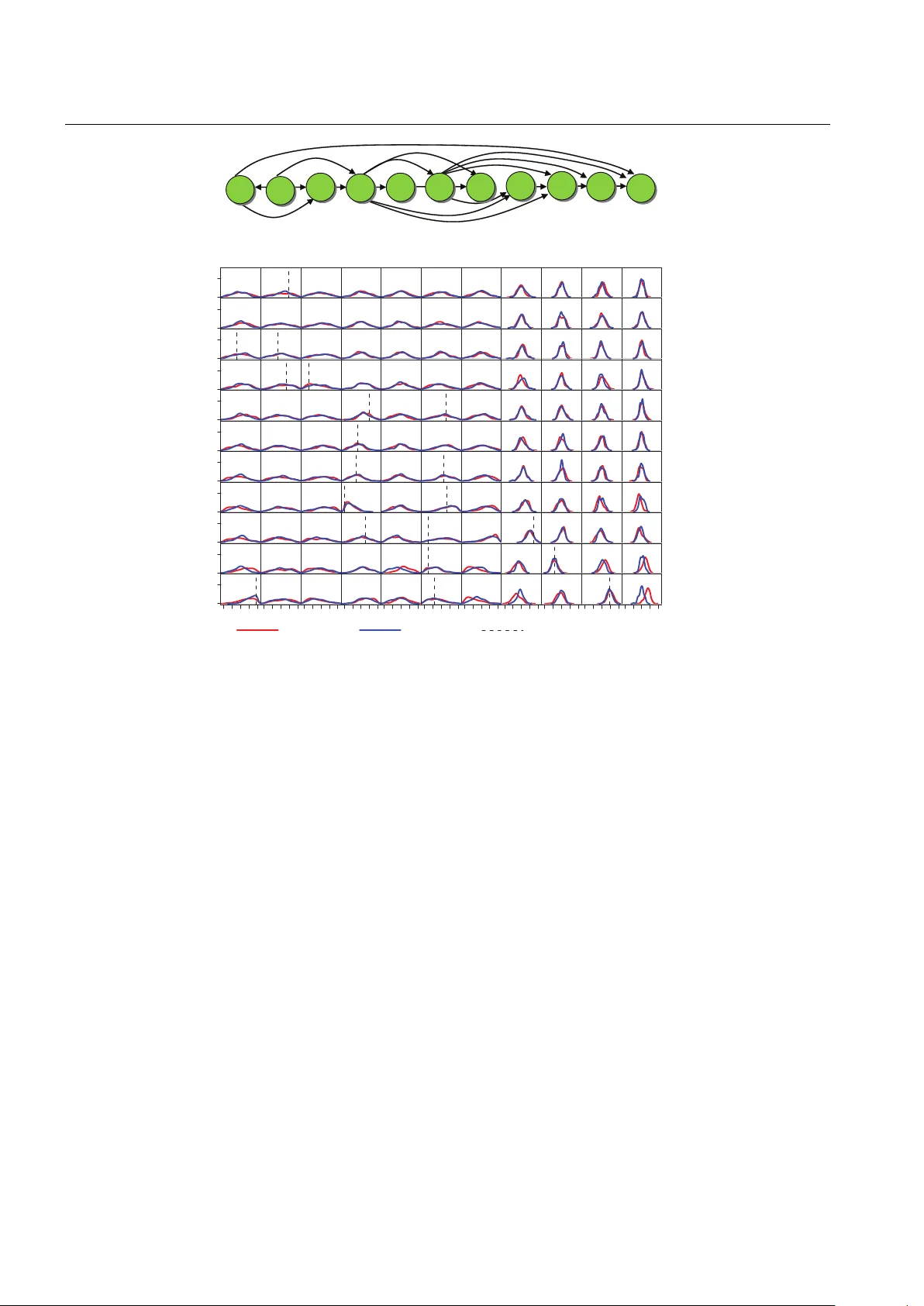
Submitted man uscript Rev erse Engineering Gene Regulatory Net w orks Using Appro ximate Ba y esian Computation Andrea Rau · Florence Jaffr ´ ezic · Jean-Louis F oulley · R. W. Doerge September 7, 2011 Abstract Gene regulatory net wor ks are collections of genes that in teract with one other and with other sub- stances in the cell. By measuring gene expression ov er time using high-throughput tec hnologies, it may be p os- sible to reverse engineer, or infer, the structure of the gene net work in volv ed in a particular cellular pro cess. These gene expression data t ypically ha v e a high dimen- sionalit y and a limited num ber of biological replicates and time p oints. Due to these issues and the complex- it y of biological systems, the problem of reverse engi- neering netw orks from gene expression data demands a sp ecialized suite of statistical to ols and metho dologies. W e prop ose a non-standard adaptation of a simulation- based approach known as Approximate Bay esian Com- puting based on Marko v chain Monte Carlo sampling. This approach is particularly well suited for the in- ference of gene regulatory net works from longitudinal data. The p erformance of this approach is inv estigated via simulations and using longitudinal expression data from a genetic repair system in Escherichia c oli . Keyw ords Appro ximate Ba y esian computation · Gene regulatory netw orks · Longitudinal gene expres- sion · Marko v c hain Monte Carlo A. Rau · R. W. Do erge Department of Statistics, Purdue Univ ersity , W est Lafay ette, IN, USA A.Rau · F. Jaffr´ ezic and J.-L. F oulley INRA, UMR 1313 GABI, Jouy-en-Josas, F rance R. W. Do erge Department of Agronomy , Purdue Univ ersity , W est Lafa yette, IN, USA T el.: +001-765-494-3141 F ax: +001-765-494-0558 E-mail: do erge@stat.purdue.edu 1 Introduction The dev elopment of high-throughput technologies, such as microarrays and next-generation sequencing, has en- abled large-scale studies to simultaneously assa y the expression levels of thousands of genes ov er time. How- ev er, in spite of the abundance of data obtained from these technologies, it can b e very difficult to unrav el the patterns of expression among groups of genes, often re- ferred to as gene regulatory net works (GRN; F riedman, 2004; Wilkinson, 2009). Within GRN, genes in teract with one another indirectly through proteins known as transcription factors (TF), which con trol the transfer of information during transcription by activ ating or re- pressing a ribonucleic acid (RNA) p olymerase, and th us affect the lev el of gene expression (Figure 1). A GRN can thus b e describ ed as the interactions that o ccur (indirectly through messenger RNA and TF) within a collection of interconnected genes. In longitudinal studies of gene expression, the num- b er of samples (i.e., biological replicates or time p oints) collected is typically far outw eighed by the num ber of observ ed genes. Because of the exponentially large n um- b er of p ossible gene-to-gene interactions, reverse engi- neering GRN from longitudinal studies actually ampli- fies the “large p small n ” paradigm. In addition, b ecause gene-to-gene interactions coincide with reactions in the cellular environmen t, the netw ork structure can itself b e v ery complex. F or this reason, standard statistical tec h- niques cannot b e used to infer GRN from gene expres- sion data, and a sp ecialized suite of statistical metho d- ologies hav e b een developed. Among these metho ds, a framework known as Dynamic Ba yesian Netw orks (DBN) has seen wide application in the con text of GRN (Husmeier, 2003; Rangel et al., 2004; Beal et al., 2005; Rau et al., 2010). A DBN uses time-series measure- 2 Andrea Rau et al. DNA Gene 1 Gene 2 Gene 3 Gene 4 TF binding site in promoter region Coding DNA (gene) Transcrip!on factor 1 2 3 4 Fig. 1 A simple gene regulatory netw ork made up of four genes. Each gene is transcrib ed and translated in to a tran- scription factor (TF) protein, which in turn regulates the ex- pression of other genes in the netw ork by binding to their resp ectiv e promoter regions (Sc hlitt and Brazma, 2007). The gene regulatory netw ork ma y be represen ted using the graph in lo w er righ t corner, made up of four nodes (genes) and fiv e edges (in teractions among the genes). Image taken from Rau (2010) men ts on a set of random v ariables to c haracterize their in teractions ov er time. T o av oid an explosion in mo del complexit y , a time-homogeneous Mark ov mo del is typ- ically used (Husmeier et al., 2005). This restriction im- plies that gene-to-gene in teractions are constant across time and that biological samples are taken at equidis- tan t time p oints. Within the framework of DBN, the Bay esian paradigm is particularly well-suited to the inference of GRN for a num b er of reasons. First, the num b er of p ossible net- w ork structures increases exponentially as the n um- b er of genes increases (Husmeier et al., 2005). As a large num b er of netw ork structures may yield similarly high likelihoo ds, attempting to infer a single globally optimal structure may b e meaningless. In such cases, p osterior distributions of gene-to-gene in teractions ma y b etter characterize a GRN. Second, by examining the shap e of the p osterior distributions within p ortions of a GRN, additional information may b e gleaned ab out the structure and inferabilit y of sp ecific gene-to-gene in- teractions, as well as the system as a whole. Finally , a Ba yesian framework allows a priori knowledge to be en- co ded in the prior distribution structure. Prior kno wl- edge may refer to certain features of the top ology of a GRN (e.g., sparsit y in the netw ork structure or the maxim um num ber of regulators p er gene) and to prior biological information ab out well-c haracterized path- w ays from bioinformatics databases. Unless restrictiv e assumptions are made ab out the dynamics of the system (e.g., Gaussian prior distri- butions for gene-to-gene interactions), the likelihoo d function of a GRN may b e in tractable or difficult to calculate. In such cases, sampling-based approximate Ba yesian computation (ABC) metho ds can allow Bay esian inference to b e adopted (Pritchard et al., 1999; Beau- mon t et al., 2002; Marjoram et al., 2003) when simu- lation from the mo del is straightforw ard. The first im- plemen tation of an ABC algorithm was introduced b y Pritc hard et al. (1999). In this approach, using parame- ter v alues simulated from a prior distribution, data are sim ulated and compared to the observed data. When the simulated and observ ed data are sufficiently “close”, as determined by a distance function ρ ( · ) and tolerance  , the parameter v alues are accepted (Beaumont et al., 2002). The algorithm is approximate when  > 0, and its output amoun ts to simulating from the prior when  → ∞ . F or 0 <  < ∞ , the algorithm results in a sample of parameters from an approximate p osterior distribution. Because a naive application of ABC metho ds can b e time-consuming and inefficient, a v ariet y of exten- sions hav e b een prop osed in recent years. F or high- dimensional data, Beaumont et al. (2002) found that using summary statistics to compare simulated and ob- serv ed data, rather than the data p oin ts themselves, en- ables a reduction of the data without negatively impact- ing the approximation. Several adaptations of ABC al- gorithms hav e also b een prop osed based on Mon te Carlo tec hniques. F or instance, Marjoram et al. (2003) ex- tended the ABC algorithm to work within the Marko v c hain Mon te Carlo (MCMC) framework without the use of likelihoo ds. In this approach, which we refer to as ABC-MCMC, parameters are prop osed from a tran- sition distribution (e.g., a random walk) and subse- quen tly used to simulate data. Sisson et al. (2007) used a Sequential Monte Carlo technique (SMC-ABC) to propagate a p opulation of parameters through a se- quence of in termediary distributions to obtain a sample from the approximate p osterior distribution. In related w ork Beaumont et al. (2009) applied an adaptive se- quen tial technique known as Population Mon te Carlo (PMC) to the general ABC algorithm to impro v e its ef- ficiency through iterated imp ortance sampling. F urther recen t implementations of ABC algorithms can also b e found in, e.g., Leuenberger and W egmann (2009) and Dro v andi and P ettitt (2010). In this work, we prop ose an extension of the ABC- MCMC algorithm to enable the inference of GRN from time-course gene expression data. Our approach en- ables Bay esian inference without restrictive assump- tions ab out the distribution of gene-to-gene interac- tions within a netw ork. The resulting approximate pos- terior distributions of interactions within the netw ork ha ve the added adv an tage of providing salient informa- tion ab out the inferability of the biological system as a whole. Although there hav e b een some recen t develop- Reverse Engineering Gene Net works Using ABC 3 men ts in netw ork inference using ABC metho ds, e.g., to compare the evolution of protein-protein interaction net works (Ratmann et al., 2007, 2009) and to conduct mo del selection for systems based on ordinary differ- en tial e quations (T oni et al., 2009; T oni and Stumpf, 2010), to our knowledge this is the first application of ABC metho ds in reverse engineering the unknown structure of a gene regulatory netw ork from gene ex- pression data. 2 Approximate Bay esian Computation for Net w orks Let Y b e a set of observed gene expression data for P genes at T equally-spaced time p oin ts, where y t = ( y 1 t , . . . , y P t ) 0 represen ts the gene expression measure- men ts at time t . In this work, we consider tw o related c haracterizations of a GRN: an adjacency matrix G , and a parameter matrix Θ . F or the former, let G be a P × P matrix suc h that G ij = 1 if gene j regulates gene i , and G ij = 0 otherwise. F or the latter, w e define Θ as the P × P parameter matrix of a GRN, where θ ij represen ts the relationship b et w een gene j at time t − 1 and gene i at time t . F or this matrix, a v alue of θ ij = 0 indicates that gene j do es not regulate gene i ; if θ ij > 0 ( θ ij < 0 resp ectively), gene j activ ates (re- presses) gene i . Note that P ( θ ij = 0 | G ij = 0) = 1, and P ( θ ij = 0 | G ij = 1) = 0. W e will further discuss the si- m ultaneous use of the matrices Θ and G in Section 2.5. Our ob jective in this work is to determine which gene-to-gene in teractions within the GRN may b e in- ferred, based on their appro ximate p osterior distribu- tions. T o accomplish this, we first in tro duce the Bay esian mo del used to mo del the time-course gene expression data Y and corresp onding gene regulatory netw ork Θ . After motiv ating the use of ABC metho ds in this con- text, we then introduce the ABC-MCMC algorithm of Marjoram et al. (2003) in greater detail, and describ e our mo difications for reverse engineering GRN. 2.1 Bay esian Mo del 2.1.1 Likeliho o d sp e cific ation F or a given gene regulatory netw ork Θ , we mo del the time-course gene expression data as a time-homogeneous Mark ov mo del Y ∼ Y t f ( y t ; y t − 1 , Θ ) . (1) with the conv ention that y 0 = 0. Several authors (e.g., Beal et al., 2005; Opgen-Rhein and Strimmer, 2007; Wilkinson, 2009) hav e found that simple, linear mo d- els can in some cases yield go o d appro ximations of the dynamics o ccurring within complicated biological sys- tems. T o this end, one simple y et effective choice for the density f in Equation (1) is a first-order vector au- toregressiv e (V AR(1)) mo del: y t = Θ y t − 1 + e t (2) where e t is an error term satisfying E ( e t ) = 0 , E ( e t e 0 t ) = Σ (a P × P p ositive definite cov ariance matrix), and E ( e t e 0 t 0 ) = 0. In previous w ork (e.g., Beal et al., 2005; Rau et al., 2010), the errors e t ha ve additionally b een assumed to follow a normal distribution, e t ∼ N (0 , Σ ). In this work, we do not imp ose any particular form for the distribution of the errors e t b ey ond the assumptions on the first tw o moments previously men tioned. 2.1.2 Network Prior Distributions T o fully define the Bay esian model used for Y , we m ust also sp ecify the prior distributions for the adjacency matrix G and parameter matrix Θ , π ( G ) and π ( Θ | G ). In a GRN, as the num ber of genes ( P ) in a netw ork in- creases, the num b er of p ossible interactions within the net work quickly increases ( P × P ). As a large num ber of genes may interact simultaneously with one another in very sophisticated regulatory circuits, the netw ork top ology itself may b e quite complicated. Even so, cer- tain prop erties of biological netw orks can b e useful in limiting the supp ort of the prior distribution to realistic net work top ologies. In particular, most genes are reg- ulated just one step a w ay from their regulator (Alon, 2007), and gene netw orks tend to b e sparse, with a lim- ited num b er of regulator genes (Leclerc, 2008). In keeping with these biological h ypotheses, w e elect to use uninformative prior distributions with some re- strictions for b oth π ( G ) and π ( Θ | G ). W e restrict the n umber of regulators for each gene (referred to as the fan-in for each gene in the netw ork). Because GRN are kno wn to b e sparse, w e choose the prior on the ad- jacency matrix, π ( G ), to be uniform ov er all p ossible structures, sub ject to a constraint on the maxim um fan-in for each gene in the netw ork, as has b een sug- gested (F riedman, 2000; Husmeier, 2003; W erhli and Husmeier, 2007). This restriction is supp orted by the biological literature, as genes do not tend to b e syn- c hronously regulated by a large num b er of genes (Leclerc, 2008). F or the parameter prior π ( θ ij | G ij = 1), we use a uniform distribution, where the b ounds are chosen to represen t a realistic range of interaction magnitudes in GRN. In this w ork, w e use b ounds of -2 and 2 for all θ ij , as these corresp ond to strong repression and activ ation effects, resp ectiv ely . 4 Andrea Rau et al. 2.2 ABC Motiv ation Giv en the likelihoo d and prior distributions defined in the previous section, our goal is to reverse engineer a GRN from observ ed expression data Y via the p osterior distribution π ( Θ , G | Y ) ∝ f ( Y | Θ ) π ( Θ | G ) π ( G ) . In some cases, the error term e t included in the like- liho od in Equation (2) is assumed to follow a well- kno wn distribution (e.g., a Normal distribution). This h yp othesis would enable straightforw ard calculation of the likelihoo d, and in turn, the p osterior distribution π ( Θ | Y ), whether through explicit calculation or a stan- dard MCMC sampler. How ev er, in this work we do not imp ose a specific distributional form for e t , and as suc h, the lik elihoo d f ( Y | Θ ) cannot be ev aluated. It is exactly in situations such as this that ABC metho ds hav e b een successfully developed and applied in recent y ears. Simple ABC rejection metho ds (e.g., Pritchard et al. (1999)) hav e the adv an tage of b eing easy to co de and generating indep enden t observ ations, but can b e ex- tremely time consuming and inefficient, particularly in the case of GRN. T o illustrate, we applied the follow- ing simple ABC rejection metho d to sample from the appro ximate p osterior distribution π ( Θ , G | Y ): 1. Generate G and Θ from π ( G ) and π ( Θ | G ), resp ec- tiv ely . 2. Generate one-step-ahead predictors y ? t from mo del 2, giv en y t − 1 and Θ ? (see Section 2.4 for a discussion of this simulation strategy). 3. Calculate the distance ρ ( Y , Y ? ) b etw een Y and Y ? . 4. Accept ( Θ ? , G ? ) if ρ ≤  , where  is chosen as de- scrib ed in Section 2.6. Using this algorithm, only 5 prop osed netw orks ( Θ ? , G ? ) are accepted out of a total of 1 × 10 7 prop osals (data not sho wn). Because suc h an approach is b oth inefficient and unpractical, w e fo cus instead on the ABC-MCMC approac h of Marjoram et al. (2003). 2.3 ABC Marko v Chain Monte Carlo for Netw orks The ABC-MCMC algorithm (Marjoram et al., 2003) mak es use of the standard Metrop olis-Hastings scheme (Hastings, 1970) to obtain samples from the approx- imate p osterior distribution π ( Θ , G | ρ ( Y ? , Y ) <  ). T o accomplish this, matrices Θ ? and G ? are prop osed based on a prop osal distribution q ( ·|· ) and subsequently used to simulate data Y ? based on a given mo del f ( ·| Θ ? ). Sim ulated and observed data are compared using a dis- tance function ρ ( · ) and tolerance  , and prop osed pa- rameters are accepted with probability α = min  1 , π ( Θ ? , G ? ) q ( Θ i , G i | Θ ? , G ? ) π ( Θ i , G i ) q ( Θ ? , G ? | Θ i , G i ) 1 ( ρ ( Y ? , Y ) <  )  where 1 ( · ) is an indicator function that replaces the lik eliho od, and π ( · ) represents the prior distributions of ( Θ , G ). Under suitable regularit y conditions (Marjoram et al., 2003), it is straightforw ard to show that the sta- tionary distribution of the chain is indeed the approx- imate p osterior distribution. If  is sufficien tly small, then this distribution will b e a go o d approximation to the true p osterior distribution π ( Θ , G | Y ). Ho w ever, a balance must b e achiev ed b etw een a small enough tol- erance to obtain a goo d approximation to the p oste- rior and a large enough tolerance to allow for feasible computation time. Bortot et al. (2007) prop osed a fur- ther adaptation of ABC-MCMC for the purp ose of im- pro ving its mixing prop erties using data augmentation tec hniques, kno wn as the ABC-MCMC augmen ted al- gorithm. Sp ecifically , the parameter space is augmented with the tolerance  , which is treated as a mo del param- eter with its own pseudo-prior distribution. Although this algorithm alleviates the problem of insufficien t mix- ing, since larger v alues of  may b e accepted, it typi- cally requires a muc h larger num b er of iterations than the original ABC-MCMC algorithm. Adapting the ABC-MCMC algorithm of Marjoram et al. (2003) to the con text of GRN requires t wo impor- tan t considerations to b e taken into account: 1) com- putationally efficient metho ds for simulating data Y ? from a known GRN (defined by its parameter matrix Θ ? ), and 2) an appropriate prop osal distribution q ( ·|· ) for b oth the netw ork structure and parameters. W e re- fer to the algorithm incorp orating these adaptations as the ABC for Net works (ABC-Net) metho d. F or clarity , although we limit this discussion to data with a single biological replicate, the extension to multiple replicates is straightforw ard. 2.4 Simulating Data for Gene Netw orks within ABC One of the most imp ortant considerations in adapting the ABC-MCMC algorithm to the inference of GRN is identifying an efficient sim ulator for prop osed net- w ork parameter matrix Θ ? . Broadly , we simulate gene expression at time t as a function of gene expression at the previous time p oint and the proposed parame- ter matrix Θ ? using a V AR(1) mo del as in Equation 2. Sp ecifically , after setting y ? 1 = y 1 , we exploit the Reverse Engineering Gene Netw orks Using ABC 5 Mark ov prop ert y of the V AR(1) mo del to obtain one- step-ahead predictions (i.e., fitted v alues) of gene ex- pression at time p oints t = 2 , . . . , T : y ? t = Θ ? y t − 1 . (3) Note that the one-step-ahead predictions for y t are made using the observed data y t − 1 , and not the sim ulated data y ? t − 1 . That is, we simulate data deterministically b y calculating the exp ected v alue of gene expression at eac h time p oin t given the netw ork structure and ob- serv ed expression v alues at the previous time p oint, rather than incorp orating an estimate of noise in the sim ulated data. W e are aw are that the deterministic simulation pro- cedure discussed ab o v e is somewhat unconv en tional in the ABC literature, primarily since it do es not incor- p orate an estimate of noise in the simulated data Y ? . More classically , rep eated sampling is used to control the v ariability of the data by simulating several noisy datasets { Y ? 1 , . . . , Y ? M } for a given net work Θ ? , with M > 1. Keeping this in mind, adding no noise can b e seen as the limiting case of M > 1 replications of the dataset generated from the same Θ , as advocated in some ABC pro cedures (Del Moral et al., 2009). In our case, the choice to use the one-step-ahead predictors as in Equation (3) is a practical one. More sp ecifically , b e- cause the time-series expression data are mo deled as a V AR(1) pro cess, we found that adding noise at early time p oin ts simply had the effect of inducing wide dis- crepancies at later time p oints, as incorrect error terms comp ounded throughout the simulated time series. This had the effect of creating large distances ρ ( Y , Y ? ), even when the true netw ork Θ w as used to generate Y ? . Finally , the appropriateness of using a V AR(1) sim- ulator, Equation (3), is largely dep endent on the noise presen t in observed data, as w ell as the adequacy of the assumption of time-inv arian t, first-order autoregres- siv e dynamics for complicated GRN. In the absence of more detailed information ab out the underlying net- w ork, it ma y b e reasonable to use a s imple mo del such as the V AR(1) to generate simulated data. W e note that the ABC-Net algorithm has the flexibilit y to in- corp orate arbitrary models as data simulators, provided they are computationally efficien t. F or instance, in some cases second-order models, nonlinear models, linear dif- feren tial equations, draws from a Dirichlet pro cess, or Mic haelis-Menten kinetics ma y more aptly describ e the dynamics of a particular GRN; in these cases, the ap- propriate sim ulator model would b e used in place of Equation (3). 2.5 Two-Step Netw ork Prop osal Distributions Another imp ortant consideration is the prop osal distri- bution q ( ·|· ) that defines the transition from the current prop osal for a GRN to an up dated prop osal. Based on the current v alues of G and Θ , a tw o-step prop osal dis- tribution is used to pro duce new samples G ? and Θ ? for the adjacency and parameter matrices, resp ectively . In this context, the adjacency matrix G ma y b e viewed as an auxiliary v ariable (Damien et al., 1999), which is in tro duced to simplify the Marko v chain Mon te Carlo algorithm. As such, the joint distribution of G and Θ ma y b e seen as a completion of the marginal density of Θ (Rob ert and Casella, 2004) which facilitates simula- tion within the MCMC algorithm. In the first step, one of three basic mov es (Husmeier et al., 2005) is applied to the current adjacency matrix G i : adding an interaction (i.e., changing a 0 to a 1), deleting an interaction (i.e., changing a 1 to a 0), or rev ersing the direction of an interaction (i.e., if G ij = 1 and G j i = 0, exchanging these tw o v alues). If N ( G ) rep- resen ts the neighborho o d size of a particular adjacency matrix G , (i.e., the num b er of other netw ork structures that can b e obtained by applying one of these three ba- sic mov es), the transition probability of the first step is giv en by q ( G ? | G i ) = 1 / N ( G i ). In the second step, the prop osal distribution of Θ , giv en the current v alue Θ i and the up dated adjacency matrix G ? , is defined to b e q ( θ ij | θ i ij , G ? ij ) ∼  0 if G ? ij = 0 N ( θ i ij , σ 2 Θ ) if G ? ij 6 = 0 (4) where σ 2 Θ is the v ariance of the proposal distribution, and σ Θ ma y b e tuned to obtain an empirical acceptance rate b et w een 15% and 50%, as recommended in Gilks et al. (1996). A simple example of the tw o-step prop osal distribution for GRN is shown in Figure 2. It is worth noting that the introduction of the ad- jacency matrix G is not strictly necessary to accom- plish the tw o-step prop osal describ ed ab ov e. F or in- stance, it would b e straightforw ard to define the tar- get with resp ect to a mixture of singular measures, e.g., a dirac mass and a Gaussian density (see Gottardo and Raftery, 2004, for more details). F urthermore, the three prop osal mov es (add, delete, and reverse a net- w ork edge) could b e defined using a mixture of ker- nels that include selection probabilities dep ending on the curren t state. Our primary motiv ation for includ- ing G is based on the approach for learning Bay esian net works in Chapter 2 of Husmeier et al. (2005), whic h clearly distinguishes the netw ork structure (i.e., the set of edges and nodes represen ted b y the adjacency matrix G ) from the netw ork parameters (the matrix Θ ). The 6 Andrea Rau et al. A B C 0 0 0 0 0 2 3 0 0     −       C Θ i = A A B B C Parameter matrix A B C Θ * = A A B B C 0 0 0 0.4 0 0.3 2.7 0 0     −       C Add, delete, reverse edge (Husmeier, 2003) A B C 0 0 0 0 0 1 1 0 0           A A B B C C G i = A B C Adjacency matrix A B C A A B B C G * = A B C 0 0 0 1 0 1 1 0 0           C Gaussian proposal Fig. 2 Example of tw o-step prop osal distribution for GRN. T op row: A netw ork in iteration i of the ABC-Net algorithm ma y b e characterized b oth by its adjacency matrix G i (left) and its parameter matrix Θ i (righ t). The former encodes only the presence (1) or absence (0) of an interaction. The latter enco des additional information ab out the magnitude of a par- ticular interaction, where zeros indicate that an interaction is not present, p ositiv e v alues indicate an activ ation, and nega- tive v alues indicate a repression (interactions with v alues fur- ther aw a y from zero corresp ond to stronger effects). Bottom ro w: An up dated netw ork is prop osed by adding, deleting, or reversing an in teraction in G i to pro duce G ? (left). The parameter matrix Θ i is up dated using a Gaussian prop osal distribution for the nonzero in teractions of G ? to produce Θ ? (righ t). Image taken from Rau (2010) three-mo ve prop osal strategy we apply for the structure of the netw ork is based on this intuitiv e representation, and is rather p opular in Bioinformatics (see e.g., Hus- meier et al., 2005). 2.6 ABC-Net Implementation The output from the ABC-Net algorithm consists of dep enden t samples from the stationary distribution of the chain, f ( Θ , G | ρ ( Y ? , Y ) ≤  ). In practice, because sa ving all iterations from the MCMC run can tak e up a large amount of storage (particularly as the size of the net w ork increases) and consecutive draws tend to b e highly correlated, we thin the chain at every 50 th iteration. Additionally , as with many MCMC metho ds, a burn-in perio d is implemen ted to reduce the impact of initial v alues and to improv e mixing for the c hain. The length b of the burn-in dep ends on the starting v alues of the chain, Θ 0 and G 0 , the rate of conv ergence of the c hain, and the similarity of the transition mechanism of the c hain to the approximate p osterior distribution. W e follow the suggestion of Gey er (1992), setting b to b et w een 1% and 2% of the run length n . W e also implement a “co oling” pro cedure during the burn-in p eriod similar to that used in Ratmann et al. (2007), where acceptance of ( G ? , Θ ? ) is controlled by a decreasing sequence of thresholds, until the minimum pre-set v alue  is reached. Note that temp ering the ac- ceptance threshold  in this w ay reduces the num b er of accepted parameters as the num ber of iterations in- creases. This co oling scheme also addresses the p o or mixing often observed in the ABC-MCMC algorithm, as larger tolerances in the early iterations of the burn-in are asso ciated with higher acceptance rates. A total of 200 iterations are run for each of ten co oled threshold v alues, and the burn-in p erio d is rep eated if the em- pirical acceptance rate is less than 1%. This ensures a minim um burn-in p erio d of 2000 iterations, with ad- ditional iterations included for chains affected by po or mixing. Because the ABC-Net algorithm relies on a com- parison b etw een simulated and observed data to av oid a likelihoo d calculation, long chains are required to en- sure the adequacy of the approximation. Although a single long chain could b e run, it is also p ossible to run multiple ov erdisp ersed chains. In practice, we run 10 indep enden t chains of length 1 × 10 6 sim ultaneously (rather than a single chain of length 1 × 10 7 ). This ap- proac h con tributes a t wo-fold b enefit, as calculations can b e p erformed in parallel to impro v e computational sp eed and a conv ergence assessment can b e conducted using the Gelman-Rubin statistic R (Gelman and Ru- bin, 1992). F ollo wing the recommendation in Gilks et al. (1996) we declare chain con v ergence if ˆ R < 1 . 2 for all parameters in Θ . After the chains ha v e conv erged, dra ws corresp onding to the smallest 1% of the distance criterion are retained for inference. 3 Simulation Study Based on the Raf Path wa y In this simulation study , w e focus on four sp ecific as- p ects related to the p erformance of the ABC-Net: the distance function ρ and tolerance  , the sensitivity to prior distribution b ounds, the suitability of the mo del used to generate simulated data when more c omplicated dynamics are at pla y , and the effect of increasing the amoun t of noise presen t in the observed data. T o do so, we fo cus on the Area Under the Curve (A UC) of the Receiver Op erating Characteristic (R OC) curve as an indicator of p erformance, as well as qualitative ex- aminations of the approximate p osterior distributions of in teractions in the net work. T o calculate the AUC , w e retain only the samples corresp onding to the small- est 1% of distances ρ ( Y ? , Y ) for inference. Based on these samples, we calculate the b ounds of the α % cred- ible interv als for each gene-to-gene interaction, where α = { 1 , . . . , 100 } . If the α % credible interv al for a par- ticular interaction do es not contain 0, the gene-to-gene in teraction is declared to be present; otherwise, the in- teraction is declared to b e absen t. In this wa y , b ecause the simulation setting determines which in teractions are truly present and absent, true p ositiv es, false p ositiv es, Reverse Engineering Gene Netw orks Using ABC 7 Fig. 3 The currently accepted gold-standard Raf signalling path wa y (W erhli and Husmeier, 2007), which describes the intera ctions of eleven phosphorylated proteins in primary hu- man immune system cells (Sac hs et al., 2005). Nodes rep- resent the proxy genes of each of the eleven proteins (i.e., the genes that are transcrib ed and translated in to the corre- sp onding proteins), and arrows indicate the direction of signal transduction. Image taken from Rau (2010) true negatives, and false negatives may b e calculated for eac h α , and the AUC may subsequently b e calculated. The v alues of α may b e adjusted for multiple testing, if necessary . 3.1 Simulation Design Rather than defining an arbitrary netw ork Θ , we in- stead mak e use the structure of a well-c haracterized path wa y in human immune system cells in volving the Raf signalling protein (Sachs et al., 2005). W e generate data based on 11 genes, where the adjacency matrix G Raf is defined using the structure of the currently ac- cepted Raf signalling netw ork (Figure 3). If an interac- tion is present from gene j to gene i , we sample θ Raf ij uniformly from the interv al ( − 2 , − 0 . 25) ∪ (0 . 25 , 2), and otherwise θ Raf ij = 0. The b ounds for non-zero gene-to- gene interactions were c hosen to represent a range of mo derate to strong interactions among genes. W e gen- erate one replicate of expression data for each of the 11 genes ov er 20 time p oin ts, using the V AR(1) mo del y t = Θ Raf y t − 1 + z t (5) for t = 1 , ..., T , w here y 1 ∼ N (0 , I ), and z t ∼ N (0 , σ 2 ). F or each simulation, unless otherwise noted, the noise standard deviation is set to σ = 1, the Gaussian pro- p osal standard deviation in Equation (4) is set to σ Θ = 0 . 5, and the maxim um fan-in is constrained to 5 or less. 3.2 Choice of ρ and  The distance function ρ and threshold  are essential comp onen ts to the ABC-Net metho d, as they directly affect the probabilit y that sim ulated data Y ? generated 0.50 0.55 0.60 0.65 0.70 0.75 0.80 AUC 1% 5% 10% 1% 5% 10% 1% 5% 10% 1% 5% 10% Canberra Euclidean Manhattan MVT Distance Function and Threshold Area Under the Curve (By Distance Function and Threshold) Fig. 4 Area Under the Curve (AUC) of the Receiver Op er- ating Characteristic (ROC) curve for four choices of distance functions in the ABC-Net algorithm: Canberra, Euclidean, Manhattan, and MVT distances. Black dots represent the v alue of the AUC for each of five indep endent datasets p er threshold and distance function (with the exception of the MVT distance, which was limited to tw o datasets due to its computational burden). The threshold  was set at the 1%, 5%, and 10% quantiles from 5000 randomly generated net- w orks. Blue lines represent lo ess curves (Cleveland, 1979). Image taken from Rau (2010) b y a netw ork Θ ? are accepted as b eing “close enough” to the observed data. Although there are many po- ten tial options for this distance function, we fo cus on a comparison among the Manhattan, Euclidean, Can- b erra, and Multiv ariate Time-Series (MVT; Lund and Li, 2009) distances (see App endix). F or each choice of ρ , we prop ose a heuristic metho d where 5000 ran- domly generated netw orks are used to simulate data, and the corresp onding distances ρ ( Y ? , Y ) are calcu- lated for eac h. Subsequently ,  is set to b e either the 1%, 5%, or 10% quantile of these distances asso ciated with 5000 randomly generated netw orks. The n um b er of randomly generated netw orks was chosen based on a set of preliminary sim ulations that indicated that the quantiles for the corresp onding distances ρ ( Y ? , Y ) seemed to stabilize for 5000 or more net w orks (data not sho wn). F or larger netw orks, further exploratory simu- lations ma y need to b e p erformed to ensure that this n umber is not to o small. Each combination of ρ and  was rep eated ov er five indep enden t datasets in order to include an assessment of their v ariability (only tw o datasets were sim ulated for the MVT distance due to its computational burden). Eac h distance function under consideration calcu- lates and p enalizes differences b et w een simulated and observ ed data in a different w ay . In particular, the b e- ha vior of the MVT function app ears to differ from that 8 Andrea Rau et al. 1 2 3 4 5 1 2 3 4 5 Gelman−Rubin Statistic 1 2 3 4 5 1 2 3 4 5 1 2 3 4 5 Convergence Assessment by Prior Bounds (−2,2) (−3,3) (−5,5) (−10,10) Prior Bounds and Replicate Number Convergence cutoff (= 1.2) Fig. 5 Gelman-Rubin statistics ( ˆ R ) for eac h replicate of four cho ices of b ounds on the prior distribution π ( Θ | G ). The black dotted line indicates a v alue of ˆ R = 1 . 2, the cutoff at which con vergence is declared among ten indep endent chains in the ABC-Net algorithm. Image taken from Rau (2010) of the other distance functions, with muc h low er A UC v alues for each com bination of ρ and  (Figure 4). The Can b erra, Euclidean, and Manhattan distances all ap- p ear to b e on par with one another, particularly when  is set at the 1% quantile of distances. How ev er, based on the criterion of AUC alone, there do es not seem to b e strong evidence that fav ors one choice among the Can b erra, Euclidean, and Manhattan distances, partic- ularly for a cutoff of  = 1%. That is, although the MVT distance is a p o or c hoice of distance function within the ABC-Net algorithm, the remaining distances yield simi- lar results. Because it enjo ys a slight adv an tage ov er the Manhattan and Canberra distances in terms of compu- tation time, we use the Euclidean distance with  set to the 1% threshold for the remainder of the simulations. 3.3 Sensitivity to prior distribution b ounds Although the prior b ounds (-2 and 2) for π ( Θ | G ) are reasonable for the context of GRN, we also consider the following bounds: (-3,3), (-5,5), and (-10,10). These in terv als include somewhat “unrealistic” v alues for Θ , but are more diffuse (and hence less informative). The greatest effect of using less informative prior distribu- tions is in terms of the conv ergence of the ten indep en- den t c hains, as assessed by the Gelman-Rubin statistic (Figure 3.2). This is most evident for prior b ounds of (-10,10), where a large num b er of interactions exceed the conv ergence c utoff of 1.2 by a large amoun t. It is p erhaps unsurprising that wider prior b ounds lead to problems in chain mixing and conv ergence, and thus highligh ts the need for w ell-chosen prior b ounds for the inference of GRN. W e also consider the effect of the c hoice of prior b ounds on the shap e of the appro ximate p osterior dis- tributions in the netw ork. In Figure 6, a graphical ma- trix of the marginal approximate p osterior distribu- tions of each interaction in the netw ork is giv en for prior b ounds (-2,2). As may b e exp ected, the approxi- mate p osteriors are generally more diffuse when wider prior b ounds are used. Ho w ev er, regardless of the c hoice of prior b ound, some gene-to-gene in teractions consis- ten tly hav e very flat (diffuse) approximate posterior d is- tributions (e.g., those in the Pip3 column), while oth- ers tend to b e consisten tly p eak ed (e.g., those in the Erk column). W e refer to gene-to-gene in teractions with these t w o c haracteristics as “flexible” and “rigid”, re- sp ectiv ely . Interestingly , in this sim ulation, the most rigid interactions app ear to corresp ond to regulators that are furthest downstream in the sim ulated pathw a y (Mek, Erk, and Akt), while those furthest upstream ap- p ear to be the most flexible. In the con text of the ABC- Net metho d, this suggests that rigid interactions (e.g., Mek → Erk) in Θ ? m ust take on v alues within a tigh t in terv al in order to generate sim ulated data Y ? that are close (in terms of ρ and  ) to the observed data Y . Con versely , flexible in teractions (e.g., Pip3 → Pip3) can tak e on v alues within a muc h wider interv al without negativ ely affecting the pro ximity of simulated and ob- serv ed data. Thus, it is lik ely that the mo del is most sensitiv e to parameters with narrow credible in terv als (rigid interactions) and least sensitive to those that can- not accurately b e localized (flexible interactions) by the appro ximate p osterior distribution (T oni et al., 2009). That is, it app ears that some interactions may intrin- sically b e easy to infer even with relatively wide prior b ounds, while others cannot b e accurately determined ev en with reasonable prior distribution b ounds. 3.4 Suitability of V AR(1) Simulator The applicability of the ABC-Net metho d to real GRN relies heavily on its ability to accurately simulate data for a given net work structure. It is feasible that real biological systems do not follow a V AR(1) mo del, and in fact, that they arise from very complicated, nonlin- ear relationships. T o assess how the ABC-Net metho d p erforms when observed data Y are actually gener- ated from more complicated mo dels, we fo cus on four mo dels (T able 1): a first-order nonlinear V AR mo del (V AR-NL(1)), a second-order V AR mo del (V AR(2)), a second-order nonlinear V AR mo del (V AR-NL(2)), and an ordinary differential equation (ODE). F or the V AR mo dels, Θ Raf 1 and Θ Raf 2 w ere each defined using the Reverse Engineering Gene Netw orks Using ABC 9 −2 0 2 Pkc −2 0 2 Raf −2 0 2 Mek −2 0 2 Erk −2 0 2 Pka Pkc Raf Mek Erk Pka −2 0 2 Akt P38 Jnk Plc γ Akt Pip3 Pip2 −2 0 2 P38 −2 0 2 Jnk −2 0 2 Plc γ 0 1 0 1 0 1 0 1 0 1 0 1 −2 0 2 0 1 0 1 0 1 0 1 Pip3 0 1 −2 0 2 Pip2 Parameter value Density Approximate Posterior Distributions Pip3 Plcγ Pip2 Pkc P38 Pka Jnk Raf Mek Erk Akt Fig. 6 The structure of the true Raf signalling pathw ay , Θ Raf , and a graphical matrix of the marginal approximate p osterior distributions for every interaction in the netw ork, with prior b ounds (-2,2). Each element of the graphical matrix corresponds to the same element of Θ Raf , i.e., the density in the second row and first column corresp onds to θ Raf 21 (Pip3 → Plc γ ). The x-axis of eac h plot represents the v alues of each parameter θ Raf ij , and the y-axis represents the corresponding density . Black dotted lines are included on plots where θ Raf ij 6 = 0 at the true v alue. Image taken from Rau (2010) structure of the Raf signalling netw ork, where exist- ing interactions were sampled uniformly from the in- terv al ( − 2 , − 0 . 25) ∪ (0 . 25 , 2) and otherwise set to 0. F or the ODE m odel, co efficien ts were randomly dra wn from a U ( − 1 , 1) distribution and initial v alues for all genes w ere set to 1. After solving the ordinary differ- en tial equations for time p oints t = 1 , . . . , 20, random noise sampled from N (0 , 1) w as added to eac h measure- men t at each time p oint. It is not surprising that the ABC-Net has the b est p erformance in terms of A UC for the V AR(1) mo del, as the data Y are generated with the same mo del that is used to simulate Y ? (Figure 7). F or the other simu- lator mo dels, the p erformance of the algorithm notice- ably declines, with the low est AUC v alues observed for the tw o second-order mo dels, V AR(2) and V AR-NL(2). The nonlinear first-order V AR mo del shows wide v ari- abilit y in its results, ranging from an AUC of just ov er 0.40 to ov er 0.70. Of the alternativ e mo dels, the ordi- nary differential equation app ears to hav e the highest p erformance in terms of A UC. As a final note concern- ing the p erformance of the ABC-Net algorithm when alternativ e mo dels are used to generate Y , recall that the simulator describ ed in Section 2.4 has the flexibil- it y to incorporate alternativ e models, pro vided they are computationally efficien t. In this resp ect, the V AR(1) mo del may b e viewed as a kind of robust null mo del to apply when nothing is precisely known ab out the dy- namics of a particular system. Ho wev er, in cases where other mo dels are known to b etter fit a given set of data (e.g., a second order or non-linear model), the ABC-Net metho d can b e adapted accordingly . 3.5 Effect of Noise in Observed Data W e exp ect that increasing amounts of noise in the ob- serv ed data (i.e., σ in Equation 5) lead to reduced p er- formance for the ABC-Net algorithm, particularly since the V AR(1) simulator uses one-step ahead predictors to 10 Andrea Rau et al. T able 1 Alternative mo dels used to generate observed data Y : an ordinary differential equation (ODE), a second-order V AR model (V AR(2)), a first-order nonlinear V AR mo del (V AR-NL(1)), and a second-order nonlinear V AR mo del (V AR-NL(2)) Mode l Netw ork Equations to Generate Y V AR-NL(1) y 1 = z 1 y t = Θ Raf 1 y − 1 t − 1 + z t , for t = 2 , . . . , T z t ∼ N (0 , 1) for t = 1 , . . . , T V AR(2) y 1 = z 1 y 2 = Θ Raf 1 y 1 + z 2 y t = Θ Raf 1 y t − 1 + Θ Raf 2 y t − 2 + z t , for t = 3 , . . . , T z t ∼ N (0 , 1) for t = 1 , . . . , T V AR-NL(2) y 1 = z 1 y 2 = Θ Raf 1 y − 1 t − 1 + z 2 y t = Θ Raf 1 y − 1 t − 1 + Θ Raf 2 y t − 2 + z t , for t = 3 , . . . , T z t ∼ N (0 , 1) for t = 1 , . . . , T ODE y 0 Pkc = 0 . 18 y Plc γ − 0 . 75 y Pip2 y 0 Raf = − 0 . 28 y Pkc + 0 . 62 y Pk a y 0 Mek = 0 . 63 y Pkc − 0 . 97 y Raf − 0 . 52 y Pk a y 0 Erk = 0 . 70 y Mek − 0 . 94 y Pk a y 0 Pk a = 0 . 31 y Pkc y 0 Akt = 0 . 28 y Erk + 0 . 60 y Pk a + 0 . 92 y Pip3 y 0 P38 = − 0 . 19 y Pkc − 0 . 32 y Pk a y 0 Jnk = 0 . 24 y Pkc + 0 . 98 y Pk a y 0 Plc γ = 0 y 0 Pip3 = − 0 . 28 y Plc γ y 0 Pip2 = 0 . 83 y Plc γ − 0 . 98 y Pip3 0.40 0.45 0.50 0.55 0.60 0.65 0.70 0.75 AUC VAR(1) VAR−NL(1) VAR(2) VAR−NL(2) ODE Model Type Area Under the Curve (By Model) Fig. 7 Area Under the Curve (AUC) of the Receiver Op- erating Characteristic (ROC) curve for five different mo del cho ices to generate Y : V AR(1), V AR-NL(1), V AR(2), V AR- NL(2), and ODE. Black dots represent the v alue of the AUC for each of five independent datasets p er b ound. Image taken from Rau (2010) sim ulate data based on a giv en netw ork Θ ? . T o ev aluate this, we consider σ = { 0 , 0 . 1 , 0 . 25 , 0 . 5 , 0 . 75 , 1 , 1 . 5 , 2 , 3 , 5 } , 0.60 0.65 0.70 0.75 0.80 0.85 0.90 Observed Noise Standard Deviation AUC 0.00 0.50 1.00 1.50 2.00 3.00 5.00 Area Under the Curve (By Observed Noise) Fig. 8 Scatterplots of the Area Under the Curve (AUC) of the Receiv er Op erating Characteristic (ROC) curve for the ABC-Net algorithm, with differing v alues of noise standard deviation σ (0, 0.1, 0.25, 0.5, 0.75, 1, 1.5, 2, 3, 5). Five datasets w ere generated for each v alue of noise standard deviation. The blue line represents a loess curve (Cleveland, 1979). Image tak en from Rau (2010) where z t ∼ N (0 , σ ). The AUC results (Figure 8) in- dicate that the presence of increasing noise o ver the in vestigated range do es seem to nega tiv ely affect the p erformance of the ABC-Net algorithm, although only for relativ ely large v alues of σ (e.g., σ = 5). As the noise standard deviation increases, it is not surprising that the performance of the algorithm deteriorates, since the one-step-ahead predictors fall increasingly further from the observed data (even when the true net w ork is used). W e also examine the approximate p osterior distri- butions of the netw ork for tw o different v alues of noise standard deviation, σ = 0 . 5 and σ = 5 (Figure 9). F or the most part, p osterior distributions for b oth σ = 0 . 5 and σ = 5 seem to hav e the same general shap e, with some o ccasional discrepancies (e.g., Akt → Akt and Akt → Erk). In addition, as in previous simulations, we note once again the marked difference in p osterior dis- tributions b etw een rigid interactions (p eak ed distribu- tions) and flexible interactions (diffuse distributions). Regardless of the amoun t of noise incorporated into the sim ulated data for the Raf signalling pathw a y , the ap- pro ximate p osterior distributions for the upstream and do wnstream p ortions of the net w ork are consistently flexible and rigid, resp ectiv ely . This seems to indicate that some interactions are intrinsically easier to infer (ev en in the presence of increased noise), while oth- ers cannot b e accurately determined regardless of the amoun t of noise in the data. As suc h, the flexibility and rigidit y of interactions in a given system likely plays an Reverse Engineering Gene Netw orks Using ABC 11 Pip3 Plcγ Pip2 Pkc P38 Pka Jnk Raf Mek Erk Akt −2 0 2 Pkc −2 0 2 Raf −2 0 2 Mek −2 0 2 Erk −2 0 2 Pka Pkc Raf Mek Erk Pka −2 0 2 Akt P38 Jnk Plc γ Akt Pip3 Pip2 −2 0 2 P38 −2 0 2 Jnk −2 0 2 Plc γ 0 1.5 0 1.5 0 1.5 0 1.5 0 1.5 −2 0 2 0 1.5 0 1.5 0 1.5 0 1.5 0 1.5 Pip3 0 1.5 −2 0 2 Pip2 SD = 5 SD = 0.5 True Parameter value Density Approximate Posterior Distributions Fig. 9 The structure of the true Raf signalling pathw ay , Θ Raf , and a graphical matrix of the marginal approximate p osterior distributions for every interaction in the netw ork, for σ = 0 . 5 and 5. Each element of the graphical matrix corresp onds to the same element of Θ Raf , i.e., the density in the second row and first column corresp onds to θ Raf 21 (Pip3 → Plc γ ). The x-axis of each plot represen ts the v alues of each parameter θ Raf ij , and the y-axis represents the corresp onding density . Red and blue lines correspond to results obtained with σ = 5 and σ = 0 . 5, resp ectiv ely . Black dotted lines are included on plots where θ Raf ij 6 = 0 at the true v alue. Image taken from Rau (2010) imp ortan t role in the global inferabilit y of the netw ork structure. 4 Application to S.O.S. DNA Repair System in Escherichia c oli The S.O.S. DNA repair system in the Escherichia c oli bacterium is a well-kno wn gene netw ork that is resp on- sible for repairing DNA after damage. The full netw ork is made up of ab out thirty genes working at the tran- scriptional level. The b ehavior of these genes in the presence of DNA damage has b een w ell characterized (Ronen et al., 2002). Sp ecifically , under normal condi- tions a master repressor called lexA represses the ex- pression of the genes resp onsible for DNA repair. How- ev er, when one of the S.O.S proteins (recA) senses DNA damage b y binding to single-stranded DNA, it becomes activ ated and pro v okes the auto cleav age of lexA. The subsequen t drop in the levels of lexA susp ends the re- pression of the S.O.S. genes, and these genes b ecome activ ated. Once DNA damage has b een repaired, the lev el of recA drops, whic h allows lexA to reaccum ulate in the cell and subsequently repress the S.O.S. genes. A t this p oint, the cells return to their original state. Although the netw ork itself is quite small, its simple structure allows the cell to react in v ery sophisticated w ays to conditions within the cell. 4.1 Data W e fo cus on a sub-netw ork within the S.O.S. DNA re- pair system made up of eight genes: uvrD, lexA, um uD, recA, uvrA, uvrY, ruvA, and p olB. Using green fluo- rescen t protein (GFP) rep orter plasmids, Ronen et al. (2002) measured the expression of these eight genes at fift y time p oin ts (every six minutes following ultra vio- 12 Andrea Rau et al. recA lexA uvrD umuD uvrA uvrY ruvA polB EBDBN Results: True Posi!ve False Posi!ve False Nega!ve ABC-Net Results: Approx. Posterior Distribu!ons Fig. 10 Results for the S.O.S DNA repair system for the EBDBN and ABC-Net methods. Blue and red solid edges in the graph represent gene-to-gene interactions identified b y the EBDBN metho d that are “true p ositiv es” and “false p ositives,” according to the known b ehavior of genes in the S.O.S. netw ork. Dotted gray lines represen t gene-to-gene interactions supp orted by the literature that are not identified b y the EBDBN metho d. Blue-filled densities represent the marginal approximate p osterior distributions found through the ABC-Net metho d. The feedback lo ops on the S.O.S. genes (uvrD, uvrY, ruvA, and p olB) appear to b e flexible, while others exhibit greater rigidity . Image taken from Rau (2010) let irradiation of the cells to prov oke DNA damage). The quantit y of GFP is prop ortional to the quanti- ties of the corresp onding S.O.S. proteins, which are in turn prop ortional to the corresp onding mRNA pro duc- tion rates (Perrin et al., 2003). As such, it is reason- able to assume that the data of Ronen et al. (2002) di- rectly indicate the expression levels of eac h of the S.O.S. genes. These data are av ailable at the authors’ web- site ( http://www.weizmann.ac.il/mcb/UriAlon ). In addition, the study p erformed by Ronen et al. (2002) consisted of tw o different exp erimen ts for each of t w o differen t intensities of ultraviolet light (Exp eriments 1 and 2 at 5 J m − 2 , and Exp eriments 3 and 4 at 20 J m − 2 ). One recent study by Charb onnier et al. (2010) found that Exp eriments 1 and 4 systematically led to p oor results for netw ork inference metho ds, although nothing should distinguish them from the other t w o ex- p erimen ts. As such, we fo cus the rest of our discussion on the data collected in Exp eriment 3, whic h was mea- sured with the higher level of ultra violet light. 4.2 Analysis In addition to the ABC-Net metho d, we apply the Em- pirical Bay es Dynamic Bay esian Netw ork (EBDBN) ap- proac h of Rau et al. (2010) with a hidden state di- mension of K = 0, where a 99.9% cutoff is used as a threshold for the z-scores of the gene-to-gene inter- actions. This particular metho d is chosen to illustrate the b enefit of using the ABC-Net approach in tandem with other inference metho ds. As b efore, w e set the Gaussian prop osal standard deviation in Equation (4) to σ Θ = 0 . 5, and we ran the ABC-Net metho d for ten indep enden t c hains of length 1 × 10 6 , with a thinning in terv al of 50. The V AR(1) simulator is used to generate sim ulated data Y ? , and the prior b ounds of π ( Θ | G ) are set to (-2,2). W e used the Euclidean distance function, where the threshold  is selected using the previously describ ed heuristic metho d (Section 3.2), based on the 1% quan tile of distances for 5000 random netw orks. Due to the small size of the net work, the maximum fan-in w as constrained to 2 or less. The gene-to-gene interactions iden tified by the EBDBN metho d are illustrated in Figure 10, where blue and red solid edges represen t “true positives” and “false p os- tiv es,” according to the previously describ ed b ehavior of the S.O.S. netw ork. W e use these terms somewhat lo osely , because ev en for w ell-understo o d netw orks such as the S.O.S. DNA repair system, the absence of a par- ticular gene-to-gene interaction in the literature can- not indicate with absolute certaint y that such a rela- tionship is absent. Gray dotted lines represent gene-to- gene interactions supp orted by the literature that are not identified by the EBDBN metho d. W e also exam- ine the marginal approximate p osterior distributions for eac h of these interactions (Figure 10), as obtained by Reverse Engineering Gene Netw orks Using ABC 13 recA lexA uvrD umuD uvrA uvrY ruvA polB Fig. 11 Interactions exhibiting the highest rigidity in the S.O.S DNA repair system for the ABC-Net metho d. Dot- ted gray lines represent gene-to-gene interactions supp orted b y the literature. Blue-filled densities represent the marginal appro ximate p osterior distributions found through the ABC- Net metho d. The most rigid interactions in the netw ork con- nect the recA protein directly to the S.O.S. genes, bypassing the lexA master regulator. Image taken from Rau (2010) the ABC-Net metho d. As previously seen in the simu- lation study , these p osterior distributions seem to fall in to tw o categories: flexible interactions (the feedback lo ops on uvrD, uvrY, ruvA, and p olB) and rigid inter- actions (the others). That is, gene-to-gene interactions iden tified by the EBDBN with rigid approximate p os- terior distributions app ear to b e supp orted by substan- tial evidence, as those parameters are restricted to a smaller range of v alues in their p osterior distributions. On the other hand, those asso ciated with flexible ap- pro ximate p osterior distributions may indeed represen t false p ositives, since those parameters take on a wider range of v alues without negativ ely impacting the prox- imit y of simulated and observ ed data in the ABC-Net algorithm. In this wa y , the ABC-Net metho d can help yield complementary information ab out sp ecific gene- to-gene interactions, as well as the ov erall dynamics of a given biological system. That is, the ABC-Net metho d can serve as a useful reference to ol to confirm or b elie results obtained by a more sp ecific mo del. In addition to comparing the results of the EBDBN and ABC-Net metho ds, w e also examine the most rigid appro ximate p osterior distributions identified by the latter metho d (Figure 11). Interestingly , all of the most rigid interactions in the S.O.S. DNA repair system are those directly connecting the recA protein to the other genes in the netw ork, b ypassing the lexA master regula- tor. This result can b e explained by the one-step time dela y inherent in the V AR(1) simulator of the ABC- Net metho d. More sp ecifically , when DNA damage in the cell is detected b y recA, the abundance of lexA decreases very rapidly and the remaining S.O.S. genes turn on almost immediately . Ho w ever, time-dela y mod- els (like the V AR(1) sim ulator) are only able to iden- tify gene-to-gene interactions that o ccur with a one- step time lag. The result of this is that in the findings of the ABC-Net metho d, a strong link app ears to o ccur directly b etw een recA and the remaining genes in the net work. 5 Discussion Rev erse engineering the structure of GRN from longi- tudinal expression data is an intrinsically difficult task, giv en the complexity of netw ork architecture, the large n umber of p oten tial gene-to-gene in teractions in t ypi- cal netw orks, and the small num b er of replicates and time p oints av ailable in real data. In this work, w e pro- p osed a non-standard extension of the existing ABC- MCMC method (Marjoram et al., 2003) to enable infer- ence of GRN. Based in approximate Bay esian compu- tation, the ABC-Net approach enables Bay esian infer- ence for complex, high-dimensional netw orks for which the lik elihoo d is difficult to calculate. By sampling from the approximate p osterior distributions of parameters in volv ed in GRN, this metho d yields a wealth of infor- mation ab out the structure and inferability of compli- cated biological systems, particularly with resp ect to the flexibility and rigidity of net work interactions. F or the time b eing, the complexity of real biological systems and the computing time required for the ABC-Net lim- its its application to small netw orks. As noted by previous authors (e.g., Sisson et al., 2007; W egmann et al., 2009), there are a num ber of dra wbacks to the ABC-MCMC algorithm. F or exam- ple, the c hoice of  pla ys an important role in the chain; to o large of a v alue for the threshold  results in a c hain dominated by the prior distribution, while to o small of a v alue leads to extremely low acceptance rates. As such, implemen tation of the ABC-Net metho d requires some user tuning. In addition, the num b er of steps required in the burn-in p erio d and in the c hain itself are also dep enden t on this threshold v alue. F urther work is re- quired to fully examine the comp onents of the ABC-Net metho d, including more efficien t net work structure pro- p osal schemes, and techniques to iden tify optimal data sim ulators for real data. In particular, a k ey asp ect in this w ork is the choice of the mo del used to generate pseudo data; recent adv ances in using ABC algorithms for parameter inference and as an exploratory to ol for mo del assessmen t (Ratmann et al., 2011) may be useful for this purp ose. In this w ork, we hav e suggested the use of somewhat lo osely defined “flexible” and “rigid” gene-to-gene in- teractions to better understand the inferability of gene regulatory net w orks; additional w ork is required to de- termine an ob jective criterion to c haracterize this b e- 14 Andrea Rau et al. ha vior. Although our implementation of ABC meth- o ds for reverse engineering GRN was a first attempt to demonstrate the flexibility and p oten tial of this pro ce- dure, some impro v emen ts in performance and efficiency can b e exp ected from the implementation of new sim- ulation techniques, such as p opulation and sequential Mon te Carlo (Del Moral et al., 2006, 2009; Rob ert, 2010). Finally , a substantial adv an tage of the ABC- Net metho d is its capacity to analyze time-series digi- tal gene expression measurements (e.g., serial analysis of gene expression or RNA sequencing data) through a simple mo dification of the data sim ulator (e.g., an au- toregressiv e simulator for Poisson distribution rates). T o this end, additional work is required to determine the most appropriate tec hniques for simulating time- series count data, as well as distance functions b est adapted to time-series count data. This goal is particu- larly imp ortan t, as the decreasing cost and refinement of next-generation sequencing technology ensure that longitudinal gene expression profiles will likely b e stud- ied using RNA sequencing metho dology in the near fu- ture. App endix Let y and y ? denote observed and simulated time-course expression data, and let T and P denote the num ber of time points collected and total n um b er of genes, respec- tiv ely . The Canberra, Euclidean ( L 2 ), and Manhattan ( L 1 ) distances, resp ectively , may b e defined as ρ ( y ? , y ) = T X t =1 P X i =1 | y ? it − y it | | y ? it + y it | ρ ( y ? , y ) = v u u t T X t =1 P X i =1 ( y ? it − y it ) 2 ρ ( y ? , y ) = T X t =1 P X i =1 | y ? it − y it | . In addition, we also apply a distance measure prop osed b y Lund and Li (2009) tailored to multiv ariate longitu- dinal data that we refer to as the Multiv ariate Time- Series (MVT) distance. F or the MVT distance, under the null hypothesis that Y ? and Y hav e the same net- w ork dynamics, we define ˆ Θ y = 1 T T − 1 X t =1 y t +1 y 0 t ˆ Θ y ? = 1 T T − 1 X t =1 y ? t +1 y ? 0 t ˆ Θ = ˆ Θ y + ˆ Θ y ? 2 ˆ y ? t = ˆ Θ y ? t − 1 ˆ y t = ˆ Θ y t − 1 ˆ Σ = 1 2 T T X t =1 { ( y ? t − ˆ y ? t )( y ? t − ˆ y ? t ) 0 + ( y t − ˆ y t )( y t − ˆ y t ) 0 } where y t and y ? t are the observed and sim ulated time- course data, ˆ y t and ˆ y ? t are the b est one-step ahead lin- ear predictors of y t and y ? t , resp ectively , and ˆ Σ is an estimate of the common cov ariance matrix of the errors Σ . With these terms defined, the MVT distance may b e defined as follows: ρ ( y ? , y ) = 1 T T X t =1 [( y t − y ? t ) − ( ˆ y t − ˆ y ? t )] 0 ˆ Σ − 1 × × [( y t − y ? t ) − ( ˆ y t − ˆ y ? t )] . Ac kno wledgements W e gratefully ac kno wledge discussions with Professors Alan Qi, Bruce Craig, and Jay an ta Ghosh, as well as helpful comments from tw o anonymous reviewers that greatly improv ed this pap er. W e also thank My T ruong and Doug Crabill for their computing exp ertise, and Paul L. Auer for his careful reading of the manuscript. This research is supported b y a gran t from the National Science F oundation Plant Genome (DBI 0733857) to R WD. References 1. Alon, U.: Netw ork motifs: theory and exp erimen tal ap- proac hes. Nat. Genet. Rev. 8 , 450–461 (2007) 2. Beal, M.J., F alciani, F., Ghahramani, Z., Rangel, C., Wild, D.L.: A Ba yesian approach to reconstruct- ing genetic regulatory netw orks with hidden factors. Bioinforma. 21 (3), 349–356 (2005) 3. Beaumon t, M.A., Cornuet, J.M., Marin, J.M., Rob ert, C.P .: Adaptivit y for ABC algorithms: the ABC- PMC. Biometrik a 96 (4), 983–990 (2009) 4. Beaumon t, M.A., Zhang, W., Balding, D.J.: Approxi- mate Bay esian computation in p opulation genetics. Genet. 162 , 2025–2035 (2002) 5. Bortot, P ., Coles, S.G., Sisson, S.A.: Inference for stere- ological extremes. J. Am. Stat. Asso c. Marc h , 84–92 (2007) 6. Charb onnier, C., Chiquet, J., Ambroise, C.: W eighted- LASSO for structured netw ork inference from time course data. Stat. Appl. Genet. Mol. Biol. 9 (15), 1– 29 (2010) 7. Clev eland, W.S.: Robust lo cally weigh ted regression and smo othing scatterplots. J. Am. Stat. Asso c. 74 , 829–836 (1979) 8. Damien, P ., W akefield, J., W alker, S.: Gibbs sampling for Bay esian non-conjugate and hierarchical mo dels Reverse Engineering Gene Netw orks Using ABC 15 using auxiliary v ariables. J. R. Stat. So c. B 61 (2), 331–344 (1999) 9. Del Moral, P ., Doucet, A., Jasra, A.: Sequen tial Monte Carlo samplers. J. R. Stat. Soc. B 68 , 411–436 (2006) 10. Del Moral, P ., Doucet, A., Jasra, A.: An adaptive sequen tial Monte Carlo method for Approximate Ba yesian Computation. T ec h. rep., Imp erial College (2009) 11. Dro v andi, C.C., Pettitt, A.N.: Estimation of parame- ters for macroparasite p opulation ev olution using ap- pro ximate Ba y esian computation. Biometrics (2010). DOI 10.1111/j.1541- 0420.2010.01410.x 12. F riedman, N.: Using Bay esian netw orks to analyze ex- pression data. J. Comput. Biol. 7 (3/4), 601–620 (2000) 13. F riedman, N.: Inferring cellular netw orks using prob- abilistic graphical mo dels. Sci. 303 (799), 799–805 (2004) 14. Gelman, A., Rubin, D.B.: Inference from iterativ e sim- ulation using multiple sequences. Stat. Science 7 , 457–511 (1992) 15. Gey er, C.J.: Practical Marko v chain Mon te Carlo. Stat. Science 7 , 473–511 (1992) 16. Gilks, W.R., Richardson, S., Spiegelhalter, D.J. (eds.): Mark ov Chain Mon te Carlo in Practice: In terdisci- plinary Statistics. Chapman and Hall/CRC (1996) 17. Gottardo, R., Raftery , A.E.: Marko v chain Mon te Carlo with mixtures of singular distributions. T ec h. Rep. 470, Universit y of W ashington, Department of Statistics (2004) 18. Hastings, W.K.: Mon te Carlo sampling metho ds using Mark ov c hains and their applications. Biometrik a 57 (1), 97–109 (1970) 19. Husmeier, D.: Sensitivit y and sp ecificity of inferring ge- netic regulatory in teractions from microarray experi- men ts with dynamic Bay esian netw orks. Bioinforma. 19 (17), 2271–2282 (2003) 20. Husmeier, D., Dyb owski, R., Rob erts, S. (eds.): Prob- abilistic Mo deling in Bioinformatics and Medical In- formatics. Springer (2005) 21. Leclerc, R.D.: Surviv al of the sparsest: robust gene net works are parsimonious. Mol. Syst. Biol. 4 (213) (2008) 22. Leuen b erger, C., W egmann, D.: Bay esian computation and mo del selection without lik elihoo ds. Genet. 183 , 1–10 (2009) 23. Lund, R., Li, B.: Revisiting climate region definitions via clustering. Am. Meteorl. So c. 22 , 1787–1800 (2009) 24. Marjoram, P ., Molitor, J., Plagnol, V., T av ar ´ e, S.: Mark ov chain Monte Carlo without lik eliho o ds. Pro c. Natl. Acad. Sci. 100 (26), 15,324–15,328 (2003) 25. Opgen-Rhein, R., Strimmer, K.: Learning causal net- w orks from systems biology time course data: an ef- fectiv e mo del selection pro cedure for the vector au- toregressiv e pro cess. BMC Bioinforma. 8(Suppl 2) (2007) 26. P errin, B.E., Ralaivola, L., Mazurie, A., Bottani, S., Mallet, J., d’Alch ´ e Buc, F.: Gene netw orks infer- ence using dynamic Bay esian netw orks. Bioinforma. 19 (Suppl. 2), ii138–ii148 (2003) 27. Pritc hard, J.K., Seielstad, M.T., Perez-Lezann, A., F eldman, M.W.: Population growth of human Y chro- mosomes: a study of Y chromosome microsatellites. Mol. Biol. Evol. 16 , 1791–1798 (1999) 28. Rangel, C., Angus, J., Ghahramani, Z., Lioumi, M., Southeran, E., Gaiba, A., Wild, D.L., F alciani, F.: Mo deling T-cell activ ation using gene expression pro- filing and state-space model. Bioinforma. 20 (9), 1361–1372 (2004) 29. Ratmann, O., Andrieu, C., Wiuf, C., Richardson, S.: Mo del criticism based on likelihoo d-free inference, with an application to protein netw ork evolution. Pro c. Natl. Acad. Sci. 106 (26), 10,576–10,581 (2009) 30. Ratmann, O., Jorgensen, O., Hinkley , T., Stumpf, M., Ric hardson, S., Wiuf, C.: Using likelihoo d-free infer- ence to compare evolutionary dynamics of the protein net works of H. pylori and P. falcip arum . PLoS Com- putational Biology 3 (11), 2266–2278 (2007). DOI 10.1371/journal.p cbi.0030230 31. Ratmann, O., Pudlo, P ., Rich ardson, S., Rob ert, C.: Mon te Carlo algorithms for mo del assessment via conflicting summaries. ArXiv e-prints 1106.5919v1 (2011) 32. Rau, A.: Reverse engineering gene net works using ge- nomic time-course data. Ph.D. dissertation, Purdue Univ ersity , W est Lafay ette, IN USA (2010) 33. Rau, A., Jaffr´ ezic, F., F oulley , J.L., Do erge, R.W.: An empirical Bay esian metho d for estimating biological net works from temp oral microarra y data. Stat. Appl. Genet. Mol. Biol. 9 (9), 1–28 (2010) 34. Rob ert, C.: Bay esian computational metho ds. h ttp://arxiv.org/abs/1002.2702 (2010) 35. Rob ert, C., Casella, G.: Mon te C arlo Statistical Meth- o ds. Springer (2004) 36. Ronen, M., Rosenberg, R., Shraiman, B.I., Alon, U.: Assigning num bers to the arro ws: parameterizing a gene regulation netw ork b y using accurate expression kinetics. Pro c. Natl. Acad. Sci. 99 (16), 10,555–10,560 (2002) 37. Sac hs, K., Perez, O., Pe’er, D., Lauffenburger, D.A., Nolan, G.P .: Causal protein-signaling netw orks de- riv ed from multiparameter single-cell data. Science 308 (5721), 523–529 (2005) 16 Andrea Rau et al. 38. Sc hlitt, T., Brazma, A.: Current approaches to gene regulatory netw ork mo delling. BMC Bioinformatics 8(Suppl 6) (S9), 1–22 (2007) 39. Sisson, S.A., F an, Y., T anak a, M.M.: Sequential Mon te Carlo without likelihoo ds. Proc. Natl. Acad. Sci. 104 , 1760–1765 (2007) 40. T oni, T., Stumpf, M.P .H.: Simulation-based mo del se- lection for dynamical systems in systems and p opu- lation biology . Bioinformatics 26 (1), 104–110 (2010) 41. T oni, T., W elc h, D., Strelko w a, N., Ipsen, A., Stumpf, M.P .H.: Approximate Ba y esian Computation sc heme for parameter inference and mo del selection in dy- namic systems. J. R. So c. Interface 6 (31), 187–202 (2009) 42. W egmann, D., Leuen b erger, C., Excoffier, L.: Effi- cien t approximate Bay esian computation coupled with Marko v chain Monte Carlo without likelihoo d. Genet. 182 , 1207–1218 (2009) 43. W erhli, A.V., Husmeier, D.: Reconstructing gene reg- ulatory netw orks with Bay esian netw orks by com- bining expression data with multiple sources of prior kno wledge. Stat. Appl. Genet. Mol. Biol. 6 (1), Arti- cle 15 (2007) 44. Wilkinson, D.J.: Sto c hastic mo delling for quantitativ e description of heterogeneous biological systems. Nat. Rev. Genet. 10 , 122–133 (2009)