ShareBoost: Efficient Multiclass Learning with Feature Sharing

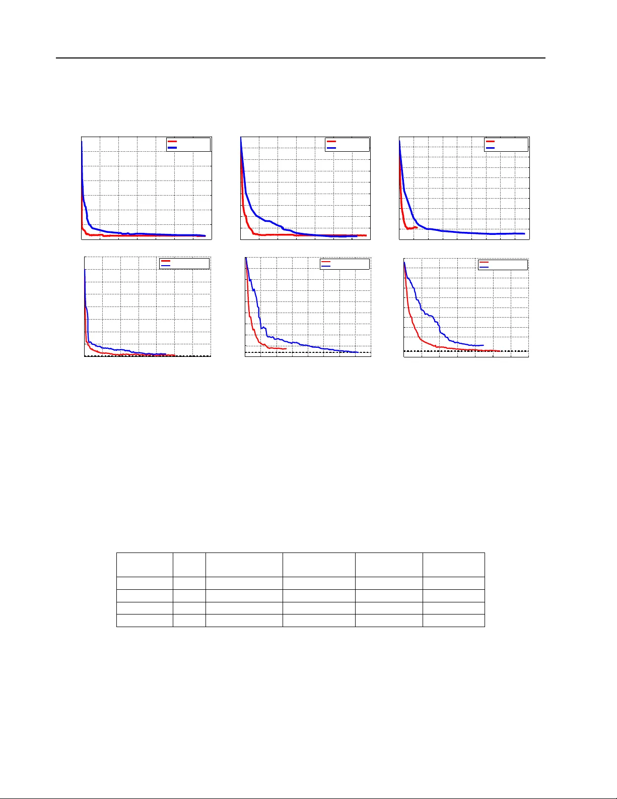
ShareBo ost: Efficien t Multiclass Learning with F eature Sharing Shai Shalev-Sh wartz shais@cs.huji.ac.il Sc ho ol of Computer Science and Engineering, the Hebrew Universit y of Jerusalem, Israel Y onatan W exler yona t an.wexler@orcam.com OrCam Ltd., Jerusalem, Israel Amnon Shash ua shashua@cs.huji.ac.il OrCam Ltd., Jerusalem, Israel Abstract Multiclass prediction is the problem of clas- sifying an ob ject into a relev an t target class. W e consider the problem of learning a mul- ticlass predictor that uses only few features, and in particular, the num b er of used features should increase sub-linearly with the num b er of p ossible classes. This implies that features should b e shared b y several classes. W e de- scrib e and analyze the ShareBo ost algorithm for learning a multiclass predictor that uses few shared features. W e prov e that Share- Bo ost efficiently finds a predictor that uses few shared features (if suc h a predictor ex- ists) and that it has a small generalization er- ror. W e also describ e ho w to use ShareBo ost for learning a non-linear predictor that has a fast ev aluation time. In a series of exp eri- men ts with natural data sets w e demonstrate the benefits of ShareBo ost and ev aluate its success relatively to other state-of-the-art ap- proac hes. 1. In tro duction Learning to classify an ob ject in to a relev an t target class surfaces in many domains suc h as do cumen t cate- gorization, ob ject recognition in computer vision, and w eb adv ertisement. In multiclass learning problems w e use training examples to learn a classifier which will later b e used for accurately classifying new ob- jects. T ypically , the classifier first calculates sev eral features from the input ob ject and then classifies the A short version of this man uscript will b e presented at NIPS, Dec. 2011. Part of this work was funded by ISF 519/09. A.S. is on sabbatical from the Hebrew Universit y . ob ject based on those features. In man y cases, it is im- p ortan t that the runtime of the learned classifier will b e small. In particular, this requires that the learned classifier will only rely on the v alue of few features. W e start with predictors that are based on line ar com- binations of features. Later, in Section 4 , w e sho w ho w our framework enables learning highly non-linear pre- dictors b y em b edding non-linearity in the construction of the features. Requiring the classifier to dep end on few features is therefore equiv alent to sparseness of the linear w eights of features. In recen t y ears, the problem of learning sparse v ectors for linear classification or re- gression has been given significant attention. While, in general, finding the most accurate sparse predic- tor is known to b e NP hard ( Natara jan , 1995 ; Davis et al. , 1997 ), t wo main approac hes ha ve b een prop osed for o vercoming the hardness result. The first approac h uses ` 1 norm as a surrogate for sparsity (e.g. the Lasso algorithm ( Tibshirani , 1996 ) and the compressed sens- ing literature ( Candes & T ao , 2005 ; Donoho , 2006 )). The second approac h relies on forw ard greedy selection of features (e.g. Bo osting ( F reund & Schapire , 1999 ) in the mac hine learning literature and orthogonal matc h- ing pursuit in the signal processing communit y ( T ropp & Gilb ert , 2007 )). A popular mo del for multiclass predictors maintains a w eight vector for each one of the classes. In such case, ev en if the w eigh t vector asso ciated with eac h class is sparse, the o verall n um b er of used features might gro w with the num b er of classes. Since the num b er of classes can be rather large, and our goal is to learn a mo del with an ov erall small n umber of features, we would like that the w eight v ectors will share the features with non-zero weigh ts as muc h as possible. Organizing the w eight vectors of all classes as rows of a single matrix, this is equiv alen t to requiring sparsit y of the c olumns of the matrix. ShareBo ost In this paper we describe and analyze an efficien t al- gorithm for learning a m ulticlass predictor whose cor- resp onding matrix of w eigh ts has a small n umber of non-zero columns. W e formally pro v e that if there exists an accurate matrix with a num b er of non-zero columns that grows sub-linearly with the n umber of classes, then our algorithm will also learn such a ma- trix. W e apply our algorithm to natural multiclass learning problems and demonstrate its adv an tages ov er previously prop osed state-of-the-art metho ds. Our algorithm is a generalization of the forw ard greedy selection approac h to sparsity in columns. An alter- nativ e approac h, whic h has recently b een studied in ( Quattoni et al. , 2009 ; Duchi & Singer , 2009 ), general- izes the ` 1 norm based approach, and relies on mixed- norms. W e discuss the adv an tages of the greedy ap- proac h ov er mixed-norms in Section 1.2 . 1.1. F ormal problem statemen t Let V b e the set of ob jects we w ould like to classify . F or example, V can b e the set of gray scale images of a certain size. F or each ob ject v ∈ V , we hav e a p ool of predefined d features, eac h of which is a real n umber in [ − 1 , 1]. That is, w e can represent eac h v ∈ V as a vector of features x ∈ [ − 1 , 1] d . W e note that the mapping from v to x can b e non-linear and that d can b e very large. F or example, we can define x so that each element x i corresp onds to some patc h, p ∈ {± 1 } q × q , and a threshold θ , where x i equals 1 if there is a patc h of v whose inner pro duct with p is higher than θ . W e discuss some generic metho ds for constructing features in Section 4 . F rom this p oin t on ward we assume that x is given. The set of p ossible classes is denoted b y Y = { 1 , . . . , k } . Our goal is to learn a m ulticlass predic- tor, which is a mapping from the features of an ob ject in to Y . W e focus on the set of predictors parametrized b y matrices W ∈ R k,d that tak es the following form: h W ( x ) = argmax y ∈Y ( W x ) y . (1) That is, the matrix W maps each d -dimensional fea- ture v ector into a k -dimensional score v ector, and the actual prediction is the index of the maximal element of the score vector. If the maximizer is not unique, we break ties arbitrarily . Recall that our goal is to find a matrix W with few non-zero columns. W e denote by W · ,i the i ’th column of W and use the notation k W k ∞ , 0 = |{ i : k W · ,i k ∞ > 0 }| to denote the n um b er of columns of W whic h are not iden tically the zero v ector. More generally , giv en a matrix W and a pair of norms k · k p , k · k r w e denote k W k p,r = k ( k W · , 1 k p , . . . , k W · ,d k p ) k r , that is, we apply the p -norm on the columns of W and the r -norm on the resulting d -dimensional v ector. The 0 − 1 loss of a multiclass predictor h W on an example ( x , y ) is defined as 1 [ h W ( x ) 6 = y ]. That is, the 0 − 1 loss equals 1 if h W ( x ) 6 = y and 0 otherwise. Since this loss function is not conv ex with respect to W , we use a surrogate con v ex loss f unction based on the follo wing easy to v erify inequalities: 1 [ h W ( x ) 6 = y ] ≤ 1 [ h W ( x ) 6 = y ] − ( W x ) y + ( W x ) h W ( x ) ≤ max y 0 ∈Y 1 [ y 0 6 = y ] − ( W x ) y + ( W x ) y 0 (2) ≤ ln X y 0 ∈Y e 1 [ y 0 6 = y ] − ( W x ) y +( W x ) y 0 . (3) W e use the notation ` ( W , ( x , y )) to denote the righ t- hand side (eqn. ( 3 )) of the abov e. The loss given in eqn. ( 2 ) is the m ulti-class hinge loss ( Crammer & Singer , 2003 ) used in Supp ort-V ector-Machines, whereas ` ( W , ( x , y )) is the result of performing a “soft- max” op eration: max x f ( x ) ≤ (1 /p ) ln P x e pf ( x ) , where equalit y holds for p → ∞ . This logistic multiclass loss function ` ( W, ( x , y )) has sev eral nice prop erties — see for example ( Zhang , 2004 ). Besides b eing a conv ex upper-b ound on the 0 − 1 loss, it is smo oth. The reason w e need the loss func- tion to b e b oth conv ex and smo oth is as follows. If a function is con vex, then its first order approximation at an y p oin t gives us a low er b ound on the function at any other p oin t. When the function is also smo oth, the first order appro ximation gives us b oth low er and upp er b ounds on the v alue of the function at any other p oin t 1 . ShareBoost uses the gradient of the loss func- tion at the curren t solution (i.e. the first order appro x- imation of the loss) to mak e a greedy choice of whic h column to update. T o ensure that this greedy choice indeed yields a significant impro vemen t we m ust know that the first order appro ximation is indeed close to the actual loss function, and for that we need b oth lo wer and upp er b ounds on the quality of the first or- der appro ximation. Giv en a training set S = ( x 1 , y 1 ) , . . . , ( x m , y m ), the a verage training loss of a matrix W is: L ( W ) = 1 m P ( x ,y ) ∈ S ` ( W , ( x , y )) . W e aim at approximately 1 Smo othness guaran tees that | f ( x ) − f ( x 0 ) − ∇ f ( x 0 )( x − x 0 ) | ≤ β k x − x 0 k 2 for some β and all x, x 0 . Therefore one can appro ximate f ( x ) b y f ( x 0 ) + ∇ f ( x 0 )( x − x 0 ) and the appro ximation error is upper b ounded b y the difference b et w een x, x 0 . ShareBo ost solving the problem min W ∈ R k,d L ( W ) s.t. k W k ∞ , 0 ≤ s . (4) That is, find the matrix W with minimal training loss among all matrices with column sparsity of at most s , where s is a user-defined parameter. Since ` ( W , ( x , y )) is an upp er b ound on 1 [ h W ( x ) 6 = y ], by minimizing L ( W ) w e also decrease the av erage 0 − 1 error of W o ver the training set. In Section 5 we show that for sparse mo dels, a small training error is lik ely to yield a small error on unseen examples as well. Regrettably , the constrain t k W k ∞ , 0 ≤ s in eqn. ( 4 ) is non-conv ex, and solving the optimization problem in eqn. ( 4 ) is NP-hard ( Natara jan , 1995 ; Davis et al. , 1997 ). T o ov ercome the hardness result, the Share- Bo ost algorithm will follo w the forward greedy selec- tion approach. The algorithm comes with formal gen- eralization and sparsity guarantees (describ ed in Sec- tion 5 ) that mak es ShareBoost an attractiv e m ulticlass learning engine due to efficiency (b oth during training and at test time) and accuracy . 1.2. Related W ork The cen trality of the m ulticlass learning problem has spurred the developmen t of v arious approac hes for tac kling the task. Perhaps the most straigh tforward approac h is a reduction from multiclass to binary , e.g. the one-vs-rest or all pairs constructions. The more direct approach w e choose, in particular, the multi- class predictors of the form giv en in eqn. ( 1 ), has b een extensiv ely studied and show ed a great success in prac- tice — see for example ( Duda & Hart , 1973 ; V apnik , 1998 ; Crammer & Singer , 2003 ). An alternativ e construction, abbreviated as the single- ve ctor mo del, shares a single weigh t vector, for all the classes, paired with class-sp ecific feature mappings. This construction is common in generalized additive mo dels ( Hastie & Tibshirani , 1995 ), m ulticlass ver- sions of bo osting ( F reund & Sc hapire , 1997 ; Schapire & Singer , 1999 ), and has been p opularized lately due to its role in prediction with structured output where the num ber of classes is exp onentially large (see e.g. ( T ask ar et al. , 2003 )). While this approach can yield predictors with a rather mild dep endency of the re- quired features on k (see for example the analysis in ( Zhang , 2004 ; T ask ar et al. , 2003 ; Fink et al. , 2006 )), it relies on a-priori assumptions on the structure of X and Y . In contrast, in this pap er w e tac kle general m ulticlass prediction problems, like ob ject recognition or do cumen t classification, where it is not straigh t- forw ard or even plausible ho w one would go about to construct a-priori goo d class sp ecific feature mappings, and therefore the single-vector mo del is not adequate. The class of predictors of the form given in eqn. ( 1 ) can b e trained using F rob enius norm regularization (as done by m ulticlass SVM – see e.g. ( Crammer & Singer , 2003 )) or using ` 1 regularization o ver all the entries of W . Ho wev er, as pointed out in ( Quattoni et al. , 2009 ), these regularizers migh t yield a matrix with man y non- zeros columns, and hence, will lead to a predictor that uses man y features. The alternative approach, and the most relev ant to our work, is the use of mix-norm regularizations like k W k ∞ , 1 or k W k 2 , 1 ( Lanc kriet et al. , 2004 ; T urlach et al. , 2000 ; Argyriou et al. , 2006 ; Bac h , 2008 ; Quattoni et al. , 2009 ; Duchi & Singer , 2009 ; Huang & Zhang , 2010 ). F or example, ( Duchi & Singer , 2009 ) solves the follo wing problem: min W ∈ R k,d L ( W ) + λ k W k ∞ , 1 . (5) whic h can b e view ed as a con vex appro ximation of our ob jective (eqn. ( 4 )). This is adv an tageous from an op- timization p oin t of view, as one can find the global optim um of a conv ex problem, but it remains unclear ho w well the conv ex program approximates the orig- inal goal. F or example, in Section 6 we sho w cases where mix-norm regularization does not yield sparse solutions while ShareBoost do es yield a sparse solu- tion. Despite the fact that ShareBo ost tackles a non- con vex program, and thus limited to local optimum solutions, we pro ve in Theorem 2 that under mild con- ditions ShareBo ost is guar ante e d to find an accurate sparse solution whenever such a solution exists and that the generalization error is b ounded as shown in Theorem 1 . W e note that several recent papers (e.g. ( Huang & Zhang , 2010 )) established exact recov ery guaran tees for mixed norms, whic h may seem to b e stronger than our guarantee given in Theorem 2 . Ho wev er, the assumptions in ( Huang & Zhang , 2010 ) are muc h stronger than the assumptions of Theorem 2 . In particular, they hav e strong noise assumptions and a group RIP like assumption (Assumption 4.1-4.3 in their pap er). In contrast, w e imp ose no such restric- tions. W e would lik e to stress that in many generic practical cases, the assumptions of ( Huang & Zhang , 2010 ) will not hold. F or example, when using decision stumps, features will be highly correlated whic h will violate Assumption 4.3 of ( Huang & Zhang , 2010 ). Another adv antage of ShareBo ost is that its only pa- rameter is the desired num b er of non-zero columns of W . F urthermore, obtaining the whole-regularization- path of ShareBoost, that is, the curv e of accuracy as a function of sparsity , can b e p erformed by a single run ShareBo ost of ShareBo ost, which is muc h easier than obtaining the whole regularization path of the conv ex relaxation in eqn. ( 5 ). Last but not least, ShareBoost can w ork ev en when the initial num b er of features, d , is very large, as long as there is an efficient wa y to choose the next feature. F or example, when the features are con- structed using decision stumps, d will b e extremely large, but ShareBo ost can still b e implemen ted effi- cien tly . In con trast, when d is extremely large mix- norm regularization techniques yield challenging opti- mization problems. As men tioned before, ShareBo ost follo ws the forward greedy selection approach for tac kling the hardness of solving eqn. ( 4 ). The greedy approac h has been widely studied in the context of learning sparse predictors for linear regression. How ever, in m ulticlass problems, one needs sparsity of groups of v ariables (columns of W ). ShareBoost generalizes the fully corrective greedy selection pro cedure given in ( Shalev-Shw artz et al. , 2010 ) to the case of selection of groups of v ariables, and our analysis follo ws similar techniques. Obtaining group sparsity by greedy metho ds has b een also recen tly studied in ( Huang et al. , 2009 ; Ma jumdar & W ard , 2009 ), and indeed, ShareBoost shares simi- larities with these w orks. W e differ from ( Huang et al. , 2009 ) in that our analysis do es not impose strong as- sumptions (e.g. group-RIP) and so ShareBo ost applies to a m uc h wider arra y of applications. In addition, the sp ecific criterion for c ho osing the next feature is differ- en t. In ( Huang et al. , 2009 ), a ratio b et ween difference in ob jective and different in costs is used. In Share- Bo ost, the L1 norm of the gradien t matrix is used. F or the multiclass problem with log loss, the criterion of ShareBoost is muc h easier to compute, esp ecially in large scale problems. ( Ma jumdar & W ard , 2009 ) suggested many other selection rules that are geared to ward the squared loss, which is far from being an optimal loss function for m ulticlass problems. Another related method is the JointBoost algorithm ( T orralba et al. , 2007 ). While the original presen tation in ( T orralba et al. , 2007 ) seems rather differen t than the t yp e of predictors w e describe in eqn. ( 1 ), it is p os- sible to sho w that JointBoost in fact learns a matrix W with additional constrain ts. In particular, the features x are assumed to b e decision stumps and eac h column W · ,i is constrained to b e α i ( 1 [1 ∈ C i ] , . . . , 1 [ k ∈ C i ]), where α i ∈ R and C i ⊂ Y . That is, the stump is shared b y all classes in the subset C i . Join tBo ost chooses suc h shared decision stumps in a greedy manner b y apply- ing the GentleBoost algorithm on top of this presen ta- tion. A ma jor disadv an tage of JointBoost is that in its pure form, it should exhaustively search C among all 2 k p ossible subsets of Y . In practice, ( T orralba et al. , 2007 ) relies on heuristics for finding C on each b o ost- ing step. In con trast, ShareBo ost allo ws the columns of W to b e any real num bers, thus allo wing ”soft” sharing b et ween classes. Therefore, ShareBo ost has the same (or even richer) expressive p o wer comparing to JointBoost. Moreo ver, ShareBo ost automatically iden tifies the relatedness b et ween classes (corresp ond- ing to choosing the set C ) without ha ving to rely on exhaustiv e search. ShareBo ost is also fully corrective, in the sense that it extracts all the information from the selected features b efore adding new ones. This leads to higher accuracy while using less features as w as shown in our exp erimen ts on image clas sification. Lastly , ShareBo ost comes with theoretical guaran tees. Finally , we mention that feature sharing is merely one w ay for transferring information across classes ( Thrun , 1996 ) and sev eral alternative wa ys ha ve b een proposed in the literature such as target embedding ( Hsu et al. , 2010 ; Bengio et al. , 2011 ), shared hidden structure ( Le- Cun et al. , 1998 ; Amit et al. , 2007 ), shared prototypes ( Quattoni et al. , 2008 ), or sharing underlying metric ( Xing et al. , 2003 ). 2. The ShareBoost Algorithm ShareBo ost is a forward greedy selection approach for solving eqn. ( 4 ). Usually , in a greedy approac h, we up- date the w eight of one feature at a time. No w, we will up date one column of W at a time (since the desired sparsit y is ov er columns). W e will c ho ose the column that maximizes the ` 1 norm of the corresponding col- umn of the gradien t of the loss at W . Since W is a matrix w e hav e that ∇ L ( W ) is a matrix of the partial deriv ativ es of L . Denote by ∇ r L ( W ) the r ’th column of ∇ L ( W ), that is, the vector  ∂ L ( W ) ∂ W 1 ,r , . . . , ∂ L ( W ) ∂ W k,r  . A standard calculation sho ws that ∂ L ( W ) ∂ W q ,r = 1 m X ( x ,y ) ∈ S X c ∈Y ρ c ( x , y ) x r ( 1 [ q = c ] − 1 [ q = y ]) where ρ c ( x , y ) = e 1 [ c 6 = y ] − ( W x ) y +( W x ) c P y 0 ∈Y e 1 [ y 0 6 = y ] − ( W x ) y +( W x ) y 0 . (6) Note that P c ρ c ( x , y ) = 1 for all ( x , y ). Therefore, we can rewrite, ∂ L ( W ) ∂ W q ,r = 1 m X ( x ,y ) x r ( ρ q ( x , y ) − 1 [ q = y ]) . ShareBo ost Based on the ab o v e we hav e k∇ r L ( W ) k 1 = 1 m X q ∈Y       X ( x ,y ) x r ( ρ q ( x , y ) − 1 [ q = y ])       . (7) Finally , after choosing the column for which k∇ r L ( W ) k 1 is maximized, w e re-optimize all the columns of W whic h were selected so far. The re- sulting algorithm is giv en in Algorithm 1 . Algorithm 1 ShareBo ost 1: Initialize: W = 0 ; I = ∅ 2: for t=1,2,. . . ,T do 3: F or eac h class c and example ( x , y ) define ρ c ( x , y ) as in eqn. ( 6 ) 4: Cho ose feature r that maximizes the right-hand side of eqn. ( 7 ) 5: I ← I ∪ { r } 6: Set W ← argmin W L ( W ) s.t. W · ,i = 0 for all i / ∈ I 7: end for The runtime of ShareBo ost is as follows. Steps 3-5 requires O ( mdk ). Step 6 is a conv ex optimization problem in tk v ariables and can be performed using v arious metho ds. In our exp erimen ts, we used Nes- tero v’s accelerated gradient method ( Nesterov & Nes- tero v , 2004 ) whose run time is O ( mtk / √  ) for a smooth ob jective, where  is the desired accuracy . Therefore, the ov erall runtime is O ( T mdk + T 2 mk / √  ). It is in- teresting to compare this runtime to the complexity of minimizing the mixed-norm regularization ob jec- tiv e given in eqn. ( 5 ). Since the ob jectiv e is no longer smo oth, the runtime of using Nestero v’s accelerated metho d w ould b e O ( mdk / ) which can be muc h larger than the run time of ShareBo ost when d  T . 3. V ariants of ShareBo ost W e no w describ e sev eral v ariants of ShareBoost. The analysis we present in Section 5 can b e easily adapted for these v arian ts as well. 3.1. Mo difying the Greedy Choice Rule ShareBo ost c ho oses the feature r which maximizes the ` 1 norm of the r -th column of the gradien t matrix. Our analysis shows that this choice leads to a sufficien t decrease of the ob jective function. Ho wev er, one can easily dev elop other wa ys for choosing a feature which ma y p oten tially lead to an even larger decrease of the ob jective. F or example, we can choose a feature r that minimizes L ( W ) o ver matrices W with supp ort of I ∪ { r } . This will lead to the maximal p ossible decrease of the ob jective function at the curren t iteration. Of course, the run time of choosing r will no w b e muc h larger. Some intermediate options are to c ho ose r that minimizes min α ∈ R W + α ∇ r R ( W ) or to c ho ose r that minimizes min w ∈ R k W + w e † r , where e † r is the all-zero row vector except 1 in the r ’th p osition. 3.2. Selecting a Group of F eatures at a Time In some situations, features can b e divided into groups where the run time of calculating a single feature in eac h group is almost the same as the runtime of cal- culating all features in the group. In such cases, it mak es sense to choose groups of features at each iter- ation of ShareBoost. This can be easily done b y sim- ply choosing the group of features J that maximizes P j ∈ J k∇ j L ( W ) k 1 . 3.3. Adding Regularization Our analysis implies that when | S | is significantly larger than ˜ O ( T k ) then ShareBo ost will not o v erfit. When this is not the case, we can incorp orate reg- ularization in the ob jective of ShareBo ost in order to preven t o verfitting. One simple w ay is to add to the ob jectiv e function L ( W ) a F rob enius norm reg- ularization term of the form λ P i,j W 2 i,j , where λ is a regularization parameter. It is easy to v erify that this is a smo oth and con vex function and therefore we can easily adapt ShareBoost to deal with this regu- larized ob jective. It is also p ossible to rely on other norms such as the ` 1 norm or the ` ∞ /` 1 mixed-norm. Ho wev er, there is one technicalit y due to the fact that these norms are not smooth. W e can o vercome this problem by defining smo oth approximations to these norms. The main idea is to first note that for a scalar a w e ha ve | a | = max { a, − a } and therefore w e can rewrite the aforementioned norms using max and sum operations. Then, we can replace eac h max expression with its soft-max coun terpart and obtain a smo oth v ersion of the ov erall norm function. F or example, a smo oth version of the ` ∞ /` 1 norm will b e k W k ∞ , 1 ≈ 1 β P d j =1 log  P k i =1 ( e β W i,j + e − β W i,j )  , where β ≥ 1 controls the tradeoff b etw een qualit y of appro ximation and smo othness. ShareBo ost 0 0.5 1 1.5 2 2.5 3 3.5 4 4.5 5 0 0.2 0.4 0.6 0.8 1 1.2 1.4 1.6 1.8 2 Figure 1. Motiv ating sup er vectors. 4. Non-Linear Prediction Rules W e now demonstrate ho w ShareBo ost can b e used for learning non-linear predictors. The main idea is similar to the approac h tak en b y Boosting and SVM. That is, we construct a non-linear predictor by first mapping the original features into a higher dimen- sional space and then learning a linear predictor in that space, which corresponds to a non-linear predic- tor ov er the original feature space. T o illustrate this idea we present tw o concrete mappings. The first is the decision stumps metho d whic h is widely used by Bo osting algorithms. The second approach sho ws ho w to use ShareBoost for learning piece-wise linear predic- tors and is inspired b y the sup er-v ectors construction recen tly describ ed in ( Zhou et al. , 2010 ). 4.1. ShareBo ost with Decision Stumps Let v ∈ R p b e the original feature v ector represent- ing an ob ject. A decision stump is a binary feature of the form 1 [ v i ≤ θ ], for some feature i ∈ { 1 , . . . , p } and threshold θ ∈ R . T o construct a non-linear predic- tor w e can map each ob ject v in to a feature-vector x that con tains all p ossible decision stumps. Naturally , the dimensionality of x is very large (in fact, can even b e infinite), and calculating Step 4 of ShareBo ost may tak e forever. Luc kily , a simple trick yields an efficient solution. First note that for each i , all stump features corresp onding to i can get at most m + 1 v alues on a training set of size m . Therefore, if we sort the v alues of v i o ver the m examples in the training set, w e can calculate the v alue of the right-hand side of eqn. ( 7 ) for all p ossible v alues of θ in total time of O ( m ). Thus, ShareBo ost can b e implemen ted efficien tly with deci- sion stumps. 4.2. Learning Piece-wise Linear Predictors with ShareBo ost T o motiv ate our next construction let us consider first a simple one dimensional function estimation problem. Giv en sample ( x 1 , y i ) , . . . , ( x m , y m ) w e would like to find a function f : R → R such that f ( x i ) ≈ y i for all i . The class of piece-wise linear functions can b e a go od candidate for the approximation function f . See for example an illustration in Fig. 1 . In fact, it is easy to verify that all smooth functions can b e approx- imated by piece-wise linear functions (see for example the discussion in ( Zhou et al. , 2010 )). In general, w e can express piece-wise linear vector-v alued functions as f ( v ) = q X j =1 1 [ k v − v j k < r j ] ( h u j , v i + b j ) , where q is the num b er of pieces, ( u j , b j ) represents the linear function corresp onding to piece j , and ( v j , r j ) represen ts the center and radius of piece j . This ex- pression can be also written as a linear function o ver a differen t domain, f ( v ) = h w , ψ ( v ) i where ψ ( v ) = [ 1 [ k v − v 1 k < r 1 ] [ v , 1] , . . . , 1 [ k v − v q k < r q ] [ v , 1] ] . In the case of learning a multiclass predictor, we shall learn a predictor v 7→ W ψ ( v ), where W will b e a k by dim( ψ ( v )) matrix. ShareBoost can b e used for learning W . F urthermore, w e can apply the v ariant of ShareBo ost described in Section 3.2 to learn a piece- wise linear model whic h few pieces (that is, each group of features will corresp ond to one piece of the mo del). In practice, we first define a large set of candidate cen- ters by applying some clustering metho d to the train- ing examples, and second we define a set of p ossible radiuses by taking v alues of quan tiles from the training examples. Then, w e train ShareBo ost so as to c ho ose a multiclass predictor that only use few pairs ( v j , r j ). The adv antage of using ShareBo ost here is that while it learns a non-linear mo del it will try to find a mo del with few linear “pieces”, whic h is adv antageous both in terms of test runtime as well as in terms of gener- alization p erformance. 5. Analysis In this section w e provide formal guaran tees for the ShareBo ost algorithm. The pro ofs are deferred to the app endix. W e first show that if the algorithm has managed to find a matrix W with a small num b er of non-zero columns and a small training error, then the generalization error of W is also small. The b ound b elo w is in terms of the 0 − 1 loss. A related bound, whic h is given in terms of the conv ex loss function, is describ ed in ( Zhang , 2004 ). Theorem 1 Supp ose that the Shar eBo ost algorithm runs for T iter ations and let W b e its output matrix. Then, with pr ob ability of at le ast 1 − δ over the choic e ShareBo ost of the tr aining set S we have that P ( x ,y ) ∼D [ h W ( x ) 6 = y ] ≤ P ( x ,y ) ∼ S [ h W ( x ) 6 = y ] + O s T k log ( T k ) log ( k ) + T log ( d ) + log(1 /δ ) | S | ! Next, w e analyze the sparsity guarantees of Share- Bo ost. As mentioned previously , exactly solving eqn. ( 4 ) is known to b e NP hard. The following main theorem giv es an in teresting appro ximation guaran tee. It tells us that if there exists an accurate solution with small ` ∞ , 1 norm, then the ShareBo ost algorithm will find a go od sparse solution. Theorem 2 L et  > 0 and let W ? b e an arbitr ary ma- trix. Assume that we run the Shar eBo ost algorithm for T =  4 1  k W ? k 2 ∞ , 1  iter ations and let W b e the output matrix. Then, k W k ∞ , 0 ≤ T and L ( W ) ≤ L ( W ? ) +  . 6. F eature Sharing — Illustrativ e Examples In this section we present illustrative examples, show- ing that whenever strong feature sharing is p ossible then ShareBo ost will find it, while comp etitive meth- o ds migh t fail to pro duce solutions with a small num- b er of features. In the analysis of the examples b elo w we use the fol- lo wing simple corollary of Theorem 2 . Corollary 1 Assume that ther e exists a matrix W ? such that L ( W ? ) ≤  , al l entries of W ? ar e in [ − c, c ] , and k W ? k ∞ , 0 = r . Then, Shar eBo ost wil l find a ma- trix W with L ( W ) ≤ 2  and k W k ∞ , 0 ≤ 4 r 2 c 2 / . The first example we present shows an exp onential gap b et w een the num b er of features required by Share- Bo ost (as well as mixed norms) and the num b er of features required by ` 2 or ` 1 regularization metho ds. Consider a set of examples suc h that eac h exam- ple, ( x , y ), is of the form x = [bin( y ) , 2 log ( k ) e y ] ∈ R log( k )+ k , where bin( y ) ∈ {± 1 } log( k ) is the binary rep- resen tation of the num b er y in the alphabet {± 1 } and e y is the vector which is zero everywhere except 1 in the y ’th coordinate. F or example, if k = 4 then bin(1) = [ − 1 , 1], bin(2) = [1 , − 1], bin(3) = [1 , 1], and bin(4) = [ − 1 , − 1]. Consider tw o matrices. The first matrix, de- noted W ( s ) , is the matrix whose row y equals to [bin( y ) , (0 , . . . , 0)]. The second matrix, denoted W ( f ) , is the matrix whose row y equals to [(0 , . . . , 0) , e y ]. Clearly , the num b er of features used b y h W ( s ) is log( k ) while the n umber of features used by h W ( f ) is k . Observ e that b oth h W ( f ) ( x ) and h W ( s ) ( x ) (see defi- nition in eqn. ( 1 )), will make perfect predictions on the training set. F urthermore, since for eac h exam- ple ( x , y ), for each r 6 = y we hav e that ( W ( s ) x ) r ∈ [ − log ( k ) , log ( k ) − 2], for the logistic multiclass loss, for an y c > 0 we hav e that L ( cW ( f ) ) = log(1 + ( k − 1) e 1 − 2 c log( k ) ) < L ( cW ( s ) ) < log(1 + ( k − 1) e 1 − c (log( k ) − 2) ) . It follo ws that for c ≥ 1 + log ( k − 1) − log( e  − 1) log( k ) − 2 w e hav e that L ( cW ( s ) ) ≤  . Consider an algorithm that solves the regularized problem min W L ( W ) + λ k W k p,p , where p is either 1 or 2. In b oth cases, w e ha v e that 2 k W ( f ) k p,p < k W ( s ) k p,p . It follo ws that for any v alue of λ , and for an y c > 0, the v alue of the ob jective at cW ( f ) is smaller than the v alue at cW ( s ) . In fact, it is not hard to sho w that the optimal solution takes the form cW ( f ) for some c > 0. Therefore, no matter what the regularization parameter λ is, the solution of the abov e regularized problem will use k features, even though there exists a rather go od solution that relies on log( k ) shared features. In con trast, using Corollary 1 we know that if we stop ShareBo ost after p oly(log( k )) iterations it will pro- duce a matrix that uses only p oly(log ( k )) features and has a small loss. Similarly , it is possible to sho w that for an appropriate regularization parameter, the mix- norm regularization k W k ∞ , 1 will also yield the matrix W ( s ) rather than the matrix W ( f ) . In our second example we show that in some situations using the mix-norm regularization, min W L ( W ) + λ k W k ∞ , 1 , will also fail to produce a sparse solution, while Share- Bo ost is still guaranteed to learn a sparse solution. Let s b e an integer and consider examples ( x , y ) where eac h x is comp osed of s blocks, each of which is in {± 1 } log( k ) . W e consider tw o types of examples. In the first type, each block of x equals to bin( y ). In the second type, w e generate example as in the first t yp e, but then w e zero one of the blo c ks (where we 2 k W ( f ) k p p,p = k whereas k W ( s ) k p p,p = k log( k ). ShareBo ost c ho ose uniformly at random which blo c k to zero). As b efore, (1 −  ) m examples are of the first type while m examples are of the second t yp e. Consider again t wo matrices. The first matrix, denoted W ( s ) , is the matrix whose row y equals to [bin( y ) , (0 , . . . , 0)]. The second matrix, de- noted W ( f ) , is the matrix whose ro w y equals to [bin( y ) , . . . , bin( y )] /s . Note that k W ( f ) k ∞ , 1 = k W ( s ) k ∞ , 1 . In addition, for any ( x , y ) of the second t yp e we hav e that E [ W ( s ) x ] = W ( f ) x , where exp ecta- tion is with resp ect to the choice of whic h block to zero. Since the loss function is strictly conv ex, it follows from Jensen’s inequality that L ( W ( f ) ) < L ( W ( s ) ). W e ha ve thus shown that using the ( ∞ , 1) mix-norm as a regularization will prefer the matrix W ( f ) o ver W ( s ) . In fact, it is possible to sho w that the minimizer of L ( W ) + λ k W k ∞ , 1 will b e of the form cW ( f ) for some c . Since the num b er of blo c ks, s , was arbitrarily large, and since ShareBoost is guaranteed to learn a matrix with at most p oly(log( k )) non-zero columns, we con- clude that there can b e a substantial gap betw een mix- norm regularization and ShareBo ost. The adv antage of ShareBo ost in this example follows from its ability to break ties (ev en in an arbitrary wa y). Naturally , the aforementioned examples are synthetic and capture extreme situations. How ever, in our ex- p erimen ts b elo w we sho w that ShareBo ost p erforms b etter than mixed-norm regularization on natural data sets as w ell. 7. Exp erimen ts In this section we demonstrate the merits (and pitfalls) of ShareBo ost by comparing it to alternative algo- rithms in different scenarios. The first exp eriment ex- emplifies the feature sharing prop ert y of ShareBo ost. W e p erform exp erimen ts with an OCR data set and demonstrate a mild gro wth of the num b er of features as the num b er of classes gro ws from 2 to 36. The sec- ond experiment compares ShareBo ost to mixed-norm regularization and to the Join tBo ost algorithm of ( T or- ralba et al. , 2007 ). W e follow the same experimental setup as in ( Duchi & Singer , 2009 ). The main finding is that ShareBo ost outp erforms the mixed-norm regu- larization metho d when the output predictor needs to b e v ery sparse, while mixed-norm regularization can b e b etter in the regime of rather dense predictors. W e also show that ShareBo ost is b oth faster and more ac- curate than JointBoost. The third and final set of ex- p erimen ts is on the MNIST handwritten digit dataset where we demonstrate state-of-the-art accuracy at ex- tremely efficien t runtime p erformance. 0 5 10 15 20 25 30 35 40 0 50 100 150 200 250 300 350 # classes # features Figure 2. The num b er of features required to achiev e a fixed accuracy as a function of the num b er of classes for ShareBo ost (dashed) and the 1-vs-rest (solid-circles). The blue lines are for a target error of 20% and the green lines are for 8%. 7.1. F eature Sharing The main motiv ation for deriving the ShareBo ost algo- rithm is the need for a multiclass predictor that uses only few features, and in particular, the num b er of features should increase slo wly with the num b er of classes. T o demonstrate this prop ert y of ShareBo ost w e experimented with the Char74k data set whic h con- sists of images of digits and letters. W e trained Share- Bo ost with the num b er of classes v arying from 2 classes to the 36 classes corresp onding to the 10 digits and 26 capital letters. W e calculated how many features were required to ac hieve a certain fixed accuracy as a func- tion of the n umber of classes. The description of the feature space is describ ed in Section 7.4 . W e compared ShareBoost to the 1-vs-rest approach, where in the latter, w e trained eac h binary classifier using the same mechanism as used by ShareBo ost. Namely , we minimize the binary logistic loss using a greedy algorithm. Both methods aim at constructing sparse predictors using the same greedy approach. The difference b etw een the metho ds is that ShareBo ost se- lects features in a shared manner while the 1-vs-rest approac h selects features for each binary problem sep- arately . In Fig. 2 we plot the ov erall n umber of features required by b oth metho ds to achiev e a fixed accuracy on the test set as a function of the n umber of classes. As can b e easily seen, the increase in the n umber of required features is mild for ShareBoost but significant for the 1-vs-rest approac h. 7.2. Comparing ShareBo ost to Mixed-Norms Regularization Our next exp erimen t compares ShareBo ost to the use of mixed-norm regularization (see eqn. ( 5 )) as a surro- ShareBo ost gate for the non-conv ex sparsity constrain t. See Sec- tion 1.2 for description of the approac h. T o make the comparison fair, w e follow ed the same exp erimen tal setup as in ( Duchi & Singer , 2009 ) (using co de pro- vided b y ). W e calculated the whole regularization path for the mixed-norm regularization b y running the algorithm of ( Duc hi & Singer , 2009 ) with many v alues of the regularization parameter λ . In Fig. 3 we plot the re- sults on three UCI datasets: StatLog, Pendigits and Isolet. The n umber of classes for the datasets are 7,10,26, resp ectiv ely . The original dimensionalit y of these datasets is not very high and therefore, follo w- ing ( Duchi & Singer , 2009 ), we expanded the features b y taking all products o ver ordered pairs of features. After this transformation, the n umber of features w ere 630, 120, 190036, resp ectiv ely . Fig. 3 displays the results. As can b e seen, Share- Bo ost decreases the error muc h faster than the mixed- norm regularization, and therefore is preferable when the goal is to hav e a rather sparse solution. When more features are allo wed, ShareBo ost starts to ov erfit. This is not surprising since here sparsit y is our only mean for controlling the complexity of the learned classifier. T o prev ent this ov erfitting effect, one can use the v ari- an t of ShareBo ost that incorp orates regularization— see Section 3 . 7.3. Comparing ShareBo ost to Join tBo ost Here w e compare ShareBo ost to the Join tBo ost algo- rithm of ( T orralba et al. , 2007 ). See Section 1.2 for description of Join tBo ost. As in the previous exp eri- men t, we follo w ed the exp erimen tal setup as in ( Duchi & Singer , 2009 ) and ran JointBoost of ( T orralba et al. , 2007 ) using their published code with additional im- plemen tation of the BFS heuristic for pruning the 2 k space of all class-subsets as describ ed in their pap er. Fig. 3 (b ottom) displays the results. Here we used stump features for b oth algorithms since these are needed for Join tBo ost. As can be seen, ShareBo ost decreases the error m uch faster and therefore is prefer- able when the goal is to hav e a rather sparse solution. As in the previous exp erimen t we observ e that when more features are allow ed, ShareBo ost starts to o ver- fit. Again, this is not surprising and can b e preven ted b y adding additional regularization. The training run- time of ShareBoost is also m uch shorter than that of Join tBo ost (see discussion in Section 1.2 ). 7.4. MNIST Handwritten Digits Dataset The goal of this exp eriment is to show that ShareBoost ac hieves state-of-the-art p erformance while construct- ing v ery fast predictors. W e exp erimen ted with the MNIST digit dataset, which consists of a training set of 60 , 000 digits represented by centered size-normalized 28 × 28 images, and a test set of 10 , 000 digits (see Fig. 6 for some examples). The MNIST datase t has b een extensively studied and is considered the stan- dard test for multiclass classification of handwritten digits. The error rate achiev ed b y the most adv anced algorithms are below 1% of the test set (i.e., below 100 classification mistakes on the test set). T o get a sense of the challenge inv olved with the MNIST dataset, con- sider a straightforw ard 3-Nearest-Neighbor (3NN) ap- proac h where each test example x , represented as a v ector with 28 2 en tries, is matc hed against the entire training set x j using the distance d ( x , x j ) = k x − x j k 2 . The classification decision is then the ma jorit y class la- b el of the three most nearest training examples. This naiv e 3NN approach achiev es an error rate of 2 . 67% (i.e., 267 mis-classification errors) with a run-time of un wieldy prop ortions. Going from 3NN to qNN with q = 4 , ..., 12 do es not pro duce a b etter error rate. More adv anced shap e-similarit y measures could im- pro ve the p erformance of the naive q N N approac h but at a hea vier run-time cost. F or example, the Shap e Context similarity measure introduced b y ( Be- longie et al. , 2002 ) uses a Bipartite matching algo- rithm b etw een descriptors computed along 100 p oin ts in each image. A 3NN using Shap e-Context similar- it y ac hiev es an error rate of 0 . 63% but at a very high (practically unwieldy) run-time cost. The challenge with the MNIST dataset is, therefore, to design a m ul- ticlass algorithm with a small error rate (say b elo w 1%) and hav e an efficient run-time p erformance. The top MNIST p erformer ( Ciresan et al. , 2010 ) uses a feed-forw ard Neural-Net with 7 . 6 million connec- tions whic h roughly translates to 7 . 6 million m ultiply- accum ulate (MAC) op erations at run-time as well. During training, geometrically distorted versions of the original examples w ere generated in order to expand the training set following ( Simard et al. , 2003 ) who in- tro duced a warping scheme for that purp ose. The top p erformance error rate stands at 0 . 35% at a run-time cost of 7 . 6 million MA C p er test example. T able 1 summarizes the discussion so far including the p erformance of ShareBo ost. The error-rate of ShareBo ost with 266 rounds stands on 0 . 71% using the original training set and 0 . 47% with the expanded training set of 360 , 000 examples generated by adding fiv e deformed instances p er original example and with ShareBo ost 0 100 200 300 400 500 600 700 0.1 0.2 0.3 0.4 0.5 0.6 0.7 0.8 Proportion of used features Test Error ShareBoost Mixed−norms 0 20 40 60 80 100 120 140 0 0.1 0.2 0.3 0.4 0.5 0.6 0.7 0.8 0.9 Test Error Proportion of used features ShareBoost Mixed−norms 0 50 100 150 200 250 300 350 400 450 0 0.1 0.2 0.3 0.4 0.5 0.6 0.7 0.8 0.9 1 Proportion of used features Test Error ShareBoost Mixed−norms 0 0.05 0.1 0.15 0.2 0.25 0.3 0.35 0.107 0.2 0.3 0.4 0.5 0.6 0.7 0.8 0.9 Proportion of used features Test error ShareBoost − stumps JointBoost 0 0.1 0.2 0.3 0.4 0.5 0.6 0.7 0.8 0.0383 0.1 0.2 0.3 0.4 0.5 0.6 0.7 0.8 0.9 Proportion of used features Test error ShareBoost − stumps JointBoost 0 0.05 0.1 0.15 0.2 0.25 0.3 0.35 0 0.0564 0.2 0.3 0.4 0.5 0.6 0.7 0.8 0.9 1 Proportion of used features Test error ShareBoost − stumps JointBoost (a) StatLog (b) P endigits (c) Isolet Figure 3. ShareBo ost compared with mixed-norm regularization (top) and JointBoost (b ottom) on several UCI datasets. The horizontal axis is the feature sparsity (fraction of features used) and the vertical axis is the test error rate. Reference 3NN Shap e Context SVM 9-p oly Neural Net ShareBo ost Belongie-et-al DeCosta-et-al Ciresan-et-al Error rate 2.7% 0.63% 0.56% 0.35% 0.47% Errors 270 63 56 35 47 Y ear – 2002 2002 2010 2011 Run time × 14 × 1000’s × 38 × 2.5 1 T able 1. Comparison of ShareBoost and relev ant metho ds on error rate and computational complexity ov er the MNIST dataset. More details in the text. ShareBo ost T = 305 rounds. The run-time on test examples is around 40% of the leading MNIST p erformer. The er- ror rate of 0 . 47% is b etter than that rep orted by ( De- coste & Bernhard , 2002 ) who used a 1-vs-all SVM with a 9-degree polynomial kernel and with an expanded training set of 780 , 000 examples. The num b er of sup- p ort v ectors (accumulated o ver the ten separate bi- nary classifiers) was 163 , 410 giving rise to a run-time of 21-fold compared to ShareBo ost. W e describe below the details of the ShareBo ost implementation on the MNIST dataset. The feature space w e designed consists of 7 × 7 image patc hes with corresponding spatial masks, constructed as follows. All 7 × 7 patches were collected from all images and clustered using K-means to produce 1000 cen ters w f . F or each such center (patc h) we also asso- ciated a set of 16 p ossible masks g f in order to limit the spatial lo cations of the maximal response of the 7 × 7 patc h. The pairs F = { ( v f , g f ) } form the p ool of d = 16 , 000 templates (shap e plus location). The v ec- tor of feature measurements x ∈ R m = ( . . . , x f c , . . . ) has each of its entries asso ciated with one of the tem- plates where an entry x f c = max n ( I ⊗ w f ) × g c f o . That is, a feature is the maximal resp onse of the con- v olution of the template w f o ver the image, w eighted b y the Gaussian g c f . ShareBo ost selects a subset of the templates j 1 , . . . , j T where eac h j i represen ts some template pair ( w f i , g c i f i ), and the matrix W ∈ R k × T . A test image I is then con- v erted to ˜ x ∈ R T using ˜ x i = max { ( I ⊗ w f i ) × g c i f i } with the maximum going o v er the image locations. The pre- diction ˆ y is then argmax y ∈ [ k ] ( W ˜ x ) y . Fig. 5 (a) shows the first 30 templates that were chosen by ShareBo ost and their corresp onding spatial masks. F or example, the first templates matc hes a digit part along the top of the image, the eleven th template matc hes a hori- zon tal stroke near the top of the image and so forth. Fig. 5 (b) sho ws the weigh ts (columns of W ) of the first 30 templates of the mo del that pro duced the b est results. F or example, the eleven th template which en- co des a horizon tal line close to the top is exp ected in the digit “9” but not in the digit “4”. Fig. 6 shows the 47 misclassified samples after T = 305 rounds of ShareBo ost, and Fig. 4 displays the conv ergence curve of error-rate as a function of the n umber of rounds. In terms of run-time on a test image, the system re- quires 305 con volutions of 7 × 7 templates and 540 dot-pro duct op erations which totals to roughly 3 . 3 · 10 6 MA C op erations — compared to around 7 . 5 · 10 6 MA C op erations of the top MNIST performer. Moreov er, due to the fast con vergence of ShareBoost, 75 rounds are enough for ac hieving less than 1% error. F urther 50 100 150 200 250 300 0 10 20 30 40 50 60 70 80 90 100 Rounds Train Test 50 100 150 200 250 300 350 400 450 500 550 600 0 0.47 0.5 1 1.5 Rounds Train Test Figure 4. Conv ergence of Shareb o ost on the MNIST dataset as it reaches 47 errors. The set was expanded with 5 deformed v ersions of each input, using the metho d in ( Simard et al. , 2003 ). Since the deformations are fairly strong, the training error is higher than the test. Zo omed in version shown on the right. impro vemen ts of ShareBo ost on the MNIST dataset are p ossible suc h as by extending further the train- ing set using more deformations and by increasing the p ool of features with other type of descriptors – but those w ere not pursued here. The p oin t we desired to mak e is that ShareBo ost can achiev e comp etitiv e p erformance with the top MNIST p erformers, b oth in accuracy and in run-time, with little effort in feature space design while exhibiting great efficiency during training time as w ell. 7.5. Comparing ShareBo ost to k ernel-based SVM In the experiments on the MNIST data set rep orted ab o v e, eac h feature is the maximal resp onse of the con- v olution of a 7 × 7 patch o ver the image, weigh ted by a spatial mask. One might wonder if the stellar p erformance of Share- Bo ost is ma yb e due to the patc h-based features we designed. In this section w e remo v e doubt by using ShareBo ost for training a piece-wise linear predictor, as describ ed in Section 4.2 , on MNIST using generic features. W e show that ShareBo ost comes close to the error rate of SVM with Gaussian k ernels, while only requiring 230 anc hor p oin ts, whic h is w ell b elo w the num b er of supp ort-vectors needed b y kernel-SVM. This underscores the p oin t that ShareBo ost can find an extremely fast predictor without sacrificing state- of-the-art p erformance level. Recall that the piece-wise linear predictor is of the follo wing form: h ( x ) = argmax y ∈Y X j ∈I 1 h k x − v ( j ) k < r ( j ) i ( W ( j ) y, · x + b ( j ) y ) ! , where v ( j ) ∈ R d are anchor p oin ts with radius of influence r ( j ) , and W ( j ) , b ( j ) define together a linear classifier for the j ’th anchor. ShareBo ost selects the ShareBo ost 1 2 3 4 5 6 7 8 9 10 11 12 13 14 15 16 17 18 19 20 21 22 23 24 25 26 27 28 29 30 1 5 10 11 15 20 25 30 0 1 2 3 4 5 6 7 8 9 −0.6 −0.4 −0.2 0 0.2 0.4 0.6 (a) Leading 30 selected features (b) Corresp onding columns of W Figure 5. (a) The first 30 selected features for the MNIST dataset. Each feature is comp osed of a 7 × 7 template and a p osition mask. (b) The corresp onding columns of W . The en tries of a column represen ts the ”sharing” among classes pattern. F or example, the elev en th template whic h enco des a horizontal line close to the top is expected in the digits “9,8,5” but not in digit “4”. 4/9 0/6 5/3 8/1 1/2 5/6 6/4 4/9 3/5 5/1 3/9 3/8 4/9 3/5 0/2 8/9 9/4 5/3 4/9 2/0 5/6 3/5 1/6 2/1 0/6 0/5 0/8 8/7 7/2 9/8 0/8 8/0 2/7 3/5 8/3 7/9 1/7 7/0 5/0 9/7 7/9 7/2 7/4 3/6 1/6 6/5 8/2 Figure 6. ShareBo ost achiev es an error of 0 . 47% on the test set which translates to 47 mistak es display ed ab ov e. Eac h error test example is display ed together with its predicted and T rue lab els. 0 50 100 150 200 250 0.9 0.91 0.92 0.93 0.94 0.95 0.96 0.97 0.98 0.99 1 # features 1 − err Figure 7. T est accuracy of ShareBo ost on the MNIST dataset as a function of the n umber of rounds using the generic piece-wise linear construction. Blue: train accu- racy . Red: test accuracy . Dashed: SVM with Gaussian k ernel accuracy . ShareBo ost set of anchor points and their radiuses together with the corresp onding linear classifiers. In this con text it is worth while to compare classification p erformance to SVM with Gaussian kernels applied in a 1-vs-all framew ork. Kernel-SVM also selects a subset of the training set S with corresp onding w eight coefficients, th us from a mechanistic p oin t of view our piece-wise linear predictor shares the same principles as k ernel- SVM. W e performed a standard dimensionalit y reduction us- ing PCA from the original raw pixel dimension of 28 2 to 50, i.e., every digit was mapped to x ∈ R 50 us- ing PCA. The p o ol of anchor p oin ts was taken from a reduced training set by means of clustering S in to 1500 clusters and the range of radius v alues per an- c hor point was tak en from a discrete set of 35 v alues. T aken together, each round of ShareBo ost selected an anc hor point v ( j ) and radius r ( j ) from a searc h space of size 52500. Fig. 7 shows the error-rate p er ShareBo ost rounds. As can b e seen, ShareBo ost comes close to the error rate of SVM while only requiring 230 anchor p oin ts, which is well b elow the num b er of supp ort- v ectors needed b y kernel-SVM. This underscores the p oin t that ShareBo ost can find an extremely fast pre- dictor without sacrificing state-of-the-art p erformance lev el. 8. Ac kno wledgemen ts W e would lik e to thank Itay Erlic h and Zohar Bar- Y ehuda for their dedicated contribution to the imple- men tation of ShareBo ost. References Amit, Y., Fink, M., Srebro, N., and Ullman, S. Uncov- ering shared structures in multiclass classification. In International Confer enc e on Machine L e arning , 2007. Argyriou, A., Evgeniou, T., and P ontil, M. Multi-task feature learning. In NIPS , pp. 41–48, 2006. Bac h, F.R. Consistency of the group lasso and m ultiple k ernel learning. J. of Machine L e arning R ese ar ch , 9:1179–1225, 2008. Belongie, S., Malik, J., and Puzicha, J. Shap e match- ing and ob ject recognition using shap e contexts. IEEE P AMI , 24(4):509–522, April 2002. Bengio, S., W eston, J., and Grangier, D. Lab el em- b edding trees for large multi-class tasks. In NIPS , 2011. Candes, E.J. and T ao, T. Deco ding b y linear pro- gramming. IEEE T r ans. on Information The ory , 51:4203–4215, 2005. Ciresan, D. C., Meier, U., G., L. Maria, and Schmid- h ub er, J. Deep big simple neural nets excel on hand- written digit recognition. CoRR , 2010. Crammer, K. and Singer, Y. Ultraconserv ative online algorithms for multiclass problems. Journal of Ma- chine L e arning R ese ar ch , 3:951–991, 2003. Daniely , A., Sabato, S., Ben-David, S., and Shalev- Sh wartz, S. Multiclass learnabilit y and the erm prin- ciple. In COL T , 2011. Da vis, G., Mallat, S., and Avellaneda, M. Greedy adaptiv e approximation. Journal of Constructive Appr oximation , 13:57–98, 1997. Decoste, D. and Bernhard, S. T raining in v ariant sup- p ort vector machines. Mach. L e arn. , 46:161–190, 2002. Donoho, D.L. Compressed sensing. In T e chnic al R e- p ort, Stanfor d University , 2006. Duc hi, J. and Singer, Y. Bo osting with structural spar- sit y . In Pr o c. ICML , pp. 297–304, 2009. Duda, R. O. and Hart, P . E. Pattern Classific ation and Sc ene A nalysis . Wiley , 1973. Fink, M., Shalev-Sh wartz, S., Singer, Y., and Ullman, S. Online multiclass learning by interclass hypothe- sis sharing. In International Confer enc e on Machine L e arning , 2006. F reund, Y. and Sc hapire, R. E. A short in tro duction to b o osting. J. of Jap anese So ciety for AI , pp. 771– 780, 1999. F reund, Y. and Schapire, R.E. A decision-theoretic generalization of on-line learning and an application to bo osting. Journal of Computer and System Sci- enc es , pp. 119–139, 1997. Hastie, T.J. and Tibshirani, R.J. Gener alize d additive mo dels . Chapman & Hall, 1995. Hsu, D., Kak ade, S.M., Langford, J., and Zhang, T. Multi-lab el prediction via compressed sensing. In NIPS , 2010. Huang, J. and Zhang, T. The benefit of group sparsit y . A nnals of Statistics , 38(4), 2010. Huang, J., Zhang, T., and Metaxas, D.N. Learning with structured sparsit y . In ICML , 2009. ShareBo ost Lanc kriet, G.R.G., Cristianini, N., Bartlett, P .L., Ghaoui, L. El, and Jordan, M.I. Learning the k er- nel matrix with semidefinite programming. J. of Machine L e arning R ese ar ch , pp. 27–72, 2004. LeCun, Y. L., Bottou, L., Bengio, Y., and Haffner, P . Gradien t-based learning applied to do cumen t recog- nition. Pr o c e e dings of IEEE , pp. 2278–2324, 1998. Ma jumdar, A. and W ard, R.K. F ast group sparse classification. Ele ctric al and Computer Engine ering, Canadian Journal of , 34(4):136–144, 2009. Natara jan, B. Sparse appro ximate solutions to linear systems. SIAM J. Computing , pp. 227–234, 1995. Nestero v, Y. and Nesterov, I.U.E. Intr o ductory le c- tur es on c onvex optimization: A b asic c ourse , v ol- ume 87. Springer Netherlands, 2004. Quattoni, A., Collins, M., and Darrell, T. T ransfer learning for image classification with sparse proto- t yp e represen tations. In CVPR , 2008. Quattoni, A., Carreras, X., Collins, M., and Darrell, T. An efficien t pro jection for l 1 , inf inity regularization. In ICML , pp. 108, 2009. Sc hapire, R. E. and Singer, Y. Impro ved b oosting algo- rithms using confidence-rated predictions. Machine L e arning , 37(3):1–40, 1999. Shalev-Sh wartz, S., Zhang, T., and Srebro, N. T rading accuracy for sparsit y in optimization problems with sparsit y constraints. Siam Journal on Optimization , 20:2807–2832, 2010. Simard, P . Y., S., Da ve, and Platt, John C. Best prac- tices for conv olutional neural net works applied to visual document analysis. Do cument Analysis and R e c o gnition , 2003. T ask ar, B., Guestrin, C., and Koller, D. Max-margin mark ov netw orks. In NIPS , 2003. Thrun, S. L e arning to le arn: Intr o duction . Kluw er Academic Publishers, 1996. Tibshirani, R. Regression shrink age and selection via the lasso. J. R oyal. Statist. So c B. , 58(1):267–288, 1996. T orralba, A., Murphy , K. P ., and F reeman, W. T. Sharing visual features for multiclass and multiview ob ject detection. IEEE T r ansactions on Pattern A nalysis and Machine Intel ligenc e (P AMI) , pp. 854– 869, 2007. T ropp, J.A. and Gilb ert, A.C. Signal recov ery from random measurements via orthogonal matching pur- suit. Information The ory, IEEE T r ansactions on , 53 (12):4655–4666, 2007. T urlach, B. A, V., W. N, and W right, Stephen J. Si- m ultaneous v ariable selection. T e chnometrics , 47, 2000. V apnik, V. N. Statistic al L e arning The ory . Wiley , 1998. Xing, E., Ng, A.Y., Jordan, M., and Russell, S. Dis- tance metric learning, with application to clustering with side-information. In NIPS , 2003. Zhang, T. Class-size indep endent generalization anal- ysis of some discriminative m ulti-category classifica- tion. In NIPS , 2004. Zhou, X., Y u, K., Zhang, T., and Huang, T. Image classification using sup er-v ector coding of local im- age descriptors. Computer Vision–ECCV 2010 , pp. 141–154, 2010. ShareBo ost A. Pro ofs A.1. Pro of of Theorem 1 The pro of is based on an analysis of the Natara jan dimension of the class of matrices with small n umber of non-zero columns. The Natara jan dimension is a generalization of the V C dimension for classes of m ulticlass h yp otheses. In particular, we rely on the analysis given in Theorem 25 and Equation 6 of ( Daniely et al. , 2011 ). This implies that if the set of T columns of W are chosen in adv ance then P ( x ,y ) ∼D [ h W ( x ) 6 = y ] ≤ P ( x ,y ) ∼ S [ h W ( x ) 6 = y ] + O  p T k log ( T k ) log ( k ) + log (1 /δ ) / p | S |  . Applying the union b ound ov er all  T d  options to c ho ose the relev ant features we conclude our pro of. A.2. Pro of of Theorem 2 T o prov e the theorem, we start by establishing a certain smo othness property of L . First, we need the following. Lemma 1 . L et ` : R k → R b e define d as ` ( v ) = log   1 + X i ∈ [ k ] \{ j } e 1 − v j + v i   . Then, for any u , v we have ` ( u + v ) ≤ ` ( u ) + h∇ ` ( u ) , v i + k v k 2 ∞ . Pro of Using T aylor’s theorem, it suffices to show that the Hessian of ` at any p oint satisfies v † H v ≤ 2 k v k 2 ∞ . Consider some v ector w and without loss of generality assume that j = 1. W e hav e, ∂ ` ( w ) ∂ w 1 = − P k i =2 e 1 − w 1 + w i 1 + P k p =2 e 1 − w 1 + w p def = α 1 and for i ≥ 2 ∂ ` ( w ) ∂ w i = e 1 − w 1 + w i 1 + P k p =2 e 1 − w 1 + w p def = α i . Note that − α 1 = P k i =2 α 1 ≤ 1, and that for i ≥ 2, α i ≥ 0. Let H b e the Hessian of ` at w . It follows that for i ≥ 2, H i,i = e 1 − w 1 + w i 1 + P k p =2 e 1 − w 1 + w i − ( e 1 − w 1 + w i ) 2 1 + ( P k p =2 e 1 − w 1 + w i ) 2 = α i − α 2 i . In addition, for j 6 = i where b oth j and i are not 1 we hav e H i,j = 0 − e 1 − w 1 + w i e 1 − w 1 + w j ( P k p =2 e 1 − w 1 + w i ) 2 = − α i α j . F or i = 1 we hav e H 1 , 1 = − α 1 − α 2 1 and for i > 1 H i, 1 = − α i − α 1 α i W e can therefore rewrite H as H = − αα † + diag([ − α 1 , α 2 , . . . , α k ]) − e 1 [0 , α 1 , . . . , α k ] − [0 , α 1 , . . . , α k ] † ( e 1 ) † . ShareBo ost It th us follows that: v † H v = − ( h α, v i ) 2 − α 1 v 2 1 + X i> 1 α i v 2 i − 2 v 1 X i> 1 α i v i ≤ 0 + X i> 1 α i ( v 2 i − v 2 1 − 2 v 1 v i ) = X i> 1 α i (( v i − v 1 ) 2 − 2 v 2 1 ) ≤ 2 max i v 2 i = 2 k v k 2 ∞ , where the last step is because for an y v i ∈ [ − c, c ], the function f ( v 1 ) = ( v i − v 1 ) 2 − 2 v 2 1 receiv es its maxim um when v 1 = − v i and then its v alue is 2 v 2 i . This concludes our pro of. The ab o v e lemma implies that L is smo oth in the following sense: Lemma 2 F or any W, U s.t. U = u e † r (that is, only the r ’th c olumn of U is not zer o) we have that L ( W − U ) ≤ L ( W ) − h∇ L ( W ) , U i + k u k 2 ∞ . Pro of Recall that L ( W ) is the av erage ov er ( x , y ) of a function of the form ` ( W x ), where ` is as defined in Lemma 1 . Therefore, ` (( W + U ) x ) ≤ ` ( W x ) + h∇ ` ( W x ) , U x i + k U x k 2 ∞ = ` ( W x ) + h∇ ` ( W x ) , U x i + | x r | 2 k u k 2 ∞ ≤ ` ( W x ) + h∇ ` ( W x ) , U x i + k u k 2 ∞ , where the last inequalit y is b ecause w e assume that k x k ∞ ≤ 1 for all x . The ab o ve implies that L ( W − U ) ≤ L ( W ) − h∇ L ( W ) , U i + k u k 2 ∞ . (8) Equipp ed with the smo othness prop ert y of L , we now turn to show that if the greedy algorithm has not y et iden tified all the features of W ? then a single greedy iteration yields a substantial progress. W e use the notation supp( W ) to denote the indices of columns of W which are not all-zeros. Lemma 3 L et F, ¯ F b e two subsets of [ d ] such that ¯ F − F 6 = ∅ and let W = argmin V :supp( V )= F L ( V ) , W ? = argmin V :supp( V )= ¯ F L ( V ) . Then, if L ( W ) > L ( W ? ) we have L ( W ) − min u L ( W + ue † j ) ≥ ( L ( W ) − L ( W ? )) 2 4  P i ∈ ¯ F − F k W ? · ,i k ∞  2 , wher e j = argmax i k∇ i L ( W ) k 1 . Pro of T o simplify notation, denote F c = ¯ F − F . Using Lemma 2 we know that for any u : L ( W − ue † j ) ≤ L ( W ) − h∇ L ( W ) , ue † j i + k u k 2 ∞ , ShareBo ost In particular, the abov e holds for the v ector of u = 1 2 k∇ j L ( W ) k 1 sgn( ∇ j L ( W )) and b y rearranging we obtain that L ( W ) − L ( W − ue † j ) ≥ h∇ L ( W ) , ue † j i − k u k 2 ∞ = 1 4 k∇ j L ( W ) k 2 1 . It is therefore suffices to sho w that 1 4 k∇ j L ( W ) k 2 1 ≥ ( L ( W ) − L ( W ? )) 2 4  P i ∈ ¯ F − F k W ? · ,i k ∞  2 . Denote s = P j ∈ F c k W ? · ,j k ∞ , then an equiv alent inequality 3 is s k∇ j L ( W ) k 1 ≥ L ( W ) − L ( W ? ) . F rom the conv exity of L , the right-hand side of the ab o ve is upp er b ounded by h∇ L ( W ) , W − W ? i . Hence, it is left to sho w that s k∇ j L ( W ) k 1 ≥ h∇ L ( W ) , W − W ? i . Since we assume that W is optimal ov er F we get that ∇ i L ( W ) = 0 for all i ∈ F , hence h∇ L ( W ) , W i = 0. Additionally , W ? · ,i = 0 for i 6∈ ¯ F . Therefore, h∇ L ( W ) , W − W ? i = − X i ∈ F c h∇ i L ( W ) , W ? · ,i i ≤ X i ∈ F c k∇ i L ( W ) k 1 k W ? · ,i k ∞ ≤ s max i k∇ i L ( W ) k 1 = s k∇ j L ( W ) k 1 , and this concludes our pro of. Using the ab o v e lemma, the pro of of our main theorem easily follows. Pro of [of Theorem 2 ] Denote  t = L ( W ( t ) ) − L ( W ? ), where W ( t ) is the v alue of W at iteration t . The definition of the up date implies that L ( W ( t +1) ) ≤ min i, u L ( W ( t ) + ue † i ). The conditions of Lemma 3 hold and therefore w e obtain that (with F = F ( t ) )  t −  t +1 = L ( W ( t ) ) − L ( W ( t +1) ) ≥  2 t 4  P i ∈ ¯ F − F k W ? · ,i k ∞  2 ≥  2 t 4 k W ? k 2 ∞ , 1 . (9) Using Lemma B.2 from ( Shalev-Shw artz et al. , 2010 ), the ab o ve implies that for t ≥ 4 k W ? k 2 ∞ , 1 / we hav e that  t ≤  , whic h concludes our pro of. 3 This is indeed equiv alent because the lemma assumes that L ( W ) > L ( W ? )