Computationally Efficient Modulation Level Classification Based on Probability Distribution Distance Functions

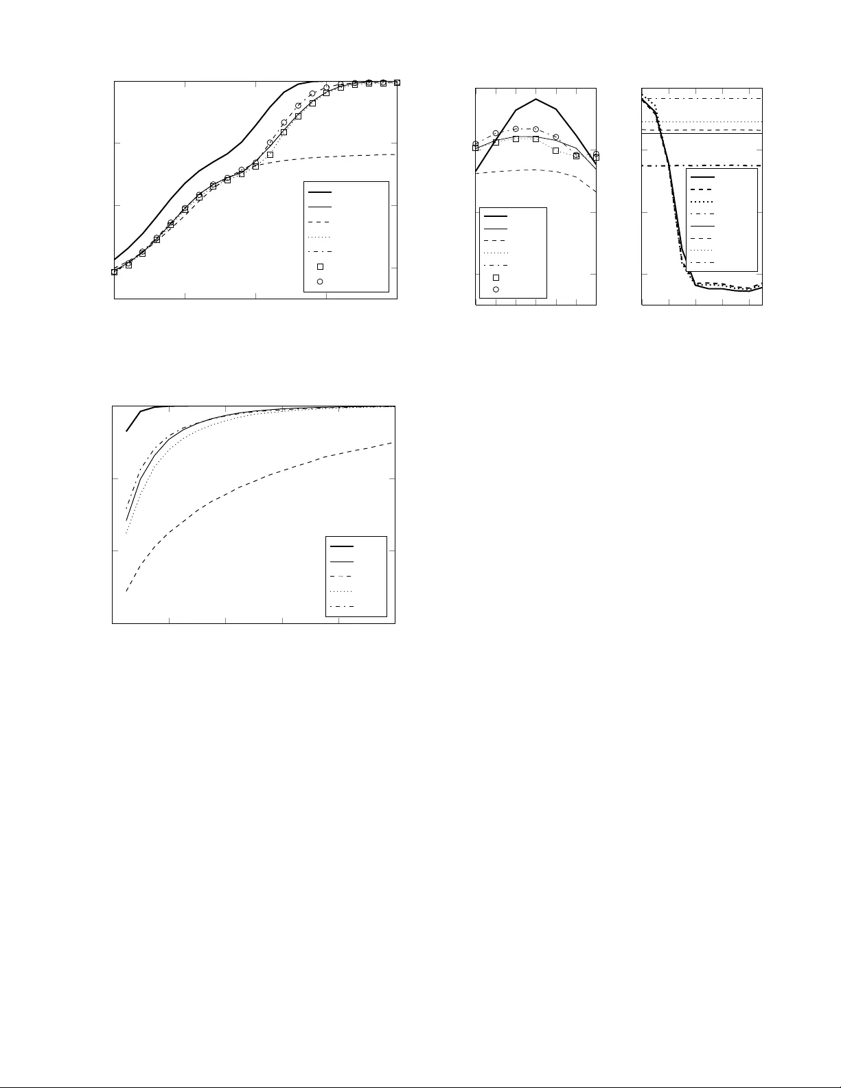
1 Computationally Ef ficient Modulation Le v el Classification Based on Probability Distrib ution Distance Functions Paulo Urriza, Eric Rebeiz, Przemysław Pawełczak, and Danijela ˇ Cabri ´ c Abstract —W e present a novel modulation level classifica- tion (MLC) method based on pr obability distrib ution distance functions. The proposed method uses modified Kuiper and Kolmogor ov-Smirno v distances to achieve low computational complexity and outperf orms the state of the art methods based on cumulants and goodness-of-fit tests. W e deriv e the theoretical performance of the pr oposed MLC method and verify it via simulations. The best classification accuracy , under A WGN with SNR mismatch and phase jitter , is achieved with the proposed MLC method using Kuiper distances. I . I N T RO D U C T I O N Modulation le vel classification (MLC) is a process which detects the transmitter’ s digital modulation le vel from a re- ceiv ed signal, using a priori knowledge of the modulation class and signal characteristics needed for do wncon version and sampling. Among many modulation classification methods [1], a cumulant (Cm) based classification [2] is one of the most widespread for its ability to identify both the modulation class and lev el. Howe ver , differentiating among cumulants of the same modulation class, but with different le vels, i.e. 16QAM vs. 64QAM, requires a large number of samples. A recently proposed method [3] based on a goodness-of-fit (GoF) test using K olmogorov-Smirnov (KS) statistic has been suggested as an alternativ e to the Cm-based level classification which require lower number of samples to achieve accurate MLC. In this letter , we propose a nov el MLC method based on distribution distance functions, namely Kuiper (K) [4] [5, Sec. 3.1] and KS distances, which is a significant simplification of methods based on GoF . W e show that using a classifier based only on K-distance achieves better classification than the KS-based GoF classifier . At the same time, our method requires only 2 M L additions in contrast to 2 M (log 2 M + 2 K ) additions for the KS-based GoF test, where K is the number of distinct modulation lev els, M is the sample size and L  M is the number of test points used by our method. I I . P R O P O S E D M L C M E T H O D A. System Model Follo wing [3], we assume a sequence of M discrete, complex, i.i.d. and sampled baseband symbols, s ( k ) , [ s ( k ) 1 · · · s ( k ) M ] , drawn from a modulation order M k ∈ {M 1 , . . . , M K } , transmitted over A WGN channel, perturbed by uniformly distributed phase jitter and attenuated by an unknown factor A > 0 . Therefore, the recei ved signal is given as r , [ r 1 · · · r M ] , where r n = Ae j Φ n s n + g n , { g n } M n =1 ∼ The authors are with the Department of Electrical Engineering, Univer - sity of California, Los Angeles, 56-125B Engineering IV Building, Los Angeles, CA 90095-1594, USA (email: { pmurriza, rebeiz, przemek, dani- jela } @ee.ucla.edu). C N  0 , σ 2  and { Φ n } M n =1 ∼ U ( − φ, + φ ) . The task of the modulation classifier is to find M k , from which s ( k ) was drawn, given r . Without loss of generality , we consider unit power constellations and define SNR as γ , A 2 /σ 2 . B. Classification based on Distribution Distance Function The proposed method modifies MLC technique based on GoF testing using the KS statistic [3]. Since the KS statistic, which computes the minimum distance between theoretical and empirical cumulativ e distribution function (ECDF), re- quires all CDF points, we postulate that similarly accurate classification can be obtained by ev aluating this distance using a smaller set of points in the CDF . Let z , [ z 1 · · · z N ] = f ( r ) where f ( · ) is the chosen feature map and N is the number extracted features. Possible feature maps include | r | (magnitude, N = M ) or the concatenation of <{ r } and ={ r } (quadrature, N = 2 M ). The theoretical CDF of z giv en M k and γ , F k 0 ( z ) , is assumed to be known a priori (methods of obtaining these distributions, both empirically and theoretically , are presented in [3, Sec. III-A]). The K CDFs, one for each modulation level, define a set of test points t (  ) ij = arg max z D (  ) ij ( z ) , (1) with the distribution distances gi ven by D (  ) ij ( z ) = ( − 1)   F i 0 ( z ) − F j 0 ( z )  , (2) for 1 ≤ i, j ≤ K , i 6 = j , and  ∈ { 0 , 1 } , corresponding to the maximum positi ve and negativ e deviations, respectiv ely . Note the symmetry in the test points such that t (0) j i = t (1) ij . Thus, there are L , 2  K 2  test points for a K order classification. The ECDF , given as F N ( t ) = 1 N N X n =1 I ( z n ≤ t ) , (3) is ev aluated at the test points to form F N , { F N ( t (  ) ij ) } , 1 ≤ i, j ≤ K , i 6 = j . Here, I ( · ) equals to one if the input is true, and zero otherwise. By ev aluating F N ( t ) only at the test points in (1), we get ˆ D (  ) ij = ( − 1)   F N  t (  ) ij  − F j 0  t (  ) ij  (4) which are then used to find an estimate of the maximum positiv e and negati ve de viations ˆ D (  ) j = max 1 ≤ i ≤ K,i 6 = j ˆ D (  ) ij , 1 ≤ j ≤ K, (5) of the ECDF to the true CDFs. The operation of finding the ECDF at the giv en testpoints (4) can be implemented using 2 a simple thresholding and counting operation and does not require samples to be sorted as in [3]. The metrics in (5) are used to find the final distribution distance metrics ˆ D j = max     ˆ D (0) j    ,    ˆ D (1) j     , ˆ V j =    ˆ D (0) j + ˆ D (1) j    , (6) which are the reduced comple xity versions of the KS distance (rcKS) and the K distance (rcK), respectiv ely 1 . Finally , we use the metrics in (6) as substitutes to the true distance-based classifiers with the following rule: choose M ˆ k such that ˆ k D = arg min 1 ≤ j ≤ K ˆ D j , ˆ k V = arg min 1 ≤ j ≤ K ˆ V j . (7) In the remainder of the letter , we define h ˆ D ( F N ) = ˆ k D and h ˆ V ( F N ) = ˆ k V , where ˆ k D , ˆ k V ∈ { 1 , . . . , K } . C. Analysis of Classification Accuracy Let t , [ t 1 · · · t L ] denote the set of test points, { t (  ) ij } , sorted in ascending order . For notational consistency , we also define the following points, t 0 , −∞ and t L +1 , + ∞ . Given that these points are distinct, they partition z into L + 1 regions. An individual sample, z n , can be in region l , such that t l − 1 < z n ≤ t l , with a giv en probability , determined by F k 0 ( z ) . Assuming z n are independent of each other, we can con- clude that gi ven z , the number of samples that fall into each of the L + 1 regions, n , [ n 1 · · · n L +1 ] , is jointly distributed according to a multinomial PMF gi ven as f ( n | N , p ) =    N ! p n 1 1 ··· p n L +1 L +1 n 1 ! ··· n L +1 ! , if L +1 P i =1 n i = N , 0 , otherwise , (8) where p , [ p 1 · · · p L +1 ] , and p l is the probability of an individual sample being in region l . Giv en that z is drawn from M k , p l = F k 0 ( t l ) − F k 0 ( t l − 1 ) , for 0 < l ≤ L + 1 . Now , with particular n , the ECDF at all the test points is F N ( n ) , [ F N ( t 1 ) · · · F N ( t L )] , F N ( t l ) = 1 N l X i =1 n i . (9) Therefore, we can analytically find the probability of classifi- cation to each of the K classes as Pr( ˆ k = κ |M k ) = X n ∈ N L +1 I ( h ˆ V ( F N ( n )) = κ ) f ( n | N , p ) , (10) for the rcK classifier . A similar expression can be applied to rcKS, replacing h ˆ V ( · ) with h ˆ D ( · ) in (10). D. Complexity Analysis Giv en that the theoretical CDFs change with SNR, we store distinct CDFs for W SNR values for each modulation lev el (impact of the selection of W on the accurac y is discussed further in Section III-B.) Further, we store K W theoretical CDFs of length ¯ N each. For the non-reduced complexity classifiers that require sorting samples, we use a sorting algorithm whose complexity is N log N . From T able I, we 1 Note, that other non-parametric distances used in hypothesis testing exist (see introduction in e.g. [4]), although for bre vity they are not addressed here. W e note, howe ver , that our approach is easily applied to any assumed distance metric. T ABLE I N U MB E R O F O P E R A T IO N S A N D M E M ORY U S AG E Method Multiply Add Memory Cm 6 M 6 M K rcKS/rcK 0 2 M L W L ( K + 1) KS/K 0 2 M (log 2 M + 2 K ) K W ¯ N rcKS/rcK (mag) 2 M M ( L + 1) W L ( K + 1) KS/K (mag) 2 M M (log M + 2 K + 1) K W ¯ N see that for K ≤ 3 rcK/rcKS tests use less addition operations than K/KS-based methods [3] and Cm-based classification [2]. For K > 3 , the rcK method is more computationally ef ficient when implemented in ASIC/FPGA, and is comparable to Cm in complexity when implemented on a CPU. In addition, the processing time would be shorter for an ASIC/FPGA imple- mentation, which is an important requirement for cognitive radio applications. Furthermore, their memory requirements are also smaller since ¯ N has to be large for a smooth CDF . It is worth mentioning that the authors in [3] used the theoretical CDF , b ut used ¯ N as the number of samples to generate the CDF in their complexity figures. The same observation fav oring the proposed rcK/rcKS methods holds for the magnitude-based (mag) classifiers [3, Sec III-A]. I I I . R E S U LT S As an example, we assume that the classification task is to distinguish between M-QAM, where M ∈ { 4 , 16 , 64 } . For comparison we also present classification result based on maximum likelihood estimation (ML). A. Detection P erformance versus SNR In the first set of experiments we e valuate the performance of the proposed classification method for dif ferent values of SNR. The results are presented in Fig. 1. W e assume fix ed sample size of M = 50 , in contrast to [3, Fig. 1] to e valuate classification accuracy for a smaller sample size. W e confirm that e ven for small sample size, as sho wn in [3, Fig. 1], Cm has unsatisfying classification accuracy at high SNR. In (10,17) dB region rcK clearly outperforms all detection techniques, while as SNR exceeds ≈ 17 dB all classification methods (except Cm) con ver ge to one. In low SNR region, (0,10) dB, KS, rcKS, rcK perform equally well, with Cm having comparable performance. The same observation holds for lar ger sample sizes, not shown here due to space constraints. Note that the analytical performance metric de veloped in Section II-C for rcK and rcKS matches perfectly with the simulations. For the remaining results, we set γ = 12 dB, unless otherwise stated. B. Detection P erformance versus Sample Size In the second set of experiments, we e valuate the perfor- mance of the proposed classification method as a function of sample size M . The result is presented in Fig. 2. As observed in Fig. 1, also here Cm has the worst classification accuracy , e.g. 5% belo w upper bound at M = 1000 . The rcK method performs best at small sample sizes, 50 ≤ M ≤ 300 . With M > 300 , the accuracy of rcK and KS is equal. Classification based on rcKS method consistently falls slightly below rcK and KS methods. In general, rcKS, rcK and KS con verge to one at the same rate. 3 . . . . . 0 . 5 . 10 . 15 . 20 . 0 . 4 . 0 . 6 . 0 . 8 . 1 . SNR γ (dB) . Probability of Correct Classification . . . . ML . . . KS . . . Cm . . . rcKS . . . rcK . . . rcKS (an.) . . . rcK (an.) Fig. 1. Effect of v arying SNR on the probability of classification with M =50; (an.) – analytical result using (10). . . . . . 0 . 200 . 400 . 600 . 800 . 1 , 000 . 0 . 7 . 0 . 8 . 0 . 9 . 1 . Sample Size N . Probability of Correct Classification . . . . ML . . . KS . . . Cm . . . rcKS . . . rcK Fig. 2. Effect of varying sample size on the probability of classification with γ = 12 dB. C. Detection P erformance vs SNR Mismatch and Phase Jitter In the third set of e xperiments we e valuate the performance of the proposed classification method as a function of SNR mismatch and phase jitter . The result is presented in Fig. 3. In case of SNR mismatch, Fig. 3(a), our results show the same trends as in [3, Fig. 4]; that is, all classification methods are relativ ely immune to SNR mismatch, i.e. the difference between actual and maximum SNR mismatch is less than 10% in the considered range of SNR values. This justifies the selection of the limited set of SNR values W for complexity ev aluation used in Section II-D. As expected, ML sho ws v ery high sensitivity to SNR mismatch. Note again the perfect match of analytical result presented in Section II-C with the simulations. In the case of phase jitter caused by imperfect downcon ver - sion, we present results in Fig. 3(b) for γ = 15 dB as in [2], in contrast to γ = 12 dB used earlier, for comparison purposes. . . . . . . γ − 2 . γ − 1 . γ . γ + 1 . γ + 2 . . 0 . 4 . 0 . 6 . 0 . 8 . 1 . SNR mismatch (dB) . Probability of Correct Classification . . . . ML . . . KS . . . Cm . . . rcKS . . . rcK . . . rcKS (an.) . . . rcK (an.) (a) . . . . . 0 . 20 . 40 . 60 . 80 . 0 . 4 . 0 . 6 . 0 . 8 . 1 . ϕ ( ◦ ) . . . . KS . . . rcKS . . . rcK . . . Cm . . . KS (mag) . . . rcKS (mag) . . . rcK (mag) . . . ML (mag) (b) Fig. 3. (a) Effect of SNR mismatch, nominal/true SNR=12dB; (b) effect of phase jitter , nominal SNR=15dB.; (an.) – analytical result using (10), (mag) – magnitude. W e observe that our method using the magnitude feature, rcK/rcKS (mag), as well as the Cm method, are in variant to phase jitter . rcK and rcKS perform almost equally well, while Cm is worse than the other three methods by ≈ 10%. As expected, the ML performs better than all other methods. Quadrature-based classifiers, as expected, are highly sensiti ve to phase jitter . Note that in the small phase jitter , φ < 10 ◦ , quadrature-based classifiers perform better than others, since the sample size is twice as large as in the former case. I V . C O N C L U S I O N In this letter we presented a nov el, computationally efficient method for modulation level classification based on distribu- tion distance functions. Specifically , we proposed to use a metric based on K olmogorov-Smirno v and Kuiper distances which e xploits the distance properties between CDFs corre- sponding to different modulation lev els. The proposed method results in faster MLC than the cumulant-based method, by reducing the number of samples needed. It also results in lower computational complexity than the KS-GoF method, by eliminating the need for a sorting operation and using only a limited set of test points, instead of the entire CDF . R E F E R E N C E S [1] O. A. Dobre, A. Abdi, Y . Bar-Ness, and W . Su, “Surve y of automatic mod- ulation classification techniques: Classical approaches and new trends, ” IET Communications , vol. 1, no. 2, pp. 137–156, Apr. 2007. [2] A. Swami and B. M. Sadler, “Hierarchical digital modulation classifica- tion using cumulants, ” IEEE T rans. Commun. , v ol. 48, no. 3, pp. 416–429, Mar . 2000. [3] F . W ang and X. W ang, “Fast and robust modulation classification via Kolmogorov-Smirnov test, ” IEEE T rans. W ir eless Commun. , vol. 58, no. 8, pp. 2324–2332, Aug. 2010. [4] G. A. P . Cirrone, S. Donadio, S. Guatelli, A. Mantero, B. Masciliano, S. Parlati, M. G. Pia, A. Pfeiffer, A. Ribon, and P . V iarengo, “ A goodness of fit statistical toolkit, ” IEEE T rans. Nucl. Sci. , v ol. 51, no. 5, pp. 2056– 2063, Oct. 2004. [5] M. A. Stephens, “EDF statistics for goodness of fit and some compar- isons, ” Journal of the American Statistical Association , vol. 69, no. 347, pp. 730–737, Sep. 1974.