Understanding 3-manifolds in the context of permutations

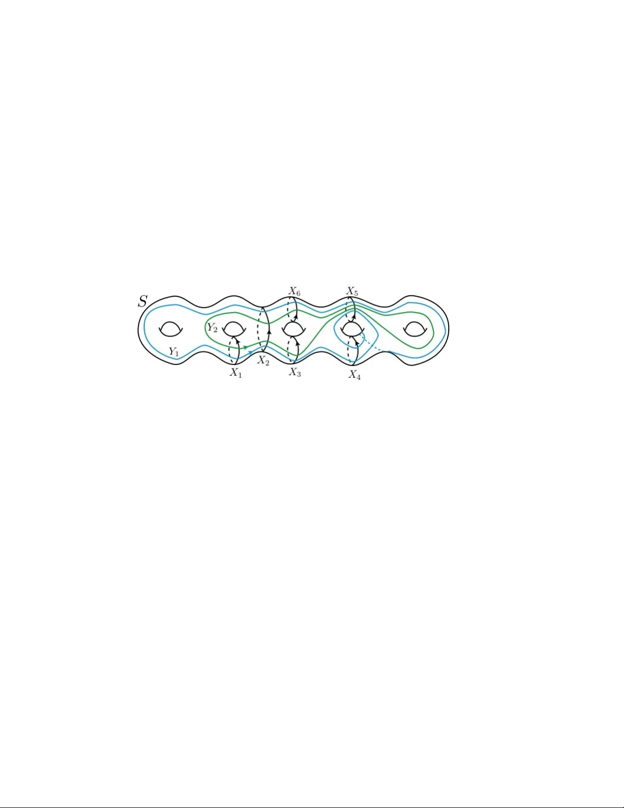
UNDERST ANDING 3-MANIF OLDS IN THE CONTEXT OF PERMUT A TIONS KAR OLINE NULL Abstract. W e demonstrate ho w a 3-manifold, a Heegaard diagram, and a group presen- tation can eac h be in terpreted as a pair of signed p ermutations in the symmetric group S d . W e demonstrate the p o wer of p erm utation data in programming and discuss an algorithm w e hav e developed that takes the permutation data as input and determines whether the data represen ts a closed 3-manifold. W e therefore ha ve an in v ariant of groups, that is giv en an y group presentation, we can determine if that presen tation presen ts a closed 3-manifold. 1. Introduction Since there inception, three-manifolds ha v e b een inv estigated through Heegaard dia- grams, splittings, and groups. T ranslating a 3-manifold to a diagram pro vides a nice 2-dimensional means of dealing with a difficult 3-dimensional ob ject. W orking with a 3- manifold in terms of groups is also a w a y of translating the problem from top ology into algebra, allo wing another field of techniques to b e applied to this study . W e in troduce a technique to translate b et w een group presen tations, diagrams (and hence Heegaard splittings) and pairs of signed p erm utations. This was first done b y Montesino [Mon83] and then b y Hemp el [Hem04] for p ositiv e Heegaard diagrams, but little has been done with this approac h since then, no doubt b ecause of the tedious calculations that w ere required. With the now nearly universal a v ailabilit y of fast computers, p erm utations should b e revisited as they pro vide a quic k computational approac h to dealing with 3-manifolds. P erm utation data is amenable to algorithmic sorting and chec king tec hniques, th us with the newfound a v ailability of fast computing p o wer, we revisit p erm utation data as a wa y of enco ding Heegaard diagrams, and hence 3-manifolds. It has b een shown (see [P er09]) that the problem of deciding whether a group presentation P presents a closed 3-manifold is recursiv ely en umerable. In this pap er, w e shall determine the decidabilit y of whether a fixed P presents a 3-manifold group. Ev ery presen tation is determined by a family of Heegaard diagrams. W e w an t to decide whether the presentation do es indeed present the fundamen tal group of a 3-manifold de- termined by one of these Heegaard diagrams. W e explicitly state the characteristics of this Date : May 21, 2019. 2010 Mathematics Subje ct Classific ation. 57N65, 57M05, 57M27, 57M60, 22F30, 22F50, 22F05, 20B10, 22C05. Key wor ds and phr ases. 3-manifolds, Heegaard Diagrams, p erm utations. This paper is from the author’s do ctoral dissertation. 1 2 KAROLINE NULL family of diagrams asso ciated to a trivially reduced presentation. These are the classes to examine, finite and infinite. The infinite class of diagrams is treated in [P er09]. The finite class, made up of every p ossible curv e re-ordering on the diagram determined by P , will b e treated here. Any diagram determines a finite n umber (or a family ) of signed p erm utation pairs, which are in one-to-one corresp ondence with this finite class. Beginning with only a pair of signed p erm utations, we determine whether the asso ciated 3-manifold is closed (Lemma 7.4). W e hav e a metho d for pro ducing a set of signed p erm utation data to enco de a presen- tation ( § 5), and dev elop ed an algorithm that pro duces this finite family and determines if an y diagram from the finite family results in S − X b eing planar ( § 6). The algorithm is a v ailable up on request. 2. Preliminaries Definition 2.1. Let B n denote the unit ball { x ∈ R n : || x || ≤ 1 } , and S n − 1 denote the unit sphere { x ∈ R n : || x || = 1 } . W e call a space homeomorphic to B n an n -c el l , and a space homeomorphic to S n − 1 an ( n − 1) -spher e . A (topological) n -manifold is a separable metric space, eac h of whose points has an op en neigh b orhoo d homeomorphic to either R n or R n + = { x ∈ R n : x n ≥ 0 } . The b oundary of an n -manifold M , denoted ∂ M , is the set of p oin ts of M having neigh b orho ods homeomorphic to R n + . By inv ariance of domain, ∂ M is either empt y or an n − 1 dimensional manifold and ∂ ∂ M = ∅ [Bro12]. A manifold M is close d if M is compact with ∂ M = ∅ and the manifold is op en if M has no compact component and ∂ M 6 = ∅ . A c ompr ession b o dy V is obtained from a connected surface S b y attaching 2-handles to S × { 0 } and capping off an y 2-sphere b oundary comp onen ts with 3-handles. W e define ∂ + V := S × { 1 } and ∂ − V = ∂ V − ∂ + V , the latter of which is also the result of surgery on S × { 0 } . A hand leb o dy is a compression b ody in which ∂ V is empty . Throughout this work, we assume all manifolds are oriented. Of in terest are 3-manifolds, because ev ery compact, orien ted 3-manifold has a splitting (see [Hem76] for a pro of ). Definition 2.2. A ( He e gaar d ) splitting is a representation of a connected 3-manifold M b y the union of tw o compression b odies V X and V Y , with a homeomorphism taking ∂ + V X to ∂ + V Y . The resulting 3-manifold can b e written M = V X ∪ S V Y , where S is the surface ∂ + V X = ∂ + V Y in M . W e call S the splitting surfac e and g ( S ) the genus of the splitting. As the Lens Spaces (gen us one) are effectively classified [PY03], we will only b e considering splittings of gen us ≥ 2 . Before w e formally define diagrams, we might do w ell to p oin t out that one w a y of viewing diagrams is as a to ol for splittings. Supp ose we ha v e a splitting of a 3-manifold 3-MANIFOLDS AS PERMUT A TIONS 3 M = V X ∪ S V Y . A diagram sho ws the attaching curv es for the 2-handles of V X and V Y . Ev ery compact, oriented, connected 3-manifold has a splitting, and for eac h splitting many differen t curve se ts could be c hosen to determine the compression b o dies. Th us, every 3-manifold can b e studied through tw o-dimensional diagrams. Ho w ever, we do not need to b egin with a splitting and mov e to the diagram. It is imp ortan t to consider diagrams abstractly , since throughout this w ork w e will begin with diagrams and determine prop erties of the asso ciated 3-manifold. Definition 2.3. A diagr am is an ordered triple ( S ; X , Y ) where S is a closed, oriented, connected surface and X := { X 1 , . . . , X m } and Y := { Y 1 , . . . , Y n } are compact, orien ted 1-manifolds in S in relativ e general p osition and for which no comp onen t of S − ( X ∪ Y ) is a bigon — a disc whose b oundary is the union of an arc in X and an arc in Y . Figure 1. An example of a diagram D = ( S ; X , Y ) with g ( S ) = 5 , m = 6 , and n = 2. This definition allo ws X (or Y ) to hav e sup erfluous curves , a subset of comp onen ts of X (or Y ) whic h could b ound a planar surface in S. W e allow this b ecause there is a corresp ondence b et w een diagrams and presen tations, under which the diagram for a 3-manifold asso ciated to the p erm utations may hav e sup erfluous curves. Tw o diagrams ( S ; X, Y ) and ( S ∗ ; X ∗ , Y ∗ ) are equiv alent provided g ( S ) = g ( S ∗ ) and there is a homeomorphism b et w een surfaces, taking X to X ∗ and Y to Y ∗ . An ar c is a comp onen t of Y − X on the surface of S. Giv en a diagram, the manifold M can b e reco v ered from the diagram as follows. F or eac h i = 1 , . . . , m attach a cop y of B 2 × I to S × [0 , 1] by identifying ∂ B 2 × I with a neigh b orhoo d of X i in S × { 0 } ⊂ S × [0 , 1] . F or each i = 1 , . . . , n attac h a copy of B 2 × I to S × [0 , 1] by identifying ∂ B 2 × I with a neighborho od of Y i in S × { 1 } ⊂ S × [0 , 1] . The resulting manifold, M 1 , has a 2-sphere boundary comp onen t for eac h planar region in S − X and S − Y . Obtain M by attaching a cop y of B 3 to each 2-sphere b oundary comp onen t of M 1 . W e will use this understanding of a diagram throughout this pap er, viewing a diagram as giving the splitting surface sitting in a 3-manifold, with X and Y b ounding discs on either side of S. A diagram also determines a presentation. 4 KAROLINE NULL Definition 2.4. Given a diagram D , the pr esentation determine d by D , denoted P ( D ) , is a finite group presen tation with one generator x i for eac h comp onen t X i ∈ X , and one relator for each comp onen t of Y i ∈ Y , defined b y recording the intersection with each X i , and p erforming any trivial reductions. That is, each relator is obtained as r i := x  1 i 1 x  2 i 2 . . . x  k ik , where the curve Y i crosses X i 1 , X i 2 , . . . , X ik in order with crossing num bers  i (see Figure 2). Figure 2. A p ositiv e crossing with  = 1 (left) and a negative crossing with  = − 1 (right) When relating this to π 1 ( M ) w e regard x i as a curve in S whic h crosses X i with a p ositiv e crossing num b er and which crosses no other X j . Instances of x i x − 1 i (or x − 1 i x i ) that app ear in the presen tation determined b y a diagram will often not b e replaced with 1 in a relator, unless otherwise sp ecified. Example 2.5. Consider the diagram D = ( S ; X , Y ) in Figure 1. As X = { X 1 , X 2 , X 3 , X 4 , X 5 , X 6 } , the presentation P ( D ) has six generators { x 1 , x 2 , x 3 , x 4 , x 5 , x 6 } . As Y = { Y 1 , Y 2 } , P ( D ) has tw o relators. W e record eac h by flowing along the curve and recording each generator encountered with a sup erscript of 1 if the crossing was p ositiv e, and − 1 if the crossing was negativ e (see Figure 2). Thus P ( D ) = h x 1 , x 2 , x 3 , x 4 , x 5 , x 6 : x − 1 1 x − 1 2 x − 1 3 x − 1 4 x 5 x − 1 4 x 5 x 6 x 2 , x 1 x − 1 2 x − 1 3 x − 1 5 x 5 x 6 x 2 i . T o force the construction of P ( D ) from D to b e well-defined, we set the conv en tion that the diagram ( S ; X , Y ) is an ordered triple, where X will alwa ys corresp ond to the generating set and Y will alwa ys corresp ond to the set of relators. The presentation determined b y a diagram is unique up to in version and cyclic reordering. It is well known that the group presen ted by the presen tation, denoted | P ( D ) | , is isomorphic to the fundamen tal group of the 3-manifold M determined by the presentation pro vided M is closed and X is a complete meridian set (see [Hem76] for a pro of ). 3. How a Heegaard diagram determines a set of oriented permut a tions Let ( S ; X , Y ) b e a diagram for a 3-manifold. The simple, closed, oriented curv es of X intersect with the simple, closed, oriented curves of Y in d p oin ts. By num bering the in tersection p oin ts 1 through d, we can enco de each X i of X and each Y j of Y by listing the n um b ered intersection p oin ts in the order in whic h they are encoun tered when flo wing along the orien tated curv e. F or eac h X i w e denote the ordered cycle of in tersection num bers 3-MANIFOLDS AS PERMUT A TIONS 5 as α i and for each Y j w e denote the ordered cycle as β j , making it p ossible to interpret α = α 1 α 2 . . . α m and β = β 1 β 2 . . . β n as elemen ts of S d , the symmetric group on d elemen ts. W e let c ( α ) denote the num b er of cycles in a p erm utation, so X and Y will hav e c ( α ) and c ( β ) comp onen ts resp ectiv ely (i.e. one simple closed curve on the surface corresp onds to one cycle in the resp ective p erm utation). W e let | α i | denote the length of the cycle α i . Since the curves in ( X ∪ Y ) are oriented, at eac h of the d p oin ts w e associate an in tersection n um b er ± 1 (see Figure 2) via the in tersection function . Definition 3.1. The interse ction function  : { 1 , 2 , . . . , d } → { 1 , − 1 } indicates X and Y hav e a p ositiv ely-orien ted crossing at i if  ( i ) = 1 , and indicates a negativ ely-orien ted crossing if  ( i ) = − 1 . W e call  ( i ) the interse ction numb er at i. F or exp ediency ,  is often written as a d -tuple of 1’s and − 1’s. W e call the triple ( α, β ,  ) a p ermutation data set for ( S ; X, Y ) . Notice that the p er- m utation data set asso ciated to a splitting is unique up to ren umbering, corresponding to b eing unique up to conjugation of α and β in S d . Let X i ha v e k i in tersection p oin ts for 1 ≤ i ≤ m, suc h that P k i = d. Our conv ention is to lab el the intersection points of X 1 consecutiv ely with 1 , 2 , . . . , k 1 ; to lab el the intersection p oin ts of X 2 consecutiv ely with ( k 1 + 1) , ( k 1 + 2) , . . . , ( k 1 + k 2 ); and so on, lab eling the in tersection p oin ts of X m consecutiv ely with K + 1 , K + 2 , . . . , d where K := k 1 + k 2 + . . . + k m − 1 . Example 3.2. Consider the diagram ( S ; X , Y ) sho wn in Figure 3. Lab el the in tersection p oin ts consecutiv ely , b eginning on X 1 . Then w e hav e α = α 1 α 2 = (1 , 2)(3 , 4 , 5 , 6) , β = β 1 β 2 = (1 , 6 , 4)(2 , 3 , 5) ,  = (1 , 1 , − 1 , − 1 , − 1 , − 1) . Figure 3. A diagram with intersection points lab eled 6 KAROLINE NULL 4. How a permut a tion da t a set determines a present a tion W e demonstrate how to construct P directly from ( α, β ,  ) without needing to create the diagram as an in termediate step. When necessary , w e use the notation P α,β , to mean the presen tation determined from the p erm utation data set ( α, β ,  ) . When giv en a diagram, conv en tion requires the X -curves to correspond to the generators and the Y -curves to corresp ond to the relators. Similarly , w e consider the cycles of α to b e the generators and the cycles of β to enco de the relators. Let α, β b e in S d , with c ( α ) = m, c ( β ) = n. Define the map a : { 1 , 2 , . . . , d } → { 1 , 2 , . . . , m } suc h that j ∈ α a ( j ) . The group presentation P α,β , is written P = h α 1 , α 2 , . . . , α m : r 1 , r 2 , . . . , r n i . Eac h β i := ( i 1 , i 2 , . . . , i k ) of β determines the relator r i := α  ( i 1 ) a ( i 1 ) α  ( i 2 ) a ( i 2 ) . . . α  ( i k ) a ( i k ) . Example 4.1. W e demonstrate how to determine P α,β , from ( α, β ,  ) . Let α = (1 , 2 , 3 , 4)(5 , 6 , 7)(8 , 9 , 10 , 11) , β = (1 , 6)(2 , 4 , 11)(8 , 5 , 10)(9 , 3 , 7) ,  = (1 , 1 , − 1 , − 1 , − 1 , 1 , − 1 , − 1 , 1 , 1 , 1) . As c ( α ) = 3 , and c ( β ) = 4 , P α,β , will hav e 3 generators and 4 relators: P α,β , = h x 1 , x 2 , x 3 : x 1 x 2 , x 1 x − 1 1 x 3 , x − 1 3 x − 1 2 x 3 , x 3 x − 1 1 x − 1 2 i . There is no am biguit y when we b egin with a p erm utation data set, since P α,β , is required to use precisely ( α , β ,  ) , so if α, β ∈ S d , then deg A ( P α,β , ) = d and no trivial reductions are p erformed. That is, P α,β , need not b e reduced as written. Ho w ever, when we begin with a presen tation as in § 5, P is alwa ys assumed to b e triv- ially reduced unless otherwise stated. Th us, given ( α, β ,  ) , P α,β , can only differ up to cyclic p erm utation of the relators or a re-ordering of the generators and relators in the presen tation, and w e consider all such presen tations to b e equiv alent. 5. A present a tion determines a class of permut a tion da t a sets The map sending a group presentation to a p erm utation data set is not well-defined, and with regard to the prop erties that we are interested in, all possible ( α, β ,  )’s determining P are not ev en “equiv alen t,” since some will allow us to construct a diagram for a closed 3-manifold and some will not. The fixed, reduced presen tation P does determine a finite n um b er of permutation data sets, each of which could determine a differen t curve set and diagram and therefore a differen t 3-manifold. W e consider all ( α, β ,  ) of degree d that determine a fixed P to b e in a class of p er- m utation data sets, which w e denote P d ( P ) , read as “the class of p erm utation data sets of degree d for presen tation P .” Not all ( α, β ,  ) ∈ P d ( P ) result in equiv alen t 3-manifolds, 3-MANIFOLDS AS PERMUT A TIONS 7 therefore when using signed permutation data to answ er whether P has a sp ecific property , w e only need to kno w that a single ( α, β ,  ) in the class P d ( P ) has the desired properties. Let P = h x 1 , x 2 , . . . , x m : r 1 , r 2 , . . . , r n i b e giv en. Let k i denote the num ber of times that x i (or x − 1 i ) app ears in the set of relators, and put P k i = d. Let α 1 = (1 , 2 , . . . , k 1 ) , α 2 = ( k 1 + 1 , k 1 + 2 , . . . , k 1 + k 2 ) , . . . α m = ( K + 1 , K + 2 , . . . , d ) , where again K := k 1 + k 2 + . . . + k m − 1 . A relator r j is recorded in the cycle β j b y assigning each o ccurrence of a generator x i a unique entry from α i . One conv en tion would b e to record the low est n um b ered elemen t of α i that has not yet b een used for eac h x i w e encoun ter, but other conv en tions will provide the other ( α, β ,  )’s whic h determine P . Finally , as w e assign a num b er i for each generator x i in r j , record the sign of x i in  ( i ) . Example 5.1. W e no w demonstrate how to get one ( α, β ,  ) that determines P . Consider the presentation for the Heisen b erg group H 3 := h x, y , z : [ x, y ] z − 1 , [ x, z ] , [ y , z ] i . Let α 1 corresp ond to x, α 2 corresp ond to y , and α 3 corresp ond to z . The length of eac h cycle in α represents the num ber of times the corresp onding generator is used in a relator so we ha v e α = α 1 α 2 α 3 = (1 , 2 , 3 , 4)(5 , 6 , 7 , 8)(9 , 10 , 11 , 12 , 13) . Record the relators as cycles of β , alw a ys using the lo w est unused num be r from the appro- priate α i , β = β 1 β 2 β 3 = (1 , 5 , 2 , 6 , 9)(3 , 10 , 4 , 11)(5 , 12 , 6 , 13) . Finally , record the sign of each generator x i in to  ( i ) ,  = (1 , − 1 , 1 , − 1 , 1 , − 1 , 1 , − 1 , − 1 , 1 , − 1 , 1 , − 1) . W e force the pro cess of going from P to ( α, β ,  ) to b e well-defined b y letting the con- v en tion b e to record the elemen ts of β j b y using up the elements from α i c onse cutively . The ill definedness comes from the ambiguit y in choosing some unused element of α i for eac h x i in r j while recording β j . The class of p erm utation data sets P d ( P ) is the collection of all suc h p ossibilities for β j . W e next demonstrate how to go from a set of p erm utation data to a splitting. When w e consider § 5 and § 6 together, w e hav e a wa y to b egin with an arbitrary group presentation, translate P in to a pair of signed p erm utations, and determine prop erties ab out the 3- manifold M α,β , . 8 KAROLINE NULL 6. How a permut a tion da t a set determines a diagram This section is exciting b ecause we b egin with the minimum data required to build a 3-manifold. Given tw o p erm utations α, β ∈ S d , and a function  : { 1 , 2 , . . . , d } → { 1 , − 1 } , w e describ e how to build ( S ; X , Y ) by constructing the splitting surface S and letting α and β define curve sets X and Y . Th us the p erm utation data set ( α, β ,  ) is a combinatorial represen tation of a diagram D , whic h uniquely determines M ( D ) . W e first construct the splitting surface by viewing each p erm utation as a set of simple, closed, oriented curves crossed with in terv als, intersecting the t wo p erm utations appropriately , and then capping off the b oundary comp onen ts of this frame. So long as α and β generate a transitive subgroup in S d , the ribb on diagram (defined next) will b e connected and hence the manifold will b e connected. If α and β do not generate a transitiv e subgroup, then partition the cycles of α and β suc h that eac h partition is a subset of cycles that do create a transitive subgroup of S d , ren um b ering as appropriate and creating new intersection functions that retain the crossing information. Each new set of p erm utation data will result in a connected manifold, and the original p erm utation data set corresp onds to a connected sum of these manifolds. F or the rest of this pap er, we will assume the p erm utations generate a transitiv e subgroup of S d . 6.1. Building the splitting surface from ( α, β ,  ) . Let ( α, β ,  ) b e a p erm utation data set with c ( α ) = m, c ( β ) = n, and α, β ∈ S d . Giv en ( α , β ,  ) , we construct a ribb on diagr am , ˜ R α,β , (or just ˜ R ), as follo ws: (1) F or each cycle α i = ( i 1 , i 2 , . . . , i k ) of α, take an orien ted simple closed curve X i and lab el p oin ts i 1 , i 2 , . . . , i k in order around X i . Do the same for eac h cycle β j of β to get Y j . (2) Define a ribb on, ˜ r ( X i ) := X i × [0 , 1] , or ˜ r ( Y j ) := Y j × [0 , 1] . Notice there is one ribb on for each cycle of a p erm utation. (3) As eac h ribbon is no w a surface, at each p oin t i ∈ { 1 , . . . , d } , the oriented interv al i × [0 , 1] is a normal v ector. The ordered pair ( X i , [0 , 1]) puts an orientation on the ribb on surface. (4) F or eac h i choose an orien ted interv al neigh borho o d U i of i, U i in X and an orien ted in terv al neighborho od V i of i, V i in Y . Identify ( U i × [0 , 1]) with ( V i × [0 , 1]) by an orien tation preserving pro duct homeomorphism • which tak es U i to ( i × [0 , 1]) , and ( i × [0 , 1]) to + V i if  ( i ) = +1 , and • which tak es U i to ( i × [0 , 1]) , and ( i × [0 , 1]) to − V i if  ( i ) = − 1 . (5) Let ˜ R, the ribb on diagram, b e this iden tified space. 6.2. Calculating the genus of the splitting surface. The b oundary comp onen ts of ˜ R are p olygons, with edges from ribb ons ˜ r ( X i ) and ˜ r ( Y j ) . W e obtain S from ˜ R b y capping off the b b oundary comp onen ts of ˜ R with 2-cells, denoted e 2 , so S = ˜ R b [ k =1 e 2 k . 3-MANIFOLDS AS PERMUT A TIONS 9 Figure 4. Identifying the neigh b orhoo ds U i × [0 , 1] and V i × [0 , 1] , hence  ( i ) = +1 The gen us of S is determined from the Euler c haracteristic of ˜ R ∪ e 2 k . First note that χ ( ˜ R ) = − d, as ˜ R collapses to a graph with d vertices and 2 d edges. By capping off a b oundary com ponent (i.e. adding a 2-cell), w e add one to the Euler c haracteristic. Therefore, by counting the n um b er of b oundary comp onen ts we can calculate the Euler c haracteristic of S = ˜ R ∪ e 2 k and the gen us of S. F or 1 ≤ i ≤ d, eac h neigh b orhoo d U i in ˜ R o ccurs at the intersection of some ribb ons ˜ r ( X i ) and ˜ r ( Y j ) . Such an in tersection creates four quadrants and each quadrant will app ear exactly once in S as the corner of a b oundary region. Quadrants are num bered 1 through 4 as sho wn in Figure 5. Figure 5. Quadran t lab els for a p ositiv e crossing (left) and a negative crossing (right) Beginning at a p oin t i and quadrant Q, w e flow along the b oundary of ˜ R in the coun- terclo c kwise direction, recording the ( i, Q ) corners in that comp onen t of ∂ ˜ R. W e get a p erm utation φ of the elemen ts { ( i, Q ) : i = 1 , . . . , d, Q = 1 , 2 , 3 , 4 } , where each b oundary comp onen t of ˜ R corresp onds to an orbit of this p erm utation. T o coun t the num ber of b oundary comp onen ts, w e consider the 4 d ordered pairs ( i, Q ) , and partition them into orbits by noticing the precise rules dictating how one corner flo ws in the p ositiv e direction to the next. The algorithm for partitioning the ordered pairs is next and the 16 p ossible outcomes are summarized in T able 1. Algorithm. T o c ompute the elements in an orbit 10 KAROLINE NULL (1) Beginning in a quadrant, ( i, Q ) , apply the p erm utation to determine the next cor- ner, ( i 0 , Q 0 ) . (2) The map φ is a separate map on each co ordinate: φ ( i, Q ) = ( φ 1 ( i, Q,  ( i )) , φ 2 ( Q,  ( i 0 ))) , with φ 1 ( i, Q,  ( i )) ∈ { 1 , 2 , . . . d } , and φ 2 ( Q,  ( i 0 )) ∈ { 1 , 2 , 3 , 4 } . (3) The in tersection n um b er and quadran t determine whic h edge we flo w along to get to the next corner. The edge w e flo w along from i determines the p erm utation w e apply to i, so as to determine the next corner, i 0 . The edge X  corresp onds to ev aluating α  ( i ) , and the edge Y  corresp onds to ev aluating β  ( i ) . (4) The new quadran t Q 0 is determined by the quadrant we started from, Q, and the in tersection num ber of the new corner,  ( i 0 ) . (5) When finished, we will partitioned the 4 d corners into b orbits, with eac h orbit corresp onding to a boundary comp onen t of ˜ R. Capping eac h b oundary comp onen t of ˜ R gives us the closed, oriented splitting surface S. W e hav e a diagram ( S ; X, Y ) , with χ ( S ) = χ ( ˜ R ) + b, for the b 2-cells attac hed to ∂ ˜ R. Th us we ha ve the following lemma. Lemma 6.1. L et ( α, β ,  ) b e given. Then ( α, β ,  ) determines a diagr am ( S ; X , Y ) for a 3-manifold, with S the splitting surfac e of genus g ( S ) = 1 2 ( b − d + 2) . 7. Determining when M α,β , is closed and connected Beginning with just a pair of signed p erm utations, w e ha ve constructed the diagram D = ( S ; X , Y ) for a splitting of M α,β , (or just M .) W e use planar to indicate that a surface embeds in R 2 . If S − X can b e embedded in R 2 , then it will b e a punctured sphere, whic h can b e dra wn in the plane (as well as an y em b edded curves in S − X ), and hence “planar.” The manifold M will b e closed if and only if eac h comp onen t of S − X and of S − Y is planar. In this section, we dev elop a means of determining whether S − X and S − Y are planar, so as to conclude that M α,β , is closed. Consider compressing along the disc determined b y a simple closed curv e, X i on S. Compression along X i either separates S or reduces the genus of S b y one. If S − X is one comp onen t, then no X i separates S and each simple closed curve in X that w e compress along will reduce g ( S ) by one. Thus, if S − X is connected and X contains g ( S ) distinct curv es, then S − X is planar. When S − X (or S − Y ) has more than one comp onen t, M will still b e closed provided eac h comp onen t is planar. Eac h non-planar comp onen t will determine a b oundary comp onen t of M . In the last section, given ( α, β ,  ) we partitioned the 4 d corners in to b oundary comp o- nen ts of the ribb on diagram, which corresp onded to the b oundary of the complemen tary comp onen ts of S − ( X ∪ Y ) . W e no w place t w o b oundary comp onen ts of S − ( X ∪ Y ) into an orbit class if they are in the same comp onen t of S − X . W e then calculate the Euler c haracteristic of each orbit class to determine whether the comp onen t is planar. At the end, we will replicate this pro cess to determine whether S − Y has planar comp onen ts, but for now w e are considering only the comp onen ts of S − X . 3-MANIFOLDS AS PERMUT A TIONS 11  ( i ) Q φ 1 ( i, Q,  ( i ))  ( i 0 ) φ 2 ( Q,  ( i 0 )) Illustration +1 1 α ( i ) +1 2 +1 1 α ( i ) -1 3 +1 2 β ( i ) +1 3 +1 2 β ( i ) -1 4 +1 3 α − 1 ( i ) +1 4 +1 3 α − 1 ( i ) -1 1 +1 4 β − 1 ( i ) +1 1 +1 4 β − 1 ( i ) -1 2 -1 1 β ( i ) +1 3 -1 1 β ( i ) -1 4 -1 2 α − 1 ( i ) +1 4 -1 2 α − 1 ( i ) -1 1 -1 3 β − 1 ( i ) +1 1 -1 3 β − 1 ( i ) -1 2 -1 4 α ( i ) +1 2 -1 4 α ( i ) -1 3 T able 1. Rules for tracing around a comp onen t of S − ( X ∪ Y ) 12 KAROLINE NULL T o create the classes of orbits, each corresp onding to a comp onen t of S − X, we add the Y -curv es into S − ( X ∪ Y ) one at a time. As we replace a Y -curv e, we notice that quadran ts on opp osite sides of the Y -curve will b e identified. Hence tw o comp onen ts of S − ( X ∪ Y ) will b e iden tified if they were adjacent across a Y -curv e. W e iden tify quadran ts algebraically by noting that remo ving a Y -curv e corresp onds to iden tifying quadran ts 1 and 2 , and identifying quadran ts 3 and 4 , regardless of whether a crossing is p ositiv e or negativ e. That is, place the orbits con taining the p oin ts ( i, 1) and ( i, 2) in the same orbit class, and the orbits con taining ( i, 3) and ( i, 4) in the same orbit class. Figure 6. Identifying corners ( i, 1) ≡ ( i, 2) and ( i, 3) ≡ ( i, 4) when Y - curv es are replaced When all 2 d identifications hav e b een made, the num ber of orbit classes of b oundary comp onen ts will b e the n um b er of comp onen ts of S − X . When coun ting the num ber of comp onen ts of S − X , it is useful to tag eac h X -curv e, meaning for eac h X  i , choose a corner ( i, Q ) to track X  i . Example 7.1. If α 1 = (1 , 2 , 3 , 4) and  (1) = 1 , then (1 , 1) can tag X + 1 and (1 , 3) can tag X − 1 . If  (1) = − 1 , then (1 , 3) could tag X + 1 and (1 , 1) could tag X − 1 . Within eac h comp onen t, we will need to count the num ber of tags, t, b ecause each tag corresp onds to one side of an X -curv e, and we cap each side of eac h X -curve with a 2-cell whic h affects the Euler c haracteristic of that comp onen t. The complimen tary comp onen ts of S − ( X ∪ Y ) are p olygons, whic h w e denote p i . Let [ κ x ] = { p 1 , p 2 , . . . p n } denote an orbit class of p olygonal comp onen ts. Then [ κ x ] corresp onds to one comp onen t of S − X , call it κ x , once w e make the appropriate iden tifications b et w een the p i ∈ [ κ x ] . T o calculate the Euler characteristic of S − X , we m ust calculate the Euler c haracteristic of eac h κ x . The comp onen t κ x is made b y identifying Y -edges b et ween p olygons in [ κ x ] , calculating the Euler c haracteristic after eac h identification and finally capping b oundary comp onen ts with discs. This is equiv alen t to • totaling the vertices V , edges E , and faces F for all of the disjoint polygons p i ; • subtracting t w o from V and one from E for each Y identification made; • adding one to F for each tag in κ x . Th us we ha ve the following lemma and corollary . 3-MANIFOLDS AS PERMUT A TIONS 13 Lemma 7.2. L et [ κ x ] = { p 1 , p 2 , . . . , p n } b e an orbit class of p olygonal b oundary c omp onents of S − ( X ∪ Y ) . L et m b e the numb er of matche d Y -e dges within the orbit class, and t b e the numb er of tags in κ x . Then the Euler char acteristic of this c omp onent, is χ ( κ x ) = n − m + t. Corollary 7.3. The c omp onent κ x has genus g ( κ x ) = 1 − 1 2 ( n − m + t ) . T o determine the total genus of ∂ X M , we merely sum the gen us of eac h comp onen t of S − X . Lemma 7.4. L et ( S ; X, Y ) b e a diagr am for M . The genus of ∂ X M is g ( ∂ X M ) = β 0 ( S − X ) − β 0 ( X ) + g ( S ) − 1 . Pr o of. W e sum ov er eac h κ x . Let m b e the n um b er of edge iden tifications made as we go from [ κ x ] to κ x . g ( ∂ X M ) = X κ x g ( κ x ) = X κ x (1 − 1 2 ( n − m + t )) = X κ x 1 − 1 2 ( X κ x n − X κ x m + X κ x t ) = β 0 ( S − X ) − 1 2 ( X κ x n − X κ x m + 2 β 0 ( X )) = β 0 ( S − X ) − β 0 ( X ) − 1 2 ( X κ x n − X κ x m ) . Note that P κ x n is the n umber of comp onen ts of S − ( X ∪ Y ) , and P κ x m = d is the n um b er of Y -edge identifications that are made. When we consider the splitting surface S as b eing built from gluing the cut op en surface S − ( X ∪ Y ) along the X and Y -curv es, w e note that χ ( S ) = d − 2 d + β 0 ( S − ( X ∪ Y )) = X κ x n − X κ x m, and therefore can write g ( ∂ X M ) = β 0 ( S − X ) − β 0 ( X ) − 1 2 ( X κ x n − X κ x m ) = β 0 ( S − X ) − β 0 ( X ) − 1 2 χ ( S ) = β 0 ( S − X ) − β 0 ( X ) + g ( S ) − 1 . 14 KAROLINE NULL  Pr o of. Alternative pr o of for L emma 7.4. Let M = V X ∪ S V Y b e a splitting where V X , V Y are compression b odies. Let M 0 := U X ∪ S U Y , where U X and U Y are the same compression b odies, but with only the 2-handles added and not the 3-handles. Then χ ( ∂ X M 0 ) = χ ( S ) + β 0 ( X ) . Since ∂ X M 0 is equal to ∂ X M with some 2-spheres added, they hav e the same genus. Let C b e a comp onen t of ∂ X M 0 . Then w e hav e g ( ∂ X M ) = g ( ∂ X M 0 ) = X C 2 − χ ( X ) 2 = β 0 ( C ) − 1 2 χ ( ∂ X M 0 ) = β 0 ( S − X ) − 1 2 ( χ ( S ) + 2 β 0 ( X )) = β 0 ( S − X ) − β 0 ( X ) − 1 + g ( S ) .  Corollary 7.5. The manifold, M , determine d by the diagr am ( S ; X , Y ) has ∂ X M = ∅ when g ( S ) = 1 + β 0 ( X ) − β 0 ( S − X ) . If c ( α ) = g ( S ) , then we kno w P α,β , presen ts the group π 1 ( M α,β , ) . T o count the n umber of comp onen ts of S − Y , we duplicate this pro cess, relab eling X and Y where appropriate. The only significant difference when calculating the Euler c haracteristic of the comp onen ts of S − Y , is that adding X -curves into S − ( X ∪ Y ) , corresp onds to identifying quadran ts 1 and 4 , and identifying quadrants 2 and 3 . Figure 7. Iden tifying corners ( i, 1) ≡ ( i, 4) and ( i, 2) ≡ ( i, 3) when X - curv es are replaced 3-MANIFOLDS AS PERMUT A TIONS 15 Corollary 7.5 and the equiv alen t statement for ∂ Y M give us a closed condition for a 3-manifold. Corollary 7.6. The manifold M determine d by the diagr am ( S ; X, Y ) is close d if and only if g ( S ) = 1 + β 0 ( X ) − β 0 ( S − X ) and g ( S ) = 1 + β 0 ( Y ) − β 0 ( S − Y ) . In § 5 – 6, we determined an algorithm that b egins with a presentation, con verts the presen tation to a p erm utation data set, and then con verts the p erm utation data set to a diagram, allowing us to determine some nice prop erties about the 3-manifold determined b y P . Going from a presen tation to a diagram was already a w ell understo o d pro cess [Zie88], but the in termediate step of conv erting to ( α, β ,  ) giv es us a systematic means of understanding the asso ciation b et w een a presentation and the 3-manifold. Section 6 carefully outlined the process for creating a diagram from a p erm utation data set, and § 7 show ed, as promised, how one could determine if the 3-manifold asso ciated to suc h a presen tation is closed. References [Bro12] L. Brouw er, Zur invarianz des n-dimensionalen gebiets , Mathematische Annalen 72 (1912), 55–56. [Hem76] John Hemp el, 3-manifolds , Annals of Mathematics Studies, v ol. 86, Princeton Univ ersit y Press, 1976. [Hem04] , Positive he e gaar d diagrams , Bol. Soc. Mat. Mexicana 3 (2004), no. 10, 1–22. [Mon83] J. Mon tesinos, R epr esenting 3-manifolds by a universal br anching set , Mathematical Pro ceedings of the Cambridge Philosophical So ciet y 94 (1983), 109–123. [P er09] Karoline Pershell, Some c onditions for r e c o gnizing a 3-manifold gr oup , Ph.D. thesis, Rice Univer- sit y . Houston, T exas, 2009. [PY03] J. Przytyc ki and A. Y asuhara, Symmetry of links and classific ation of lens sp ac es , Geometriae Dedicata 98 (2003), no. 1. [Zie88] H. Ziesc hang, On he e gaar d diagrams of 3-manifolds , Asterisque 163-164 (1988), 247–280. University of Tennessee a t Mar tin E-mail addr ess : knull@utm.edu