Finding Community Structure with Performance Guarantees in Complex Networks

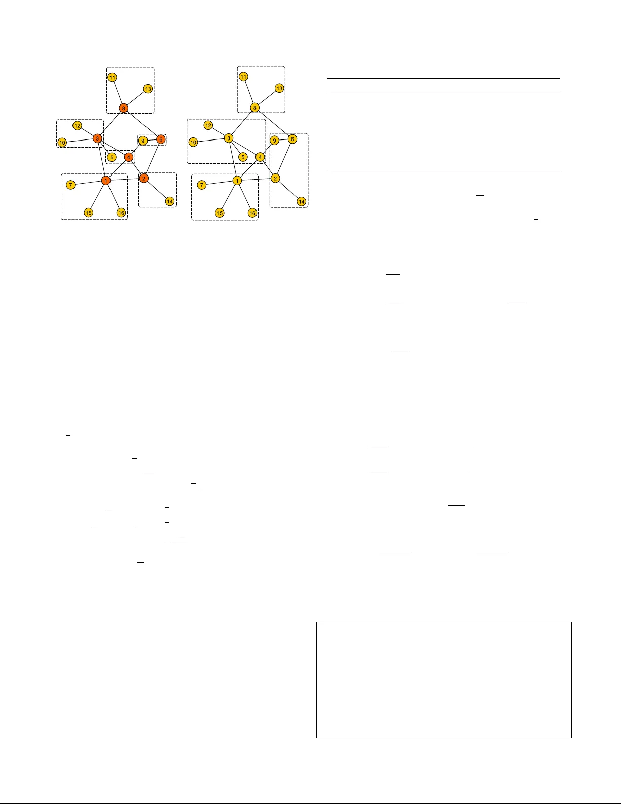
Finding Community Structure with Performance Guarantees in Comple x Networks Thang N. Dinh and My T . Thai Computer & Information Science & Engineering Univ ersity of Florida, Gainesville, FL, 32611, Email: { tdinh,mythai } @cise.ufl.edu Abstract —Many networks including social networks, computer networks, and biological networks are found to divide naturally into communities of densely connected individuals. Finding com- munity structure is one of fundamental pr oblems in network science. Since Newman’ s suggestion of using modularity as a measure to qualify the goodness of community structures, many efficient methods to maximize modularity hav e been proposed but without a guarantee of optimality . In this paper , we propose two polynomial-time algorithms to the modularity maximization problem with theoretical performance guarantees. The first algorithm comes with a priori guarantee that the modularity of f ound community structur e is within a constant factor of the optimal modularity when the network has the power -law degree distribution. Despite being mainly of theoretical interest, to our best knowledge, this is the first approximation algorithm for finding community structure in networks. In our second algorithm, we propose a sparse metric , a substantially faster linear programming method for maximizing modularity and apply a rounding technique based on this sparse metric with a posteriori approximation guarantee . Our experiments show that the r ounding algorithm returns the optimal solutions in most cases and are very scalable, that is, it can run on a network of a few thousand nodes whereas the LP solution in the literature only ran on a network of at most 235 nodes. I . I N T R O D UC T I O N Many complex systems of interest such as the Internet, social, and biological relations, can be represented as net- works consisting a set of nodes which are connected by edges between them. Research in a number of academic fields has uncov ered unexpected structural properties of com- plex networks including small-world phenomenon [1], power - law degree distrib ution [2], and the e xistence of community structure [3] where nodes are naturally clustered into tightly connected modules, also kno wn as communities, with only sparser connections between them. The detection of community structures in networks is an important problem that has drawn an enormous amount of research effort [4]. A huge benefit of identifying community structure is that one can infer semantic attributes for different communities. For example in social networks, the attributes for a community can be common interest or location, and for metabolic networks the attrib ute could be a common function. Moreov er , the relativ e independence among dif ferent commu- nities allows the examining of each community individually , and an analysis of network at a higher-le vel of structure. There are a wide variety of definitions for communities. In general, definitions can be classified into two main categories: local definitions and global definitions . In local definitions, only the group of nodes and its immediate neighborhood are considered, ignoring the rest of the network. For example, communities can be defined as maximal cliques , quasi-cliques , k - ple xes . The most famous definitions in this category are notions of str ong community , where each node has more neigh- bors inside than outside the community , and weak community , where the total number of inner edges must be at least half of the number of outgoing edges. In global definitions, communities can be only recognized by analyzing the network as a whole. This type of defini- tions is especially suitable when the next phase after the community detection is to optimize a global quantity , for example, minimizing the inter-group communication cost. The most widely-used quantity function in the global category is Newman’ s modularity which is defined as the number of edges falling within communities minuses the expected number in an equiv alent network with edges placed at random [5]. A higher value of modularity , a better community structure. Thus, identifying a good community structure of a giv en network becomes finding a partition of networks so as to maximize the modularity of this partition, called modularity maximization problem. Since the introduction of modularity , maximizing modular- ity has become primal approaches to detect community struc- ture. Numerous computational methods have been proposed, based on agglomerative hierarchical clustering [6], simulated annealing [7], genetic search [8], extremal optimization [9], spectral clustering [10], multilevel partitioning [11], and many others. For a comprehensiv e view of community detection methods, we refer to an excellent survey of S. Fortunato and C. Castellano [4]. Unfortunately , Brandes et al. [12] hav e shown that modu- larity maximization is an NP-hard problem, thereby denying the existence of polynomial-time algorithms to find optimal solutions. Thus, it is desirable to design polynomial-time approximation algorithms to find partitioning with a theoretical performance guarantee on the modularity values. In contrary to the vast amount of work on maximizing modularity , the only known polynomial-time approach to find a good community structure with guarantees is due to G. Ag ar- wal and D. Kempe [13] in which they rounded the fractional solution of a linear programming (LP). The value obtained by the LP is an upper bound on the maximum achiev able modularity . Thus, their approach provide a posteriori guarantee on the error bound. In fact, the modularity values found by their approach are optimal for many network instances comparing with the optimal modularity values provided by expensi ve exact algorithms in [14]. The main drawback of the approach is the large LP formulation that consumes both time and memory resources. As shown in their paper , the approach can only be used on the networks of up to 235 nodes. Secondly , while the approach performs well on all considered networks, it does not promise any priori guarantees as pro vided by appr oximation algorithms . In this paper , we address the main drawback of the rounding LP approach by introducing an improv ed formulation, called sparse metric . W e sho w that our ne w technique substantially reduces the time and memory requirements both theoretically and experimentally without any trade-off on the quality of the solution. The size of solved network instances raises from hundred to sev eral thousand nodes while the running time on the medium-instances are sped up from 10 to 150 times. Our second contribution is an approximation algorithm that finds a community structure in networks with modularity values within a constant factor of the optimum when the considered networks hav e power-la w degree distrib utions. T o our best kno wledge, it is the first approximation algorithm for finding community structure in networks. The algorithm is not only of theoretical interest, but also establish a connection between the power-la w degree distribution properties and the presence of community structure in complex networks. Since community structure are often observed together with the power -law property , studying the community structure detec- tion under power -law network models is of great important. Organization. W e present definitions and notions in Section II. W e propose in Section III the sparse metric technique to efficiently maximize modularity via rounding a linear pro- gramming. An approximation algorithm for networks with the power -law degree distrib ution (so-called power -law networks) is introduced in Section IV. W e show experimental results for the sparse metric in Section V to illustrate the time efficienc y over the previous approach. Finally , in Section VI we summarize our results and discuss on limitation of modularity as well as the corresponding resolution. I I . P R E L I M I N A R I E S A network can be represented as an undirected graph G = ( V , E ) consisting of n = | V | nodes and m = | E | edges. The adjacency matrix of G is denoted by A = ( A i,j ) , where A i,j = A j,i = 1 if i and j share an edge and A i,j = A j,i = 0 otherwise. A modularity maximization problem asks us to identify a community structure C = { C 1 , C 2 , . . . , C k } of a given graph where each disjoint subsets C i are called communities and S k i =1 C i = V so as to maximize the modularity of C . Note that k is not a pre-defined value. The modularity [10] of C is the fraction of the edges that fall within the given communities minus the expected number of such fraction if edges were distributed at random. The randomization of the edges is done so as to preserve the degree of each verte x. If nodes i and j hav e degrees d i and d j , then the expected number of edges falling between i and j is d i d j 2 m . Thus, the modularity , denoted Q , is then Q ( C ) = 1 2 m X i,j ( A i,j − d i d j 2 m ) δ ij (1) where δ ij = ( 1 , if i, j are in the same communities 0 , otherwise . . W e also define modularity matrix B [10] as B ij = A ij − d i d j 2 m . W e note that each ro w and column of B sum up to zero, hence, B always has the vector (1 , 1 , 1 , . . . ) as one of its eigen vectors. The same property is also known for the network Laplacian matrix L = D − A , where D is diagonal matrix with the i th entry to be d i . Laplacian matrix L is widely-used in spectral methods for the graph partitioning that is closely related to our community detection problem. W e note that the major difference between the modularity matrix and the Laplacian matrix is that L is positi ve-definite while B is indefinite. As a consequence, while approximation algorithms for the graph partitioning problem using Laplacian matrix L are available, it is not known if such algorithms are possible for the modularity maximization problem. I I I . L I N E A R P R O G R A M M I N G B A S E D A L G O R I T H M A. The Linear Pr ogram and The Rounding The modularity maximization problem can be formulated as an Integer Linear Programming (ILP). The linear program has one variable d i,j for each pair ( i, j ) of vertices to represent the “distance” between i and j i.e. d i,j = ( 0 if i and j are in the same community 1 otherwise . In other words, d i,j is equiv alent to 1 − δ i,j in the definition (1) of modularity . Thus, the objectiv e function to be maximized can be written as X i,j B i,j (1 − d i,j ) . W e note that there should be no confusion between d i,j the variable representing the distance between vertices i and j and constant d i (or d j ), the degree of node i (or j ). The ILP to maximize modularity (IP complete ) is as follows maximize 1 2 m X i,j B i,j (1 − d i,j ) (2) subject to d i,j + d j,k − d i,k ≥ 0 , ∀ i < j < k (3) d i,j − d j,k + d i,k ≥ 0 , ∀ i < j < k (4) − d i,j + d j,k + d i,k ≥ 0 , ∀ i < j < k (5) d i,j ∈ [0 , 1] , i, j ∈ [1 ..n ] , (6) Constraints (3), (4), and (5) are well-known triangle inequal- ities that guarantee the values of d i,j are consistent to each other . They imply the follo wing transiti vity: if i and j are in the same community and j and k are in the same community , then so are i and k . By definition, d i,i = 0 ∀ i and can be remov ed from the ILP for simplification. T o avoid solving ILP , that is also NP-hard, we instead solve the LP relaxation of the ILP , obtained by replacing the constraints d i,j ∈ { 0 , 1 } by d i,j ∈ [0 , 1] . W e shall refer to the IP described above as IP complete and its relaxation as LP complete . If the optimal solution of this relaxation is an integral solution, which is v ery often the case [14], we ha ve a partition with the maximum modularity . Otherwise, we resort on rounding the fractional solution and use the value of the objectiv e as an upper-bound that enables us to lower -bound the gap between the rounded solution and the optimal integral solution. G. Agarwal and D. Kempe [13] use a simple rounding algorithm proposed by Charikar et al. [15] for the correlation clustering problem [16]. The values of d i,j are interpreted as a metric “distance” between vertices. The algorithm repeatedly groups all v ertices that are close by to a v ertex into a community . The final community structure are then refined by a Kernighan-Lin [17] based local search method. Since the rounding phase is comparatively simple, the burden of both time and memory comes from solving the large LP relaxation. The LP has  n 2  variables and 3  n 3  = θ ( n 3 ) constraints that is about half a million constraints for a network of 100 vertices, thereby limiting the the size of networks to few hundred nodes. Thus, there is a need to achieve the same guarantees with smaller resource requirements. By combining mathematical approach with combinatorial techniques, we achiev e this goal in next subsection. B. The Sparse Metric In this subsection, we devise an improv ed LP formulation for the modularity maximization problem with much fewer number of constraints while getting the same guarantees on the performance. Instead of using 3  n 3  triangle inequalities to ensure that d i,j is a metric (or pseudo-metric as defined later), we show that only a compact subset of inequalities, so-called sparse metric , are sufficient to obtain the same fractional optimal solution. A function d is a pseudo-metric if d ( i, j ) = d i,j satisfy the following conditions: 1) d ( i, j ) ≥ 0 (non-negati vity) 2) d ( i, i ) = 0 (and possibly d ( i, j ) = 0 for some distinct values i 6 = j ) 3) d ( i, j ) = d ( j, i ) (symmetry) 4) d ( i, j ) ≤ d ( i, k ) + d ( k, j ) (transitivity). It is clear that d is an feasible solution of LP complete if and only if d is a pseudo-metric within the interval [0 , 1] . Our new linear programming with the Sparse Metric tech- nique, denoted by IP sparse , is as follows: maximize − 1 2 m X i,j B i,j d i,j (7) subject to d i,k + d k,j ≥ d i,j k ∈ N ( i, j ) (8) d i,j ∈ { 0 , 1 } , (9) The objectiv e can be simplified to − 1 2 m X i,j B i,j d i,j since X i,j B i,j = 0 . Let N ( i ) and N ( j ) denote the set of neighbors of i and j , respectiv ely . The set N ( i, j ) is defined as the union of neighbors of i and j N ( i, j ) = N ( i ) ∪ N ( j ) − { i, j } Therefore, the total number of constraints in the formula is upper bounded by X i P i,j d i,j (contradiction). I V . A P P R OX I M A T I O N A L G O R I T H M S F O R M A X I M I Z I N G M O D U L A R I T Y I N P OW E R - L AW N E T W O R K S This section presents approximation algorithms for the mod- ularity maximization problem in power-la w networks. A factor ρ approximation algorithm for a maximization problem, find in polynomial- time a solution with the value no less than ρ times the value of an optimal solution. Approximation algorithms are being used for problems where exact polynomial-time algorithms are too expensiv e and in many cases, they can yield valuable insights to the problem. W e make a detour to focus on the problem of modularity maximization in division of the network into just two com- munities. The maximum modularity v alue of the di vision into two communities are shown to “close” to the best possible modularity . Thus, an approximation algorithm for the division into two communities problem also yields an approximation algorithm for the modularity maximization problem. A. Division into k Communities Let Q k be the maximal modularity obtained by a division of the network into exact k communities. W e also denote Q + k = max k i =1 Q i and Q opt = Q + n , the best possible modularity over all possible di visions. Let δ opt be a community structure with the maximum modularity Q opt . Pr oposition 2: Q 1 = 0 and Q n = − P i d 2 i 4 m 2 . Lemma 1: Q + k ≥ (1 − 1 k ) Q opt Pr oof: If δ opt has at most k communities, than we have Q + k = Q opt . Otherwise δ opt has more than k communities. W e can rewrite the modularity as Q opt = 1 2 m X δ opt ij =1 B ij Construct a k -division of the network by randomly assigning communities in δ opt into one of k new “ super ” communities. Let δ k denote the obtained partitioning. If δ opt ij = 1 , then δ k ij = 1 i.e. all within intra-communities pairs remain within new “super” communities. All pairs ( i, j ) with δ opt ij = 0 (inter-community pairs) become intra-communities pairs with probability 1 /k . Hence, the contribution of a pair ( i, j ) with δ opt ij = 0 to the e xpected modularity is 1 k B ij . Hence, the expected modularity of the k -di vision by randomly grouping communities will be Q E = 1 2 m  X δ opt ij =1 B i,j + 1 k X δ opt i,j =0 B i,j  = 1 2 m  1 − 1 k  X δ opt i,j =1 B i,j =  1 − 1 k  Q opt In the second step, we have used the equality P ij B i,j = 0 or equiv alently P δ opt i,j =1 B i,j = − P δ opt i,j B i,j . Therefore, we hav e Q + k ≥ Q E =  1 − 1 k  Q opt . It follows from Lemma 1 that an approximation algorithm with a factor ρ for maximizing Q 2 will also be an approxima- tion with a factor 2 ρ to the modularity maximization problem. For a division of the network into two groups define x i = ( 1 , if i belong to community 1 − 1 , if i belong to community 2 . W e can write the modularity for the di vision into two communities as Q = 1 4 m X i,j B i,j ( x i x j + 1) = 1 4 m X i,j B i,j x i x j = 1 4 m x T B x Hence, the division into two communities is a special case of the maximizing quadratic program problem i.e. the problem of finding a vector x ∈ {− 1 , 1 } n such that x T B x is maximized. The following results was due to M. Charikar et al. [15] and Nesterov e et al. [20]. Theor em 3: [15] Giv en an arbitrary matrix A , whose diagonal elements are nonnegati ve, the problem of finding x ∈ {− 1 , 1 } n such that x T B x is maximized can be approxi- mated within O (log n ) . In case B is positiv e definite, the ratio can be improv ed to π 2 [20]. Unfortunately , the matrix B is not positive definite. Even worse, the main diagonal contains all negati ve entries as the i th entry is − d 2 i 4 m 2 . Hence, we cannot directly apply abov e results for the division into two communities problem. B. P ower-law Networks Complex networks including social, biological, and technol- ogy networks display a non-tri vial topological feature: their degree sequences can be well-approximated by a power -law distribution [5]. At the same time they exhibit modular prop- erty i.e. the existence of naturally division into communities. W e establish the connection between the po wer-la w degree distribution property and the modular property , stating that whenev er a network ha ve power -law degree distribution, there is presence of communities in the network with a significant modularity . W e use the well-known P ( α, β ) model by F . Chung and L. Lu [21] for power -law networks in which there are y vertices of degree x , where x and y satisfy log y = α − β log x . In other words, |{ v : d ( v ) = x }| = y = e α x β (a) Following algorithm (b) Optimal community structure Fig. 2: On the left, a community structure found by Following Algorithm in Theorem 4 when d 0 = 2 . Each rounded square represents a community . and followees are in the darker color . The modularity is 0.325 i.e. 87% of the optimal modularity , 0.374. On the right, the optimal community structure found by solving IP sparse . Basically , α is the logarithm of the size of the graph ( n = e α ) and β is the log-log growth rate of the graph. While the scale of the network depends on α , β decides the connection pattern and many other important characterizations of the network. Dif ferent networks at different scales with same β often exhibit same characteristics. For instance, the larger β , the sparser and the more “power -law” the network is. Hence, β is regarded as a constant in P ( α, β ) model. In P ( α, β ) model, the maximum degree in a P ( α , β ) graph is e α β . The number of vertices and edges are n = e α β X x =1 e α x β ≈        ζ ( β ) e α if β > 1 αe α if β = 1 e α β 1 − β if β < 1 , m = 1 2 e α β X x =1 x e α x β ≈        1 2 ζ ( β − 1) e α if β > 2 1 4 αe α if β = 2 1 2 e 2 α β 2 − β if β < 2 (11) where ζ ( β ) = P ∞ i =1 1 i β is the Riemann Zeta function. W ithout affecting the conclusions, we will simply use real number instead of rounding down to integers. The error terms can be easily bounded and are sufficiently small in our proofs. Most real-world networks hav e the log-log growth rate β between 2 and 3 . For examples, scientific collaboration networks with 2 . 1 < β < 2 . 45 [22], W ord W ide W eb with β for in-degree and out-degree of 2 . 1 and 2 . 45 , respectiv ely [23]; Internet at router and intra-domain lev el with β = 2 . 48 and so on. No power-la w networks with β < 1 have been observed. One of the reason is that when β < 1 , the number of edges m = Ω( n 2 ) i.e. the network is not “scale-free”. Theor em 4: There is an O (log n ) approximation algorithm for the modularity maximization problem in power -law net- works with the log-log growth rate β > 1 . If β > 2 , the T ABLE I: Order and size of network instances Problem ID Name Nodes n Edges m 1 Zachary’ s karate club 34 78 2 Dolphin’ s social network 62 159 3 Les Miserables 77 254 4 Books about US politics 105 441 5 American College Football 115 613 6 US Airport 97 332 2126 7 Electronic Circuit (s838) 512 819 8 Scientific Collaboration 1589 2742 problem can be approximated within a constant approximation factor 2 ζ ( β − 1) , where ζ ( x ) = P ∞ i =1 1 i x is the Riemann Zeta function. Pr oof: From Lemma (1) with k = 2 , we have 1 2 Q opt ≤ Q + 2 . Hence, it is sufficient to approximate Q + 2 within a factor of O (log n ) . W e hav e Q + 2 = 1 4 m max x ∈{− 1 , 1 } n x T B x = 1 4 m max x ∈{− 1 , 1 } n x T B 0 x − n X i =1 d 2 i 8 m 2 , (12) where B 0 is obtained by replacing the diagonal of B with zeros. Let D = P n i =1 d 2 i 8 m 2 , the second term in equation (12). W e can approximate OPT 0 = max x ∈{− 1 , 1 } n x T B 0 x = Q + 2 + D within a factor of O (log n ) by the method in Theorem 3. That means we can find a division of the network into two communities with the modularity is at least c log n OPT 0 − D = c log n ( Q + 2 + D ) − D ≥ c log n Q + 2 − D ≥ c 2 log n Q opt − D where c is an independent constant. If we can show that D = o  1 log n OPT 0  , then we can ap- proximate the maximum modularity within a factor O (log n ) . This is equiv alent to lim n →∞ Q opt D log n = ∞ or lim α →∞ Q opt D log n = ∞ (13) T o sho w (13), we present a linear-time algorithm, called F ollowing , to find a community structure L with a lo wer bound on the modularity . An illustration example for the algorithm is shown in Fig. 2a. Follo wing Algorithm ( Parameter d 0 ∈ N + ) i. Start with all nodes unlabeled ii. Sort nodes in non-decreasing or der of de gr ee iii. F or each unlabeled node v with d v ≤ d 0 , find a neighbor u that is not a follower; set v to follow u i.e. label v “follower” and u “followee”. If many such u exist, select the one with the minimum degree. iv . Label all unlabeled nodes “followee”. v . Put each follo wee and its follo wers into a community . Despite that higher values of d 0 possibly lead to better approximation ratios, it is sufficient for our proof to con- sider only the case d 0 = 1 . That means all leaf nodes will attach to (follow) their neighbors. Assume that for a graph G = ( V , E ) , vertices in V are numbered so that leaf nodes will hav e higher numbering than non-leaf nodes i.e. V = { v 1 , v 2 , . . . , v t , v t +1 , . . . , v n | {z } leaf no des } in which t is the number of non-leaf nodes. For a node v i , i = 1 . . . t , let l i ≤ d i be the number of leaves attached to v i . There will be t communities associated with v 1 , v 2 , . . . , v t , respectiv ely . Since there are e α vertices of degree one, there are at least 1 2 e α edges inside considered communities. Hence, Q ( L ) = e α 2 m − t X i =1 ( d i + l i ) 2 4 m 2 ≥ e α 2 m − n X i =1 4 d 2 i 4 m 2 = e α 2 m − 8 D (14) Since Q opt ≥ Q ( L ) , instead of showing (13), we can show lim α →∞ Q ( L ) D log n = ∞ ⇔ lim α →∞ e α / 2 m D log n = ∞ From the power -law degree distribution in (11): D = e α β X x =1 e α x β x 2 8 m 2 = e α 8 m 2 e α β X x =1 x 2 − β (15) Consider all three cases of β : Case β > 2 : Since x 2 − β < 1 , from equation (11) we have Q ( L ) ≥ e α 2 m − 8 D ≥ 1 ζ ( β − 1) − 4 e α β ζ ( β − 1) 2 e α ≥ 1 2 ζ ( β − 1) (16) Since Q opt ≤ 1 , community structure L approximate the optimum solutions within a constant factor 2 ζ ( β − 1) . Case β = 2 : W e hav e log n < 2 α . Hence, D log n ≤ 2 e α α 2 e 2 α  e α β X x =1 1  2 α = 4 e α/β αe α Thus, lim α →∞ e α / 2 m D log n ≥ lim α →∞ e α 2 e α/β = ∞ Hence, the modularity maximization problem can be approx- imated within a factor O (log n ) in this case. Case 2 > β > 1 : D log n ≤ e α 8 m 2 e α β (3 − β ) e α β X x =1  x e α β  2 − β 1 e α β 2 α ≤ 2 αe α 2 (2 − β ) 2 e 4 α β e α β (3 − β ) Z 1 0 x 2 − β d x ≤ (2 − β ) 2 e α β α 3 − β Therefore, lim α →∞ e α / 2 m D log n ≥ lim α →∞ e α 2 e 2 α/β 2 − β (3 − β ) e α/β α (2 − β ) 2 ≥ lim α →∞ 3 − β α (2 − β ) e α (1 − β − 1 ) = ∞ Hence, the theorem follows. T ABLE II: The modularity obtained by pre vious published methods GN [5], EIG [10], VP [13], LP complete [13], our sparse metric approach LP sparse and the optimal modularity values OPT [14]. The optimal modularity for network 8 (as a whole) has not been known before; we compute it by solving our our IP sparse within only 15 seconds. ID n GN EIG VP LP complete LP sparse OPT 1 34 0.401 0.419 0.420 0.420 0.420 0.420 2 62 0.520 - 0.526 0.529 0.529 0.529 3 77 0.540 - 0.560 0.560 0.529 0.529 4 105 - 0.526 0.527 0.527 0.529 0.529 5 115 0.601 - 0.605 0.605 0.605 0.605 6 332 - - - - 0.368 0.368 7 512 - - - - 0.819 0.819 8 1589 - - - - 0.955 0.955 V . C O M P U TA T I O NA L E X P E R I M E N T S W e present experimental results for our linear programming rounding algorithm in Section III. The LP solver is GUR OBI 4.5, running on a PC computer with Intel 2.93 Ghz processor and 12 GB of RAM. W e e valuate our algorithm on several standard test cases for community structure identification, consisting of real-world networks. The datasets names together with their sizes are are listed in T able I. The largest network consists of 1580 vertices and 2742 edges. All references on datasets can be found in [13] and [14]. T ABLE III: Number of constraints in formulations LP complete used in papper [13] (Constraint h C i ) and the computational time (in seconds) (T ime h C i ) versus number of constraints in our sparse metric formulation LP sparse (Constraint h S i ) and its computational time(T ime h S i ). ID n Constraint h C i Constraint h S i T ime h C i Time h S i 1 34 17,952 1,441 0.21 0.02 2 62 113,460 5,743 3.85 0.11 3 77 219,450 6,415 13.43 0.08 4 105 562,380 30,236 60.40 1.76 5 115 740,715 66,452 106.27 13.98 6 332 18,297,018 226,523 - 197.03 7 512 66,716,160 294,020 - 53.18 8 1589 2,002,263,942 159,423 - 2.94 Since the same rounding procedure are applied on the opti- mal fractional solutions, both LP complete and LP sparse yield the same modularity values. Ho wev er , LP sparse can run on much larger network instances. The modularity of the rounding LP algorithms and other published methods are shown in T able II. The rounding LP algorithm can find optimal solutions ( or within 0.1% of the optimal solutions) in all cases. The source code for our LP algorithm can be obtained upon request. Finally , we compare the number of constraints of the LP formulation used in [13] and our new formulation (LP sparse ) in T able III. Our new formulation contains substantially less constraints, thus can be solved more effecti vely . The old LP formulation cannot be solv ed within the time allo wance (10000 seconds) and the memory av ailability (12 GB) in cases of the network instances 6 to 8. The largest instance of 1589 nodes is solved surprisingly fast, taking under 3 seconds. The reason is due to the presence of leav es (nodes of degree one) and other special motifs that can be efficiently preprocessed with the reduction techniques in [24]. Our new technique substantially reduces the time and mem- ory requirements both theoretically and experimentally without any trade-off on the quality of the solution. The size of solved network instances raises from hundred to several thousand nodes while the running time on the medium-instances are sped up from 10 to 150 times. Thus, the sparse metric technique is a suitable choice when the network has a moderate size and a community structure with performance guarantees is desired. V I . D I S C U S S I O N W e hav e proposed two algorithms for the modularity maximization problem in complex networks. Our algorithms successfully exploit sparseness and po wer-de gree distribu- tion property found in many complex networks to provide performance guarantees on the solutions. On one hand, the algorithms implied in Theorem 4 are the first approximation al- gorithms for maximizing modularity , hence, are of theoretical interest. On the other hand, our sparse metric approach is an efficient method to find optimal or close to optimal community structure for networks of up to thousand nodes. Fortunato and Barthelemy [25] hav e recently shown that in general quality functions of global defintions of community , including modularity , has an intrinsic resolution scale, known as resolution limit. Therefore, they fail to detect communities smaller than a scale, which depends on global attrib utes of networks such as the total size and the degree of connec- tion among communities. Ho we ver , resolution limit can be ov ercome by introducing a scaling parameter λ > 0 into the original modularity formula as independently proposed by Arenas et al. [26] and R. Lambiotte et al. [27]. Q λ ( C ) = 1 2 m X i,j  A i,j − λ d i d j 2 m  δ i,j Our proposed methods work naturally with this extension with little modification. The only changes in the LP formula- tions are in the objecti ve cofficients; the modularity matrix B is replaced with a new “multi-scale” modularity matrix B λ with B λ i,j = A i,j − λ d i d j 2 m . The sparse metric technique still applies and provides the same guarantees as solving the complete LP formulation. In addition, the constant λ does not affect the asymptotic approximation ratios of algorithms in Theorem 4. Our ongoing work is to design an efficient modularity approximation algorithm that both giv es a better approximation ratio and perform well in practice. R E F E R E N C E S [1] D. J. W atts and S. H. Strogatz, “Collective dynamics of ’ small-world’ networks, ” Nature , vol. 393, no. 6684, 1998. [2] A. Barabasi, R. Albert, and H. Jeong, “Scale-free characteristics of random networks: the topology of the world-wide web, ” Physica A , vol. 281, 2000. [3] R. Milo, S. Shen-Orr, S. Itzkovitz, N. Kashtan, D. Chklovskii, and U. Alon, “Network motifs: simple building blocks of complex net- works.” Science (New Y ork, N.Y .) , vol. 298, no. 5594, 2002. [4] S. Fortunato and C. Castellano, “Community structure in graphs, ” Encyclopedia of Complexity and Systems Science , 2008. [5] M. Girvan and M. E. Newman, “Community structure in social and biological networks. ” PNAS , vol. 99, no. 12, 2002. [6] W . H. E. Day and H. Edelsbrunner, “Efficient algorithms for agglomer- ativ e hierarchical clustering methods, ” Journal of Classification , vol. 1, 1984. [7] J. Reichardt and S. Bornholdt, “Statistical mechanics of community detection, ” Phys. Rev . E. , vol. 74, 2006. [8] A. Gog, D. Dumitrescu, and B. Hirsbrunner , “Community detection in complex networks using collaborative evolutionary algorithms, ” in Advances in Artificial Life , ser . LNCS. Springer Berlin / Heidelberg, 2007, vol. 4648. [9] J. Duch and A. Arenas, “Community detection in complex networks using extremal optimization, ” Phys. Rev . E , vol. 72, no. 2, 2005. [10] M. E. J. Newman, “Modularity and community structure in networks, ” Pr oceedings of the National Academy of Sciences , vol. 103, no. 23, 2006. [11] V . D. Blondel, J.-L. Guillaume, R. Lambiotte, and E. Lefebvre, “Fast unfolding of communities in large networks, ” Journal of Statistical Mechanics: Theory and Experiment , vol. 2008, no. 10, 2008. [12] U. Brandes, D. Delling, M. Gaertler, R. Gorke, M. Hoefer, Z. Nikoloski, and D. W agner , “On modularity clustering, ” Knowledge and Data Engineering, IEEE T ransactions on , vol. 20, no. 2, 2008. [13] G. Agarwal and D. K empe, “Modularity-maximizing graph communities via mathematical programming, ” Eur . Phys. J. B , vol. 66, no. 3, 2008. [14] D. Aloise, S. Cafieri, G. Caporossi, P . Hansen, S. Perron, and L. Liberti, “Column generation algorithms for exact modularity maximization in networks. ” Physical Review E - Statistical, Nonlinear and Soft Matter Physics , vol. 82, 2010. [15] M. Charikar and A. W irth, “Maximizing quadratic programs: Extending grothendieck’ s inequality , ” FOCS , 2004. [16] N. Bansal, A. Blum, and S. Chawla, “Correlation clustering, ” in Machine Learning , 2002. [17] B. W . Kemighan and S. Lin, “ An efficient heuristic procedure for partitioning graphs, ” Journal of Classification , 1970. [18] G. Dantzig, R. Fulkerson, and S. Johnson, “Solution of a large-scale trav eling-salesman problem, ” Operations Research , vol. 2, 1954. [19] D. L. Applegate, R. E. Bixby , V . Chvtal, W . Cook, D. G. Espinoza, M. Goycoolea, and K. Helsgaun, “Certification of an optimal tsp tour through 85,900 cities, ” Operations Resear ch Letter s , vol. 37, no. 1, 2009. [20] Y . Nesterove, “Semidefinite relaxation and noncon ve x quadratic opti- mization, ” CORE Discussion Papers 1997044, 1997. [21] W . Aiello, F . Chung, and L. Lu, “ A random graph model for massiv e graphs, ” in STOC ’00 . New Y ork, NY , USA: ACM, 2000. [22] A. L. Barabsi, H. Jeong, Z. Nda, E. Rav asz, A. Schubert, and T . V icsek, “Evolution of the social network of scientific collaborations, ” Physica A: Statistical Mechanics and its Applications , vol. 311, 2002. [23] R. Albert, H. Jeong, and A. Barabasi, “Error and attack tolerance of complex networks, ” Nature , vol. 406, 2000. [24] D. J. F . A. G. S. Arenas, A, “Size reduction of complex networks preserving modularity , ” New J. Phys. , vol. 9, 2007. [25] S. Fortunato and M. Barthlemy , “Resolution limit in community detec- tion, ” Proceedings of the National Academy of Sciences , vol. 104, no. 1, 2007. [26] A. Arenas, A. Fernandez, and S. Gomez, “ Analysis of the structure of complex networks at different resolution levels, ” New J. Phys. , vol. 10, 2008. [Online]. A vailable: doi:10.1088/1367- 2630/10/5/053039 [27] R. Lambiotte, J. C. Delvenne, and M. Barahona, “Laplacian dynamics and multiscale modular structure in networks, ” arXiv , vol. 812, 2008.