A Testing Framework for P Systems

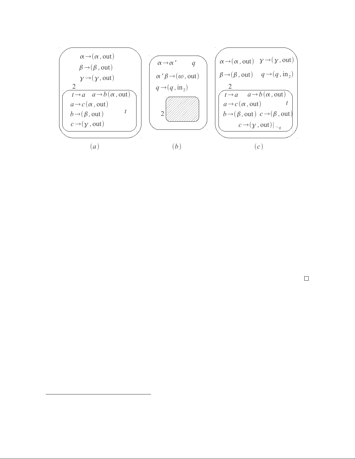
Proceedings of 5th W orkshop on Membrane Computing and Biologically Inspired Process Calculi (MeCBIC 2011) Pages 7–23, 2011. c  R. Barbuti, D. R. Cacciagrano, A. Maggiolo-Schettini P . Milazzo and L. T esei All the rights to the paper remain with the authors. A T esting Framework f or P Systems Roberto Barbuti Dipartimento di Informatica, Univ ersity of Pisa Largo Pontecorv o 3, 56127 Pisa, Italy barbuti@di.unipi.it Diletta Romana Cacciagrano School of Science and T echnology , University of Camerino V ia Madonna delle Carceri 9, 62032 Camerino (MC), Italy diletta.cacciagrano@unicam.it Andrea Maggiolo-Schettini Dipartimento di Informatica, Univ ersity of Pisa Largo Pontecorv o 3, 56127 Pisa, Italy maggiolo@di.unipi.it Paolo Milazzo Dipartimento di Informatica, Univ ersity of Pisa Largo Pontecorv o 3, 56127 Pisa, Italy milazzo@di.unipi.it Luca T esei School of Science and T echnology , University of Camerino V ia Madonna delle Carceri 9, 62032 Camerino (MC), Italy luca.tesei@unicam.it T esting equiv alence was originally defined by De Nicola and Hennessy in a process algebraic set- ting (CCS) with the aim of defining an equiv alence relation between processes being less discrim- inating than bisimulation and with a natural interpretation in the practice of system dev elopment. Finite characterizations of the defined preorders and relations led to the possibility of verification by comparing an implementation with a specification in a setting where systems were seen as black boxes with input and output capabilities, thus ne glecting internal undetectable behaviours. In this paper , we start defining a porting of the well-established testing theory into membrane computing, in order to in vestigate possible benefits in terms of inherited analysis/verification tech- niques and interesting biological applications. P Algebra, a process algebra for describing P Systems, is used as a natural candidate for the porting since it enjo ys the desirable property of being composi- tional and comes with other observational equi valences already defined and studied. W e consider P Systems with multiple membranes, dissolution, promoters and inhibitors. Notions as observable and test are con veniently rephrased in the membrane scenario, where they lack as nativ e notions and have a not so obvious mean. At the same time, concepts as promoters, inhibitors, membrane inclusion and dissolution are emphasized and exploited in the attempt of realizing a testing machinery able to formalize several features, which are proper of membranes and, as a consequence, worth being highlighted as basic observ ables for P Systems. The new testing semantics frame work inherits from the original one the ability to define qualitati ve system properties. Moreov er , it results to be suitable also to express quantitative aspects, a feature which turns out to be very useful for the biological domain and, at the same time, puts in e vidence an expected high expressi ve power of the framew ork itself. 1 Intr oduction Membrane computing, the research field initiated by Gheorghe P ˘ aun [22, 20], aims to define compu- tational models, called P Systems , which are inspired by the behaviour and structure of the living cell. Since its introduction, the P System model has been intensiv ely studied and dev eloped: many v ariants of membrane systems hav e been proposed and regular collecti v e volumes are annually edited. The most in v estigated membrane computing topics are related to the computational power of different v ariants, their capabilities to solve hard problems, decidability , complexity aspects and hierarchies of classes of languages produced by these de vices. In the last years, there have also been significant de velopments in using the P systems paradigm for modelling, simulation and formal verification [11]. Although such topics hav e been exercised to different classes of P Systems [3], testing has been quite neglected in this conte xt. 1.1 T esting and P Systems T esting P Systems has been so far considered by using certain cov erage principles. More often the rule coverage is utilised, by taking into account different contexts. Such contexts - typically grammar, automaton and model checking techniques - are described in depth in [14, 15]: - ( Grammar -based methods ) In order to test an implementation dev eloped from a P System spec- ification in a grammar -based method, a test set is b uilt, in a black box manner , as a finite set of sequences containing references to rules. Although there are similarities between context-free grammars utilised in grammar testing and basic P Systems, there are also major differences that pose new problems in defining testing methods and strategies to obtain test sets. Some of the dif ficulties encountered when some grammar-lik e testing procedures are introduced, are related to the hierarchical compartmentalisation of the P System model, parallel beha viour , communication mechanisms, the lack of a non-terminal alphabet and the use of multisets of objects instead of sets of strings. - ( F inite-state machine methods ) Finite state machine-based testing is widely used for software test- ing. It provides very efficient and exhaustiv e testing strategies and well in vestigated methods to generate test sets. In this case it is assumed that a model of the system under test is pro vided in the form of a finite state machine. In the P System model case, such a machine is typically obtained from a partial computation in a P System. A different approach uses a special class of state machines, called X-machines . Gi ven that the relationships between v arious classes of P Systems and these machines are well studied [1] and the X-machine-based testing is well dev eloped, standard techniques for generating test sets based on X-machines can be adapted to the case of P Systems [16]. Specific coverage criteria are defined in the case of finite state machine-based testing. One such criterion, called transition coverag e , aims to produce a test set in such a way that e very single transition of the model is cov ered. - ( Model chec king-based methods ) The generation of different test sets, according to certain cov- erage criteria, can be done by utilising some specific algorithms or by applying some tools that indirectly will generate test sets. Such tools, like model checkers, can be used to verify some general properties of a model and when these are not fulfilled then some counter -examples are produced, which act as test sets in certain circumstances. In the case of P Systems, an encoding based on a Kripke structure associated with the system is provided for model checkers like NuSMV [17] or SPIN [18]. This relies on certain operations defined in [12] and encapsulates the main features of a P System, including maximal parallelism and communication, but within a finite space of values associated with the objects present in the system. The rule coverage principle is expressed by using temporal logics queries av ailable in such con- texts. By negating specific co verage criteria, counter -examples are generated. 8 1.2 Our contribution: a Process Algebra-based testing machinery f or P Systems The community of Process Algebra taught us that the usefulness of formalisms for the description and the analysis of reactiv e systems is closely related to the underlying notion of behavioural equivalence . Such an equiv alence should formally identify beha viours that are informally indistinguishable from each other , and at the same time distinguish between behaviours that are informally different. The authors of [4] go toward such a direction, proposing some observational equiv alences on a suitable algebraic notation of P Systems. One way of determining behavioural equiv alences is by observing the systems we are interested in, experimenting on them, and drawing conclusions about the behaviour of such systems based on what we see, e.g., testing the system. Such an approach has been formalized in the Process Algebra setting by a suitable testing machinery [13], pi voting on a restricted form of conte xt, called observer . The way to exercise (ev aluate) a process on a gi v en observer is done by letting the considered process and the given observer to run in parallel and by looking at the computations which the running test can perform. It is worth noting that internal actions of the process under test do not af fect, but the case in which they lead to di v ergence, the satisfaction of the test: the y are not observable as input or outputs, thus the y cannot be perceiv ed by an external user that is experimenting on the system. This idea is typical of a testing frame work: systems are considered black box es and only observ ables matter in their comparison. This characteristic is imported in the testing notion introduced in this paper . Internal production and migration of objects in the P system under test will not be seen by the observer: only the objects injected into the system by the observer and the objects that are returned from the system to the observer will matter . Another typical characteristic of the testing framework, worth underlining, is that the observer must hav e the ability to force the system under test to follow certain paths among all the possible ones. This is in order to inv estigate, for instance, what the system can do after a quite specific sequence of inputs, or after a predefined sequence of inputs/outputs. In order to guarantee this possibility , and thus giving the equi valence a discriminating power similar to the one in the original setting, in the testing framew ork we introduce in this paper we exploit promoters and inhibitors. W ithout them the intrinsic nature of P system behaviour , in particular maximal parallelism, would have pre vented this central feature, thus in validating the porting. The characteristics discussed above are central in the idea of testing equi valence. Bisimulation- based equiv alences, ev en the weak one, are highly discriminating and do not reflect a practical view of “testing” a system: usually , and this is always the case for biological systems , the whole internal structure/dynamics of the system is not known, but it is required to check bisimulation. The only way to study such systems is to interact with them and analyse what can be observed from experiments, with the means that are av ailable. Along this idea, we start with this work the definition of a testing frame work with the characteristics above, giving initial theoretical results and some simple examples of tests, without any particular biological impact. Ho wever , we intend as future work to in v estigate and e xploit the analogy of the defined notion of testing with biological experiments in order to giv e more e vidence of the biological rele vance of the work. W e can devise, for instance, techniques for experimental planning that could be of great interest for e xperimental biologists, along the same line of the techniques proposed in [2]. In [13], different equiv alence relations (e.g., may and must testing equiv alences) between systems are defined. T wo systems are considered equiv alent if they pass exactly the same set of observers. Such equi valences are further broken down into preorder relations on systems, i.e., relations that are reflexiv e 9 and transiti ve (though not necessarily symmetric). Formally , given a process P and an observer o , - P may o means that there e xists a successful computation from the test P | o (where | is the parallel operator , and successful means that there is a state where the special action ω is enabled); - P must o means that e very maximal computation from the test P | o is successful; - The preorder P ≤ sat Q means that for any observer o , P sat o implies Q sat o , where sat denotes may or must ; - The equi valence P ≈ sat Q means P ≤ sat Q and Q ≤ sat P . In [23] and in [19] a new testing semantics w as proposed to incorporate the f airness notion: the fair - testing (aka should -testing) semantics. In contrast to the classical must -testing (semantics), fair -testing abstracts from certain di ver gences, e.g., infinite loops of τ (in visible) actions. This is achiev ed by stating that the observer o is satisfied if success always remains within reach in the system under observer . In other words, P fair o holds if in ev ery maximal computation from P | o ev ery state can lead to success after finitely many interactions. On the basis of P Algebra , the algebraic notation of P Systems introduced in [4] (see Section 2), we adapt for P Systems the testing machinery defined in [13] (see Section 3). W e introduce the concept of conte xt in case of P Systems expressed as P Algebra terms. Using this concept, we then define what we consider an observer , which is again a P Algebra term with certain characteristics. This leads naturally to the definition of computations of a running test , i.e. a tested system running together with an observer . Then, following the classical definition of [13], we define the success of a running test in the tw o well-kno wn v ersions of may and must 1 . Finally , the testing preorders are introduced, together with the induced equi valence relations. More in detail: - An observer consists of a membrane structure in which the skin membrane contains sev eral mem- branes (with possibly sub-membranes) one of which is a hole, i.e., a place where another fully defined P System can be placed and run. The skin membrane of this tested P System instantiates the hole membrane and becomes a full component of the running test. - P Systems that are observers are distinguished from P Systems that are normal, testable processes similarly to the classical testing approach, where a particular action, called ω , is used to denote the success of a test and, if the running test is able to perform this action, then the computation under consideration is a successful one. Similarly , in our framework this is easily translated introducing a fresh, particular object ω that, when sent out of the skin membrane of the running test, denotes the success of the computation. - As usual in testing frameworks, we consider only the behaviours of the running test in which no output is produced (this corresponds to considering only in visible action (e.g., τ ) computations in a CCS-like Process Algebra). This is needed to explore all possible behaviours of the tested system while running together with the observer . An important result consists of the fact that, differently from the original testing semantics frame- work, the one proposed here for P Systems results to be suitable to define both qualitati ve and (abo ve all) quantitative system properties. This is mainly because the formalism of P system is expressiv e enough to express both qualitati ve and quantitati ve aspects. Howe ver , these features are crucial for the biological domain. In Section 4, we put quantitati ve capabilities in e vidence defining e xamples of quantitati v e tests, both concerning time and number of indi viduals, of a system modelling a population of individuals that 1 In this paper we do not consider fair testing. 10 can reproduce both se xually and asexually . Note that these examples are to be intended only as explana- tion of the concepts introduced in the paper and not as examples of verifications in the model-checking style. The main direction of continuing this work towards verification is to find finite characterizations of the resulting testing equi valence, possibly with respect to suitable classes of observ ers, and thus using them to compare the expected beha viour of a finite state system with its actual behaviour . 2 Backgr ound W e first briefly recall the definition of P Systems [22, 20]. Then, we give the definition of the syntax and the semantics of the P Algebra as it was presented in [4], where a class of P Systems including rule promoters and inhibitors [10] was considered. The original formulation of the P Algebra, without promoters and inhibitors, can be found in [7, 6] that we refer as a more detailed presentation of the semantics. 2.1 P Systems with Promoters and Inhibitors A P System consists of a hierar chy of membranes , each of them containing a multiset of objects , rep- resenting molecules, a set of evolution rules , representing chemical reactions, and possibly other mem- branes. Each ev olution rule consists of two multisets of objects, describing the reactants and the products of the chemical reaction. A rule in a membrane can be applied only to objects in the same membrane. Some objects produced by the rule remain in the same membrane, others are sent out of the membrane, others are sent into the inner membranes (assumed to exist) which are identified by their labels. In the original definition of P Systems, rules are applied with maximal parallelism , namely it cannot happen that a rule is not applied when the objects needed for its triggering are av ailable. Here, we assume that at each step at least one ev olution rule in the whole system is applied, and also that more than one rule and several occurrences of the same rule can be applied at the same step (to different objects). In other words, we assume that at each step a multiset of ev olution rule instances is non-deterministically chosen and applied in each membrane, such that in the whole system at least one rule is applied. This is a general form of parallelism that is better suited than the maximal one to describe events in biological systems. In P Systems with promoters and inhibitors an ev olution rule in a membrane may ha ve some pr omot- ers and some inhibitors . Promoters are objects that are required to be present and inhibitors are objects that are required to be absent in the membrane m in order to enable the application of the rule. Promoters will be denoted simply as objects, namely a , b , c , . . . , while inhibitors will be denoted as objects preceded by a negation symbol, namely ¬ a , ¬ b , ¬ c , . . . . W e denote with D V the set of all possible promoters and inhibitors symbols that can be obtained from an alphabet V , namely D V = V ∪ ¬ V . Gi ven a set of promoter and inhibitor symbols D , we denote with D + and D − the sets of objects containing all the objects occurring in D as promoters and all the objects occurring in D as inhibitors, respectiv ely . W e remark that D + and D − are sets of objects, hence elements on D − will not be preceded by ¬ . Moreover , with ¬ D we denote the set obtained by transform- ing each promoter in D into an inhibitor and vice versa. As an example, if D = { a , ¬ b , ¬ c , d } we hav e D + = { a , d } , D − = { b , c } and ¬ D = {¬ a , b , c , ¬ d } . W e assume that all ev olution rules have the follo wing form, where u , v h , v o , v 1 , . . . , v n are multisets of objects, { l 1 , . . . , l n } is a set of membrane labels in I N, and D is a set of promoters and inhibitors: u → ( v h , here )( v o , out )( v 1 , in l 1 ) . . . ( v n , in l n ) | D . 11 A rule can be applied only if requirements expressed by D are satisfied. When a rule is applied, the multiset of objects u is replaced by v h , multiset v o is sent to the parent membrane, and each v i is sent to inner membrane l i . Promoters are not consumed by the application of the corresponding e volution rule and a single occurrence of a promoter may enable the application of more than one rule in each ev olution step. Similarly , a single occurrence of an inhibitor forbids the application of all the ev olution rules in which it appears. W e assume that the set of promoters and inhibitors D of an ev olution rule does not contain the same object both as a promoter and as an inhibitor , namely D + ∩ D − = ∅ , and that consumed objects u are not mentioned among inhibitors, namely u ∩ D − = ∅ . Definition 1. A P System Π is a tuple ( V , µ , w 1 , . . . , w n , R 1 , . . . , R n ) wher e: • V is an alphabet whose elements ar e called objects ; • µ ⊂ I N × I N is a membrane structure , such that ( l 1 , l 2 ) ∈ µ denotes that the membr ane labelled by l 2 is contained in the membrane labelled by l 1 ; • w j with 1 ≤ j ≤ n are multisets of objects in V associated with the membranes 1 , . . . , n of µ ; • R j with 1 ≤ j ≤ n are finite sets of e volution rules associated with the membr anes 1 , . . . , n of µ . 2.2 The P Algebra: Syntax and Semantics In this section we recall the P Algebr a , the algebraic notation of P Systems we hav e introduced in [7], with slight modifications introduced in [4]. W e assume V to be an alphabet of objects and we adopt the usual string notation to represent multisets of objects in V . For instance, to represent { a , a , b , b , c } we may write either aabbc , or a 2 b 2 c , or ( ab ) 2 c . W e denote with Set ( u ) the support of multiset u , namely the set of all the objects occurring in u . W e denote multiset (and set) union as string concatenation, hence we write u 1 u 2 for u 1 ∪ u 2 . Moreo ver , we shall write u ( a ) for the number of occurrences of a in multiset u . For the sake of legibility , we shall write u → v h v o { v l i }| D for the generic ev olution rule u → ( v h , here )( v o , out )( v 1 , in l 1 ) . . . ( v n , in l n ) | D . The abstract syntax of the P Algebra is defined as follo ws. Definition 2 (P Algebra) . The abstract syntax of membrane contents c, membranes m, and membrane systems ms is given by the following grammar , where l ranges over I N and a over V : c :: = ( ∅ , ∅ )   ( u → v h v o { v l i }| D , ∅ )   ( ∅ , a )   c ∪ c m :: = [ l c ] l ms :: = ms | ms   µ ( m , ms )   F ( m ) A membrane content c represents a pair ( R , u ) , where R is a set of e volution rules and u is a multiset of objects. A membrane content is obtained through the union operation _ ∪ _ from constants representing single ev olution rules and single objects, and can be plugged into a membrane with label l by means of the operation [ l _ ] l of membranes m . Hence, giv en a membrane content c representing the pair ( R , u ) and l ∈ I N, [ l c ] l represents the membrane having l as label, R as ev olution rules and u as objects. Membrane systems ms have the following meaning: ms 1 | ms 2 represents the juxtaposition of ms 1 and ms 2 , µ ( m , ms ) represents the hierarchical composition of m and ms , namely the containment of ms in m , and F ( m ) represents a flat membr ane , namely it states that m does not contain any child membrane. Juxtaposition is used to group sibling membranes, namely membranes all having the same parent in a membrane structure. This operation allows hierarchical composition µ to be defined as a binary operator on a single membrane (the parent) and a juxtaposition of membranes (all the children). 12 Note that ev ery P System has a corresponding membrane system in the P Algebra, and that there exist membrane systems which do not correspond to an y P System. In what follows we will often write [ [ l c ] ] l for F ([ l c ] l ) . W e shall also often write ( R , u ) where R = { r 1 , . . . , r n } is a set of rules and u = o 1 . . . o m a multiset of objects rather than ( r 1 , ∅ ) ∪ . . . ∪ ( r n , ∅ ) ∪ ( ∅ , o 1 ) ∪ . . . ∪ ( ∅ , o m ) . Moreover , we shall often omit parentheses around membrane contents. The semantics of the P Algebra is giv en as a labelled transition system (L TS). The labels of the L TS can be of the follo wing forms: • ( u , v , v 0 , D , I , O ↑ , O ↓ ) , describing a computation step performed by a membrane content c , where: – u is the multiset of objects consumed by the application of e volution rules in c , as it results from the composition, by means of _ ∪ _, of the constants representing these ev olution rules. – v is the multiset of objects in c offered for the application of the ev olution rules, as it results from the composition, by means of _ ∪ _, of the constants representing these objects. When operation [ l _ ] l is applied to c , it is required that v and u coincide. – v 0 is the multiset of objects in c that are not used to apply any ev olution rule and, therefore, are not consumed, as it results from the composition, by means of _ ∪ _, of the constants representing these objects. – D is a set of promoters and inhibitors required to be present and absent, respectiv ely , by the application of ev olution rules in c . More precisely , D − contains all the inhibitors of the applied ev olution rules in c , whereas D + is a subset of the promoters of those rules. Such a subset contains only those objects that are not present in the multiset of objects of c . – I is the multiset of objects received as input from the parent membrane and from the child membranes. – O ↑ is the multiset of objects sent as an output to the parent membrane. – O ↓ is a set of pairs ( l i , v l i ) describing the multiset of objects sent as an output to each child membrane l i . • ( I ↓ , I ↑ , O ↑ , O ↓ , a p p ) , describing a computation step performed by a membrane m , where: I ↓ is a set containing only the pair ( l , I ) where l is the label of m and I is the multiset of objects receiv ed by m as input from the parent membrane, I ↑ is the multisets of objects receiv ed from the child membranes of m , and O ↑ and O ↓ are as in the previous case. Finally , a p p ∈ { 0 , 1 } is equal to 0 if no rule has been applied in m in the described computation step, and it is equal to 1 otherwise. • ( I ↓ , O ↑ , a p p ) , describing a computation step performed by a membrane system ms , where I ↓ , O ↑ and a p p are as in the previous cases. For the sake of legibility , in transitions with labels of the first form we shall write the first four elements of the label under the arrow denoting the transition and the other elements ov er the arro w . Now , L TS transitions are defined through SOS rules [21]. W e giv e here a very short e xplanation of such rules. Please, refer to [7] for more details. W e start by giving in Fig. 1 the transition rules for membrane contents. Rule ( mc 1 n ) describes n simultaneous applications of an ev olution rule for any n ∈ I N. Rule ( mc 2 ) describes the case in which an ev olution rule is not applied because a subset D 0 of the promoters and inhibitors in D it requires to be present and absent, respecti vely , are assumed not to satisfy the requirements. Rules ( mc 3 ) , ( mc 4 ) and ( mc 5 ) describe the transitions performed by membrane contents consisting of a single object and the transitions performed by an empty membrane content. Rule ( u 1 ) describes the behaviour of a union of membrane contents. In this transition rule we use some auxiliary notations. Giv en two sets O ↓ 1 and O ↓ 2 representing two outputs to inner membranes, 13 I ∈ V ∗ n ∈ I N ( u → v h v o { v l i }| D , ∅ ) I , v n o , { ( l i , v n l i ) } − − − − − − − → u n , ∅ , ∅ , D ( u → v h v o { v l i }| D , I v n h ) ( mc 1 n ) I ∈ V ∗ D 0 ⊆ ¬ D D 0 6 = ∅ ( u → v h v o { v l i }| D , ∅ ) I , ∅ , ∅ − − − − − − − → ∅ , ∅ , ∅ , D 0 ( u → v h v o { v l i }| D , I ) ( mc 2 ) I ∈ V ∗ ( ∅ , a ) I , ∅ , ∅ − − − − − − − → ∅ , a , ∅ , ∅ ( ∅ , I ) ( mc 3 ) I ∈ V ∗ ( ∅ , a ) I , ∅ , ∅ − − − − − − − → ∅ , ∅ , a , ∅ ( ∅ , I a ) ( mc 4 ) I ∈ V ∗ ( ∅ , ∅ ) I , ∅ , ∅ − − − − − − − → ∅ , ∅ , ∅ , ∅ ( ∅ , I ) ( mc 5 ) x 1 I 1 , O ↑ 1 , O ↓ 1 − − − − − → u 1 , v 1 , v 0 1 , D 1 y 1 x 2 I 2 , O ↑ 2 , O ↓ 2 − − − − − → u 2 , v 2 , v 0 2 , D 2 y 2 ( D − 1 ∪ D − 2 ) ∩ Set ( v 1 v 0 1 v 2 v 0 2 ) = ∅ D 1 ∩ ¬ D 2 = ∅ D = ( D 1 D 2 ) \ Set ( v 1 v 0 1 v 2 v 0 2 ) x 1 ∪ x 2 I 1 I 2 , O ↑ 1 O ↑ 2 , O ↓ 1 ∪ I N O ↓ 2 − − − − − − − − − − − → u 1 u 2 , v 1 v 2 , v 0 1 v 0 2 , D y 1 ∪ y 2 ( u 1 ) Figure 1: Transition rules for membrane contents and unions of membrane contents. we write O ↓ 1 ∪ I N O ↓ 2 to denote the set { ( l , uv ) | ( l , u ) ∈ O ↓ 1 ∧ ( l , v ) ∈ O ↓ 2 } ∪ { ( l , u ) | ( l , u ) ∈ O ↓ 1 ∧ @ v . ( l , v ) ∈ O ↓ 2 } ∪ { ( l , v ) | ( l , v ) ∈ O ↓ 2 ∧ @ u . ( l , u ) ∈ O ↓ 1 } . In Fig. 2 we giv e transition rules for individual membranes, juxtaposition and hierarchical compo- sition. Note that from the transition label of the membrane content we have no information about the objects that ha ve been produced by the applied evolution rules. Rules ( m 1 ) and ( m 2 ) describe the tran- sitions performed by a membrane with label l . In particular , ( m 1 ) describes the case in which no objects are received as an input from the external membrane, while ( m 2 ) describes the case in which a multiset of objects I 1 6 = ∅ is recei ved. In these rules a p p is set to zero if no ev olution rule is applied ( u = ∅ ), and it is set to one if at least one rule is applied ( u 6 = ∅ ). Rule ( f m 1 ) allo ws us to infer the behaviour of a flat membrane [ [ l c ] ] l = F ([ l c ] l ) from the behaviour of membrane [ l c ] l . Rule ( j ux 1 ) allows us to infer the behaviour of a juxtaposition of two membrane structures from the behaviours of the two structures. Finally , rule ( h 1 ) describes the behaviour of a hierarchical composition of membranes. In this rule we assume l to be an equi v alence relation on sets of pairs ( l , u ) with l ∈ I N and u ∈ V ∗ , such that, gi ven two such sets I 1 and I 2 , then I 1 l I 2 holds if and only if ( I 1 \ { ( l , ∅ ) | l ∈ I N } ) = ( I 2 \ { ( l , ∅ ) | l ∈ I N } ) . In the last two rules a p p is set to one if at least one between a p p 1 and a p p 2 is equal to one, namely a p p = max ( a p p 1 , a p p 2 ) . This means that at least one rule has been applied in the whole composition. W e conclude by defining a system trace as a sequence of internal information giv en by an ex ecution of a P Algebra term. W e assume that the system can send objects out of the outmost membrane, b ut cannot recei ve objects from outside. This requirement corresponds to the fact that in a P System objects cannot be receiv ed by the outmost membrane from the external en vironment. Note that executions containing steps in which no rule is applied, namely those with 0 as last element of the label, are not considered. Definition 3 (T race) . A trace of a membrane system ms with alphabet V is a (possibly infinite) sequence w of outputs such that, for any O ↑ i and ms i with i ∈ I N + 14 x I , O ↑ , O ↓ − − − − → u , u , v 0 , D y a p p = ( 0 if u = ∅ 1 otherwise D + = ∅ [ l x ] l ∅ , I , O ↑ , O ↓ , a p p − − − − − − − − → [ l y ] l ( m 1 ) x I 1 I 2 , O ↑ , O ↓ − − − − − − → u , u , v 0 , D y a p p = ( 0 if u = ∅ 1 otherwise D + = ∅ I 1 6 = ∅ [ l x ] l { ( l , I 1 ) } , I 2 , O ↑ , O ↓ , a p p − − − − − − − − − − − − → [ l y ] l ( m 2 ) x I ↓ , ∅ , O ↑ , ∅ , a p p − − − − − − − − − → y F ( x ) I ↓ , O ↑ , a p p − − − − − − → F ( y ) ( f m 1 ) x 1 I 1 , O ↑ 1 , a p p 1 − − − − − − − → y 1 x 2 I 2 , O ↑ 2 , a p p 2 − − − − − − − → y 2 x 1 | x 2 I 1 I 2 , O ↑ 1 O ↑ 2 , max ( a p p 1 , a p p 2 ) − − − − − − − − − − − − − − − − → y 1 | y 2 ( j ux 1 ) x 1 I ↓ 1 , I ↑ 1 , O ↑ 1 , O ↓ 1 , a p p 1 − − − − − − − − − − → y 1 x 2 I 2 , O ↑ 2 , a p p 2 − − − − − − − → y 2 O ↓ 1 l I 2 O ↑ 2 = I ↑ 1 µ ( x 1 , x 2 ) I ↓ 1 , O ↑ 1 , max ( a p p 1 , a p p 2 ) − − − − − − − − − − − − − → µ ( y 1 , y 2 ) ( h 1 ) Figure 2: Rules for individual membranes and hierarchical composition of membranes • w = O ↑ 1 O ↑ 2 · · · O ↑ n and ms ∅ , O ↑ 1 , 1 − − − − → ms 1 ∅ , O ↑ 2 , 1 − − − − → . . . ∅ , O ↑ n , 1 − − − − → ms n 6 ∅ , O ↑ , 1 − − − − → or • w = O ↑ 1 O ↑ 2 · · · O ↑ n · · · and ms ∅ , O ↑ 1 , 1 − − − − → ms 1 ∅ , O ↑ 2 , 1 − − − − → ms 2 ∅ , O ↑ 3 , 1 − − − − → .... . W e denote with T the set of all traces. 3 T esting framework W e first introduce the concept of context in case of P Systems expressed as P Algebra terms. Using this concept, we then define what we consider an observer , which is again a P Algebra term with certain characteristics. This leads naturally to the definition of computations of a running test, i.e. a tested system running together with an observer . Then, follo wing the classical definition of [13], we define the success of a test in the two well-known versions of may and must . Finally , the testing preorder is introduced, together with the induced equi valence relation. 3.1 Contexts and test satisfaction At a first look, a natural candidate for conte xt of a P System is another P System, which we call observer , consisting of a membrane structure in which the skin membrane contains sev eral membranes (with pos- sibly sub-membranes) one of which is a “hole”, i.e., a place where another fully defined P System can be placed and run. The skin membrane of this tested P System instantiates 2 the “hole” membrane and becomes a full component of the running test . 2 This instantiation process may require some trivial modifications of the tested P System, such as α -conv ersion of the numbers assigned to the skin and inner membranes. 15 Ho wev er , in [6], a result reg arding flattening P Systems in P Algebra is presented. A similar result can be found in [8]. The flattening process of [6] reduces any P System, specified in P Algebra with promoters and inhibitors, into a flat one (i.e., with no internal membranes) that is bisimilar to the original one. The notion of bisimulation is the one, based on computation steps, defined in [7]. These results suggested us to simplify , without loss of generality , the notion of context we are defining. For this reason, instead of considering an observ er of the form µ ( m , ms 1 | ms 2 | · · · | ms n | 2 ) , we will alw ays consider the equi valent observ er µ ( m 0 , 2 ) where m 0 results from the flattening process of µ ( m , ms 1 | ms 2 | · · · | ms n ) . Another ingredient of the testing framework is needed to distinguish formally P Systems that are observers from P Systems that are normal, testable processes. In classical testing a particular action, usually called ω , is used to denote the “success” of a test, that is to say , if the running test is able to perform this action then the computation under consideration is a successful one. This easily translates in our frame work: we introduction a fresh, particular object, ω 6∈ V that, when sent out of the skin membrane of the running test, denotes the “success” of the computation. Definition 4 (Observ er) . Let V be the alphabet of objects and let ω 6∈ V be a particular object. An observer system , or simply a test , is a P Algebr a term of the form µ ( m , 2 ) wher e m is the skin membr ane [ 1 c ] 1 , 2 is an unspecified membrane ms number ed 2 and each rule of m is of the form u → v h ω o { v l 2 }| D . In other wor ds, m communicates with its only child membr ane 2 and can send out only ω objects. Definition 5 (Running test) . Let V be the alphabet of objects and let ω 6∈ V be a particular object. Let µ ( m , 2 ) be an observer system and let ms be term in P Algebra denoting a closed membrane (i.e., of the form F ( − ) or µ ( − , − ) ). The running test is the P Algebr a term µ ( m , ms 0 ) wher e ms 0 is the term ms in which the former skin membrane (number ed 1) is re-labelled in 2 and the other internal membranes numbers are α -converted in or der not to collide with 1 and 2 (the re-labelling of the membrane names of course implies also applying the substitutions to all the r eferences to the membr ane names in the term.) Definition 6 (Computations) . Let µ ( m , ms ) be a running test. A computation c of µ ( m , ms ) is any sequence of the form: • c is finite: µ ( m , ms ) = ms 0 ∅ , ∅ , 1 − − − → ms 1 ∅ , ∅ , 1 − − − → . . . ∅ , ∅ , 1 − − − → ms n 6 ∅ , ∅ , 1 − − − → or • c is infinite: µ ( m , ms ) = ms 0 ∅ , ∅ , 1 − − − → ms 1 ∅ , ∅ , 1 − − − → ms 2 ∅ , ∅ , 1 − − − → .... A computation is called successful if there ar e k ∈ I N and n ∈ I N + such that ms k ∅ , { ω n } , 1 − − − − − → ms k + 1 , i.e., at least a success symbol can be sent out of the skin membrane along the run. A membr ane like ms k , fr om which a transition can be taken that sends out at least one ω object is called success membrane . W e may also write ms k ω − → to indicate that ms k is a success membrane . Note that, as usual in testing frameworks, we consider only the behaviours of the running test in which no output is produced (this corresponds to considering only τ computations in a CCS-lik e Process Algebra). This is needed to explore all possible behaviours of the tested system while running together with the observer . Note that an unsuccessful computation, i.e. one with no success state along it, can be either finite or infinite. In testing theories diverg ence must have a delicate treatment because it can lead to dif ferent testing preorders [13, 9]. For simplicity we port here the original formulation of [13]. Thus, we define a unary predicate ms ↑ meaning that, with respect to success, the “state” ms along a computation is “underdefined” because it leads to a di ver gent computation. 16 Definition 7 (Di ver gence) . Let c be a computation of a running test µ ( m , ms ) . c is diver gent , which we denote by c ⇑ iff: • c is unsuccessful, or • c contains a membrane ms such that ms ↑ and there is not a success membrane ms 0 pr eceding ms in c. W e now hav e all the ingredients to define the success of a test. Follo wing the classical approach, such a definition comes into version: a may satisfaction, weaker , and a must satisfaction, stronger . Definition 8 (Satisfaction of a test) . Let µ ( m , 2 ) be a test and ms be a closed membrane . Then we say: • ms may µ ( m , 2 ) iff ther e exists a computation c of µ ( m , ms ) and k ∈ I N such that c : µ ( m , ms ) = ms 0 ∅ , ∅ , 1 − − − → ms 1 ∅ , ∅ , 1 − − − → · · · ∅ , ∅ , 1 − − − → ms k and ms k ω − → . • ms must µ ( m , 2 ) iff for eac h computation c of µ ( m , ms ) , c : µ ( m , ms ) = ms 0 ∅ , ∅ , 1 − − − → ms 1 ∅ , ∅ , 1 − − − → ms 2 ∅ , ∅ , 1 − − − → · · · the following conditions hold: (i) ther e is n ∈ I N such that ms n ω − → (ii) if ther e is k ∈ I N such that ms k ↑ , then ther e e xists k 0 ≤ k such that ms k 0 ω − → . Note that, in case of must satisfaction, computations can be infinite, but it is required that a success state is present just at the beginning of di ver gence, or before. 3.2 T esting preorders and testing equiv alences Using the definitions of satisfaction of a test, we naturally deri ve preorders between membrane systems. Definition 9. Let ms 1 and ms 2 two closed membrane systems. W e define two relations v m T and v T between closed membrane systems as follows: • ms 1 v m T ms 2 iff for each observer µ ( m , 2 ), ms 1 may µ ( m , 2 ) ⇒ ms 2 may µ ( m , 2 ) • ms 1 v T ms 2 iff for each observer µ ( m , 2 ), ms 1 must µ ( m , 2 ) ⇒ ms 2 must µ ( m , 2 ) Proposition 1. The r elations v m T and v T ar e pr eor ders. Definition 10 (T esting equiv alence) . W e say that ms 1 is may testing equivalent to ms 2 , and write ms 1 ≈ m T ms 2 , iff ms 1 v m T ms 2 and ms 2 v m T ms 1 . Analogously , we say that ms 1 is must testing equivalent to ms 2 , and write ms 1 ≈ T ms 2 , iff ms 1 v T ms 2 and ms 2 v T ms 1 . Since the defined relations are kernels of preorders, it is easy to conclude that they are equiv alence relations. In [7] some equi v alence relations are defined between the terms of P Algebra. Among them, we con- sider bisimulation, denoted by ≈ , and trace equi v alence, denoted by ≈ T r . W e show that the relationships between these two equiv alences with the must testing equiv alence are the same that hold when classical process calculi, as CCS, are considered [13]. Proposition 2. Let ≈ , ≈ T and ≈ T r as above . Then, ≈ ( ≈ T ( ≈ T r . 17     , ou t      , ou t      , ou t  t  a a  b   , ou t  a  c   , ou t  b    , ou t  c    , ou t  t t  a c    , ou t  | ¬ q t c    , ou t     '  '     , ou t  2 2 2  a   b   c  q   q , i n 2  q     , ou t      , ou t      , ou t  q   q , i n 2  a  b   , ou t  a  c   , ou t  b    , ou t  Figure 3: T wo membrane systems, ( a ) and ( c ) , that are trace equi v alent, but not test equi valent, together with the observer ( b ) that distinguishes them. Pr oof. The two set inclusions can be proved rephrasing the argument used for CCS [13]. Regarding the strictness of the inclusions, Figure 3 shows two systems that are trace equi valent, but can be distinguished by the shown observer . Not that both systems perform the set of traces { ∅ ( α )( β ) , ∅ ( α )( γ ) } . Howe ver , considering the must testing, the observer shown in Figure 3 ( b ) is not satisfied by the system ( a ) because in one computation, after α , only γ can be produced, thus that computation is unsuccessful. Con versely , for the other system ( c ) all computations are successful. Note that inhibitors and promoters are used in this settings to select only specific paths in the system. In the classical setting of testing for synchronous calculi this role is played by the parallel operator together with the restriction on observing only τ - computations. Figure 4 shows two systems that are test equiv alent, but not bisimilar . Below each system the graph of possible transitions 3 is depicted, in order to sho w that bisimulation does not hold. 4 Example of testing scenario In this section we model a population of indi viduals that can reproduce both se xually and asexually . W e define different observers to show the expressi veness of the defined testing framew ork. It is worth noting that quantitative aspects of systems can be easily e xpressed. Note that the defined observers are very specific and are intended to only show the capabilities of the framework introduced above. In particular , the y should not be intended as examples of verification, because this analysis is to be done by checking the testing equiv alence between the system and its expected behaviour , modelled as a simpler “specification” P system. Most animal species use sexual reproduction to produce offspring, while a minority of species re- produce asexually by producing clones of the mother . Both strategies have adv antages and weaknesses. 3 For the sake of le gibility , we omit the third field in the transition labels. 18 y  ...     , ou t      , ou t  a  b   , ou t  a  c   , ou t  b    x , ou t  c    y , ou t  a 2  a  x  ... y  ... a 2 x  ... ° ° ° ° ° ° °  ,   ,   ,   ,   ,   ,  x y ° ° °  ,   ,   ,   ,   ,  ° ° °  b  x y a  b   , ou t  b    x , ou t  b    y , ou t      , ou t      , ou t  Figure 4: T wo membrane systems that are test equiv alent, but not bisimilar , together with their graph of transitions. During sexual reproduction genes from two indi viduals are combined in the offspring that receiv es ge- netic material from both parents in volving, in diploid populations, recombination among genes. Recom- bination can break up fav ourable sets of genes accumulated by selection. Moreover , asexual populations composed by only females can reproduce twice as fast in each generation than sexual populations, be- cause there is no need to produce males for ongoing reproduction. Despite its considerable cost, sexual reproduction it is still by far the most frequent mode of repro- duction in vertebrates. Asexual reproduction has only been described in less than 0 . 1% of vertebrate species. In general, it is assumed that sexually reproducing populations harbour more genetic v ariation than ase xually reproducing populations, and a high le vel of genetic v ariation allo ws perpetual adaptation to changing en vironments. Particularly , populations in heterogeneous habitats, threatened by various parasites or under strong competition, hav e been shown to hav e greater genetic variation. For the above reasons a v ariety of species (essentially among in vertebrates) adopted a mixed strategy which tries to combine the adv antages of both methods [24]. In this example we model a simple organism able to reproduce either sexually or asexually . W e consider the individual of the species as diploid with only a locus (gene), thus each genotype is composed by a pair ( a 1 , a 2 ) of alleles which the two chromosomes have for the gene. Moreover , we consider the sex of individuals, thus each of them is represented by a pair of alleles together with the symbol, f or m , of the sex. The rules controlling the evolution of the population are repr oduction rules , either sexual reproduction rules or asexual, and death rules . Each rule has an inhibitor; when the inhibitor is present the rule cannot be applied. Consider a set of alleles (values for the single gene) of k elements { v 1 , v 2 , . . . , v k } . In the follo wing a 1 , a 2 , a 3 , a 4 belong to { v 1 , v 2 , . . . , v k } . The reproduction rules are the following: 1 . a 1 a 2 m a 3 a 4 f → a 1 a 2 m a 3 a 4 f a i a j s | ¬ no _ sex _ r e pr ( i ∈ { 1 , 2 } , j ∈ { 3 , 4 } , s ∈ { m , f } ) 2 . a 1 a 2 f → a 1 a 2 f a 1 a 2 f | ¬ no _ asex _ r e pr 19 Note that each rule has its inhibitor no _ se x _ re pr or no _ asex _ r e pr . The death rules are the following: 3 . a 1 a 2 m → λ | ¬ no _ mal e _ d ea t h 4 . a 1 a 2 f → λ | ¬ no _ f emal e _ d eat h W e add also rules for females and males which simply surviv e, without reproducing or dying: 5 . a 1 a 2 m → a 1 a 2 m | ¬ no _ mal e _ l i f e 6 . a 1 a 2 f → a 1 a 2 f | ¬ no _ f emal e _ l i f e Finally we use a rule for sending out individuals from the membrane in which the population e volv ed. This rule is pr omoted by the promoter send _ out : 7 . a 1 a 2 m → ( a 1 a 2 m , out ) | send _ ou t 8 . a 1 a 2 f → ( a 1 a 2 f , ou t ) | send _ ou t In the following examples, we consider the membrane system defined above as the system under test. In each example we define a specific observer that is meant to test the ev olution forcing certain situations. The observer controls the system by sending into it both the initial individuals and the pro- moters/inhibitors for constraining the population dynamics. Example 1. Let us consider a population in which the possible alleles for the single locus are { 0 , 1 } and an initial population composed by four males of genotype ( 00 ) and four females of genotype ( 01 ) . Let us contr ol the population dynamics by inhibiting both the sexual r epr oduction and the death of females. The observer we define, using the must version, is able to analyse the following pr operty of the system: “After two time units, no female in the population can dif fer fr om the initial ones, and the number of such females is gr eater than or equal to the initial female number .” Note that naturally the tests e xpr ess quantitati ve aspects, both on time and on numbers of individuals. Assume that membrane 1 , i.e. the observer , initially contains the element a and that I nh is the set of all inhibitors, the rules in membr ane 1 ar e the following: 1 0 . a → 1 (( 00 m ) 4 , ( 01 f ) 4 , no_sex_r e pr , no_ f emal e_d eat h , in 2 ) 2 0 . 1 → 2 3 0 . 2 → 3 ( I nh ∪ { send _out } , in 2 ) 4 0 . 3 → 4 5 0 . a 1 a 2 f → f ail ( a 1 6 = 0 ∨ a 1 6 = 1 ) 6 0 . 4 → 5 7 0 . 5 ( 01 f ) 4 → ( ω , out ) | ¬ f ail Rule 1 0 sends into the membrane under test the initial population (four males and four females) and the inhibitors for sexual r epr oduction and death of females. Rule 2 0 waits for a time unit, and, after that, Rule 3 0 sends, during the second step of the populations evolution, all the inhibitors together with the pr omoter send _out . Rule 4 0 waits for a time unit to allow the inner membrane to send out all the individuals. Afterwar ds, Rule 5 0 pr oduces a f ail if a female differ ent fr om the initial ones is pr esent. At the same time Rule 6 0 incr eases the counter . F inally , Rule 7 0 sends out the ω symbol only if f ail is absent. Example 2. Consider the initial population of Example 1, under the same conditions. Again using a must test, we consider the following pr operty: “Given any k ∈ N , we can chec k that it is not possible, in n time units, for all n ∈ [ 1 , k ] , to pr oduce a female differ ent fr om the initial ones.” Note that this 20 pr operty is not a for-all statement: we count until the given k for chec king it. This is of course weaker than chec king the for-all statement. The rules in membrane 1 ar e the following: 1 0 . a → 1 bl ock (( 00 m ) 4 , ( 01 f ) 4 , no_sex_r e pr , no_ f emal e_d eat h , in 2 ) 2 0 . 1 → 2 3 0 . 2 → 3 · · · k 0 . k − 1 → k ( k + 1 ) 0 . bl ock → bl ock | ¬ k ( k + 2 ) 0 . bl ock → 1 0 ( I nh ∪ { send _out } , in 2 ) 1 0 0 . 1 0 → 2 0 2 0 0 . a 1 a 2 f → f ail ( a 1 6 = 0 ∨ a 1 6 = 1 ) 3 0 0 . 2 0 → 3 0 4 0 0 . 3 0 → ( ω , out ) | ¬ f ail Rules fr om 2 0 to k 0 incr ease the counter until k . At each time unit either Rule ( k + 2 ) 0 can be e xecuted, stopping the e volution of the population, or Rule ( k + 1 ) 0 can be fir ed, allowing the population to e volve for one more step. Rule ( k + 1 ) 0 is inhibited by k , thus when the counter r eaches k the evolution must terminate. Rules fr om 1 0 0 to 4 0 0 pr oduce a ω if and only if, in the final populations there ar e only females equal to the initial ones. Example 3. Consider the initial population of Example 1. This time let us consider a may test ex- pr essing the following: “W ithout initial conditions it is possible to have recombination (offspring with differ ent genotypes with r espect to the initial population) after k steps.” The rules ar e the following: 1 0 . a → 1 bl ock (( 00 m ) 4 , ( 01 f ) 4 , in 2 ) 2 0 . 1 → 2 3 0 . 2 → 3 · · · k 0 . k − 1 → k ( k + 1 ) 0 . k → 1 0 ( I nh ∪ { send _out } , in 2 ) 1 0 0 . 1 0 → 2 0 2 0 0 . a 1 a 2 f → ( ω , ou t ) ( a 1 6 = 0 ∨ a 1 6 = 1 ) 2 0 0 . a 1 a 2 m → ( ω , ou t ) ( a 1 6 = 0 ∨ a 1 6 = 1 ) Example 4. Consider again the initial population of Example 1. Let us define a may test expr essing: “By allowing only the asexual repr oduction for k steps, and then allowing only the sexual r epr oduction for the following k steps, it is possible to have recombination in the final population.” F or this example we need the concept of antidote. An antidote is a symbol able to r emove the effect of an inhibitor , usually for an inhibitor x, the antidote is denoted by ant i_x . The effect of an antidote is described by particular rules, the antidote rules, which have the form ant i_x x → λ . In this example we assume that, in the membrane under test, ther e ar e the antidote rules for the inhibitors no_sex_r e pr and 21 no_sex_r e pr . The rules ar e the following: 1 0 . a → 1 bl ock (( 00 m ) 4 , ( 01 f ) 4 , no_sex_r e pr , in 2 ) 2 0 . 1 → 2 · · · k 0 . k − 1 → k ( ant i_no_sex_re pr , no_asex_r e pr , in 2 ) ( k + 1 ) 0 . k → k + 1 ( 2 k ) 0 . 2 k − 1 → 1 0 ( I nh ∪ { send _out } , in 2 ) 1 0 0 . 1 0 → 2 0 2 0 0 . a 1 a 2 f → ( ω , ou t ) ( a 1 6 = 0 ∨ a 1 6 = 1 ) 2 0 0 . a 1 a 2 m → ( ω , ou t ) ( a 1 6 = 0 ∨ a 1 6 = 1 ) 5 Conclusions The testing machinery defined in [13] and the P Algebra proposed in [4] inspired us a suitable Process Algebra-based testing en vironment for P Systems. On the one hand, the new testing en vironment shares with the original one the concepts of observer , running test, successful and unsuccessful computation, testing preorders/equiv alences, allowing us to define qualitative system properties. On the other hand, dif ferently from the original one, it results to be suitable also to express quantitative aspects. Such a feature puts in evidence an expected high expressiv e power of the framework itself, which needs to be formally studied. The natural continuation of this work is to find finite decidable characterizations of testing equiv- alence of finite state P Algebra terms in order to perform verification by comparing a system with its expected behaviour . Moreov er , we plan to extend the testing en vironment also studying a suitable ver - sion of fair testing semantics for P Systems, as well as rephrasing the testing en vironment for Spatial P Systems [5], with the aim of expressing quantitativ e properties in volving spatial information, being crucial in the biological (and not only) domain. On the biological side, we intend to show as future work the potentials of the testing framew ork of having a practical impact, for instance on planning both in-silico and wet-lab e xperiments. Refer ences [1] J. Aguado, T . Balanescu, T . Cowling, M. Gheorghe, M. Holcombe, and F . Ipate. P Systems with Replicated Rewriting and Stream X-machines (Eilenber g Machines). Fundam. Inf. , 49:17–33, January 2002. [2] J. Ahmad, G. Bernot, J. Comet, D. Lime, and O. Roux. Hybrid Modelling and Dynamical Analysis of Gene Regulatory Networks with Delays. ComPlexUs , 3(4):231–251, 2006. [3] O. Andrei, G. Ciobanu, and D. Lucanu. A Rewriting Logic Framework for Operational Semantics of Mem- brane Systems. Theor . Comput. Sci. , 373(3):163–181, 2007. [4] R. Barbuti, A. Maggiolo-Schettini, P . Milazzo, and D. Gruska. A Notion of Biological Diagnosability In- spired by the Notion of Opacity in Systems Security . Fundamenta Informaticae , 102(1):19–34, 2010. [5] R. Barb uti, A. Maggiolo-Schettini, P . Milazzo, G. P ardini, and L. T esei. Spatial P Systems. Natural Comput- ing , 2010. Receiv ed: 26 October 2009 Accepted: 24 February 2010 Published online: 24 March 2010. [6] R. Barbuti, A. Maggiolo-Schettini, P . Milazzo, and S. Tini. A P Systems Flat Form Preserving Step-by-step Behaviour. Fundamenta Informaticae , 87(1):1–34, 2008. [7] R. Barbuti, A. Maggiolo-Schettini, P . Milazzo, and S. T ini. Compositional Semantics and Behavioral Equi v- alences for P Systems. Theor etical Computer Science , 395(1):77–100, 2008. 22 [8] L. Bianco and V . Manca. Encoding-Decoding Transitional Systems for Classes of P systems. In Pr oc. of WMC 2005, 6th International W orkshop on Membrane Computing , number 3850 in LNCS, pages 134–143. Springer-V erlag, 2006. [9] M. Boreale and R. Pugliese. Basic Observables for Processes. Information and Computation , 149(1):77–98, 1999. [10] P . Bottoni, C. Martín-V ide, G. P ˘ aun, and G. Rozenber g. Membrane Systems with Promoters/Inhibitors. Acta Informatica , 38(10):695–720, 2002. [11] G. Ciobanu, M. J. Pérez-Jiménez, and G. Paun, editors. Applications of Membrane Computing . Natural Computing Series. Springer , 2006. [12] Z. Dang, C. Li, O. H. Ibarra, and G. Xie. On the Decidability of Model-checking for P Systems. J. Autom. Lang. Comb . , 11:279–298, January 2006. [13] R. De Nicola and M. Hennessy . T esting Equiv alences for Processes. Theor etical Computer Science , 34(1- 2):83–133, 1984. [14] M. Gheorghe and F . Ipate. On T esting P Systems. In D. Corne, P . Frisco, G. Paun, G. Rozenberg, and A. Salomaa, editors, Membrane Computing , volume 5391 of Lectur e Notes in Computer Science , pages 204–216. 2009. [15] M. Gheorghe and F . Ipate. T esting Based on P Systems - An Overview. In Pr oceedings of the 11th Interna- tional Confer ence on Membrane Computing , CMC’10, pages 3–6, Berlin, Heidelber g, 2010. Springer -V erlag. [16] F . Ipate and M. Gheorghe. T esting Non-deterministic Stream X-machine Models and P systems. Electr on. Notes Theor . Comput. Sci. , 227:113–126, January 2009. [17] F . Ipate, M. Gheorghe, and R. Lefticaru. T est Generation From P systems Using Model Checking. Journal of Logic and Algebr aic Pr ogr amming , 79(6):350–362, 2010. Membrane computing and programming. [18] F . Ipate, R. Lefticaru, and C. T udose. Formal V erification of P Systems using SPIN. International J ournal of F oundations of Computer Science , 22(1):133–142, 2011. [19] V . Natarajan and R. Cleaveland. Div ergence and Fair T esting. In Pr oceedings of the 22nd International Colloquium on Automata, Langua ges and Pr ogramming , ICALP ’95, pages 648–659, 1995. [20] G. P ˇ aun. Membrane Computing. An Intr oduction . Springer-V erlag, 2002. [21] G. D. Plotkin. A Structural Approach to Operational Semantics. J . Log . Algebr . Pro gram. , 60-61:17–139, 2004. [22] G. P ˇ aun and G. Rozenberg. A Guide to Membrane Computing. Theor etical Computer Science , 287(1):73– 100, 2002. [23] A. Rensink and W . V ogler . Fair testing. [24] I. Schön, K. Martens, and P . van Dijk. Lost Sex: The Evolutionary Biology of P arthenogenesis . Springer V erlag, 2009. 23