A review and comparison of strategies for multi-step ahead time series forecasting based on the NN5 forecasting competition

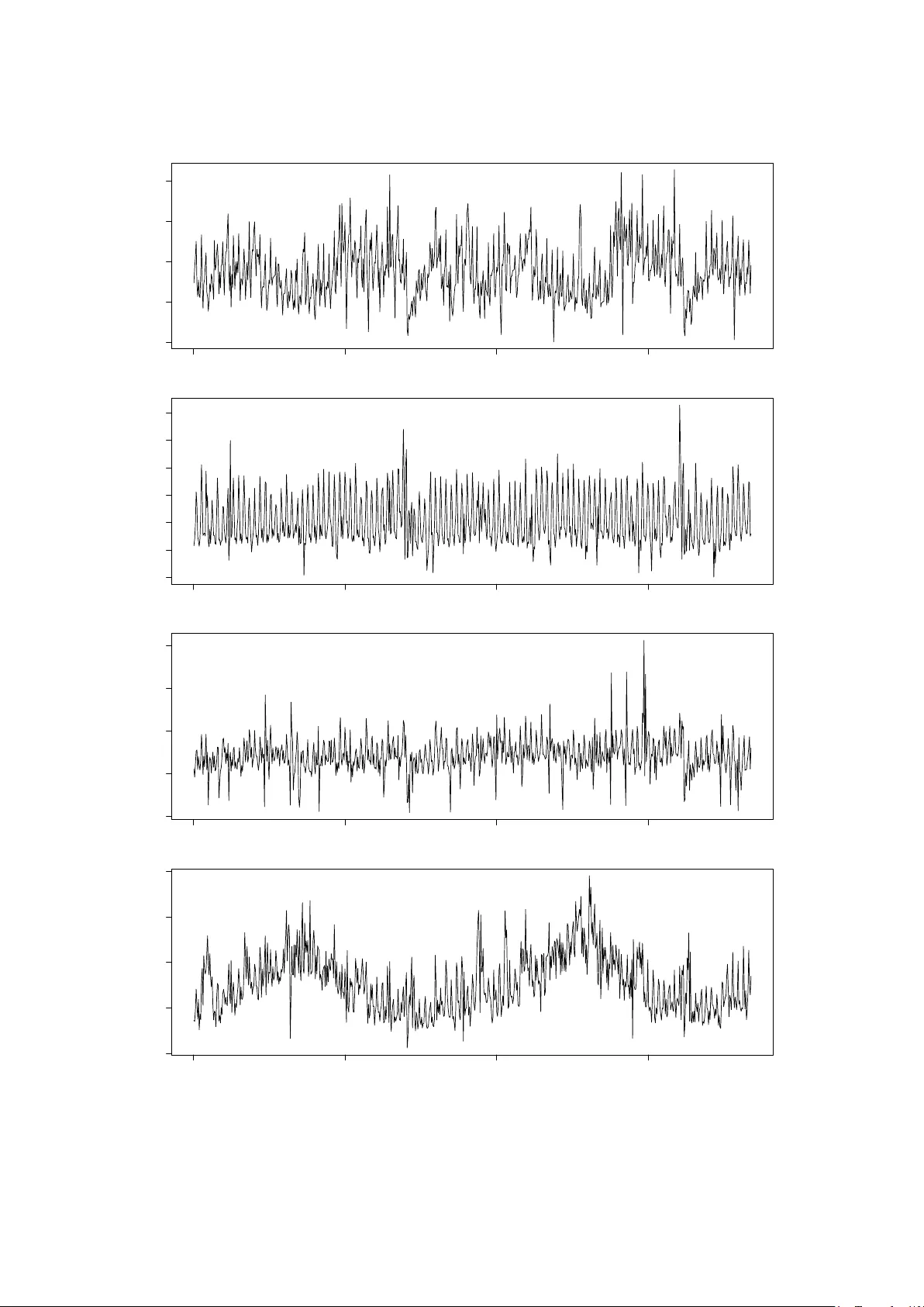
A review and comparison of strategies for m ulti-step ahead time series forecasting based on the NN5 forecasting comp etition Souhaib Ben T aieb a , Gianluca Bon tempi a , Amir A tiya c , An tti Sorjamaa b a Machine L e arning Gr oup, D´ ep artement d’Informatique, F acult´ e des Scienc es, Universit ´ e Libr e de Bruxel les, Belgium b Envir onmental and Industrial Machine L e arning Group, A daptive Informatics R ese ar ch Centr e, Alto o University Scho ol of Scienc e, Finland c F aculty of Engine ering, Cair o University, Giza, Egypt Abstract Multi-step ahead forecasting is still an op en challenge in time series forecasting. Sev eral approac hes that deal with this complex problem ha ve been prop osed in the literature but an extensiv e compar- ison on a large n um b er of tasks is still missing. This paper aims to ﬁll this gap by reviewing existing strategies for m ulti-step ahead forecasting and comparing them in theoretical and practical terms. T o attain suc h an ob jectiv e, we p erformed a large scale comparison of these diﬀerent strategies us- ing a large exp erimen tal b enc hmark (namely the 111 series from the NN5 forecasting comp etition). In addition, we considered the eﬀects of deseasonalization, input v ariable selection, and forecast com bination on these strategies and on multi-step ahead forecasting at large. The follo wing three ﬁndings app ear to b e consisten tly supported by the exp erimental results: Multiple-Output strate- gies are the b est p erforming approaches, deseasonalization leads to uniformly improv ed forecast accuracy , and input selection is more eﬀectiv e when p erformed in conjunction with deseasonaliza- tion. Keywor ds: Time series forecasting, Multi-step ahead forecasting, Long-term forecasting, Strategies of forecasting,, Mac hine Learning, Lazy Learning, NN5 forecasting comp etition, F riedman test. Pr eprint submitte d to Exp ert Systems with Applic ations 11 february 2011 Con ten ts 1 In tro duction 3 2 Strategies for Multi-Step-Ahead Time Series F orecasting 6 2.1 Recursiv e strategy . . . . . . . . . . . . . . . . . . . . . . . . . . . . . . . . . . . . 7 2.2 Direct strategy . . . . . . . . . . . . . . . . . . . . . . . . . . . . . . . . . . . . . . 8 2.3 DirRec strategy . . . . . . . . . . . . . . . . . . . . . . . . . . . . . . . . . . . . . . 8 2.4 MIMO strategy . . . . . . . . . . . . . . . . . . . . . . . . . . . . . . . . . . . . . . 9 2.5 DIRMO strategy . . . . . . . . . . . . . . . . . . . . . . . . . . . . . . . . . . . . . 10 2.6 Comparativ e Analysis . . . . . . . . . . . . . . . . . . . . . . . . . . . . . . . . . . 11 3 Lazy Learning for Time Series F orecasting 15 3.1 Global vs lo cal mo deling for sup ervised learning . . . . . . . . . . . . . . . . . . . . 15 3.2 The Lazy Learning algorithm . . . . . . . . . . . . . . . . . . . . . . . . . . . . . . 16 3.3 Single-Output Lazy Learning algorithm . . . . . . . . . . . . . . . . . . . . . . . . 18 3.4 Multiple-Output Lazy Learning algorithm . . . . . . . . . . . . . . . . . . . . . . . 19 3.5 Mo del selection or mo del av eraging . . . . . . . . . . . . . . . . . . . . . . . . . . . 23 4 Exp erimen tal Setup 24 4.1 Time Series Data . . . . . . . . . . . . . . . . . . . . . . . . . . . . . . . . . . . . . 24 4.2 Metho dology . . . . . . . . . . . . . . . . . . . . . . . . . . . . . . . . . . . . . . . 26 4.2.1 The Compared forecasting strategies . . . . . . . . . . . . . . . . . . . . . . 28 4.2.2 F orecasting p erformance ev aluation . . . . . . . . . . . . . . . . . . . . . . . 30 4.3 Exp erimen tal phases . . . . . . . . . . . . . . . . . . . . . . . . . . . . . . . . . . . 31 4.3.1 Pre-comp etition phase . . . . . . . . . . . . . . . . . . . . . . . . . . . . . . 32 4.3.2 Comp etition phase . . . . . . . . . . . . . . . . . . . . . . . . . . . . . . . . 32 5 Results and discussion 34 5.1 Pre-comp etition results . . . . . . . . . . . . . . . . . . . . . . . . . . . . . . . . . 34 5.2 Comp etition results . . . . . . . . . . . . . . . . . . . . . . . . . . . . . . . . . . . 38 5.3 Discussion . . . . . . . . . . . . . . . . . . . . . . . . . . . . . . . . . . . . . . . . . 43 6 Conclusion 44 1. Introduction Time series forecasting is a gro wing ﬁeld of in terest playing an imp ortan t role in nearly all ﬁelds of science and engineering, suc h as economics, ﬁnance, meteorology and telecommunication (Palit and P op ovic, 2005). Unlik e one-step ahead forecasting, multi-step ahead forecasting tasks are more diﬃcult (Tiao and Tsa y, 1994), since they ha v e to deal with v arious additional complications, lik e accum ulation of errors, reduced accuracy , and increased uncertaint y (W eigend and Gershenfeld, 1994; Sorjamaa et al., 2007). The forecasting domain has b een inﬂuenced, for a long time, b y linear statistical metho ds such as ARIMA models. How e v er, in the late 1970s and early 1980s, it b ecame increasingly clear that linear mo dels are not adapted to man y real applications (Go oijer and Hyndman, 2006). In the same p eriod, sev eral useful nonlinear time series models were prop osed such as the bilinear mo del (Poskitt and T remayne, 1986), the threshold autoregressive mo del (T ong and Lim, 1980; T ong, 1983, 1990) and the autoregressive conditional heteroscedastic (AR CH) mo del (Engle, 1982) (see (Go oijer and Hyndman, 2006) and (Gooijer and Kumar, 1992) for a review). No wada ys, Monte Carlo sim ulation or bo otstrapping metho ds are used to compute nonlinear forecasts. Since no assumptions are made ab out the distribution of the error pro cess, the latter approach is preferred (Clemen ts et al., 2004; Go oijer and Hyndman, 2006). How ev er, the study of nonlinear time series analysis and forecasting is still in its infancy compared to the developmen t of linear time series (Go oijer and Hyndman, 2006). In the last t wo decades, machine learning mo dels ha ve dra wn attention and ha ve established themselv es as serious con tenders to classical statistical mo dels in the forecasting communit y (Ahmed et al., 2010; P alit and Popovic, 2005; Zhang et al., 1998). These models, also called blac k-b o x or data-driv en mo dels (Mitc hell, 1997), are examples of nonparametric nonlinear mo dels whic h use only historical data to learn the sto chastic dep endency b et ween the past and the future. F or in- stance, W erb os found that Artiﬁcial Neural Netw orks (ANNs) outp erforms the classical statistical metho ds such as linear regression and Box-Jenkins approaches (W erb os, 1974, 1988). A similar study has b een conducted b y Lapedes and F arber (Lapedes and F arber, 1987) who conclude that ANNs can b e successfully used for mo deling and forecasting nonlinear time series. Later, others mo dels appeared suc h as decision trees, supp ort vector machines and nearest neighbor regres- sion (Hastie et al., 2009; Alpaydin, 2010). Moreov er, the empirical accuracy of sev eral machine 3 learning mo dels has b een explored in a num b er of forecasting comp etitions under diﬀeren t data conditions (e.g. the NN3, NN5, and the ann ual ESTSP comp etitions (Crone, a,b; Lendasse, 2007, 2008)) creating interesting scien tiﬁc debates in the area of data mining and forecasting (Hand, 2008; Price, 2009; Crone, 2009). In the forecasting comm unity , researchers hav e paid attention to sev eral asp ects of the fore- casting pro cedure such as mo del selection (Aha, 1997; Curry and Morgan, 2006; Anders and Korn, 1999; Chap elle and V apnik, 2000), eﬀect of deseasonalization (Hylleb erg, 1992; Makridakis et al., 1998; Nelson et al., 1999; Zhang and Qi, 2005), forecasts com bination (Bates, J. M. and Granger, C. W. J., 1969; Clemen, 1989; Timmermann, 2006) and man y other critical topics (Go oijer and Hyn- dman, 2006). How ever, approaches for generating m ulti-step ahead forecasts for mac hine learning mo dels did not receive as muc h attention, as p ointed out b y Kline: “ One issue that has had limite d investigation is how to gener ate multiple-step-ahe ad for e c asts ” (Kline, 2004). T o the b est of our knowledge, ﬁv e alternatives (or strategies) ha ve b een prop osed in the litera- ture to tac kle an H -step ahead forecasting task. The R e cursive strategy (W eigend and Gershenfeld, 1994; Sorjamaa et al., 2007; Cheng et al., 2006; Tiao and Tsay, 1994; Kline, 2004; Hamzaebi et al., 2009) iterates, H times, a one-step ahead forecasting mo del to obtain the H forecasts. After estimating the future series v alue, it is fed bac k as an input for the following forecast. In contrast to the previous strategy which use a single mo del, the Dir e ct strategy (W eigend and Gershenfeld, 1994; Sorjamaa et al., 2007; Cheng et al., 2006; Tiao and Tsay, 1994; Kline, 2004; Hamzaebi et al., 2009) estimates a set of H forecasting mo dels, eac h returning a forecast for the i -th v alue ( i ∈ { 1 , . . . , H } ). A com bination of the t wo previous strategies, called DirR e c strategy has b een proposed in (Sor- jamaa and Lendasse, 2006). The idea b ehind this strategy is to com bine asp ects from b oth, the Direct and the Recursiv e strategies. In other w ords, a diﬀerent mo del is used at each step but the appro ximations from previous steps are introduced into the input set. In order to preserve, b et ween the predicted v alues, the sto c hastic dep endency characterizing the time series, the Multi-Input Multi-Output ( MIMO ) strategy has b een in tro duced and analyzed in (Bontempi, 2008; Bontempi and Ben T aieb, 2011; Kline, 2004). Unlike the previous strategies where the models return a scalar v alue, the MIMO strategy returns a vector of future v alues in a single step. 4 The last strategy , called DIRMO (Ben T aieb et al., 2009), aims to preserve the most app ealing asp ects of both the DIRect and miMO strategies. This strategy aims to ﬁnd a trade-oﬀ betw een the prop ert y of preserving the sto c hastic dep endency b et ween the forecasted v alues and the ﬂexibility of the mo deling pro cedure. In the literature, these ﬁve forecasting strategies ha ve b een presented separately , sometimes, using diﬀerent terminologies. The ﬁrst c ontribution of this pap er is to present a thorough uniﬁed review as well as a theoretical comparativ e analysis of the existing strategies for multi-step ahead forecasting. Despite the fact that many studies hav e compared b et w een the diﬀeren t m ulti-step ahead approac hes, the collective outcome of these studies regarding forecasting p erformance has been inconclusiv e. So the mo deler is still left with little guidance as to which strategy to use. F or exam- ple, research from (Bontempi et al., 1999; W eigend et al., 1992) pro vide exp erimental evidence in fa v or of Recursive strategy against Direct strategy . How ever, results from (Zhang and Hutchinson, 1994; Sorjamaa et al., 2007; Hamzaebi et al., 2009) supp ort the fact that the Direct strategy is b etter than the Recursiv e strategy . The work b y (Sorjamaa and Lendasse, 2006) shows that the DirRec strategy gives b etter p erformance than Direct and Recursive strategies. The Direct and Recursiv e strategies ha ve been theoretically and empirically compared in (Atiy a et al., 1999). In this study the authors obtained theoretical and exp erimen tal evidence in fa vor of Direct strategy . Concerning the MIMO strategy , Kline (Kline, 2004) and Cheng et al (Cheng et al., 2006) supp ort the idea that MIMO strategy pro vides worse forecasting performance than Recursive and Direct strategies. Ho w ever, in (Bon tempi, 2008; Bontempi and Ben T aieb, 2011), the comparison b et ween MIMO, Recursive, and Direct was in fav or of MIMO. Finally , (Ben T aieb et al., 2009, 2010) sho w that the DIRMO strategy giv es b etter forecasting results than Direct and MIMO strategies when the parameter controlling the degree of dep endency betw een forecasts is correctly identiﬁed. These previous comparisons hav e b een p erformed with diﬀeren t datasets in diﬀerent conﬁgurations us- ing diﬀerent forecasting methods, suc h as Multiple Linear Regression, Artiﬁcial Neural Net works, Hidden Mark ov Mo dels and Nearest Neigh b ors. All the con tradictory ﬁndings of these studies make it all the more necessary to inv estigate further to ﬁnd the truth concerning the relativ e p erformance of these strategies. The se c ond c on- tribution of this pap er is an exp erimental comparison of the diﬀeren t m ulti-step ahead forecasting 5 strategies on the 111 time series of the NN5 international forecasting competition b enchmark. These time series p ose some of the realistic problems that one usually encoun ters in a t ypical m ulti-step ahead forecasting task, for example the existence of several times series of possibly re- lated dynamics, outliers, missing v alues, and multiple o verlying seasonalities. This exp erimen tal comparison is p erformed for a v ariety of diﬀeren t conﬁgurations (regarding seasonalit y , input se- lection and combination), in order to hav e the comparison as encompassing as can b e. In addition, the methodology used for this experimental comparison is based on the guidelines and recom- mendations adv o cated in some of the metho dological pap ers (Dem ˇ sar, 2006; Garca and Herrera, 2009). In other w ords, the aim of this pap er is not to mak e a comparison of mac hine learning algorithms for forecasting (whic h was already conducted in (Ahmed et al., 2010)) but rather to sho w for a giv en learning algorithm, ho w the choice of the forecasting strategy can sensibly inﬂuence the p erformance of the multi-step ahead forecasts. In this work, w e adopted the Lazy Learning algorithm (Aha, 1997), a particular instance of lo cal learning, whic h has b een successfully applied to many real-w orld forecasting tasks (Sauer, 1994; Bon tempi et al., 1998; McNames, 1998). Last but not least, the pap er prop oses also a Lazy Learning entry to the NN5 forecasting com- p etition (Crone, b). The goal is to assess ho w this mo del fares compared to the other computational in telligence mo dels that w ere prop osed for the comp etition (Bontempi and Ben T aieb, 2011). This will giv e us an idea ab out the p oten tial of this approach. The paper is organized as follo ws. The next section presen ts a review of the diﬀeren t forecasting strategies. Section 3 describ es the Lazy Learning mo del and the asso ciated algorithms for the diﬀeren t forecasting strategies. Section 4 gives a detailed presen tation of the datasets and the metho dology applied for the exp erimen tal comparison. Section 5 presen ts the results and discusses them. Finally , Section 6 gives a summary and concludes the work. 2. Strategies for Multi-Step-Ahead Time Series F orecasting A m ulti-step ahead (also called long-term) time series forecasting task consists of predicting the next H v alues [ y N +1 , . . . , y N + H ] of a historical time series [ y 1 , . . . , y N ] comp osed of N observ ations, where H > 1 denotes the forecasting horizon. This section will ﬁrst giv e a presen tation of the ﬁve forecasting strategies and next, a subsection will b e dev oted to a comparativ e analysis of these strategies in terms of n umber and types of mo dels 6 to learn as w ell as forecasting prop erties. W e will use a common notation where f and F denote the functional dep endency b et ween past and future observ ations, d refers to the embedding dimension (Casdagli et al., 1991) of the time series, that is the num b er of past v alues used to predict future v alues and w represents the term that includes mo deling error, disturbances and/or noise. 2.1. R e cursive str ate gy The oldest and most in tuitive forecasting strategy is the R e cursive (also called Iter ate d or Multi-Stage ) strategy (W eigend and Gershenfeld, 1994; Sorjamaa et al., 2007; Cheng et al., 2006; Tiao and Tsa y, 1994; Kline, 2004; Hamzaebi et al., 2009). In this strategy , a single mo del f is trained to p erform a one-step ahe ad forecast, i.e. y t +1 = f ( y t , . . . , y t − d +1 ) + w , (1) with t ∈ { d, . . . , N − 1 } . When forecasting H steps ahead, w e ﬁrst forecast the ﬁrst step b y applying the model. Sub- sequen tly , we use the v alue just forecasted as part of the input v ariables for forecasting the next step (using the same one-step ahead mo del). W e contin ue in this manner until w e ha ve forecasted the en tire horizon. Let the trained one-step ahead mo del be ˆ f . Then the forecasts are giv en b y: ˆ y N + h =              ˆ f ( y N , . . . , y N − d +1 ) if h = 1 ˆ f ( ˆ y N + h − 1 , . . . , ˆ y N +1 , y N , . . . , y N − d + h ) if h ∈ { 2 , . . . , d } ˆ f ( ˆ y N + h − 1 , . . . , ˆ y N + h − d ) if h ∈ { d + 1 , . . . , H } (2) Dep ending on the noise present in the time series and the forecasting horizon, the recursiv e strategy may suﬀer from low p erformance in m ulti-step ahead forecasting tasks. Indeed, this is esp ecially true if the forecasting horizon h exceeds the em b edding dimension d , as at some p oin t all the inputs are forecasted v alues instead of actual observ ations (Equation 2). The reason for the p oten tial inaccuracy is that the Recursive strategy is sensitiv e to the accum ulation of errors with the forecasting horizon. Errors present in in termediate forecasts will propagate forward as these forecasts are used to determine subsequen t forecasts. 7 In spite of these limitations, the Recursive strategy has b een successfully used to forecast man y real-world time series by using diﬀerent machine learning mo dels, lik e recurrent neural net- w orks (Saad et al., 1998) and nearest-neighbors (McNames, 1998; Bontempi et al., 1999). 2.2. Dir e ct str ate gy The Dir e ct (also called Indep enden t) strategy (W eigend and Gershenfeld, 1994; Sorjamaa et al., 2007; Cheng et al., 2006; Tiao and Tsa y, 1994; Kline, 2004; Hamzaebi et al., 2009) consists of fore- casting each horizon indep endently from the others. In other terms, H mo dels f h are learned (one for eac h horizon) from the time series [ y 1 , . . . , y N ] where y t + h = f h ( y t , . . . , y t − d +1 ) + w , (3) with t ∈ { d, . . . , N − H } and h ∈ { 1 , . . . , H } . The forecasts are obtained b y using the H learned mo dels ˆ f h as follo ws: ˆ y N + h = ˆ f h ( y N , . . . , y N − d +1 ). (4) This implies that the Direct strategy do es not use any appro ximated v alues to compute the forecasts (Equation 4), b eing then immune to the accumulation of errors. How ever, the H mo dels are learned indep enden tly inducing a conditional indep endence of the H forecasts. This aﬀects the forecasting accuracy as it preven ts the strategy from considering complex dep endencies b et ween the v ariables ˆ y N + h (Bon tempi, 2008; Bon tempi and Ben T aieb, 2011; Kline, 2004). F or example consider a case where the b est forecast is a linear or mildly nonlinear trend. The direct metho d could yield a brok en curv e because of the “unco operative” wa y the H forecasts are generated. Also, this strategy demands a large computational time since there are as man y mo dels to learn as the size of the horizon. Diﬀeren t machine learning mo dels hav e b een used to implemen t the Direct strategy for multi- step ahead forecasting tasks, for instance neural netw orks (Kline, 2004), nearest neigh b ors (Sorja- maa et al., 2007) and decision trees (T ran et al., 2009). 2.3. DirR e c str ate gy The DirR e c strategy (Sorjamaa and Lendasse, 2006) com bines the arc hitectures and the prin- ciples underlying the Direct and the Recursive strategies. DirRec computes the forecasts with 8 diﬀeren t mo dels for every horizon (lik e the Direct strategy) and, at eac h time step, it enlarges the set of inputs by adding v ariables corresp onding to the forecasts of the previous step (like the Recursiv e strategy). How ever, note that unlik e the tw o previous strategies, the em b edding size d is not the same for all the horizons. In other terms, the DirRec strategy learns H mo dels f h from the time series [ y 1 , . . . , y N ] where y t + h = f h ( y t + h − 1 , . . . , y t − d +1 ) + w , (5) with t ∈ { d, . . . , N − H } and h ∈ { 1 , . . . , H } . T o obtain the forecasts, the H learned mo dels are used as follows: ˆ y N + h =      ˆ f h ( y N , . . . , y N − d +1 ) if h = 1 ˆ f h ( ˆ y N + h − 1 , . . . , ˆ y N +1 , y N , . . . , y N − d +1 ) if h ∈ { 2 , . . . , H } (6) This strategy outp erformed the Direct and the Recursiv e strategies on t wo real-world time series: San ta F e and P oland Electricit y Load data sets (Sorjamaa and Lendasse, 2006). F ew researc h has b een done regarding this strategy , so there is a need for further ev aluation. 2.4. MIMO str ate gy The three previous strategies (Recursive, Direct and DirRec) may b e considered as Single- Output strategies (Ben T aieb et al., 2010) since they mo del the data as a (m ultiple-input) single- output function (see Equations 2, 4 and 6). The introduction of the Multi-Input Multi-Output (MIMO) strategy (Bontempi, 2008; Bon- tempi and Ben T aieb, 2011) (also called Join t strategy (Kline, 2004)) has been motiv ated b y the need to a v oid the mo deling of single-output mapping, whic h neglects the existence of sto c hastic de- p endencies b et w een future v alues and consequently aﬀects the forecast accuracy (Bon tempi, 2008; Bon tempi and Ben T aieb, 2011). The MIMO strategy learns one m ultiple-output model F from the time series [ y 1 , . . . , y N ] where [ y t + H , . . . , y t +1 ] = F ( y t , . . . , y t − d +1 ) + w , (7) with t ∈ { d, . . . , N − H } , F : R d → R H is a vector-v alued function (Micchelli and P ontil, 2005), and w ∈ R H is a noise v ector with a cov ariance that is not necessarily diagonal (Mat ´ ıas, 2005) . 9 The forecasts are returned in one step b y a multiple-output mo del ˆ F where [ ˆ y t + H , . . . , ˆ y t +1 ] = ˆ F ( y N , . . . , y N − d +1 ). (8) The rationale of the MIMO strategy is to preserve, b et ween the predicted v alues, the sto chastic dep endency characterizing the time series. This strategy av oids the conditional indep endence assumption made b y the Direct strategy as w ell as the accum ulation of errors from whic h plagues the Recursiv e strategy . So far, this strategy has b een successfully applied to sev eral real-world m ulti-step ahead time series forecasting tasks (Bon tempi, 2008; Bontempi and Ben T aieb, 2011; Ben T aieb et al., 2009, 2010). Ho w ever, the need to preserve the sto c hastic dep endencies by using one mo del has a drawbac k as it constrains all the horizons to be forecasted with the same model structure. This constrain t could reduce the ﬂexibilit y of the forecasting approach (Ben T aieb et al., 2009). This was the motiv ation for the in tro duction of a new multiple-output strategy: DIRMO (Ben T aieb et al., 2009, 2010), presen ted next. 2.5. DIRMO str ate gy The DIRMO strategy (Ben T aieb et al., 2009) aims to preserv e the most app ealing asp ects of b oth the DIRect and miMO strategies. T aking a middle approac h, DIRMO forecasts the horizon H in blo c ks, where eac h block is forecasted in a MIMO fashion. Th us, the H -step-ahead forecasting task is decomp osed into n m ultiple-output forecasting tasks ( n = H s ), each with an output of size s ( s ∈ { 1 , . . . , H } ). When the v alue of the parameter s is 1, the n umber of forecasting tasks n is equal to H whic h corresp ond to the Direct strategy . When the v alue of the parameter s is H , the num b er of forecasting tasks n is equal to 1 which corresp ond to the MIMO strategy . There are intermediate conﬁgurations b et ween these tw o extremes dep ending on the v alue of a parameter s . The tuning of the parameter s allows us to improv e the ﬂexibility of the MIMO strategy by calibrating the dimensionality of the outputs (no dep endency in the case s = 1 and maximal dep endency for s = H ). This provides a b eneﬁcial trade oﬀ b et ween the preserving a larger degree of the stochastic dep endency betw een future v alues and ha ving a greater ﬂexibilit y of the predictor. The DIRMO strategy , previously called MISMO strategy (Ben T aieb et al., 2009) (renamed for clarit y reason), learns n mo dels F p from the time series [ y 1 , . . . , y N ] where 10 [ y t + p ∗ s , . . . , y t +( p − 1) ∗ s +1 ] = F p ( y t , . . . , y t − d +1 ) + w , (9) with t ∈ { d, . . . , N − H } , p ∈ { 1 , . . . , n } and F p : R d → R s is a v ector-v alued function if s > 1. The H forecasts are returned by the n learned mo dels as follows: [ ˆ y N + p ∗ s , . . . , ˆ y N +( p − 1) ∗ s +1 ] = ˆ F p ( y N , . . . , y N − d +1 ). (10) The DIRMO strategy has b een successfully applied to t wo forecasting comp etitions: ESTSP’07 (Ben T aieb et al., 2009) and NN3 (Ben T aieb et al., 2010). 2.6. Comp ar ative A nalysis T o summarize, there are ﬁve p ossible forecasting strategies that p erform a m ulti-step ahead forecasting task: R e cursive , Dir e ct , DirR e c , MIMO and DIRMO strategies. Figure 1 sho ws the diﬀeren t forecasting strategies with links indicating their relationships. Recursive Direct MIMO DirRec DIRMO Figure 1: The diﬀerent forecasting strategies with the links sho wing their relationship. As we see, the DirRec strategy is a combination of the Direct and the Recursive strategy , while the DIRMO strategy is a com bination of the Direct and the MIMO strategy . Con tingen t on the selected strategy , a diﬀerent num b er and type of mo dels will b e required. Before presen ting the general comparison of the m ulti-step ahead forecasting strategies, let us highligh t using an example the diﬀerences b et w een the forecasting strategies. Consider a multi-step ahead forecasting task for the time series [ y 1 , . . . , y N ] where the forecasting horizon H is 4. T able 1 shows, for each strategy , the diﬀeren t input sets and forecasting mo dels in v olved in the calculation of the four forecasts [ ˆ y N +1 , . . . , ˆ y N +4 ]. 11 ˆ y N +1 ˆ y N +2 ˆ y N +3 ˆ y N +4 Recursiv e ˆ f ( y N ,...,y N − d +1 ) ˆ f ( ˆ y N +1 ,y N ,...,y N − d +2 ) ˆ f ( ˆ y N +2 , ˆ y N +1 ,...,y N − d +3 ) ˆ f ( ˆ y N +3 , ˆ y N +2 ,...,y N − d +4 ) Direct ˆ f 1 ( y N ,...,y N − d +1 ) ˆ f 2 ( y N ,...,y N − d +1 ) ˆ f 3 ( y N ,...,y N − d +1 ) ˆ f 4 ( y N ,...,y N − d +1 ) DirRec ˆ f 1 ( y N ,...,y N − d +1 ) ˆ f 2 ( ˆ y N +1 ,y N ,...,y N − d +1 ) ˆ f 3 ( ˆ y N +2 , ˆ y N +1 ,...,y N − d +1 ) ˆ f 4 ( ˆ y N +3 , ˆ y N +2 ,...,y N − d +1 ) MIMO ˆ F ( y N ,...,y N − d +1 ) DIRMO ( s = 2) ˆ F 1 ( y N ,...,y N − d +1 ) ˆ F 2 ( y N ,...,y N − d +1 ) T able 1: The diﬀerent forecasting mo dels used b y eac h strategy to obtain the 4 forecasts needed. Let T S O and T M O denote the amount of computational time needed to learn (with a given learning algorithm) a Single-Output mo del and a Multiple-Output mo del, resp ectiv ely . F or a giv en H -step ahead forecasting task, we can see in T able 2 for eac h strategy the num b er and t yp e of mo dels to learn, the size of the output for each mo del as well as the computational time. Num b er of Models Types of mo dels Size of output Computational time Recursiv e 1 SO 1 1 × T S O Direct H SO 1 H × T S O DirRec H SO 1 H × ( T S O + µ ) MIMO 1 MO H 1 × T M O DIRMO H s MO s H s × T M O T able 2: F or eac h forecasting strategy: the num b er and t yp e of mo dels (Single-Output or Multiple- Output) to learn and the size of the output for eac h mo del. Supp ose T M O = T S O + δ , which is a reasonable assumption b ecause learning a mo del with a v ector-v alued output tak es m ore time than learning a mo del with a single-v alued output. This allo ws us to rank the forecasting strategies according to their computation time for training given in T able 2. Indeed, we hav e 1 × T S O | {z } Recur sive < 1 × T M O | {z } M I M O < H s × T M O | {z } DI RM O < H × T S O | {z } Dir ect < H × ( T S O + µ ) | {z } Dir Rec , (11) where w e supp ose that the parameter s of DIRMO is not equal to 1 or H . Note, in one hand, that the time needed to learn a SO mo del of the DirRec strategy equals T S O + µ because the input size of eac h SO task increases at eac h step. On the other hand, if w e need to select the v alue of the parameter s by on some tuning, the DIRMO strategy will take more time and hence will b e the slo west one. 12 In the following, we conclude this section by summarizing the pros and cons of the ﬁve fore- casting strategies as depicted on T able 3. 13 Pros Cons Computational time needed Recursiv e Suitable for noise-free time series (e.g. c haotic) Accum ulation of errors + Direct No accum ulation of errors Conditional indep endence assumption + + ++ DirRec T rade-oﬀ b et ween Direct and Recursiv e Input set gro ws linearly with H + + + + + MIMO No conditional indep endence assumption Reduced ﬂexibilit y: same mo del structure for all the horizons ++ DIRMO T rade-oﬀ b et ween total dep endence and total indep endence of forecasts One additional parameter to estimate + + + T able 3: A Summary of the Pros and Cons of the Diﬀerent Multi-step F orecasting Strategies 14 3. Lazy Learning for Time Series F orecasting Eac h of the forecasting strategies introduced in Section 2 demands the deﬁnition of a sp eciﬁc forecasting model or learning algorithm to estimate either the scalar-v alued function f (see Equa- tions 1, 3 and 5) or the v ector-v alued function F (see Equations 7 and 9) whic h represent the temp oral sto chastic dep endencies. As the goal of the pap er is not to compare forecasting mo d- els (as in (Ahmed et al., 2010)) but rather multi-step ahead forecasting strategies, the choice of a underlying forecasting model is required to setup the experiments. In this paper, w e adopted the Lazy Learning algorithm, whic h is a particular instance of lo cal learning mo dels, since it has b een sho wn to b e particularly eﬀectiv e in time series forecasting tasks (Bontempi et al., 1998; Bon tempi, 1999, 2008; Bon tempi and Ben T aieb, 2011; Ben T aieb et al., 2009, 2010). Next section giv es a general comparison of global models with lo cal mo dels. Section 3.2 presents the Lazy Learning Algorithm in terms of learning properties. Section 3.3 and 3.4 describ e t wo Lazy Learning algorithms for t wo t yp es of learning tasks, namely the Single-Output and Multiple-Output Lazy Learning algorithms. Finally , the a discussion is presented on the mo del combination. 3.1. Glob al vs lo c al mo deling for sup ervise d le arning F orecasting the future v alues of a time series using past observ ations can b e reduced to a sup ervised learning problem or, more precise ly , to a regression problem. Indeed, the time series can b e seen as a dataset made of pairs where the ﬁrst comp onen t, called input, is a past temp oral pattern and the second, called output, is the corresp onding future pattern. Being able to predict the unknown output for a giv en input is equiv alent to forecasting the future v alues giv en the last observ ations of the time series. Glob al mo deling is the typical approach to the sup ervised learning problem. Global mo dels are parametric mo dels that describ e the relationship b et ween the inputs and the output v alues as an analytical function ov er the whole input domain. Examples of global mo dels are linear mo dels (Montgomery et al., 2006), nonlinear statistical regressions (Seb er and Wild, 1989) and Neural Net works (Rumelhart et al., 1986). Another approac h is the divide-and-c onquer mo deling whic h consists in relaxing the global mo deling assumptions by dividing a complex problem in to simpler problems, whose solutions can b e com bined to yield a solution to the original problem (Bontempi, 1999). The divide-and-conquer 15 has evolv ed in t w o diﬀeren t paradigms: the mo dular ar chite ctur es and the lo c al mo deling ap- proac h (Bontempi, 1999). Mo dular te chniques replace a global model with diﬀeren t mo dules co vering diﬀerent parts of the input space. Examples based on this approac h are F uzzy Inference Systems (T ak agi and Sugeno, 1985), Radial Basis F unctions (Mo ody and Dark en, 1989; P oggio and Girosi, 1990), Lo cal Model Net w orks (Murra y-Smith, 1994), T rees (Breiman et al., 1984) and Mixture of Exp erts (Jordan and Jacobs, 1994). The mo dular approac h is in the intermediate scale b etw een the tw o extremes, the global and the lo cal approach. Ho wev er, their iden tiﬁcation is still p erformed on the basis of the whole dataset and requires the same pro cedures used for generic global models. L o c al mo deling techniques are at the extreme end of divide-and-conquer metho ds. They are nonparametric mo dels that com bine excellen t theoretical prope rties with a simple and ﬂexible learning pro cedure. Indeed, they do not aim to return a complete description of the input/output mapping but rather to approximate the function in a neighborho o d of the p oin t to b e predicted (also called the query p oin t). There are diﬀeren t examples of lo cal models, for example nearest neighbor, w eigh ted a v erage, and lo cally w eighted regression (A tk eson et al., 1997b). Each of these models use data points near the p oint to b e predicted for estimating the unknown output. Ne ar est neighb or mo dels simply ﬁnd the closest p oint and uses its output v alue. Weighte d aver age mo dels combines the closest p oin ts by a veraging them with weigh ts inv ersely prop ortional to their distance to the p oin t to be predicted. L o c al ly weighte d r e gr ession mo dels ﬁt a model to nearby p oin ts with a w eigh ted regression where the weigh ts are function of distances to the query p oin t. The eﬀectiv eness of lo cal models is w ell-known in the time series and computational in telligence comm unit y . F or example, the metho d proposed by Sauer (Sauer, 1994) ga v e go od p erformance and rank ed second best forecast for the Santa F e A dataset from a forecasting comp etition organized b y San ta F e institute. Moreov er, the tw o top-ranked en tries of the KULeuven comp etition used lo cal learning metho ds (Bontempi et al., 1998; McNames, 1998). In this work, we will restrict to consider a particular instance of lo cal mo deling algorithms: the Lazy Learning algorithm (Aha, 1997). 3.2. The L azy L e arning algorithm It is p ossible to encoun ter diﬀerent degree of “laziness” in lo cal learning algorithms. F or in- stance, a k Nearest Neigh b or ( k -NN) algorithm, which learns the b est v alue of k b efore the query is 16 requested, is hardly a lazy approac h since, after the query is presen ted, it requires only a reduced amoun t of learning pro cedure, only the computation of the neighbors and the av erage. On the con trary , a lo cal metho d, whic h dep ends on the query to select the n umber of neighbors or other structural parameters presen ts a higher degree of “laziness”. The Lazy Learning (LL) algorithm, extensively discussed in (Birattari et al., 1999; Birattari and Bersini, 1997), is a query-b ase d lo cal mo deling tec hnique where the whole le arning pr o c e dur e is deferred until a forecast is required. When the query is requested, the learning procedure ma y start to select the b est v alue of the num b er of neighbors (or other structural parameters) and next, the dataset is searched for the nearest neighbors of the query p oint. The nearest neigh b ors are then used for estimating a lo cal mo del, which returns a forecast. The lo cal mo del is then discarded and the pro cedure is rep eated from scratch for subsequent queries. The LL algorithm has a num b er of attractive features (Aha, 1997), namely , the reduced n umber of assumptions, the online learning capabilit y and the capacity to mo del nonstationarit y . LL assumes no a priori kno wledge on the pro cess underlying the data, which is particularly relev ant in real datasets. These considerations motiv ate the adoption of the LL algorithm as a learning mo del in a m ulti-step ahead forecasting context. Lo cal mo deling techniques require the deﬁnition of a set of mo del parameters namely the num- b er k of neighb ors , the kernel function , the p ar ametric family and the distanc e metric [REF]. In the literature, diﬀerent metho ds ha ve b een proposed to select automatically the adequate conﬁg- uration (A tkeson et al., 1997b; Birattari et al., 1999). How ever, in this pap er, we will limit the searc h on only the selection of the n umber of neighbors (also called or equiv alent to the bandwidth selection). This is essentially the most critical parameter, as it controls the bias/v ariance trade-oﬀ. Bandwidth selection is usually p erformed by rule-of-thum b techniques (F an and Gijb els, 1995), plug-in metho ds (Ruppert et al., 1995) or cross-v alidation strategies (Atk eson et al., 1997a). Con- cerning the other parameters, we use the tricubic kernel (Clev eland et al., 1988) as kernel function, a constan t mo del for the parametric family and the euclidean distance as metric. Note that in order to apply lo cal learning to a time series, we need to embed it in to a dataset made of pairs where the ﬁrst comp onen t is a temp oral pattern of length d and the second component is either the future v alue (in the case of Single-Output Mo deling) or the consecutive temp oral pattern of length H (in the case of Multiple-Output Modeling). In the follo wing sections, D will 17 refer to the em b edded time series with M input/output pairs. 3.3. Single-Output L azy L e arning algorithm In the case of Single-Output learning (i.e with scalar output), the Lazy Learning pro cedure consists of a sequence of steps detailed in Algorithm 1. The algorithm assesses the generalization p erformance of diﬀeren t lo cal mo dels and compares them in order to select the b est one in terms of generalization capabilit y . T o p erform that, the algorithm asso ciate a Leav e-One-Out (LOO) error e LOO ( k ) to the estimation y ( k ) q obtained with k neigh b ors (lines 4 and 5). The LOO error can pro vide a reliable estimate of the generalization capabilit y . How ever the disadv an tage of such an approac h is that it requires to rep eat k times the training pro cess, which means a large computational eﬀort. F ortunately , in the case of linear models there exists a pow erful statistical pro cedure to compute the LOO cross-v alidation measure at a reduced computational cost: the PRESS (Prediction Sum of Squares) statistic (Allen, 1974). In case of constant model, the LOO error e LOO ( k ) for the estimation y ( k ) q of the query p oin t x q is calculated as follo ws (Bontempi, 1999): e LOO ( k ) = 1 k k X j =1 ( e j ( k )) 2 , (12) where e j ( k ) designates the error obtained by setting aside the j -th neighbor of x q ( j ∈ { 1 , . . . , k } ). If w e deﬁne the output of the k closest neigh b ors of x q as { y [1] , . . . , y [ k ] } then, e j ( k ) is deﬁned as e j ( k ) = y [ j ] − P k i =1( i 6 = j ) y [ i ] k − 1 (13) = ( k − 1) y [ j ] − P k i =1( i 6 = j ) y [ i ] k − 1 (14) = ( k − 1) y [ j ] + y [ j ] − y [ j ] − P k i =1( i 6 = j ) y [ i ] k − 1 (15) = k y [ j ] − P k i =1 y [ i ] k − 1 (16) = k y [ j ] − y ( k ) q k − 1 . (17) Note that if w e use Equation 13 to calculate the LOO error (Equation 12), the training pro cess is rep eated k times since the sum in Equation 13 is p erformed for eac h index j . How ever, b y 18 using the PRESS statistic (Equation 17), we av oid this large computational eﬀort since the sum is replaced b y the previously computed y ( k ) q whic h was already calculated. This mak es the PRESS statistic an eﬃcien t metho d to compute the LOO error. After ev aluating the p erformance of lo cal mo dels with diﬀeren t num b er of neighbors k (lines 3 to 6), the b est one whic h minimizes the LOO error (ha ving index k ∗ ) is selected (lines 7 and 8). Finally , the prediction of the output of x q is returned (line 9). Algorithm 1: Single-Output Lazy Learning Input : D = { ( x i , y i ) ∈ ( R d × R ) with i ∈ { 1 , . . . , M }} , dataset. Input : x q ∈ R d , query p oin t. Input : K max , the maximum num b er of neighbors. Output : ˆ y q , the prediction of the (scalar) output of the query p oin t x q . 1 Sort increasingly the set of v ectors { x i } with resp ect to the distance to x q . 2 [ j ] designate the index of the j th closest neighbor of x q . 3 for k ∈ { 2 , . . . , K max } do 4 y ( k ) q = 1 k P k j =1 y [ j ] . 5 Calculate e LOO ( k ) whic h is deﬁned in Equation 12. 6 end 7 k ∗ = arg min k ∈{ 2 ,...,K max } e LOO ( k ). 8 ˆ y q = y ( k ∗ ) q . 9 return ˆ y q . 3.4. Multiple-Output L azy L e arning algorithm The adoption of Multiple-Output strategies requires the design of multiple-output (or equiv a- len tly m ulti-resp onse) mo deling techniques (Mat ´ ıas, 2005; Breiman and F riedman, 1997; Micchelli and Pon til, 2005) where the output is no more a scalar quantit y but a vector of v alues. Like in the Single-Output case, we need criteria to assess and compare lo cal mo dels with diﬀeren t num b er of neighbors. In the following, we presen t tw o criteria: the ﬁrst one is an extension of the LOO error for the Multiple-Output case (Algorithm 2) (Bontempi, 2008; Ben T aieb et al., 2010) and the second one is a criterion prop er to the Multiple-Output modeling (Algorithm 3) (Ben T aieb et al., 2010; Bon tempi and Ben T aieb, 2011). Note that, in the t wo algorithms, the output is a vector of size l (e.g. l will equal H with the MIMO strategy or s in the DIRMO strategy). Algorithm 2 is an extension of the Algorithm 1 for v ectorial outputs. W e still use the LOO cross-v alidation measure as a criterion to estimate the generalization capability of the model but 19 Algorithm 2: Multiple-Output Lazy Learning ( LOO criterion ): MIMO-LOO Input : D = { ( x i , y i ) ∈ ( R d × R l ) with i ∈ { 1 , . . . , M }} , dataset. Input : x q ∈ R d , query p oin t. Input : K max , the maximum num b er of neighbors. Output : ˆ y q , the prediction of the (v ectorial) output of the query p oin t x q . 1 Sort increasingly the set of v ectors { x i } with resp ect to the distance to x q . 2 [ j ] will designate the index of the j th closest neighbor of x q . 3 for k ∈ { 2 , . . . , K max } do 4 y ( k ) q = 1 k P k j =1 y [ j ] . 5 E LOO ( k ) = 1 l P l h =1 e l LOO ( k ) where e l LOO ( k ) is deﬁned in Equation 12. 6 end 7 k ∗ = arg min k ∈{ 2 ,...,K max } E LOO ( k ). 8 ˆ y q = y ( k ∗ ) q 9 return ˆ y q . here, the LOO error is an aggregation of the errors obtained for eac h output (line 5). Note that the same n umber of neighbors is selected for all the outputs (e.g. MIMO strategy) unlike what could happ en with diﬀerent Single-Output tasks (e.g. Direct strategy). 20 The second criterion uses the fact that the forecasting horizon H is supp osed to b e large (m ulti- step ahead forecasting) and hence w e hav e enough samples to estimate some descriptive statistics. Then, instead of using the Lea ve-One-Out error, w e can use as criterion a measure of sto chastic discrepancy b et ween the forecasted v alues and the training time series. The lo wer the discrepancy b et ween the descriptors of the forecasts and the training time series, the b etter is the quality of the forecasts (Bon tempi and Ben T aieb, 2011). Sev eral measures of discrepancy can b e deﬁned, b oth linear and non-linear. F or example, the auto correlation can b e used as linear statistics and the maxim um likelihoo d as a non-linear one. In this work, we will consider only one linear measure using b oth the auto correlation and the partial correlation. The assessemen t of the qualit y of the estimation y ( k ) q of the query p oint x q is calculated as follo ws E ∆ ( k ) = 1 − | cor [ ρ ( ts · y ( k ) q ) , ρ ( ts )] | | {z } + 1 − | cor [ π ( ts · y ( k ) q ) , π ( ts )] | | {z } , (18) where the sym b ol “ · ” represen ts the concatenation, ts represen t the training time series and cor is the P earson correlation. This discrepancy measure is comp osed of tw o parts where the ﬁrst part uses the auto correlation (noted ρ ) and the second uses the partial auto correlation (noted π ). F or each part, w e calculate the discrepancy (estimated with the correlation, noted cor ) betw een, on one hand, the auto correlation (or partial auto correlation) of the concatenation of the training time series ts and the forecasted sequence y ( k ) q and, on the other hand, the auto correlation (or partial auto correlation) of the training time series ts (Bontempi, 2008; Ben T aieb et al., 2009). In Algorithm 3, after ev aluating the p erformance of lo cal mo dels with diﬀerent n umber of neigh b ors k (lines 3 to 6), the b est one, whic h minimizes the discrepancy betw een the forecasting sequence and the training time series (ha ving index k ∗ ), is selected (lines 7 and 8). In other w ords, the goal is to select the b est num b er of neigh b ors k ∗ whic h preserve the sto c hastic prop erties of the time series in the forecasted sequence. Finally , the prediction of the output of x q is returned (line 9). 21 Algorithm 3: Multiple-Output Lazy Learning ( discr epr ancy criterion ): MIMO-A CFLIN Input : ts = [ ts 1 , . . . , ts N ], time series. Input : D = { ( x i , y i ) ∈ ( R d × R l ) with i ∈ { 1 , . . . , M }} , dataset. Input : x q ∈ R d , query p oin t. Input : K max , the maximum num b er of neighbors. Output : ˆ y q , the prediction of the (v ectorial) output of the query p oin t x q . 1 Sort increasingly the set of v ectors { x i } with resp ect to the distance to x q . 2 [ j ] will designate the index of the j th closest neighbor of x q . 3 for k ∈ { 2 , . . . , K max } do 4 y ( k ) q = 1 k P k j =1 y [ j ] . 5 Calculate E ∆ ( k ) whic h is deﬁned in Equation 18. 6 end 7 k ∗ = arg min k ∈{ 2 ,...,K max } E ∆ ( k ). 8 ˆ y q = y ( k ∗ ) q 9 return ˆ y q . 22 3.5. Mo del sele ction or mo del aver aging Considering the Algorithm 1, we can see that we generate, for the query x q , a set of predic- tions { y (2) q , y (3) q , . . . , y ( K max ) q } , each obtained with diﬀeren t num b er of neigh b ors. F or each of these predictions, a testing error { e LOO (2) , e LOO (3) , . . . , e LOO ( K max ) } has b een calculated. Note that the next considerations are also applicable to Algorithms 2 and 3. The goal of model selection is to use all this information (set of predictions and testing errors) to estimate the ﬁnal prediction ˆ y q of the query point x q . There exist tw o main paradigms mainly the winner-take-al l and c ombination approaches. In the Algorithm 1, w e presented the winner-take-all approach (noted WINNER) (Maron and Mo ore, 1997) whic h consists of comparing the set of models y ( k ) q and selecting the best one in terms of testing error e LOO ( k ) (see line 7). Selecting the b est mo del according to the testing error is intuitiv ely the approach whic h should w ork the b est. How ever, results in machine learning show that the p erformance of the ﬁnal mo del can b e improv ed by combining mo dels having diﬀerent structures (Raudys and Zliobaite, 2006; Jacobs et al., 1991; Breiman, 1996; Sc hapire et al., 1998). In order to apply the mo del a veraging, lines 7 and 8 of the Algorithm 1 can be replaced by ˆ y q = p 2 y (2) q + · · · + p K max y ( K max ) q P K max k =2 p k , (19) where an a verage is calculated. The w eigh ts p k will tak e diﬀerent v alues dep ending on the combi- nation approac h adopted. If p k equals 1 K max , w e are in the case of equally weigh ted com bination and ˆ y q reduces to an arithmetic mean (noted COMB). Otherwise, if weigh ts are assigned according to testing errors, p k will equal 1 e LOO ( k ) and ˆ y q reduces to a w eighted mean (noted WCOMB). 23 4. Exp erimental Setup 4.1. Time Series Data In the last decade, several time series forecasting comp etitions (e.g. the NN3, NN5, and the ESTSP comp etitions (Crone, a,b; Lendasse, 2007, 2008)) ha ve b een organized in order to compare and ev aluate the performance of computational intelligence metho ds. Among them, the NN5 comp etition (Crone, b) is one of the most interesting one since it includes the challenges of a real- w orld multi-step ahead forecasting task, namely multiple time series, outliers, missing v alues as w ell as multipl e ov erlying seasonalities, etc. Figure 2 shows four time series from the NN5 dataset. Eac h of the 111 time series of this competition represents roughly t w o y ears of daily cash money withdra w al amounts (735 data p oin ts) at A TM machines at one of the v arious cities in the UK. F or each time series, the comp etition required to forecast the v alues of the next 56 da ys, using the giv en historical data p oin ts, as accurately as p ossible. The p erformance of the forecasting metho ds o v er one time series was as sessed by the symmetric mean absolute percentage of error (SMAPE) measure (Crone, b), deﬁned as SMAPE = 1 H H X h =1 | ˆ y h − y h | ( ˆ y h + y h ) / 2 × 100, (20) where y h is the target output and ˆ y h is the prediction. Since this is a relative error measure, the errors can b e av eraged o ver all time series to obtain a mean SMAPE deﬁned as SMAPE ∗ = 1 111 111 X i =1 SMAPE i , (21) where SMAPE i denotes the SMAPE of the i th time series. 24 Time Time Series n° 9 0 200 400 600 0 5 10 15 20 Time Time Series n° 42 0 200 400 600 0 10 20 30 40 50 60 Time Time Series n° 67 0 200 400 600 0 20 40 60 80 Time Time Series n° 103 0 200 400 600 0 5 10 15 20 Figure 2: F our time series from NN5 time series forecasting comp etition. 25 4.2. Metho dolo gy The aim of the exp erimen tal study is to compare the accuracy of the ﬁv e forecasting strategies in the context of the NN5 comp etition. Since the accuracy of a forecasting technique is kno wn to b e dep enden t on several design c hoices (e.g. the deseasonalization or the input selection) and we w an t to fo cus our analysis on the multi-step ahead forecasting strategies, we consider a num b er of diﬀeren t conﬁgurations in order to increase the statistical p o w er of our comparison. Every conﬁguration is comp osed of sev eral prepro cessing steps as sk etc hed in Figure 3. Since some of these steps (e.g. deseasonalization) can b e p erformed in alternative wa ys (e.g. tw o alternatives for the deseasonalization, tw o alternatives for input selection, three alternativ es for the mo del selection), we come up with 12 conﬁgurations. The details ab out each step are given in what follo ws. Gaps removal Deseasonalization : Y es or No Embedding Dimension Selection Input Selection : Y es or No Model Selection : WINNER or COMB or WCOMB For all NN5 time series 1. 2. 3. 4. 5. Figure 3: The Diﬀerent Prepro cessing Steps. Step 1: Gaps remo v al The sp eciﬁcity of the NN5 series requires a prepro cessing step called gaps r emoval where by gap w e mean tw o t yp es of anomalies: (i) zero v alues that indicate that no money withdraw al o ccurred and (ii) missing observ ations for whic h no v alue w as recorded. Ab out 2 . 5% of the data are corrupted by gaps. In our exp eriments we adopted the gap remo v al metho d prop osed in (Wic hard, 2010): if y m is the gap sample, this metho d replaces the gap with the median of the set [ y m +365 , y m − 365 , y m +7 and y m − 7 ] among whic h are av ailable. 26 Step 2: Deseasonalization The adoption of deseasonalization ma y ha ve a large impact on the forecasting strategies b ecause the NN5 time series possess a v ariety of p erio dic patterns. F or that reason we decided to consider tasks with and without deseasonalization in order to better accoun t for the role of the forecasting strategy . W e adopt the des easonalization metho dology discussed in (Andra wis et al., 2011) to remo ve the strong da y of the w eek seasonalit y as well as the mo derate da y of the mon th seasonality . Of course after we deseasonalize and apply the forec asting mo del we restore bac k the seasonality . Step 3: Embedding dimension selection Ev ery forecasting strategy requires the setting of the size d of the embedding dimension (see Equations 1 to 9). Sev eral approaches ha ve b een prop osed in the literature to select this v alue (Kan tz and Sc hreib er, 2004). Since this asp ect is not a cen tral theme in our pap er we just applied the state-of-the-art approac h review ed in (Crone and Kouren tzes, 2009), which consists of selecting the time-lagged realizations with signiﬁcan t partial correlation function (P ACF). This method allo ws to select the v alue of the em b edding dimension and then to iden tify the relev ant v ariables within the windo w of past observ ations. W e set the maxim um lag of the P A CF to 200 to pro vide a suf- ﬁcien tly comprehensive p o ol of features. How ever, note that the ﬁnal dimensionalit y of the input v ectors for all the time series is on av erage equal to 24. Step 4: Input Selection W e considered the forecasting task with and without input v ariable selection step. A v ariable selection pro cedure requires the setting of tw o elemen ts: the r elevanc e criterion , i.e. statistics whic h estimates the qualit y of the selected v ariables, and the se ar ch pr o c e dur e , which describ es the p olicy to explore the input space. W e adopted the Delta test (DT) as relev ance criterion. The DT has b een introduced in time series forecasting domain b y Pi and P eterson in (Pi and Peterson, 1994) and later successfully applied to several forecasting task (Ben T aieb et al., 2009, 2010; Liiti¨ ainen and Lendasse, 2007; Guill ´ en et al., 2008; Mateo and and, 2010). This criterion is based on applying some kind of a noise v ariance estimator, and then selecting the set of input v ariables that yield the strongest and most deterministic dep endence b etw een inputs and outputs (Mateo and Lendasse, 2008). Concerning the searc h pro cedure, we adopted a F orw ard-Bac kward Search (FBS) pro cedure whic h is a combination of forward selection (sequen tially adding input v ariables) and backw ard 27 searc h (sequen tially remo ving some input v ariables). This choice was motiv ated b y the ﬂexibilit y of the FBS pro cedure which allo ws a deep er exploration of the input space. Note that the search is initialized b y the set of v ariables deﬁned in the previous step. Step 5: Mo del Selection Concerning the mo del selection pro cedure, three approaches (see Section 3.5) are taken into consideration in our exp erimen ts: WINNER : This approac h selects the model that giv es best p erformance for the test set (winner- tak e-all approach). COMB : This approach combines all alternativ e mo dels by simple av eraging. W COMB : This approach com bines mo dels b y weigh ted av eraging where weigh ts are in versely prop ortional to the test errors. 4.2.1. The Comp ar e d for e c asting str ate gies T able 4 presents the eigh t forecasting strategies that w e tested, sho wing also their resp ectiv e acron yms. 28 1 . REC The R e cursive forecasting strategy . 2 . DIR The Dir e ct forecasting strategy . 3 . DIRREC The DirR e c forecasting strategy . MIMO 4 . MIMO-LOO A v arian t of the MIMO forecasting strategy with the LOO selection criteria. 5 . MIMO-A CFLIN A v arian t of the MIMO forecasting strategy with the auto correlation selection criteria. DIRMO 6 . DIRMO-SEL The DIRMO forecasting strategy whic h select the b est v alue of the parameter s . 7 . DIRMO-A V G A v arian t of the DIRMO strategy whic h calculates a simple av erage of the forecasts obtained with diﬀeren t v alues of the parameter s . 8 . DIRMO-W A V G The DIRMO-A V G with a weigh ted a v erage where weigh ts are inv ersely prop ortional to testing errors. T able 4: The ﬁve forecasting strategies with their resp ective v ariants which gives eigh t forecasting strategies. 29 4.2.2. F or e c asting p erformanc e evaluation This section describ es the assessme n t pro cedure (Figure 4) of the 8 forecasting strategies. T est for significant dif ferences in average forecasting ranks using Friedman test Identification of groups which significantly dif fer from others using Post-hoc test Measure of average forecasting errors on all NN5 time series using SMAPE* Figure 4: Diﬀerent steps of the forecasting p erformance ev aluation. The pro cedure for comparing b et ween the eight forecasting strategies is shown in Figure 4. The accuracy of eac h forecasting strategy is ﬁrst measured using the SMAPE* measure calculated ov er the 111 time series and deﬁned in Equation 21. T o test if there are signiﬁcant general diﬀerences in p erformance b et w een the diﬀerent strategies, w e hav e to consider the problem of comparing m ultiple mo dels on multiple data sets. F or such case Dem ˇ sar (Dem ˇ sar, 2006; Garca and Herrera, 2009) in a detailed comparativ e study recommended using a t wo stage pro cedure: ﬁrst to apply F riedman’s or Iman and Dav enp ort’s tests to test if the compared mo dels hav e the same mean rank. If this test rejects the null-h yp othesis, then post-ho c pairwise tests are to b e performed to compare the diﬀeren t mo dels. These tests adjust the critical v alues higher to ensure that there is at most a 5% c hance that one of the pairwise diﬀerences will b e erroneously found signiﬁcan t. F riedman test The F riedman test (F riedman, 1937, 1940) is a non-parametric pro cedure which tests the sig- niﬁcance of diﬀerences b et ween m ultiple ranks. It ranks the algorithms for eac h dataset separately: the rank of 1 will b e giv en to the b est performing algorithm, the rank of 2 to the second b est and so on. Note that av erage ranks are assigned in case of ties. After ranking the algorithms for each dataset, the F riedman test compares the av erage ranks of algorithms. Let r i j b e the rank of the j -th of k algorithms on the i -th of N data sets, the av erage rank of the j -th algorithm is R j = 1 N P i r i j . The null-h yp othesis states that all the algorithms are equiv alent and so their ranks R j should b e equal. Under the n ull-h yp othesis, the F riedman statistic 30 Q = 12 N k ( k + 1)   X j R 2 j − k ( k + 1) 2 4   (22) is distributed according to a chi-squared with k − 1 degrees of freedom ( χ 2 k − 1 ), when N and k are large enough (as a rule of a th umb, N > 10 and k > 5) (Dem ˇ sar, 2006). Iman and Danv enp ort (Iman and Dav enp ort, 1980), sho wing that F riedman’s statistic is unde- sirably conserv ativ e, derived another improv ed statistic, given by S = ( N − 1) Q N ( k − 1) − Q (23) whic h is distributed, under the null-h yp othesis, according to the F-distribution with k − 1 and ( k − 1)( N − 1) degrees of freedom. P ost-ho c test When the n ull-hypothesis is rejected, i.e. there is a signiﬁcant diﬀerence b et ween at least 2 strategies, a p ost-hoc test is p erformed to identify signiﬁcan t pairwise diﬀerences among all the algorithms. The test statistic for comparing the i -th and the j -th algorithm is z = ( R i − R j ) q k ( k +1) 6 N , (24) whic h is asymptotically normally distributed under the n ull h yp othesis. After the corresp onding p -v alue is calculated, it is compared with a giv en level of signiﬁcance α . Ho wev er, in multiple comparisons, as there are a p ossibly large n umber of pairwise comparisons, there is a relativ ely high c hance that some pairwise test are incorrectly rejected. Sev eral procedures exist to adjust the v alue of α to comp ensate for this bias, for instance Nemenyi, Holm, Shaﬀer as well as Bergmann and Hommel (Dem ˇ sar, 2006). Based on the suggestion of Garcia and Herrera (Garca and Herrera, 2009) we adopted Shaﬀer’s correction. The reason is that Garcia and Herrera (Garca and Herrera, 2009) show ed that Shaﬀer’s pro cedure has the same complexity Holm’s pro cedure, but with the adv an tage of using information ab out logically related h yp othesis. 4.3. Exp erimental phases In order to repro duce the same con text of the NN5 forecasting comp etition the experimental setting is made of t wo phases: the pr e-c omp etition and the c omp etition phase. 31 4.3.1. Pr e-c omp etition phase The pre-comp etition phase is dev oted to the comparison of the diﬀerent forecasting strategies using the av ailable observ ations of 111 time series. The goal is to learn the diﬀeren t parameters and then estimate the forecasting p erformance and compare betw een the diﬀerent strategies. T o estimate the forecasting p erformance of each strategy , w e used a learning sc heme with training-v alidation-testing sets. Eac h time series (containing 735 observ ations) is partitioned in three mutually exclusiv e sets (A, B and C) as shown in Figure 5: training (Da y 1 to Day 623: 623 v alues), v alidation (Da y 624 to Day 679: 56 v alues) and testing (Day 680 to Da y 735: 56 v alues). The v alidation set (B in Figure 5) is used to build and tune the mo dels. Sp eciﬁcally , as w e use a Lazy Learning approach, w e need to select, for eac h mo del, the range of num b er of neigh b ors([2 , . . . , K max ]) to use in p erforming the forecasting task. The test set (C in Figure 5) is used to measure the p erformances of each forecasting strategy . T o make the utmost use of the av ailable data, we adopt a m ultiple time origin test as suggested by T ashman in (T ashman, 2000), where the time origin denotes the point from which the multi-step ahead forecasts are generated. The time origin and corresp onding forecast in terv als are given as: 1. Da y 680 to Day 735 (56 data p oin ts) 2. Da y 687 to Day 735 (49 data p oin ts) 3. Da y 694 to Day 735 (42 data p oin ts) In other w ords, we perform the forecast three times starting from the three diﬀerent starting p oin ts, eac h time forecasting a num b er of steps ahead till the end of the interv al. Note that we used the same test p eriod and ev aluation criterion (i.e. the SMAPE) as used b y Andrawis et al in (Andrawis et al., 2011). This allows us to compare our results with sev eral other machine learning mo dels tested in this article. 4.3.2. Comp etition phase In the comp etition phase we generate the ﬁnal forecasts, made up of 56 future observ ations, whic h w ould ha ve been submitted to the comp etition. This phase tak es adv antage of the lessons learned and the design choices made in the pre-comp etition phase. Here, we combine the training 32 100 200 300 400 500 600 700 0 10 20 30 40 Time Time Series A B C Figure 5: Learning with three m utually exclusive sets for training (A), v alidation (B) and test- ing (C). set with the test set (A+B in Figure 6) to retrain the mo dels of the diﬀeren t strategies and then generate the ﬁnal forecast (which will b e submitted to the competition). The training set (A+B on Figure 6) is no w made of 679 data p oin ts and the v alidation set (C on Figure 6) is composed of the next 56 data p oints, as shown in Figure 6. In other w ords, the 735 v alues are then used to build and tune the mo dels, which will next return the forecasted v alues. 100 200 300 400 500 600 700 0 10 20 30 40 Time Time Series A+B C Figure 6: F orecasting with tw o mutually exclusive sets for training (A+B) and v alidation (C). 33 5. Results and discussion This section presents and discusses the prediction results of the forecasting strategies for the pr e-c omp etition and c omp etition phase. F or each phase, we report the results obtained in the 12 diﬀeren t conﬁgurations introduced in Section 4.2. The forecasting performance of the strategies is measured using the criteria discussed in Sec- tion 4.2.2 and presen ted by means of t wo tables. The ﬁrst one pro vides the a verage SMAPE as well as the ranking for each forecasting strategy . Since the null-h yp othesis stating that all the algorithms are equiv alent has b een rejected (using the Iman-Dav enp ort statistic) for all the conﬁgurations, w e pro ceeded with the p ost-hoc test. The second table presen ts the results of this p ost-ho c test, whic h partitions the set of strategies in sev eral groups whic h are statistically signicantly diﬀeren t in terms of forecasting p erformance. Note that the conﬁgurations which require the input selection do not contain the DIRMO results since combining the selection of the inputs with the selection of the parameter s would ha ve needed an excessiv e amount of computation time. 5.1. Pr e-c omp etition r esults The SMAPE and ranking results for the pr e-c omp etition phase are presen ted in T able 5 while the results of the p ost-hoc test are summarized in T able 6. 34 Deseasonalization : No - Input Selection : No Strategies WINNER COMB COMBW SMAPE* [Std err] Avg Rank SMAPE* [Std err] Avg Rank SMAPE* [Std err] Avg Rank DIR 22.37[0.55](7) 5.19(7) 22.19[0.54](7) 4.96(6) 22.61[0.55](5) 5.47(7) REC 21.41[0.59](6) 3.98(5) 21.95[0.58](5) 4.63(5) 22.91[0.62](7) 4.73(5) DIRREC 45.25[0.89](8) 8.00(8) 40.73[0.83](8) 8.00(8) 38.93[0.77](8) 7.99(8) MIMO-LOO 21.17[0.60](2) 3.64(2) 20.61 [0.57](1) 2.77 (1) 20.61 [0.58](1) 2.71 (1) MIMO-ACFLIN 21.40[0.59](5) 4.48(6) 20.69[0.58](2) 3.17(2) 20.61[0.58](2) 2.71(2) DIRMO-SEL 21.21[0.56](3) 3.76(3) 22.15[0.56](6) 5.40(7) 22.68[0.56](6) 5.32(6) DIRMO-A V G 21.27[0.56](4) 3.88(4) 20.90[0.56](3) 3.36(3) 21.16[0.56](3) 3.42(3) DIRMO-W A VG 21.12 [0.56](1) 3.07 (1) 20.96[0.56](4) 3.71(4) 21.25[0.57](4) 3.65(4) (a) Deseasonalization : No - Input Selection : Y es Strategies WINNER COMB COMBW SMAPE* [Std err] Avg Rank SMAPE* [Std err] Avg Rank SMAPE* [Std err] Avg Rank DIR 22.80[0.50](4) 3.20(4) 22.73[0.52](4) 3.27(4) 23.37[0.54](4) 3.27(4) REC 21.17[0.55](2) 2.20(2) 22.21[0.52](3) 2.96(3) 23.20[0.56](3) 3.01(3) DIRREC 45.21[0.93](5) 5.00(5) 40.57[0.83](5) 4.96(5) 39.03[0.75](5) 4.96(5) MIMO-LOO 21.06 [0.57](1) 2.02 (1) 20.60 [0.59](1) 1.79 (1) 20.64 [0.59](1) 1.88 (1) MIMO-ACFLIN 21.40[0.57](3) 2.58(3) 20.65[0.59](2) 2.01(2) 20.64[0.59](2) 1.88(2) (b) Deseasonalization : Y es - Input Selection : No Strategies WINNER COMB COMBW SMAPE* [Std err] Avg Rank SMAPE* [Std err] Avg Rank SMAPE* [Std err] Avg Rank DIR 22.29[0.57](7) 6.42(8) 20.41[0.57](7) 6.23(8) 20.49[0.58](7) 6.43(8) REC 21.61[0.61](6) 5.35(6) 19.39[0.59](6) 3.87(4) 19.31[0.59](5) 3.68(2) DIRREC 22.61[0.68](8) 6.33(7) 20.67[0.64](8) 6.15(7) 20.61[0.61](8) 6.04(7) MIMO-LOO 19.81[0.59](4) 3.83(4) 19.21[0.60](4) 3.69 (1) 19.25[0.60](3) 3.82(4) MIMO-ACFLIN 19.34 [0.59](1) 3.21(3) 19.19[0.59](3) 4.00(5) 19.25[0.60](4) 3.82(5) DIRMO-SEL 19.49[0.57](2) 2.90 (1) 18.98 [0.57](1) 3.72(2) 19.04 [0.58](1) 3.66 (1) DIRMO-A V G 20.39[0.56](5) 4.74(5) 19.36[0.58](5) 4.61(6) 19.43[0.58](6) 4.77(6) DIRMO-W A VG 19.71[0.58](3) 3.21(2) 19.02[0.57](2) 3.72(3) 19.11[0.58](2) 3.79(3) (c) Deseasonalization : Y es - Input Selection : Y es Strategies WINNER COMB COMBW SMAPE* [Std err] Avg Rank SMAPE* [Std err] Avg Rank SMAPE* [Std err] Avg Rank DIR 21.87[0.47](4) 3.95(5) 20.07[0.49](4) 3.82(5) 20.20[0.51](4) 3.97(5) REC 20.52[0.53](3) 2.95(3) 19.14[0.55](3) 2.57(3) 19.20[0.55](3) 2.61(3) DIRREC 23.06[0.84](5) 3.77(4) 21.03[0.68](5) 3.77(4) 20.95[0.66](5) 3.74(4) MIMO-LOO 20.02[0.53](2) 2.59(2) 18.86[0.54](2) 2.45(2) 18.88 [0.54](1) 2.34 (1) MIMO-ACFLIN 18.95 [0.54](1) 1.76 (1) 18.81 [0.54](1) 2.38 (1) 18.88[0.54](2) 2.34(2) (d) T able 5: Pr e-c omp etition phase . Av erage forecasting errors (SMAPE*) with av erage ranking for eac h strategy in the 12 diﬀeren t conﬁgurations. The n umbers in round brac ket represen t the ranking within the column. 35 Deseasonalization : No - Input Selection : No WINNER COMB WCOMB 1. ”DIRMO-W A VG” (3.07) ”MIMO-LOO” (3.64) ”DIRMO-SEL” (3.76) ”DIRMO-A VG” (3.88) ”REC” (3.98) ”MIMO-ACFLIN” (4.48) ”DIR” (5.19) 2. ”DIRREC” (8.00) 1. ”MIMO-LOO” (2.77) ”MIMO-ACFLIN” (3.17) ”DIRMO-A VG” (3.36) ”DIRMO-W A VG” (3.71) 2. ”REC” (4.63) ”DIR” (4.96) ”DIRMO-SEL” (5.40) 3. ”DIRREC” (8.00) 1. ”MIMO-LOO” (2.71) ”MIMO-ACFLIN” (2.71) ”DIRMO-A VG” (3.42) ”DIRMO-W A VG” (3.65) 2. ”REC” (4.73) ”DIRMO-SEL” (5.32) ”DIR” (5.47) 3. ”DIRREC” (7.99) (a) Deseasonalization : No - Input Selection : Y es WINNER COMB WCOMB 1. ”MIMO-LOO” (2.02) ”REC” (2.20) ”MIMO-ACFLIN” (2.58) 2. ”DIR” (3.20) 3. ”DIRREC” (5.00) 1. ”MIMO-LOO” (1.79) ”MIMO-ACFLIN” (2.01) 2. ”REC” (2.96) ”DIR” (3.27) 3. ”DIRREC” (4.96) 1. ”MIMO-LOO” (1.88) ”MIMO-ACFLIN” (1.88) 2. ”REC” (3.01) ”DIR” (3.27) 3. ”DIRREC” (4.96) (b) Deseasonalization : Y es - Input Selection : No WINNER COMB WCOMB 1. ”DIRMO-SEL” (2.90) ”DIRMO-W A VG” (3.21) ”MIMO-ACFLIN” (3.21) ”MIMO-LOO” (3.83) 2. ”DIRMO-A VG” (4.74) ”REC” (5.35) 3. ”DIRREC” (6.33) ”DIR” (6.42) 1. ”MIMO-LOO” (3.69) ”DIRMO-SEL” (3.72) ”DIRMO-W A VG” (3.72) ”REC” (3.87) ”MIMO-ACFLIN” (4.00) ”DIRMO-A VG” (4.61) 2. ”DIRREC” (6.15) ”DIR” (6.23) 1. ”DIRMO-SEL” (3.66) ”REC” (3.68) ”DIRMO-W A VG” (3.79) ”MIMO-LOO” (3.82) ”MIMO-ACFLIN” (3.82) 2. ”DIRMO-A VG” (4.77) 3. ”DIRREC” (6.04) ”DIR” (6.43) (c) Deseasonalization : Y es - Input Selection : Y es WINNER COMB WCOMB 1. ”MIMO-ACFLIN” (1.76) 2. ”MIMO-LOO” (2.59) ”REC” (2.95) 3. ”DIRREC” (3.77) ”DIR” (3.95) 1. ”MIMO-ACFLIN” (2.38) ”MIMO-LOO” (2.45) ”REC” (2.57) 2. ”DIRREC” (3.77) ”DIR” (3.82) 1. ”MIMO-LOO” (2.34) ”MIMO-ACFLIN” (2.34) ”REC” (2.61) 2. ”DIRREC” (3.74) ”DIR” (3.97) (d) T able 6: Pr e-c omp etition phase . Group of strategies statistically signiﬁcan tly diﬀeren t (sorted b y increasing ranking) provided by F riedman and p ost-ho c tests for the 12 conﬁgurations. 36 The a v ailability of the SMAPE* results, obtained according to the pro cedure used in (Andra wis et al., 2011), mak es p ossible the comparison of our pre-comp etition results with those of sev eral others learning metho ds av ailable in (Andra wis et al., 2011). F or the sake of comparison, T able 7 rep orts the forecasting errors for some of the tec hniques considered in (Andrawis et al., 2011), notably Gaussian Pro cess Regression (GPR), Neural Netw ork (NN), Multiple Regression (MUL T- REGR), Simple Moving Av erage (MOV-A V G), Holt’s Exp onen tial Smoothing and a com bination (Com bined) of suc h techniques. The comparison shows that the b est conﬁguration of T able 5d, that Mo del SMAPE* GPR-ITER 19.90 GPR-DIR 21.22 GPR-LEV 20.19 NN-ITER 21.11 NN-LEV 19.83 MUL T-REGR1 19.11 MUL TI-REGR2 18.96 MUL T-REGR3 18.94 MO V-A V G 19.55 Holt’s Exp Sm 23.77 Com bined 18.95 T able 7: F orecasting errors for the diﬀerent forecasting mo dels. is the MIMO-A CFLIN strategy , is comp etitive with all these models with a SMAPE* amounting to 18 . 81%. 37 5.2. Comp etition r esults The SMAPE and ranking results for the c omp etition phase are presen ted in T able 8 while the results of the p ost-hoc test are summarized in T able 9. 38 Deseasonalization : No - Input Selection : No Strategies WINNER COMB COMBW SMAPE* [Std err] Avg Rank SMAPE* [Std err] Avg Rank SMAPE* [Std err] Avg Rank DIR 24.48[0.52](7) 5.58(7) 23.06[0.50](6) 5.21(6) 22.89[0.48](6) 5.20(7) REC 24.22[0.62](6) 4.96(6) 23.71[0.52](7) 5.24(7) 23.54[0.54](7) 5.05(6) DIRREC 44.97[0.85](8) 7.93(8) 40.37[0.80](8) 7.97(8) 38.17[0.72](8) 7.95(8) MIMO-LOO 21.92 [0.56](1) 2.90 (1) 21.55 [0.50](1) 2.84 (1) 21.64 [0.49](1) 2.79 (1) MIMO-ACFLIN 22.45[0.54](3) 3.65(3) 21.57[0.50](2) 3.08(2) 21.64[0.49](2) 2.79(2) DIRMO-SEL 22.60[0.54](5) 3.99(5) 22.27[0.49](5) 4.46(5) 22.50[0.50](5) 4.84(5) DIRMO-A V G 22.55[0.53](4) 3.78(4) 21.73[0.49](4) 3.68(4) 21.93[0.49](4) 3.84(4) DIRMO-W A VG 22.36[0.54](2) 3.21(2) 21.70[0.49](3) 3.52(3) 21.87[0.49](3) 3.55(3) (a) Deseasonalization : No - Input Selection : Y es Strategies WINNER COMB COMBW SMAPE* [Std err] Avg Rank SMAPE* [Std err] Avg Rank SMAPE* [Std err] Avg Rank DIR 24.43[0.52](4) 3.28(4) 23.14[0.48](4) 3.22(4) 23.25[0.48](4) 3.24(4) REC 22.73[0.69](3) 2.28(2) 22.45[0.67](3) 2.53(3) 22.57[0.65](3) 2.42(3) DIRREC 44.91[0.86](5) 4.94(5) 39.88[0.77](5) 4.93(5) 38.04[0.71](5) 4.95(5) MIMO-LOO 22.18 [0.53](1) 2.12 (1) 21.78 [0.49](1) 2.09 (1) 21.84 [0.49](1) 2.19 (1) MIMO-ACFLIN 22.62[0.51](2) 2.39(3) 21.83[0.50](2) 2.24(2) 21.84[0.49](2) 2.19(2) (b) Deseasonalization : Y es - Input Selection : No Strategies WINNER COMB COMBW SMAPE* [Std err] Avg Rank SMAPE* [Std err] Avg Rank SMAPE* [Std err] Avg Rank DIR 23.98[0.55](8) 6.36(8) 21.65[0.46](8) 6.05(8) 21.75[0.47](7) 6.14(8) REC 23.12[0.59](6) 5.47(6) 21.39[0.49](6) 5.04(6) 21.86[0.49](8) 5.40(6) DIRREC 23.51[0.60](7) 6.15(7) 21.58[0.52](7) 5.78(7) 21.57[0.51](6) 5.67(7) MIMO-LOO 21.11[0.54](4) 3.69(4) 20.27[0.47](4) 3.77(3) 20.34[0.47](3) 3.69(3) MIMO-ACFLIN 20.25 [0.47](1) 3.05 (1) 20.18[0.46](2) 3.67(2) 20.34[0.47](4) 3.69(4) DIRMO-SEL 20.85[0.51](2) 3.45(3) 20.18[0.46](3) 3.77(4) 20.23 [0.45](1) 3.45 (1) DIRMO-A V G 21.66[0.51](5) 4.47(5) 20.38[0.46](5) 4.34(5) 20.48[0.46](5) 4.38(5) DIRMO-W A VG 20.97[0.51](3) 3.35(2) 20.15 [0.46](1) 3.59 (1) 20.23[0.46](2) 3.59(2) (c) Deseasonalization : Y es - Input Selection : Y es Strategies WINNER COMB COMBW SMAPE* [Std err] Avg Rank SMAPE* [Std err] Avg Rank SMAPE* [Std err] Avg Rank DIR 23.91[0.50](5) 4.14(5) 21.54[0.47](5) 3.94(5) 21.58[0.48](5) 3.91(5) REC 22.57[0.64](3) 3.05(3) 21.39[0.63](3) 2.96(3) 21.45[0.64](3) 2.93(3) DIRREC 23.66[0.58](4) 3.79(4) 21.48[0.52](4) 3.50(4) 21.47[0.51](4) 3.50(4) MIMO-LOO 20.74[0.51](2) 2.14(2) 20.28 [0.53](1) 2.27 (1) 20.28 [0.52](1) 2.33 (1) MIMO-ACFLIN 20.39 [0.54](1) 1.87 (1) 20.28[0.53](2) 2.32(2) 20.28[0.52](2) 2.33(2) (d) T able 8: Comp etition phase . Average forecasting errors (SMAPE*) with av erage ranking for eac h strategy in the 12 diﬀerent conﬁgurations. T he n um b ers in round brack et represen t the ranking within the column. 39 Deseasonalization : No - Input Selection : No WINNER COMB WCOMB 1. ”MIMO-LOO” (2.90) ”DIRMO-W A VG” (3.21) ”MIMO-ACFLIN” (3.65) ”DIRMO-A VG” (3.78) ”DIRMO-SEL” (3.99) 2. ”REC” (4.96) ”DIR” (5.58) 3. ”DIRREC” (7.93) 1. ”MIMO-LOO” (2.84) ”MIMO-ACFLIN” (3.08) ”DIRMO-W A VG” (3.52) ”DIRMO-A VG” (3.68) ”DIRMO-SEL” (4.46) ”DIR” (5.21) ”REC” (5.24) 2. ”DIRREC” (7.97) 1. ”MIMO-LOO” (2.79) ”MIMO-ACFLIN” (2.79) ”DIRMO-W A VG” (3.55) ”DIRMO-A VG” (3.84) 2. ”DIRMO-SEL” (4.84) ”REC” (5.05) ”DIR” (5.20) 3. ”DIRREC” (7.95) (a) Deseasonalization : No - Input Selection : Y es WINNER COMB WCOMB 1. ”MIMO-LOO” (2.12) ”REC” (2.28) ”MIMO-ACFLIN” (2.39) 2. ”DIR” (3.28) 3. ”DIRREC” (4.94) 1. ”MIMO-LOO” (2.09) ”MIMO-ACFLIN” (2.24) ”REC” (2.53) 2. ”DIR” (3.22) 3. ”DIRREC” (4.93) 1. ”MIMO-LOO” (2.19) ”MIMO-ACFLIN” (2.19) ”REC” (2.42) 2. ”DIR” (3.24) 3. ”DIRREC” (4.95) (b) Deseasonalization : Y es - Input Selection : No WINNER COMB WCOMB 1. ”MIMO-ACFLIN” (3.05) ”DIRMO-W A VG” (3.35) ”DIRMO-SEL” (3.45) ”MIMO-LOO” (3.69) ”DIRMO-A VG” (4.47) 2. ”REC” (5.47) ”DIRREC” (6.15) ”DIR” (6.36) 1. ”DIRMO-W A VG” (3.59) ”MIMO-ACFLIN” (3.67) ”MIMO-LOO” (3.77) ”DIRMO-SEL” (3.77) ”DIRMO-A VG” (4.34) ”REC” (5.04) ”DIRREC” (5.78) ”DIR” (6.05) 1. ”DIRMO-SEL” (3.45) ”DIRMO-W A VG” (3.59) ”MIMO-LOO” (3.69) ”MIMO-ACFLIN” (3.69) ”DIRMO-A VG” (4.38) 2. ”REC” (5.40) ”DIRREC” (5.67) ”DIR” (6.14) (c) Deseasonalization : Y es - Input Selection : Y es WINNER COMB WCOMB 1. ”MIMO-ACFLIN” (1.87) ”MIMO-LOO” (2.14) 2. ”REC” (3.05) 3. ”DIRREC” (3.79) ”DIR” (4.14) 1. ”MIMO-LOO” (2.27) ”MIMO-ACFLIN” (2.32) 2. ”REC” (2.96) 3. ”DIRREC” (3.50) ”DIR” (3.94) 1. ”MIMO-LOO” (2.33) ”MIMO-ACFLIN” (2.33) 2. ”REC” (2.93) 3. ”DIRREC” (3.50) ”DIR” (3.91) (d) T able 9: Comp etition phase . Group of strategies statistically signiﬁcan tly diﬀerent (sorted b y increasing ranking) pro vided by F riedman and p ost-ho c tests for the 12 conﬁgurations. 40 The pre-comp etition results presented in the previous section suggest us to use the MIMO- A CFLIN strategy with the Comb mo del selection approach by removing the seasonalit y and ap- plying the input selection pro cedure, since this conﬁguration obtains the smallest forecasting er- ror (18 . 81%). By using the MIMO-ACFLIN strategy and the corresp onding conﬁguration in the comp etition phase, w e w ould generate forecasts with a SMAPE* equals to 20 . 28% which is quite go o d compared to the b est computational in telligence entries of the comp etition as sho wn in T able 10. Figure 7 sho ws the forecasts of the MIMO-A CFLIN strategy versus the actual v alues for four NN5 time series to illustrate the forecasting capabilit y of this strategy . Mo del SMAPE* MIMO-A CFLIN 20 . 28 Andra wis 20.4 V ogel 20.5 D’y ak onov 20.6 Rauc h 21.7 Luna 21.8 Wic hard 22.1 Gao 22.3 Puma-Villan uev a 23.7 Dang 23.77 P asero 25.3 T able 10: F orecasting errors for diﬀerent computational intelligence forecasting mo dels which par- ticipate to the NN5 forecasting comp etition. 41 740 750 760 770 780 790 10 20 30 40 50 Time Time Series n° 6 Forecasts Actual 740 750 760 770 780 790 10 15 20 25 30 35 Time Time Series n° 22 Forecasts Actual 740 750 760 770 780 790 10 15 20 25 30 35 40 45 Time Time Series n° 42 Forecasts Actual 740 750 760 770 780 790 10 20 30 40 Time Time Series n° 87 Forecasts Actual Figure 7: The forecast v ersus the actual of the MIMO-A CFLIN strategy for four NN5 time series. 42 5.3. Discussion F rom all presen ted results one can deduce the following observ ations b elo w. These ﬁndings refer mainly to the pre-competition results. But, one can easily see that they mostly also apply to the comp etition phase results. • The o verall best metho d is MIMO-ACFLIN, used with input selection, deseasonalization and equal w eight combination (COMB). • The Multiple-Output strategies (MIMO and DIRMO) are inv ariably the b est strategies. They b eat the Single-Output strategies, suc h as DIR, REC, and DIRREC. Both MIMO and DIRMO giv e comparable p erformancce. F or DIRMO, the selection of the parameter s is critical, since it has a great impact on the p erformance. Should there b e an improv ed selection approac h, this strategy would hav e a big p oten tial. • Both versions of MIMO are comparable. Also the versions of DIRMO give close results, with p erhaps DIRMO-W A VG a little better than the other tw o v ersions. • Among the Single-Output strategies, the REC strategy has almost alwa ys a smaller SMAPE and a b etter ranking than the DIR strategy . DIRREC is the w orse strategy o verall, and giv es esp ecially low accuracy when no deseasonalization is p erformed. • Deseasonalization leads to consisten tly b etter results (in 38 out of 39 mo dels). This result is consisten t with some other studies, such as (Zhang and Qi, 2005). The p ossible reason for this is that when no deseasonalization is performed, we are putting a higher burden on the mo del to forecast the future seasonal pattern plus the trend and the other asp ects, which apparen tly is hard to simultaneously satisfy . • Input selection is especially b eneﬁcial when w e p erform a deseasonalization. Absent desea- sonalization, the results are mixed (as to whether input selection improv es the results or not). The p ossible explanation is that when no deseasonalization is p erformed, the mo del needs all the previous cycle to construct the future seasonal pattern. P erforming an input selection will depriv e it from essential information. • Concerning the mo del selection aspect, b oth com bination approac hes (COMB and W COMB) are superior to the winner-tak e-all (WINNER). Both COMB and WCOMB are comparable, 43 and the results do not diﬀer b y m uc h. This is consisten t with muc h of the ﬁndings in forecast com bination literature, e.g. (Andra wis et al., 2011; Clemen, 1989; Timmermann, 2006; Andra wis et al., 2010) • The relative p erformance and ranking of the diﬀeren t strategies is persistent. Most ﬁndings that are based on the pre-competition results are true for the competition phase results. This is also true for the ﬁndings concerning the deseasonalization, input selection, and mo del selection. This p ersistence is reassuring, as we can hav e some conﬁdence in relying on the test or v alidation results for selecting the b est strategies. • The b est strategy based on the pre-comp etition data, the MIMO-ACFLIN metho d, would ha v e topped all computational intelligence entries of the NN5 comp etition in the true com- p etition hold-out data. 6. Conclusion F orecasting a time series many steps into the future is a v ery hard problem b ecause the larger the forecast horizon, the higher is the uncertain ty . In this pap er w e presented a comparativ e review of existing strategies for multi-step ahead forecasting, together with an extensive comparison, applied on the 111 time series of the NN5 forecasting comp etition. The comparison gav e some in teresting lessons that could help researc hers c hannel their experiments into the most promising approac hes. The most consisten t ﬁndings are that Multiple-Output approaches are inv ariably b etter than Single-Output approac hes. Also, deseasonalization had a v ery considerable p ositiv e impact on the p erformance. Finally , the results are clearly quite p ersisten t. So, selecting the b est strategy based on testing p erformance is a very p oten t approac h. A p ossible direction for future researc h could therefore be developing other new impro ved Multiple-Output strategies. Also, p ossibly tailoring deseasonalization metho ds sp eciﬁcally for Multiple-Output strategies could also b e a promising research point. Ac kno wledgmen ts W e would lik e to thanks the authors of the pap er (Garca and Herrera, 2009) for making their metho ds av ailable at http://sci2s.ugr.es/keel/multipleTest.zip . 44 References Da vid W. Aha, editor. L azy le arning . Kluw er Academic Publishers, Norwell, MA, USA, 1997. ISBN 0-7923-4584-3. Nesreen K. Ahmed, Amir F. A tiya, Neamat El Gay ar, and Hisham El-Shishiny . An empirical comparison of machine learning mo dels for time series forecasting. Ec onometric R eviews (to app e ar) , 29(5-6), 2010. Da vid M. Allen. The relationship b et ween v ariable selection and data agumentation and a method for prediction. T e chnometrics , 16(1):pp. 125–127, 1974. ISSN 00401706. URL http://www.jstor.org/stable/1267500 . Ethem Alpaydin. Intr o duction to Machine L e arning, Se c ond Edition . Adaptive Computation and Mac hine Learning. The MIT Press, F ebruary 2010. ISBN 978-0-262-01243-0. URL http://www.amazon.com/exec/obidos/redirect? tag=citeulike07- 20&path=ASIN/0262012111 . Ulric h Anders and Olaf Korn. Mo del selection in neural netw orks. Neur al Netw. , 12(2):309–323, 1999. ISSN 0893- 6080. doi: h ttp://dx.doi.org/10.1016/S0893- 6080(98)00117- 8. Rob ert R. Andrawis, Amir F. Atiy a, and Hisham El-Shishiny . Combination of long term and short term forecasts, with application to tourism demand forecasting. International Journal of F or e c asting , In Press, Corrected Pro of: –, 2010. ISSN 0169-2070. doi: DOI:10.1016/j.ijforecast.2010.05.019. URL http://www.sciencedirect.com/ science/article/B6V92- 511BPB7- 1/2/036adbc201cbc86a7156a65d2317bd51 . Rob ert R. Andrawis, Amir F. A tiya, and Hisham El-Shishiny . F orecast combinations of computational intelli- gence and linear mo dels for the nn5 time series forecasting comp etition. International Journal of F ore c ast- ing , In Press, Corrected Pro of:–, 2011. ISSN 0169-2070. doi: DOI:10.1016/j.ijforecast.2010.09.005. URL http://www.sciencedirect.com/science/article/B6V92- 51WV6JD- 2/2/110d69a3e7fdea1d853ee3152755f99a . Amir A tiya, Suzan M. El-shoura, Samir I. Shaheen, and Mohamed S. El-sherif. A comparison b et ween neural-net work forecasting techniques - case study: River ﬂow forecasting. IEEE T r ansactions on Neur al Networks , 10:402–409, 1999. C. G. Atk eson, A. W. Moore, and S. Schaal. Lo cally weigh ted learning. Artiﬁcial Intel ligenc e R eview , 11(1–5):11–73, 1997a. Christopher G Atk eson, Andrew W Moore, and Stefan Sc haal. Lo cally w eighted learning. Artiﬁcial Intel ligenc e R eview , 11(1):11–73, 1997b. URL http://www.springerlink.com/index/G8280541763Q0223.pdf . Bates, J. M. and Granger, C. W. J. The combination of forecasts. OR , 20(4):451–468, 1969. ISSN 14732858. URL http://www.jstor.org/stable/3008764 . Souhaib Ben T aieb, Gianluca Bontempi, An tti Sorjamaa, and Amaury Lendasse. Long-term prediction of time series by combining direct and mimo strategies. International Joint Confer enc e on Neur al Networks , 2009. URL http://eprints.pascal- network.org/archive/00004925/ . Souhaib Ben T aieb, An tti Sorjamaa, and Gianluca Bon tempi. Multiple-output modeling for multi-step-ahead time series forecasting. Neur o c omputing , 73(10-12):1950 – 1957, 2010. ISSN 0925-2312. doi: DOI: 10.1016/j.neucom.2009.11.030. URL http://www.sciencedirect.com/science/article/B6V10- 4YJ6GCW- 4/2/ 8429b80db7773717c9d455b485fb7c4d . Subspace Learning / Selected papers from the European Symp osium on Time Series Prediction. B. Birattari and M. Bersini. Lazy learning for lo cal mo deling and control design, 1997. URL http://citeseer.ist. psu.edu/bontempi97lazy.html . M. Birattari, G. Bontempi, and H. Bersini. Lazy learning meets the recursiv e least-squares algorithm. In M. S. Kearns, S. A. Solla, and D. A. Cohn, editors, NIPS 11 , pages 375–381, Cambridge, 1999. MIT Press. G. Bontempi. L o c al L e arning T e chniques for Mo deling, Pr ediction and Contr ol . Ph.d., IRIDIA-Universit ´ e Libre de Bruxelles, BELGIUM, 1999. G. Bon tempi. Long term time series prediction with m ulti-input m ulti-output local learning. In Pr oc e e dings of the 2nd Eur op e an Symp osium on Time Series Pr ediction (TSP), ESTSP08 , pages 145–154, Helsinki, Finland, F ebruary 2008. G. Bontempi, M. Birattari, and H. Bersini. Lazy learning for iterated time series prediction. In J. A. K. Suykens and J. V andewalle, editors, Pr o c e e dings of the International Workshop on A dvance d Black-Box T e chniques for Nonline ar Mo deling , pages 62–68. Katholieke Univ ersiteit Leuven, Belgium, 1998. G. Bon tempi, M. Birattari, and H. Bersini. Local learning for iterated time-series prediction. In I. Bratk o and S. Dzeroski, editors, Machine L earning: Pro c e edings of the Sixte enth International Confer enc e , pages 32–38, San F rancisco, CA, 1999. Morgan Kaufmann Publishers. Gianluca Bon tempi and Souhaib Ben T aieb. Conditionally dep enden t strategies for multiple-step-ahead predict ion in lo cal learning. International Journal of F or e c asting , In Press, Corrected Pro of:–, 2011. ISSN 0169-2070. doi: DOI: 10.1016/j.ijforecast.2010.09.004. URL http://www.sciencedirect.com/science/article/B6V92- 51WV6JD- 1/2/ 8433907c4154533c05c47e8b56b79523 . 45 L Breiman. Bagging predictors. Machine L earning , 24(2):123–140, 1996. ISSN 08856125. doi: 10.1007/BF00058655. URL http://www.springerlink.com/index/10.1007/BF00058655 . L. Breiman and J. H. F riedman. Predicting m ultiv ariate resp onses in m ultiple linear regression. Journal of the R oyal Statistic al So ciety, Series B , 59(1):3–54, 1997. L. Breiman, J. H. F riedman, R. A. Olshen, and C. J. Stone. Classiﬁc ation and R e gr ession T re es . W adsworth In ternational Group, Belmont, CA, 1984. M. Casdagli, S. Eubank, J. D. F armer, and J. Gibson. State space reconstruction in the presence of noise. Physic a D , 51:52–98, 1991. O Chap elle and V V apnik. Mo del selection for support v ector machines. In A dvanc es in Neur al Information Pr o c essing Systems 12 . MIT Press, 2000. Haibin Cheng, Pang-Ning T an, Jing Gao, and Jerry Scripps. Multistep-ahead time series prediction. In W ee Keong Ng, Masaru Kitsuregaw a, Jianzhong Li, and Kuiyu Chang, editors, P AKDD , v olume 3918 of L e ctur e Notes in Computer Scienc e , pages 765–774. Springer, 2006. ISBN 3-540-33206-5. Rob ert T. Clemen. Combining forecasts: A review and annotated bibliography . International Journal of F ore c asting , 5(4):559–583, 1989. ISSN 0169-2070. doi: http://dx.doi.org/10.1016/0169-2070(89)90012- 5. Mic hael P . Clements, Philip Hans F ranses, and Norman R. Swanson. F orecasting economic and ﬁnancial time- series with non-linear mo dels. International Journal of F or e casting , 20(2):169–183, 2004. ISSN 0169-2070. doi: h ttp://dx.doi.org/10.1016/j.ijforecast.2003.10.004. William S. Clev eland, Susan J. Devlin, and Eric Grosse. Regression by local ﬁtting : Methods, properties, and computational algorithms. Journal of Ec onometrics , 37(1):87 – 114, 1988. ISSN 0304-4076. doi: DOI: 10.1016/0304- 4076(88)90077- 2. URL http://www.sciencedirect.com/science/article/B6VC0- 4582FT0- 1K/2/ 731cd0c23ef342f8d074fdd4e9c41325 . Sv en Crone. NN3 F orecasting Comp etition. http://www.neural- forecasting- competition.com/NN3/index.htm , a. Last up date 26/05/2009. Visited on 05/07/2010. Sv en Crone. NN5 F orecasting Comp etition. http://www.neural- forecasting- competition.com/NN5/index.htm , b. Last up date 27/05/2009. Visited on 05/07/2010. Sv en F. Crone. Mining the past to determine the future: Comments. International Journal of F or e c asting , 25(3): 456 – 460, 2009. ISSN 0169-2070. doi: DOI:10.1016/j.ijforecast.2009.05.022. URL http://www.sciencedirect. com/science/article/B6V92- 4WN8H50- 1/2/44b2ded1c6387e7f124db526162db270 . Sp ecial Section: Time Series Monitoring. Sv en F. Crone and Nikolaos Kouren tzes. Input-v ariable sp eciﬁcation for neural netw orks: an analysis of forecasting lo w and high time series frequency . In Pr o c ee dings of the 2009 international joint c onfer enc e on Neur al Networks , IJCNN’09, pages 3221–3228, Piscata wa y , NJ, USA, 2009. IEEE Press. ISBN 978-1-4244-3549-4. URL http: //portal.acm.org/citation.cfm?id=1704555.1704739 . B. Curry and P .H. Morgan. Model selection in neural netw orks: Some diﬃculties. Eur op ean Journal of Op erational R e- se ar ch , 170(2):567–577, April 2006. URL http://ideas.repec.org/a/eee/ejores/v170y2006i2p567- 577.html . Janez Dem ˇ sar. Statistical comparisons of classiﬁers ov er m ultiple data sets. J. Mach. L e arn. R es. , 7:1–30, 2006. ISSN 1532-4435. Rob ert F. Engle. Autoregressive conditional heteroscedasticit y with estimates of the v ariance of united kingdom inﬂation. Ec onometric a , 50(4):pp. 987–1007, 1982. ISSN 00129682. URL http://www.jstor.org/stable/1912773 . J. F an and I. Gijb els. Adaptive order p olynomial ﬁtting: bandwidth robustiﬁcation and bias reduction. J. Comp. Gr aph. Statist. , 4:213–227, 1995. Milton F riedman. The use of ranks to a void the assumption of normalit y implicit in the analysis of v ariance. Journal of the A meric an Statistic al Asso ciation , 32(200):pp. 675–701, 1937. ISSN 01621459. URL http://www.jstor. org/stable/2279372 . Milton F riedman. A comparison of alternativ e tests of signiﬁcance for the problem of m rankings. The Annals of Mathematic al Statistics , 11(1):pp. 86–92, 1940. ISSN 00034851. URL http://www.jstor.org/stable/2235971 . Salv ador Garca and F rancisco Herrera. An extension on ”statistical comparisons of classiﬁers o ver multiple data sets” for all pairwise comparisons. Journal of Machine L e arning R esear ch , 9:2677–2694, 2009. URL http://www. jmlr.org/papers/volume9/garcia08a/garcia08a.pdf . Jan G. De Go oijer and Rob J. Hyndman. 25 years of time series forecasting. International Journal of F or e c asting , 22(3):443–473, 2006. ISSN 0169-2070. doi: http://dx.doi.org/10.1016/j.ijforecast.2006.01.001. Jan G. De Go oijer and Kuldeep Kumar. Some recent dev elopments in non-linear time series mo delling, test- ing, and forecasting. International Journal of F or e c asting , 8(2):135 – 156, 1992. ISSN 0169-2070. doi: DOI: 10.1016/0169- 2070(92)90115- P. URL http://www.sciencedirect.com/science/article/B6V92- 469244K- 1/2/ cb5cbac7df80324a85e47c96f4a1e290 . 46 A. Guill ´ en, D. Sovilj, F. Mateo, I. Ro jas, and A. Lendasse. New metho dologies based on delta test for v ariable selection in regression problems. In Workshop on Par al lel Ar chite ctur es and Bioinspir e d Algorithms , T oron to, Canada, Octob er 25-29 2008. Coskun Hamzaebi, Diy ar Ak ay , and F evzi Kutay . Comparison of direct and iterativ e artiﬁcial neural netw ork forecast approac hes in m ulti-p erio dic time series forecasting. Exp ert Systems with Applic ations , 36(2, P art 2):3839 – 3844, 2009. ISSN 0957-4174. doi: DOI:10.1016/j.eswa.2008.02.042. URL http://www.sciencedirect.com/science/ article/B6V03- 4S03RD5- 6/2/8520e0674be6409b24eb1aca953bdb09 . D. Hand. Mining the past to determine the future: Problems and p ossibilities. International Journal of F or ec ast- ing , Octob er 2008. ISSN 01692070. doi: 10.1016/j.ijforecast.2008.09.004. URL http://dx.doi.org/10.1016/j. ijforecast.2008.09.004 . T revor Hastie, Rob ert Tibshirani, and Jerome F riedman. The elements of statistical le arning: data mining, infer enc e and pr e diction . Springer, 2 edition, 2009. URL http://www- stat.stanford.edu/ ~ tibs/ElemStatLearn/ . Sv end Hylleb erg. Mo del ling se asonality . Oxford Universit y Press, Oxford, UK, 2 edition, 1992. R L Iman and J M Dav enp ort. Approximations of the critical region of the friedman statistic. Communication s In Statistics , pages 571–595, 1980. R A Jacobs, Michael I Jordan, S J Nowlan, and G E Hinton. Adaptiv e Mixtures of Lo cal Experts. Neur al Compu- tation , 3(1):79–87, 1991. ISSN 08997667. doi: 10.1162/neco.1991.3.1.79. URL http://www.mitpressjournals. org/doi/abs/10.1162/neco.1991.3.1.79 . M. J. Jordan and R. A. Jacobs. Hierarchical mixtures of exp erts and the em algorithm. Neur al Computation , 6: 181–214, 1994. Holger Kan tz and Thomas Schreiber. Nonline ar time series analysis . Cam bridge Universit y Press, New Y ork, NY, USA, 2004. D. M. Kline. Methods for multi-step time series forecasting with neural netw orks. In G. P eter Zhang, editor, Neur al Networks in Business F or e casting , pages 226–250. Information Science Publishing, 2004. A. Lap edes and R. F arb er. Nonlinear signal processing using neural net works: prediction and system modelling. T echnical Report LA-UR-87-2662, Los Alamos National Lab oratory , Los Alamos, NM, 1987. Amaury Lendasse, editor. ESTSP 2007: Pr o c e edings , 2007. ISBN 978-951-22-8601-0. Amaury Lendasse, editor. ESTSP 2008: Pr o c e edings , 2008. Multiprint Oy / Otamedia. ISBN: 978-951-22-9544-9. E. Liiti¨ ainen and A. Lendasse. V ariable scaling for time series prediction: Application to the ESTSP07 and the NN3 forecasting competitions. In IJCNN 2007, International Joint Conferenc e on Neur al Networks, Orlando, Florida, USA , pages 2812 – 2816. Do cumation LLC, Eau Claire, Wisconsin, USA, August 2007. doi: 10.1109/ { IJCNN } .2007.4371405. Sp yros Makridakis, Stev en C. Wheelwright, and Rob J. Hyndman. F ore c asting: Metho ds and Applications . John Wiley & Sons, 1998. Oden Maron and Andrew W. Mo ore. The racing algorithm: Mo del selection for lazy learners. Artiﬁcial Intel ligenc e R eview , 11(1):193–225, F ebruary 1997. doi: 10.1023/A:1006556606079. URL http://dx.doi.org/10.1023/A: 1006556606079 . F. Mateo and D. Sovilj and. Approximate k-NN delta test minimization method using genetic algorithms: Application to time series. Neur o c omputing , 73(10-12):2017–2029, June 2010. doi: 10.1016/j.neucom.2009.11.032. F. Mateo and A. Lendasse. A v ariable selection approac h based on the delta test for extreme learning machine mo dels. In M. V erleysen, editor, Pro c e edings of the Eur op e an Symp osium on Time Series Pr e diction , pages 57–66. d-side publ. (Evere, Belgium), Septem b er 2008. Jos ´ e M. Mat ´ ıas. Multi-output nonparametric regression. In Carlos Ben to, Am ´ ılcar Cardoso, and Ga¨ el Dias, editors, EPIA , volume 3808 of L e ctur e Notes in Computer Scienc e , pages 288–292. Springer, 2005. ISBN 3-540-30737-0. J. McNames. A nearest tra jectory strategy for time series prediction. In Pr o c e e dings of the InternationalWorkshop on A dvanc e d Black-Box T e chniques for Nonlinear Mo deling , pages 112–128, Belgium, 1998. K.U. Leuven. Charles A. Micchelli and Massimiliano A. Pon til. On learning vector-v alued functions. Neur al Comput. , 17(1): 177–204, 2005. ISSN 0899-7667. doi: http://dx.doi.org/10.1162/0899766052530802. T om M. Mitchell. Machine L e arning . McGraw-Hill, New Y ork, 1997. Douglas C. Mon tgomery , Elizabeth A. P eck, and Geoﬀrey G. Vining. Intr o duction to Line ar R e gr ession A nalysis (4th e d.) . Wiley & Sons, Hob ok en, July 2006. ISBN 0471754951. URL http://www.amazon.com/exec/obidos/ redirect?tag=citeulike07- 20&path=ASIN/0471754951 . J. Mo ody and C. J. Darken. F ast learning in netw orks of lo cally-tuned processing units. Neural Computation , 1(2): 281–294, 1989. R. Murray-Smith. A lo c al mo del network appr o ach to nonline ar mo del ling . PhD thesis, Departmen t of Computer Science, Universit y of Strathclyde, Strathclyde, UK, 1994. 47 M. Nelson, T. Hill, W. Remus, and M. O’Connor. Time series forecasting using neural net works: should the data b e deseasonalized ﬁrst? Journal of F or e c asting , 18(5):359 – 367, 1999. URL http://www.sciencedirect.com/ science/article/B6V92- 469244K- 1/2/cb5cbac7df80324a85e47c96f4a1e290 . Ajo y K. P alit and Dobrivo je Popovic. Computational Intel ligenc e in Time Series F or ec asting: The ory and Engine ering Applic ations (A dvanc es in Industrial Contr ol) . Springer-V erlag New Y ork, Inc., Secaucus, NJ, USA, 2005. ISBN 1852339489. Hong Pi and Carsten Peterson. Finding the embedding dimension and v ariable dep endencies in time series. Neur al Comput. , 6:509–520, May 1994. ISSN 0899-7667. doi: 10.1162/neco.1994.6.3.509. URL http://portal.acm.org/ citation.cfm?id=1362347.1362357 . R. P oggio and F. Girosi. Regularization algorithms for learning that are equiv alent to m ultilay er net works. Scienc e , 247:978–982, 1990. D. S. Poskitt and A. R. T rema yne. The selection and use of linear and bilinear time series models. International Jour- nal of F or e casting , 2(1):101–114, 1986. ISSN 0169-2070. doi: h ttp://dx.doi.org/10.1016/0169- 2070(86)90033- 6. Simon Price. Mining the past to determine the future: Comments. International Journal of F or e casting , 25(3): 452–455, July 2009. URL http://ideas.repec.org/a/eee/intfor/v25y2009i3p452- 455.html . Sarunas Raudys and Indre Zliobaite. The Multi-Agent System for Prediction of Financial Time Series. Artiﬁcial Intel ligenc e and Soft Computing ICAISC 2006 , pages 653–662, 2006. D. E. Rumelhart, G. E. Hin ton, and R. K. Williams. Learning representations by backpropagating errors. Natur e , 323(9):533–536, 1986. D. Ruppert, S. J. Sheather, and M. P . W and. An eﬀectiv e bandwidth selector for local least squares regression. Journal of the Americ an Statistic al Asso ciation , 90(432):pp. 1257–1270, 1995. ISSN 01621459. URL http://www. jstor.org/stable/2291516 . E. Saad, D. Prokhorov, and D. W unsch. Comparativ e study of stock trend prediction using time delay , recurrent and probabilistic neural netw orks. Neur al Networks, IEEE T r ansactions on , 9(6):1456–1470, 1998. doi: 10.1109/ 72.728395. URL http://dx.doi.org/10.1109/72.728395 . T. Sauer. Time series prediction b y using dela y co ordinate embedding. In A. S. W eigend and N. A. Gershenfeld, editors, Time Series Pr e diction: for e c asting the futur e and understanding the p ast , pages 175–193. Addison W esley , Harlo w, UK, 1994. Rob ert E Schapire, Y oav F reund, P eter Bartlett, and W ee Sun Lee. Boosting the margin: a new explanation for the eﬀectiv eness of v oting metho ds. A nnals of Statistics , 26(5):1651–1686, 1998. ISSN 00905364. doi: 10.1214/aos/ 1024691352. URL http://projecteuclid.org:80/Dienst/getRecord?id=euclid.aos/1024691352/ . G. A. F. Seb er and C. J. Wild. Nonline ar re gr ession . Wiley , New Y ork, 1989. A. Sorjamaa and A. Lendasse. Time series prediction using dirrec strategy . In M. V erleysen, editor, ESANN06, Eur op e an Symp osium on Artiﬁcial Neural Networks , pages 143–148, Bruges, Belgium, April 26-28 2006. Europ ean Symp osium on Artiﬁcial Neural Net works. A. Sorjamaa, J. Hao, N. Reyhani, Y. Ji, and A. Lendasse. Metho dology for long-term prediction of time series. Neur o c omputing , 70(16-18):2861–2869, Octob er 2007. doi: 10.1016/j.neucom.2006.06.015. T. T ak agi and M. Sugeno. F uzzy identiﬁcation of systems and its applications to mo deling and control. IEEE T r ansactions on Systems, Man, and Cyb ernetics , 15(1):116–132, 1985. Leonard J. T ashman. Out-of-sample tests of forecasting accuracy: an analysis and review. International Journal of F or e casting , 16(4):437–450, 2000. ISSN 0169-2070. doi: h ttp://dx.doi.org/10.1016/S0169- 2070(00)00065- 0. George C. Tiao and Ruey S. Tsay . Some adv ances in non-linear and adaptive mo delling in time-series. Journal of F or e casting , 13(2):109–131, 1994. doi: h ttp://dx.doi.org/10.1002/for.3980130206. A. Timmermann. F orecast com binations. In G. Elliott, C. Granger, and A. Timmermann, editors, Handb o ok of Ec onomic F or e c asting , pages 135–196. Elsevier Pub., 2006. H. T ong. Thr eshold mo dels in Nonline ar Time Series Analysis . Springer V erlag, Berlin, 1983. H. T ong. Non-line ar Time Series: A Dynamic al System Appr o ach . Oxford Universit y Press, 1990. H. T ong and K. S. Lim. Threshold autoregression, limit cycles and cyclical data. Journal of the R oyal Statistic al So ciety. Series B (Metho dolo gic al) , 42(3):pp. 245–292, 1980. ISSN 00359246. URL http://www.jstor.org/ stable/2985164 . V an T ung T ran, Bo-Suk Y ang, and Andy Chit Chiow T an. Multi-step ahead direct prediction for the machine condition prognosis using regression trees and neuro-fuzzy systems. Exp ert Syst. Appl. , 36(5):9378–9387, 2009. ISSN 0957-4174. doi: h ttp://dx.doi.org/10.1016/j.eswa.2009.01.007. A. S. W eigend and N. A. Gershenfeld, editors. Time series pr e diction: F or e casting the futur e and understanding the p ast , 1994. URL http://adsabs.harvard.edu/cgi- bin/nph- bib_query?bibcode=1994tspf.conf.....W . A. S. W eigend, B. A. Hub erman, and D. E. Rumelhart. Predicting sunsp ots and exchange rates with connectionist 48 net works. In M. Casdagli and S. Eubank, editors, Nonline ar mo deling and for e c asting , pages 395–432. Addison- W esley , 1992. P . W erb os. Beyond R e gr ession: New T o ols for Pr e diction and Analysis in the Behavior al Sciences . PhD thesis, Harv ard Universit y , Cambridge, MA, 1974. P aul J. W erb os. Generalization of backpropagation with application to a recurrent gas market mo del. Neur al Networks , 1(4):339 – 356, 1988. ISSN 0893-6080. doi: DOI:10.1016/0893- 6080(88)90007- X. URL http://www. sciencedirect.com/science/article/B6T08- 485RHDS- 7/2/037e956cda49bd2d2c66085cfccd7de4 . Jrg D. Wichard. F orecasting the nn5 time series with hybrid mo dels. International Journal of F or ec asting , In Press, Corrected Pro of:–, 2010. ISSN 0169-2070. doi: DOI:10.1016/j.ijforecast.2010.02.011. URL http://www. sciencedirect.com/science/article/B6V92- 504CN8T- 1/2/b65a180735d577e35146238251fed97e . G. Peter Zhang and Min Qi. Neural netw ork forecasting for seasonal and trend time series. Eur op ean Journal of Op er ational R esear ch , 160(2):501 – 514, 2005. ISSN 0377-2217. doi: DOI:10.1016/j.ejor.2003.08.037. URL http:// www.sciencedirect.com/science/article/B6VCT- 4B1SMWY- 9/2/24d67e60c11bd47d4d6d6eeac708caeb . Decision Supp ort Systems in the In ternet Age. Guo qiang Zhang, B. Eddy Patu wo, and Michael Y. Hu. F orecasting with artiﬁcial neural netw orks:: The state of the art. International Journal of F or e c asting , 14(1):35–62, 1998. ISSN 0169-2070. doi: h ttp://dx.doi.org/10.1016/ S0169- 2070(97)00044- 7. X. Zhang and J. Hutchinson. Simple architectures on fast machines: practical issues in nonlinear time series pre- diction. In A. S. W eigend and N. A. Gershenfeld, editors, Time Series Pr ediction: for e casting the futur e and understanding the p ast , pages 219–241. Addison W esley , 1994. 49

A review and comparison of strategies for multi-step ahead time series forecasting based on the NN5 forecasting competition

Original Paper

Comments & Academic Discussion

Leave a Comment

Original Paper

Related Papers

Comments & Academic Discussion

Leave a Comment