A theory of multiclass boosting

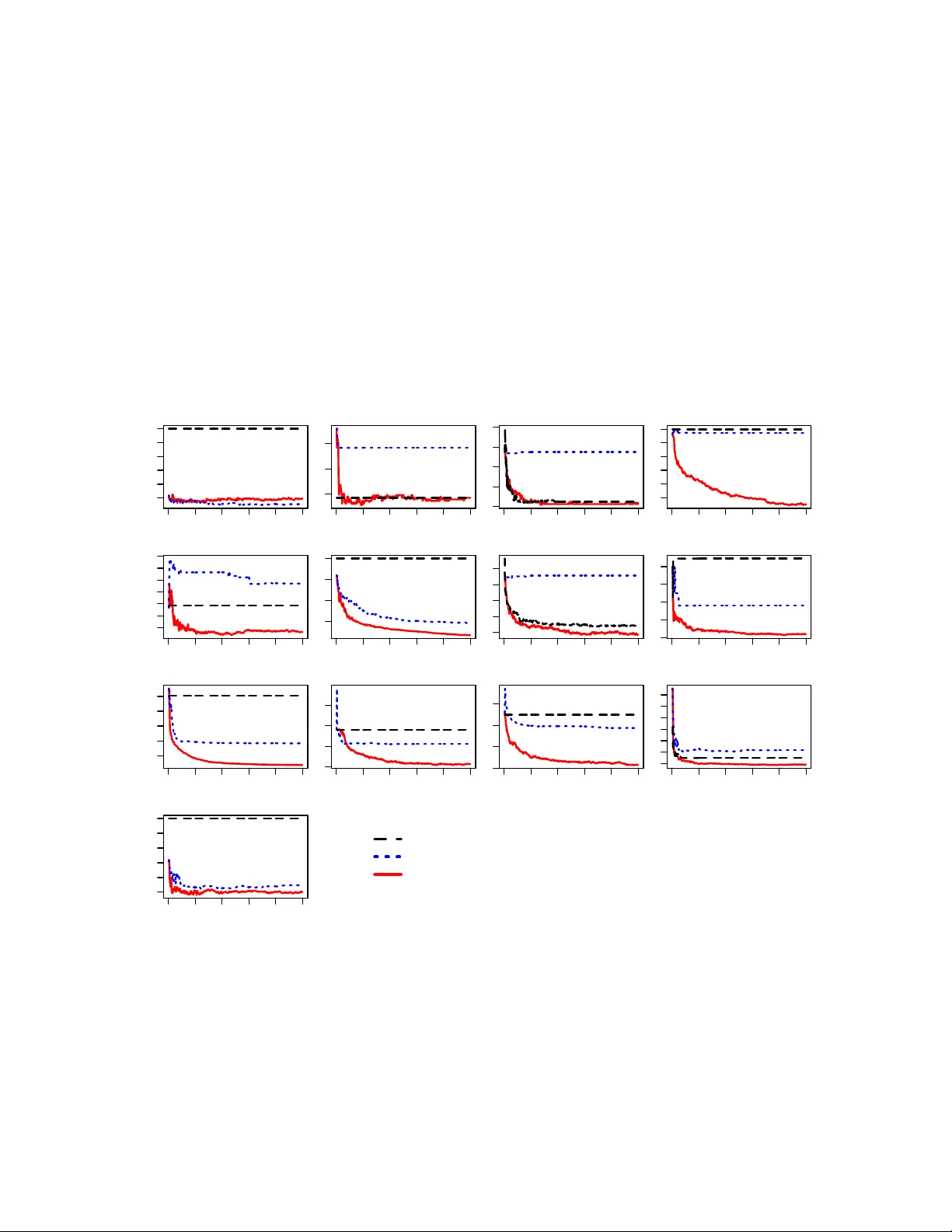
A Theor y of Mul ticlass Boosting A Theory of Multiclass Bo osting Indraneel Mukherjee imukherj@cs.princeton.edu Princ eton University, Dep artment of Computer Scienc e, Princ eton, NJ 08540 USA Rob ert E. Sc hapire schapire@cs.princeton.edu Princ eton University, Dep artment of Computer Scienc e, Princ eton, NJ 08540 USA Editor: Abstract Bo osting com bines w eak classiﬁers to form highly accurate predictors. Although the case of binary classiﬁcation is w ell understoo d, in the m ulticlass setting, the “correct” requiremen ts on the w eak classiﬁer, or the notion of the most eﬃcien t b oosting algorithms are missing. In this pap er, w e create a broad and general framew ork, within which w e mak e precise and iden tify the optimal requirements on the weak-classiﬁer, as well as design the most eﬀectiv e, in a certain sense, b oosting algorithms that assume suc h requiremen ts. Keyw ords: Multiclass, b o osting, weak learning condition, drifting games 1. In tro duction Bo osting (Sc hapire and F reund, 2012) refers to a general tec hnique of com bining rules of th um b, or weak classiﬁers, to form highly accurate combined classiﬁers. Minimal demands are placed on the weak classiﬁers, so that a v ariety of learning algorithms, also called w eak-learners, can be emplo y ed to discov er these simple rules, making the algorithm widely applicable. The theory of bo osting is well-dev eloped for the case of binary classiﬁcation. In particular, the exact requirements on the weak classiﬁers in this setting are known: any algorithm that predicts b etter than random on any distribution ov er the training set is said to satisfy the weak learning assumption. F urther, b o osting algorithms that minimize loss as eﬃciently as p ossible ha ve b een designed. Sp eciﬁcally , it is kno wn that the Bo ost-b y- ma jority (F reund, 1995) algorithm is optimal in a certain s ense, and that AdaBo ost (F reund and Schapire, 1997) is a practical approximation. Suc h an understanding w ould b e desirable in the multiclass setting as well, since man y natural classiﬁcation problems inv olve more than tw o lab els, e.g. recognizing a digit from its image, natural language pro cessing tasks suc h as part-of-sp eec h tagging, and ob ject recognition in vision. Ho w ever, for such m ulticlass problems, a complete theoretical un- derstanding of b oosting is lac king. In particular, w e do not kno w the “correct” wa y to deﬁne the requiremen ts on the w eak classiﬁers, nor has the notion of optimal bo osting b een explored in the multiclass setting. Straigh tforw ard extensions of the binary weak-learning condition to m ulticlass do not w ork. Requiring less error than random guessing on ev ery distribution, as in the binary case, turns out to b e to o w eak for b o osting to b e p ossible when there are more than t wo lab els. On the other hand, requiring more than 50% accuracy ev en when the n um b er of lab els is m uc h larger than tw o is to o stringent, and simple weak classiﬁers like decision stumps fail 1 I. Mukherjee and R. E. Schapire to meet this criterion, even though they often can b e combined to pro duce highly accurate classiﬁers (F reund and Sc hapire, 1996a). The most common approac hes so far hav e relied on reductions to binary classiﬁcation (Allw ein et al., 2000), but it is hardly clear that the w eak-learning conditions implicitly assumed by suc h reductions are the most appropriate. The purp ose of a w eak-learning condition is to clarify the goal of the weak-learner, th us aiding in its design, while providing a sp eciﬁc minimal guaran tee on p erformance that can b e exploited by a b o osting algorithm. These considerations ma y signiﬁcantly impact learning and generalization b ecause knowing the correct w eak-learning conditions migh t allow the use of simpler w eak classiﬁers, whic h in turn can help preven t o verﬁtting. F urthermore, b o osting algorithms that more eﬃciently and eﬀectively minimize training error may prev en t underﬁtting, which can also b e imp ortan t. In this pap er, we create a broad and general framework for studying multiclass bo osting that formalizes the in teraction b etw een the b oosting algorithm and the w eak-learner. Unlike m uc h, but not all, of the previous work on m ulticlass b oosting, w e fo cus sp eciﬁcally on the most natural, and p erhaps weak est, case in which the weak classiﬁers are genuine classiﬁers in the sense of predicting a single multiclass label for each instance. Our new framew ork allo ws us to express a range of w eak-learning conditions, b oth new ones and most of the ones that had previously b een assumed (often only implicitly). Within this formalism, we can also now ﬁnally make precise what is mean t b y c orr e ct weak-learning conditions that are neither to o w eak nor to o strong. W e fo cus particularly on a family of nov el weak-learning conditions that hav e an es- p ecially app ealing form: like the binary conditions, they require p erformance that is only sligh tly b etter than random guessing, though with resp ect to p erformance measures that are more general than ordinary classiﬁcation error. W e in tro duce a whole family of suc h conditions since there are many w a ys of randomly guessing on more than tw o lab els, a k ey diﬀerence b et ween the binary and multiclass settings. Although these conditions imp ose seemingly mild demands on the w eak-learner, we sho w that each one of them is pow erful enough to guaran tee bo ostabilit y , meaning that some com bination of the w eak classiﬁers has high accuracy . And while no individual member of the family is necessary for b o ostabilit y , w e also show that the entire family taken together is necessary in the sense that for every b oostable learning problem, there exists one member of the family that is satisﬁed. Th us, w e ha v e identiﬁed a family of conditions whic h, as a whole, is necessary and suﬃcien t for m ulticlass b oosting. Moreo ver, w e can combine the en tire family into a single w eak-learning condition that is necessary and suﬃcien t b y taking a kind of union, or logical or , of all the mem b ers. This combined condition can also b e expressed in our framew ork. With this understanding, we are able to c haracterize previously studied w eak-learning conditions. In particular, the condition implicitly used by AdaBo ost.MH (Schapire and Singer, 1999), whic h is based on a one-against-all reduction to binary , turns out to be strictly stronger than necessary for b oostability . This also applies to AdaBoost.M1 (F reund and Sc hapire, 1996a), the most direct generalization of AdaBoost to m ulticlass, whose conditions can b e shown to b e equiv alen t to those of AdaBo ost.MH in our setting. On the other hand, the condition implicit to the SAMME algorithm by Zhu et al. (2009) is to o w eak in the sense that ev en when the condition is satisﬁed, no b oosting algorithm can guarantee to driv e down the training error. Finally , the condition implicit to AdaBo ost.MR (Schapire 2 A Theor y of Mul ticlass Boosting and Singer, 1999; F reund and Schapire, 1996a) (also called AdaBoost.M2) turns out to b e exactly necessary and suﬃcient for b o ostabilit y . Emplo ying prop er weak-learning conditions is imp ortan t, but we also need b o osting algorithms that can exploit these conditions to eﬀectively driv e do wn error. F or a giv en w eak-learning condition, the b oosting algorithm that drives do wn training error most eﬃ- cien tly in our framework can be understo o d as the optimal strategy for playing a certain t w o-play er game. These games are non-trivial to analyze. How ever, using the p ow erful ma- c hinery of drifting games (F reund and Opp er, 2002; Sc hapire, 2001), we are able to compute the optimal strategy for the games arising out of eac h weak-learning condition in the family describ ed ab o v e. Compared to earlier work, our optimality results hold more generally and also ac hieve tigh ter b ounds. These optimal strategies ha ve a natural in terpretation in terms of random w alks, a phenomenon that has b een observed in other settings (Ab erneth y et al., 2008; F reund, 1995). W e also analyze the optimal b oosting strategy when using the minimal w eak learning condition, and this p oses additional c hallenges. Firstly , the minimal weak learning condition has m ultiple natural formulations — e.g., as the union of all the conditions in the family describ ed ab o v e, or the formulation used in AdaBo ost.MR — and eac h form ulation leading to a diﬀeren t game sp eciﬁcation. A priori, it is not clear whic h game would lead to the b est strategy . W e resolve this dilemma b y pro ving that the optimal strategies arising out of diﬀerent form ulations of the same w eak learning condition lead to algorithms that are essen tially equally go od, and therefore w e are free to choose whic hever form ulation leads to an easier analysis without fear of suﬀering in p erformance. W e c ho ose the union of conditions form ulation, since it leads to strategies that share the same interpretation in terms of random walks as b efore. Ho w ever, even with this choice, the resulting games are hard to analyze, and although we can explicitly compute the optimum strategies in general, the computational complexity is usually exp onen tial. Nevertheless, w e identify key situations under whic h eﬃcient computation is p ossible. The game-theoretic strategies are non-adaptive in that they presume prior knowledge ab out the e dge , that is, how muc h b etter than random are the w eak classiﬁers. Algorithms that are adaptive, suc h as AdaBo ost, are muc h more practical b ecause they do not require suc h prior information. W e show therefore how to deriv e an adaptiv e b oosting algorithm b y mo difying the game-theoretic strategy based on the minimal condition. This algorithm enjo ys a num b er of theoretical guaran tees. Unlike some of the non-adaptive strategies, it is eﬃcien tly computable, and since it is based on the minimal weak learning condition, it mak es minimal assumptions. In fact, whenev er presen ted with a b o ostable learning problem, this algorithm can approach zero training error at an exponential rate. More imp ortan tly , the algorithm is eﬀective ev en b eyond the b oostability framew ork. In particular, w e show empirical consistency , i.e., the algorithm alwa ys conv erges to the minimum of a certain exp onen tial loss o v er the training data, whether or not the dataset is b o ostable. F urther- more, using the results in (Mukherjee et al., 2011) w e can sho w that this con vergence occurs rapidly . Our fo cus in this pap er is only on minimizing training error, which, for the algorithms w e derive, pro v ably decreases exp onen tially fast with the num b er of rounds of b oosting under b oostability assumptions. Such results can be used in turn to deriv e b ounds on the generalization error using standard techniques that hav e b een applied to other b oosting 3 I. Mukherjee and R. E. Schapire algorithms (Schapire et al., 1998; F reund and Sc hapire, 1997; Koltchinskii and P anchenk o, 2002). Consistency in the multiclass classiﬁcation setting has b een studied by T ew ari and Bartlett (2007) and has b een sho wn to b e tric kier than binary classiﬁcation consistency . Nonetheless, b y following the approac h in (Bartlett and T raskin, 2007) for sho wing con- sistency in the binary setting, we are able to extend the empirical consistency guaran tees to general consistency guaran tees in the multiclass setting: we show that under certain conditions and with suﬃcient data, our adaptive algorithm approaches the Bay es-optim um error on the test dataset. W e presen t exp erimen ts aimed at testing the eﬃcacy of the adaptive algorithm when w orking with a very weak weak-learner to c hec k that the conditions we hav e identiﬁed are indeed weak er than others that had previously been used. W e ﬁnd that our new adaptiv e strategy achiev es low test error compared to other multiclass b oosting algorithms whic h usually hea vily underﬁt. This v alidates the potential practical beneﬁt of a better theoretical understanding of m ulticlass b o osting. Previous work. The ﬁrst b oosting algorithms were given b y Sc hapire (1990) and F re- und (1995), follo wed by their AdaBo ost algorithm (F reund and Schapire, 1997). Multiclass b oosting techniques include AdaBo ost.M1 and AdaBo ost.M2 (F reund and Schapire, 1997), as w ell as AdaBo ost.MH and AdaBo ost.MR (Sc hapire and Singer, 1999). Other approac hes include the w ork by Eibl and Pfeiﬀer (2005); Zh u et al. (2009). There are also more general approac hes that can b e applied to b o osting including (Allw ein et al., 2000; Beygelzimer et al., 2009; Dietteric h and Bakiri, 1995; Hastie and Tibshirani, 1998). Tw o game-theoretic p erspectives ha v e b een applied to b oosting. The ﬁrst one (F reund and Schapire, 1996b; R¨ atsc h and W armuth, 2005) views the w eak-learning condition as a minimax game, while drifting games (Sc hapire, 2001; F reund, 1995) were designed to analyze the most eﬃcient b oosting algorithms. These games hav e b een further analyzed in the multiclass and con tin- uous time setting in (F reund and Opp er, 2002). 2. F ramew ork W e introduce some notation. Unless otherwise stated, matrices will b e denoted by bold capital letters like M , and vectors by bold small letters like v . En tries of a matrix and v ector will be denoted as M ( i, j ) or v ( i ), while M ( i ) will denote the i th row of a matrix. Inner pro duct of tw o vectors u , v is denoted by h u , v i . The F rob enius inner pro duct of t w o matrices T r( MM 0 ) will b e denoted by M • M 0 , where M 0 is the transp ose of M . The indicator function is denoted by 1 [ · ]. The set of all distributions o v er the set { 1 , . . . , k } will b e denoted b y ∆ { 1 , . . . , k } , and in general, the set of all distributions ov er any set S will b e denoted by ∆( S ). In m ulticlass classiﬁcation, w e w an t to predict the lab els of examples lying in some set X . W e are provided a training set of lab eled examples { ( x 1 , y 1 ) , . . . , ( x m , y m ) } , where each example x i ∈ X has a lab el y i in the set { 1 , . . . , k } . Bo osting combines sev eral mildly p o werful predictors, called we ak classiﬁers , to form a highly accurate com bined classiﬁer, and has b een previously applied for m ulticlass clas- siﬁcation. In this paper, we only allo w w eak classiﬁer that predict a single class for eac h example. This is app ealing, since the com bined classiﬁer has the same form, although it 4 A Theor y of Mul ticlass Boosting diﬀers from what has b een used in muc h previous w ork. Later we will expand our framew ork to include multilab el weak classiﬁers, that ma y predict m ultiple lab els p er example. W e adopt a game-theoretic view of b o osting. A game is pla y ed b etw een t wo pla yers, Bo oster and W eak-Learner, for a ﬁxed num b er of rounds T . With binary lab els, Bo oster outputs a distribution in eac h round, and W eak-Learner returns a weak classiﬁer achieving more than 50% accuracy on that distribution. The m ulticlass game is an extension of the binary game. In particular, in each round t : • Bo oster creates a cost-matrix C t ∈ R m × k , sp ecifying to W eak-Learner that the cost of classifying example x i as l is C t ( i, l ). The cost-matrix may not be arbitrary , but should conform to certain restrictions as discussed b elow. • W eak-Learner returns some weak classiﬁer h t : X → { 1 , . . . , k } from a ﬁxed space h t ∈ H so that the cost incurred is C t • 1 h t = m X i =1 C t ( i, h t ( x i )) , is “small enough”, according to some conditions discussed below. Here b y 1 h w e mean the m × k matrix whose ( i, j )-th en try is 1 [ h ( i ) = j ]. • Bo oster computes a w eight α t for the curren t w eak classiﬁer based on ho w m uc h cost w as incurred in this round. A t the end, Bo oster predicts according to the w eigh ted pluralit y vote of the classiﬁers returned in eac h round: H ( x ) M = argmax l ∈{ 1 ,...,k } f T ( x, l ) , where f T ( x, l ) M = T X t =1 1 [ h t ( x ) = l ] α t . (1) By carefully choosing the cost matrices in eac h round, Bo oster aims to minimize the training error of the ﬁnal classifer H , ev en when W eak-Learner is adv ersarial. The restrictions on cost-matrices created by Booster, and the maximum cost W eak-Learner can suﬀer in eac h round, together deﬁne the we ak-le arning c ondition b eing used. F or binary lab els, the traditional w eak-learning condition states: for an y non-negativ e weigh ts w (1) , . . . , w ( m ) on the training set, the error of the weak classﬁer returned is at most (1 / 2 − γ / 2) P i w i . Here γ parametrizes the condition. There are many wa ys to translate this condition into our language. The one with fewest restrictions on the cost-matrices requires lab eling correctly should b e less costly than lab eling incorrectly: ∀ i : C ( i, y i ) ≤ C ( i, ¯ y i ) (here ¯ y i 6 = y i is the other binary lab el), while the restriction on the returned weak classiﬁer h requires less cost than predicting randomly: X i C ( i, h ( x i )) ≤ X i  1 2 − γ 2  C ( i, ¯ y i ) +  1 2 + γ 2  C ( i, y i )  . 5 I. Mukherjee and R. E. Schapire By the corresp ondence w ( i ) = C ( i, ¯ y i ) − C ( i, y i ), w e may verify the tw o conditions are the same. W e will rewrite this condition after making some simplifying assumptions. Henceforth, without loss of generalit y , we assume that the true lab el is alwa ys 1. Let C bin ⊆ R m × 2 consist of matrices C whic h satisfy C ( i, 1) ≤ C ( i, 2). F urther, let U bin γ ∈ R m × 2 b e the matrix whose each row is (1 / 2 + γ / 2 , 1 / 2 − γ / 2). Then, W eak-Learner searching space H satisﬁes the binary w eak-learning condition if: ∀ C ∈ C bin , ∃ h ∈ H : C •  1 h − U bin γ  ≤ 0 . There are t w o main b eneﬁts to this reform ulation. With linear homogeneous constraints, the mathematics is simpliﬁed, as will b e apparen t later. More imp ortan tly , by v arying the restrictions C bin on the cost v ectors and the matrix U bin , we can generate a v ast v ariety of w eak-learning conditions for the multiclass setting k ≥ 2 as w e now sho w. Let C ⊆ R m × k and let B ∈ R m × k b e a matrix whic h we call the b aseline . W e say a weak classiﬁer space H satisﬁes the condition ( C , B ) if ∀ C ∈ C , ∃ h ∈ H : C • ( 1 h − B ) ≤ 0 , i.e., m X i =1 C ( i, h ( i )) ≤ m X i =1 h C ( i ) , B ( i ) i . (2) In (2), the v ariable matrix C sp eciﬁes ho w costly eac h misclassiﬁcation is, while the baseline B sp eciﬁes a w eigh t for eac h misclassiﬁcation. The condition therefore states that a weak classiﬁer should not exceed the a v erage cost when weigh ted according to baseline B . This large class of w eak-learning conditions captures man y previously used conditions, suc h as the ones used by AdaBoost.M1 (F reund and Schapire, 1996a), AdaBo ost.MH (Sc hapire and Singer, 1999) and AdaBo ost.MR (F reund and Sc hapire, 1996a; Schapire and Singer, 1999) (see b elo w), as well as nov el conditions introduced in the next section. By studying this v ast class of weak-learning conditions, we hop e to ﬁnd the one that will serve the main purp ose of the b o osting game: ﬁnding a con v ex combination of w eak classiﬁers that has zero training error. F or this to b e p ossible, at the minim um the w eak classiﬁers should b e suﬃcien tly rich for such a p erfect combination to exist. F or- mally , a collection H of w eak classiﬁers is b o ostable if it is eligible for b o osting in the sense that there exists a distribution λ on this space that linearly separates the data: ∀ i : argmax l ∈{ 1 ,...,k } P h ∈H λ ( h ) 1 [ h ( x i ) = l ] = y i . The weak-learning condition pla ys tw o roles. It rejects spaces that are not b o ostable, and provides an algorithmic means of searc h- ing for the right com bination. Ideally , the second factor will not cause the w eak-learning condition to imp ose additional restrictions on the w eak classiﬁers; in that case, the w eak- learning condition is merely a reform ulation of b eing b o ostable that is more appropriate for deriving an algorithm. In general, it could b e to o str ong , i.e. certain b oostable spaces will fail to satisfy the conditions. Or it could b e to o we ak i.e., non-b o ostable spaces might satisfy such a condition. Bo oster strategies relying on either of these conditions will fail to driv e down error, the former due to underﬁtting, and the latter due to ov erﬁtting. Later w e will describ e conditions captured by our framework that av oid b eing to o weak or too strong. But b efore that, we sho w in the next section ho w our ﬂexible framew ork captures w eak learning conditions that hav e app eared previously in the literature. 6 A Theor y of Mul ticlass Boosting 3. Old conditions In this section, we rewrite, in the language of our framework, the w eak learning condi- tions explicitly or implicitly emplo y ed in the m ulticlass b o osting algorithms SAMME (Zh u et al., 2009), AdaBo ost.M1 (F reund and Sc hapire, 1996a), and AdaBo ost.MH and Ad- aBo ost.MR (Schapire and Singer, 1999). This will b e useful later on for comparing the strengths and weaknesses of the v arious conditions. W e will end this section with a curious equiv alence b etw een the conditions of AdaBo ost.MH and AdaBo ost.M1. Recall that we hav e assumed the correct lab el is 1 for every example. Nev ertheless, w e con tin ue to use y i to denote the correct lab el in this section. 3.1 Old conditions in the new framework Here w e restate, in the language of our new framework, the weak learning conditions of four algorithms that ha ve earlier app eared in the literature. SAMME. The SAMME algorithm (Zh u et al., 2009) requires less error than random guessing on any distribution on the examples. F ormally , a space H satisﬁes the condition if there is a γ 0 > 0 such that, ∀ d (1) , . . . , d ( m ) ≥ 0 , ∃ h ∈ H : m X i =1 d ( i ) 1 [ h ( x i ) 6 = y i ] ≤ (1 − 1 /k − γ 0 ) m X i =1 d ( i ) . (3) Deﬁne a cost matrix C whose entries are given b y C ( i, j ) = ( d ( i ) if j 6 = y i , 0 if j = y i . Then the left hand side of (3) can b e written as m X i =1 C ( i, h ( x i )) = C • 1 h . Next let γ = (1 − 1 /k ) γ 0 and deﬁne baseline U γ to b e the m ulticlass extension of U bin , U γ ( i, l ) = ( (1 − γ ) k + γ if l = y i , (1 − γ ) k if l 6 = y i . Then the righ t hand side of (3) can b e written as m X i =1 X l 6 = y i C ( i, l ) U γ ( i, l ) = C • U γ , since C ( i, y i ) = 0 for every example i . Deﬁne C SAM to b e the follo wing collection of cost matrices: C SAM M = ( C : C ( i, l ) = ( 0 if l = y i , t i if l 6 = y i , for non-negative t 1 , . . . , t m . ) 7 I. Mukherjee and R. E. Schapire Using the last tw o equations, (3) is equiv alent to ∀ C ∈ C SAM , ∃ h ∈ H : C •  1 h − U γ  ≤ 0 . Therefore, the w eak-learning condition of SAMME is giv en by ( C SAM , U γ ). AdaBo ost.M1 Adabo ost.M1 (F reund and Schapire, 1997) measures the p erformance of w eak classiﬁers using ordinary error. It requires 1 / 2 + γ / 2 accuracy with resp ect to any non-negativ e weigh ts d (1) , . . . , d ( m ) on the training set: m X i =1 d ( i ) 1 [ h ( x i ) 6 = y i ] ≤ (1 / 2 − γ / 2) m X i =1 d ( i ) , (4) i.e. m X i =1 d ( i ) J h ( x i ) 6 = y i K ≤ − γ m X i =1 d ( i ) . where J · K is the ± 1 indicator function, taking v alue +1 when its argument is true, and − 1 when false. Using the transformation C ( i, l ) = J l 6 = y i K d ( i ) (5) w e may rewrite (5) as ∀ C ∈ R m × k satisfying 0 ≤ − C ( i, y i ) = C ( i, l ) for l 6 = y i , (6) ∃ h ∈ H : m X i =1 C ( i, h ( x i )) ≤ γ m X i =1 C ( i, y i ) i.e. ∀ C ∈ C M1 , ∃ h ∈ H : C •  1 h − B M1 γ  ≤ 0 , (7) where B M1 γ ( i, l ) = γ 1 [ l = y i ], and C M1 ⊆ R m × k consists of matrices satisfying the con- strain ts in (6). AdaBo ost.MH AdaBoost.MH (Schapire and Singer, 1999) is a popular m ulticlass bo ost- ing algorithm that is based on the one-against-all reduction, and was originally designed to use weak-h yp otheses that return a prediction for ev ery example and ev ery label. The im- plicit w eak learning condition requires that for any matrix with non-negativ e entries d ( i, l ), the weak-h yp othesis should achiev e 1 / 2 + γ accuracy m X i =1    1 [ h ( x i ) 6 = y i ] d ( i, y i ) + X l 6 = y i 1 [ h ( x i ) = l ] d ( i, l )    ≤  1 2 − γ 2  m X i =1 k X l =1 d ( i, l ) . (8) This can b e rewritten as m X i =1    − 1 [ h ( x i ) = y i ] d ( i, y i ) + X l 6 = y i 1 [ h ( x i ) = l ] d ( i, l )    ≤ m X i =1     1 2 − γ 2  X l 6 = y i d ( i, l ) −  1 2 + γ 2  d ( i, y i )    . 8 A Theor y of Mul ticlass Boosting Using the mapping C ( i, l ) = ( d ( i, l ) if l 6 = y i − d ( i, l ) if l = y i , their weak-learning condition may b e rewritten as follows ∀ C ∈ R m × k satisfying C ( i, y i ) ≤ 0 , C ( i, l ) ≥ 0 for l 6 = y i , (9) ∃ h ∈ H : m X i =1 C ( i, h ( x i )) ≤ m X i =1     1 2 + γ 2  C ( i, y i ) +  1 2 − γ 2  X l 6 = y i C ( i, l )    . (10) Deﬁning C MH to b e the space of all cost matrices satisfying the constraints in (9), the ab ov e condition is the same as ∀ C ∈ C MH , ∃ h ∈ H : C •  1 h − B MH γ  ≤ 0 , where B MH γ ( i, l ) = (1 / 2 + γ J l = y i K / 2). AdaBo ost.MR AdaBoost.MR (Sc hapire and Singer, 1999) is based on the all-pairs mul- ticlass to binary reduction. Lik e AdaBo ost.MH, it w as originally designed to use weak- h yp otheses that return a prediction for every example and every lab el. The weak learning condition for AdaBoost.MR requires that for any non-negativ e cost-vectors { d ( i, l ) } l 6 = y i , the w eak-h yp othesis returned should satisfy the following: m X i =1 X l 6 = y i ( 1 [ h ( x i ) = l ] − 1 [ h ( x i ) = y i ]) d ( i, l ) ≤ − γ m X i =1 X l 6 = y i d ( i, l ) i.e. m X i =1    − 1 [ h ( x i ) = y i ] X l 6 = y i d ( i, l ) + X l 6 = y i 1 [ h ( x i ) = l ] d ( i, l )    ≤ − γ m X i =1 X l 6 = y i d ( i, l ) . Substituting C ( i, l ) = ( d ( i, l ) l 6 = y i − P l 6 = y i d ( i, l ) l = y i , w e may rewrite AdaBo ost.MR’s weak-learning condition as ∀ C ∈ R m × k satisfying C ( i, l ) ≥ 0 for l 6 = y i , C ( i, y i ) = − X l 6 = y i C ( i, l ) , (11) ∃ h ∈ H : m X i =1 C ( i, h ( x i )) ≤ − γ 2 m X i =1    − C ( i, y i ) + X l 6 = y i C ( i, l )    . Deﬁning C MR to b e the collection of cost matrices satisfying the constrain ts in (11), the ab o ve condition is the same as ∀ C ∈ C MR , ∃ h ∈ H : C •  1 h − B MR γ  ≤ 0 , where B MR γ ( i, l ) = J l = y i K γ / 2. 9 I. Mukherjee and R. E. Schapire 3.2 A curious equiv alence W e sho w that the w eak learning conditions of AdaBo ost.MH and AdaBoost.M1 are identical in our framework. This is surprising b ecause the original motiv ations b ehind these algo- rithms w ere completely diﬀerent. AdaBoos t.M1 is a direct extension of binary AdaBo ost to the multiclass setting, whereas AdaBo ost.MH is based on the one-against-all multiclass to binary reduction. This equiv alence is a sort of degeneracy , and arises b ecause the w eak classiﬁers b eing used predict single labels per example. With multilabel w eak classiﬁers, for whic h AdaBo ost.MH was originally designed, the equiv alence no longer holds. The pro ofs in this and later sections will mak e use of the follo wing minimax result, that is a w eaker v ersion of Corollary 37.3.2 of (Ro c k afellar, 1970). Theorem 1 (Minimax The or em) L et C, D b e non-empty close d c onvex subsets of R m , R n r esp e ctively, and let K b e a line ar function on C × D . If either C or D is b ounde d, then min v ∈ D max u ∈ C K ( u, v ) = max u ∈ C min v ∈ D K ( u, v ) . Lemma 2 A we ak classiﬁer sp ac e H satisﬁes ( C M1 , B M1 γ ) if and only i f it satisﬁes ( C MH , B MH γ ) . Pro of W e will refer to ( C M1 , B M1 γ ) by M1 and ( C MH , B MH γ ) by MH for brevit y . The pro of is in three steps. Step (i) : If H satisﬁes MH, then it also satisﬁes M1. This follo ws since any constraint (4) imp osed b y M1 on H can b e repro duced by MH b y plugging the following v alues of d ( i, l ) in (8) d ( i, l ) = ( d ( i ) if l = y i 0 if l 6 = y i . Step (ii) : If H satisﬁes M1, then there is a conv ex combination H λ ∗ of the matrices 1 h ∈ H , deﬁned as H λ ∗ M = X h ∈H λ ∗ ( h ) 1 h , suc h that ∀ i :  H λ ∗ − B MH γ  ( i, l ) ( ≥ 0 if l = y i ≤ 0 if l 6 = y i . (12) Indeed, Theorem 1 yields min λ ∈ ∆( H ) max C ∈C M1 C •  H λ − B M1 γ  = max C ∈C M1 min h ∈H C •  1 h − B M1 γ  ≤ 0 , (13) where the inequalit y is a restatement of our assumption that H satisﬁes M1. If λ ∗ is a minimizer of the minmax expression, then H λ ∗ m ust satisfy ∀ i : H λ ∗ ( i, l ) ( ≥ 1 2 + γ 2 if l = y i ≤ 1 2 − γ 2 if l 6 = y i , (14) 10 A Theor y of Mul ticlass Boosting or else some c hoice of C ∈ C M1 can cause C •  H λ ∗ − B M1  to exceed 0. In particular, if H λ ∗ ( i 0 , l ) < 1 / 2 + γ / 2, then  H λ ∗ − B M1 γ  ( i 0 , y i 0 ) < X l 6 = y i 0  H λ ∗ − B M1 γ  ( i 0 , l ) . No w, if we c ho ose C ∈ C M1 as C ( i, l ) =      0 if i 6 = i 0 1 if i = i 0 , l 6 = y i 0 − 1 if i = i 0 , l = y i 0 , then, C •  H λ ∗ − B M1 γ  = −  H λ ∗ − B M1 γ  ( i 0 , y i 0 ) + X l 6 = y i 0  H λ ∗ − B M1 γ  ( i 0 , l ) > 0 , con tradicting the inequalit y in (13). Therefore (14) holds. Eqn. (12), and thus Step (ii), no w follows b y observing that B MH γ , by deﬁnition, satisﬁes ∀ i : B MH γ ( i, l ) = ( 1 2 + γ 2 if l = y i 1 2 − γ 2 if l 6 = y i . Step (iii) If there is some con v ex combination H λ ∗ satisfying (12), then H satisﬁes MH. Recall that B MH consists of entries that are non-p ositiv e on the correct lab els and non-negativ e for incorrect lab els. Therefore, (12) implies 0 ≥ max C ∈C MH C •  H λ ∗ − B MH γ  ≥ min λ ∈ ∆( H ) max C ∈C MH C •  H λ − B MH γ  . On the other hand, using Theorem 1 we hav e min λ ∈ ∆( H ) max C ∈C MH C •  H λ − B MH γ  = max C ∈C MH min h ∈H C •  1 h − B MH γ  . Com bining the tw o, w e get 0 ≥ max C ∈C MH min h ∈H C •  1 h − B MH γ  , whic h is the same as sa ying that H satisﬁes MH’s condition. Steps (ii) and (iii) together imply that if H satisﬁes M1, then it also satisﬁes MH. Along with Step (i), this concludes the pro of. 4. Necessary and suﬃcient weak-learning conditions The binary w eak-learning condition has an app ealing form: for any distribution o ver the examples, the w eak classiﬁer needs to achiev e error not greater than that of a random pla y er who guesses the correct answer with probabilit y 1 / 2 + γ / 2. F urther, this is the w eak est con- dition under whic h b oosting is p ossible as follo ws from a game-theoretic p erspective (F reund and Sc hapire, 1996b; R¨ atsc h and W armuth, 2005) . Multiclass weak-learning conditions with similar prop erties are missing in the literature. In this section w e sho w ho w our framew ork captures such conditions. 11 I. Mukherjee and R. E. Schapire 4.1 Edge-ov er-random conditions In the m ulticlass setting, w e model a random pla y er as a baseline predictor B ∈ R m × k whose ro ws are distributions ov er the lab els, B ( i ) ∈ ∆ { 1 , . . . , k } . The prediction on example i is a sample from B ( i ). W e only consider the space of e dge-over-r andom baselines B eor γ ⊆ R m × k who ha v e a fain t clue ab out the correct answer. More precisely , any baseline B ∈ B eor γ in this space is γ more likely to predict the correct label than an incorrect one on ev ery example i : ∀ l 6 = 1 , B ( i, 1) ≥ B ( i, l ) + γ , with equalit y holding for some l , i.e.: B ( i, 1) = max { B ( i, l ) + γ : l 6 = 1 } . Notice that the edge-o v er-random baselines are diﬀeren t from the baselines used by earlier w eak learning conditions discussed in the previous section. When k = 2, the space B eor γ consists of the unique play er U bin γ , and the binary w eak- learning condition is given b y ( C bin , U bin γ ). The new conditions generalize this to k > 2. In particular, deﬁne C eor to be the m ulticlass extension of C bin : any cost-matrix in C eor should put the least cost on the correct lab el, i.e., the rows of the cost-matrices should come from the set  c ∈ R k : ∀ l, c (1) ≤ c ( l )  . Then, for ev ery baseline B ∈ B eor γ , we in tro duce the condition ( C eor , B ), whic h w e call an e dge-over-r andom w eak-learning condition. Since C • B is the exp ected cost of the edge-ov er-random baseline B on matrix C , the constraints (2) imp osed by the new condition essentially require b etter than random p erformance. Also recall that w e hav e assumed that the true lab el y i of example i in our training set is alwa ys 1. Nevertheless, w e may o ccasionally contin ue to refer to the true lab els as y i . W e no w presen t the central results of this section. The seemingly mild edge-o ver-random conditions guarantee b o ostabilit y , meaning w eak classiﬁers that satisfy an y one such condi- tion can b e com bined to form a highly accurate combined classiﬁer. Theorem 3 (Suﬃciency) If a we ak classiﬁer sp ac e H satisﬁes a we ak-le arning c ondition ( C e or , B ) , for some B ∈ B e or γ , then H is b o ostable. Pro of The pro of is in the spirit of the ones in (F reund and Sc hapire, 1996b). Applying Theorem 1 yields 0 ≥ max C ∈C eor min h ∈H C • ( 1 h − B ) = min λ ∈ ∆( H ) max C ∈C eor C • ( H λ − B ) , where the ﬁrst inequalit y follo ws from the deﬁnition (2) of the w eak-learning condition. Let λ ∗ b e a minimizer of the min-max expression. Unless the ﬁrst entry of each row of ( H λ ∗ − B ) is the largest, the right hand side of the min-max expression can b e made arbitrarily large b y c hoosing C ∈ C eor appropriately . F or example, if in some ro w i , the j th 0 elemen t is strictly larger than the ﬁrst element, b y choosing C ( i, j ) =      − 1 if j = 1 1 if j = j 0 0 otherwise , w e get a matrix in C eor whic h causes C • ( H λ ∗ − B ) to b e equal to C ( i, j 0 ) − C ( i, 1) > 0, an imp ossibilit y by the ﬁrst inequality . 12 A Theor y of Mul ticlass Boosting Therefore, the conv ex combination of the weak classiﬁers, obtained b y choosing each w eak classiﬁer with w eight given b y λ ∗ , p erfectly classiﬁes the training data, in fact with a margin γ . On the other hand, the family of suc h conditions, taken as a whole, is necessary for bo osta- bilit y in the sense that ev ery eligible space of w eak classiﬁers satisﬁes some edge-o ver-random condition. Theorem 4 (Relaxed necessit y) F or every b o ostable we ak classiﬁer sp ac e H , ther e exists a γ > 0 and B ∈ B e or γ such that H satisﬁes the we ak-le arning c ondition ( C e or , B ) . Pro of The pro of shows existence through non-constructive a v eraging arguments. W e will reuse notation from the proof of Theorem 3 ab o ve. H is b o ostable implies there exists some distribution λ ∗ ∈ ∆( H ) such that ∀ j 6 = 1 , i : H λ ∗ ( i, 1) − H λ ∗ ( i, j ) > 0 . Let γ > 0 b e the minimum of the abov e expression ov er all p ossible ( i, j ), and let B = H λ ∗ . Then B ∈ B eor γ , and max C ∈C eor min h ∈H C • ( 1 h − B ) ≤ min λ ∈ ∆( H ) max C ∈C eor C • ( H λ − B ) ≤ max C ∈C eor C • ( H λ ∗ − B ) = 0 , where the equality follows since by deﬁnition H λ ∗ − B = 0 . The max-min expression is at most zero is another wa y of saying that H satisﬁes the w eak-learning condition ( C eor , B ) as in (2). Theorem 4 states that any b oostable w eak classiﬁer space will satisfy some condition in our family , but it do es not help us c ho ose the righ t condition. Exp erimen ts in Section 10 suggest  C eor , U γ  is eﬀective with v ery simple weak-learners compared to p opular bo osting algorithms. (Recall U γ ∈ B eor γ is the edge-ov er-random baseline closest to uniform; it has w eigh t (1 − γ ) /k on incorrect lab els and (1 − γ ) /k + γ on the correct lab el.) Ho wev er, there are theoretical examples showing eac h condition in our family is to o strong. Theorem 5 F or any B ∈ B e or γ , ther e exists a b o ostable sp ac e H that fails to satisfy the c ondition ( C e or , B ) . Pro of W e provide, for any γ > 0 and edge-ov er-random baseline B ∈ B eor γ , a dataset and w eak classiﬁer space that is b oostable but fails to satisfy the condition ( C eor , B ). Pic k γ 0 = γ /k and set m > 1 /γ 0 so that b m (1 / 2 + γ 0 ) c > m/ 2. Our dataset will ha v e m lab eled examples { (0 , y 0 ) , . . . , ( m − 1 , y m − 1 ) } , and m w eak classiﬁers. W e w an t the follo wing symmetries in our weak classiﬁers: • Each w eak classiﬁer correctly classiﬁes b m (1 / 2 + γ 0 ) c examples and misclassiﬁes the rest. • On each example, b m (1 / 2 + γ 0 ) c weak classiﬁers predict correctly . Note the second prop ert y implies b o ostabilit y , since the uniform con v ex combination of all the weak classiﬁers is a p erfect predictor. 13 I. Mukherjee and R. E. Schapire The tw o properties can b e satisﬁed by the follo wing design. A windo w is a con tiguous sequence of examples that may wrap around; for example { i, ( i + 1) mo d m, . . . , ( i + k ) mo d m } is a windo w containing k elemen ts, whic h ma y wrap around if i + k ≥ m . F or eac h windo w of length b m (1 / 2 + γ 0 ) c create a h yp othesis that correctly classiﬁes within the window, and misclassiﬁes outside. This weak-h yp othesis space has size m , and has the required prop erties. W e still ha ve ﬂexibility as to ho w the misclassiﬁcations o ccur, and which cost-matrix to use, which brings us to the next tw o choices: • Whenever a hypothesis misclassiﬁes on example i , it predicts lab el ˆ y i M = argmin { B ( i, l ) : l 6 = y i } . (15) • A cost-matrix is chosen so that the cost of predicting ˆ y i on example i is 1, but for an y other prediction the cost is zero. Observ e this cost-matrix b elongs to C eor . Therefore, ev ery time a w eak classiﬁer predicts incorrectly , it also suﬀers cost 1. Since eac h w eak classiﬁer predicts correctly only within a window of length b m (1 / 2 + γ 0 ) c , it suﬀers cost d m (1 / 2 − γ 0 ) e . On the other hand, by the choice of ˆ y i in (15), B ( i, ˆ y i ) = min { B ( i, 1) − γ , B ( i, 2) , . . . , B ( i, k ) } ≤ 1 k { B ( i, 1) − γ + B ( i, 2) + B ( i, 3) + . . . + B ( i, k ) } = 1 /k − γ /k . So the cost of B on the chosen cost-matrix is at most m (1 /k − γ /k ), which is less than the cost d m (1 / 2 − γ 0 ) e ≥ m (1 / 2 − γ /k ) of any w eak classiﬁer whenev er the num b er of lab els k is more than tw o. Hence our b oostable space of weak classiﬁers fails to satisfy ( C eor , B ). Theorems 4 and 5 can b e interpreted as follows. While a b o ostable space will satisfy some edge-o v er-random condition, without further information about the dataset it is not p ossible to know which particular condition will b e satisﬁed. The kind of prior knowledge required to make this guess correctly is pro vided by Theorem 3: the appropriate w eak learning condition is determined by the distribution of votes on the lab els for each example that a target weak classiﬁer com bination might b e able to get. Even with domain exp ertise, such kno wledge may or may not b e obtainable in practice b efore running b o osting. W e therefore need conditions that assume less. 4.2 The minimal weak learning condition A p erhaps extreme w a y of w eak ening the condition is by requiring the p erformance on a cost matrix to be comp etitive not with a ﬁxe d baseline B ∈ B eor γ , but with the worst of them: ∀ C ∈ C eor , ∃ h ∈ H : C • 1 h ≤ max B ∈B eor γ C • B . (16) 14 A Theor y of Mul ticlass Boosting Condition (16) states that during the course of the same bo osting game, W eak-Learner may c ho ose to beat any edge-ov er-random baseline B ∈ B eor γ , possibly a diﬀerent one for every round and every cost-matrix. This ma y sup erﬁcially seem m uc h to o w eak. On the contrary , this condition turns out to b e equiv alen t to b o ostabilit y . In other words, according to our criterion, it is neither to o weak nor to o strong as a weak-learning condition. How ever, unlik e the edge-ov er-random conditions, it also turns out to b e more diﬃcult to work with algorithmically . F urthermore, this condition can b e shown to b e equiv alen t to the one used by Ad- aBo ost.MR (Schapire and Singer, 1999; F reund and Sc hapire, 1996a). This is perhaps re- mark able since the latter is based on the apparently completely unrelated all-pairs m ulticlass to binary reduction. In Section 3 w e saw that the MR condition is giv en b y ( C MR , B MR γ ), where C MR consists of cost-matrices that put non-negativ e costs on incorrect lab els and whose rows sum up to zero, while B MR γ ∈ R m × k is the matrix that has γ on the ﬁrst column and − γ on all other columns. F urther, the MR condition, and hence (16), can b e sho wn to b e neither to o weak nor to o strong. Theorem 6 (MR) A we ak classiﬁer sp ac e H satisﬁes A daBo ost.MR’s we ak-le arning c on- dition ( C MR , B MR γ ) if and only if it satisﬁes (16) . Mor e over, this c ondition is e quivalent to b eing b o ostable. Pro of W e will sho w the following three conditions are equiv alent: (A) H is b o ostable (B) ∃ γ > 0 such that ∀ C ∈ C eor , ∃ h ∈ H : C • 1 h ≤ max B ∈B eor γ C • B (C) ∃ γ > 0 such that ∀ C ∈ C MR , ∃ h ∈ H : C • 1 h ≤ C • B MR . W e will sho w (A) implies (B), (B) implies (C), and (C) implies (A) to ac hieve the abov e. (A) implies (B) : Immediate from Theorem 2. (B) implies (C) : Supp ose (B) is satisﬁed with 2 γ . W e will show that this implies H satisﬁes ( C MR , B MR γ ). Notice C MR ⊂ C eor . Therefore it suﬃces to show that ∀ C ∈ C MR , B ∈ B eor 2 γ : C •  B − B MR γ  ≤ 0 . Notice that B ∈ B eor 2 γ implies B 0 = B − B MR γ is a matrix whose largest en try in eac h row is in the ﬁrst column of that row. Then, for any C ∈ C MR , C • B 0 can b e written as C • B 0 = m X i =1 k X j =2 C ( i, j )  B 0 ( i, j ) − B 0 ( i, 1)  . Since C ( i, j ) ≥ 0 for j > 1, and B 0 ( i, j ) − B 0 ( i, 1) ≤ 0, we ha v e our result. (C) implies (A) : Applying Theorem 1 0 ≥ max C ∈C MR min h ∈H C •  1 h − B MR γ  = min λ ∈ ∆( H ) max C ∈C MR C •  H λ − B MR γ  . 15 I. Mukherjee and R. E. Schapire h 1 h 2 a 1 2 b 1 2 Figure 1: A weak classiﬁer space which satisﬁes SAMME’s w eak learning condition but is not b oostable. F or an y i 0 and l 0 6 = 1, the follo wing cost-matrix C satisﬁes C ∈ C MR , C ( i, l ) =      0 if i 6 = i 0 or l 6∈ { 1 , l 0 } 1 if i = i 0 , l = l 0 − 1 if i = i 0 , l = 1 . Let λ b elong to the argmin of the min max expression. Then C •  H λ − B MR γ  ≤ 0 implies H λ ( i 0 , 1) − H λ ( i 0 , l 0 ) ≥ 2 γ . Since this is true for all i 0 and l 0 6 = 1, we conclude that the ( C MR , B MR γ ) condition implies b o ostabilit y . This concludes the pro of of equiv alence. Next, w e illustrate the strengths of our minimal w eak-learning condition through concrete comparisons with previous algorithms. Comparison with SAMME. The SAMME algorithm of Zhu et al. (2009) requires the w eak classiﬁers to achiev e less error than uniform random guessing for multiple lab els; in our language, their weak-learning condition is ( C SAM , U γ ), as shown in Section 3, where C SAM consists of cost matrices whose rows are of the form (0 , t, t, . . . ) for some non-negative t . As is w ell-kno wn, this condition is not suﬃcien t for b o osting to b e p ossible. In particular, consider the dataset { ( a, 1) , ( b, 2) } with k = 3 , m = 2, and a w eak classiﬁer space consisting of h 1 , h 2 whic h alw a ys predict 1 , 2, respectively (Figure 1). Since neither classiﬁer distinguishes b et ween a, b w e cannot ac hiev e p erfect accuracy by com bining them in any wa y . Y et, due to the constraints on the cost-matrix, one of h 1 , h 2 will alw a ys manage non-p ositiv e cost while random alw ays suﬀers p ositiv e cost. On the other hand our weak-learning condition allo ws the Bo oster to c ho ose far ric her cost matrices. In particular, when the cost matrix C ∈ C eor is given b y 1 2 3 a − 1 +1 0 b +1 − 1 0, b oth classiﬁers in the ab o ve example suﬀer more loss than the random play er U γ , and fail to satisfy our condition. Comparison with AdaBo ost.MH. AdaBo ost.MH (Schapire and Singer, 1999) was de- signed for use with weak h yp otheses that on eac h example return a prediction for every lab el. When used in our framework, where the weak classiﬁers return only a single mul- ticlass prediction p er example, the implicit demands made b y AdaBo ost.MH on the weak classiﬁer space turn out to b e to o strong. T o demonstrate this, we construct a classiﬁer space that satisﬁes the condition ( C eor , U γ ) in our family , but cannot satisfy AdaBo ost.MH’s 16 A Theor y of Mul ticlass Boosting w eak-learning condition. Note that this do es not imply that the conditions are to o strong when used with more pow erful w eak classiﬁers that return m ultilab el m ulticlass predictions. Consider a space H that has, for ev ery (1 /k + γ ) m element subset of the examples, a classiﬁer that predicts correctly on exactly those elements. The exp ected loss of a randomly c hosen classiﬁer from this space is the same as that of the random pla y er U γ . Hence H satisﬁes this w eak-learning condition. On the other hand, it w as sho wn in Section 3 that AdaBo ost.MH’s weak-learning condition is the pair ( C MH , B MH γ ), where C MH consists of cost matrices with non-negativ e entries on incorrect lab els and non-positive en tries on real lab els, and where eac h ro w of the matrix B MH γ is the v ector (1 / 2 + γ / 2 , 1 / 2 − γ / 2 , . . . , 1 / 2 − γ / 2). A quic k calculation sho ws that for any h ∈ H , and C ∈ C MH with − 1 in the ﬁrst column and zeroes elsewhere, C •  1 h − B MH γ  = 1 / 2 − 1 /k . This is p ositiv e when k > 2, so that H fails to satisfy AdaBo ost.MH’s condition. W e ha v e seen how our framework allo ws us to capture the strengths and weaknesses of old conditions, describ e a whole new family of conditions and also identify the condition making minimal assumptions. In the next few sections, w e show how to design b oosting algorithms that emplo y these new conditions and enjo y strong theoretical guarantees. 5. Algorithms In this section w e devise algorithms by analyzing the b o osting games that employ weak- learning conditions in our framework. W e compute the optim um Bo oster strategy against a completely adv ersarial W eak-Learner, which here is p ermitted to c ho ose w eak classiﬁers without restriction, i.e. the entire space H all of all possible functions mapping examples to lab els. By mo deling W eak-Learner adv ersarially , we mak e absolutely no assumptions on the algorithm it migh t use. Hence, error guarantees enjo y ed in this situation will b e univ ersally applicable. Our algorithms are derived from the very general drifting games framew ork (Schapire, 2001) for solving b o osting games, whic h in turn was inspired by F reund’s Bo ost-b y-ma jority algorithm (F reund, 1995), which we review next. The OS Algorithm. Fix the num b er of rounds T and a weak-learning condition ( C , B ). W e will only consider conditions that are not vacuous , i.e., at least some classiﬁer space satisﬁes the condition, or equiv alently , the space H all satisﬁes ( C , B ). Additionally , we assume the constraints placed by C are on individual rows. In other w ords, there is some subset C 0 ⊆ R k of all possible ro ws, suc h that a cost matrix C b elongs to the collection C if and only if each of its rows b elongs to this subset: C ∈ C ⇐ ⇒ ∀ i : C ( i ) ∈ C 0 . (17) F urther, w e assume C 0 forms a con vex cone i.e c , c 0 ∈ C 0 implies t c + t 0 c 0 ∈ C 0 for any non- negativ e t, t 0 . This also implies that C is a conv ex cone. This is a v ery natural restriction, and is satisﬁed by the space C used by the weak learning conditions of AdaBo ost.MH, AdaBo ost.M1, AdaBo ost.MR, SAMME as well as ev ery edge-o ver-random condition. 1 F or simplicit y of presentation we ﬁx the weigh ts α t = 1 in eac h round. With f T deﬁned 1. All our results hold under the weak er restriction on the space C , where the set of p ossible cost vectors C 0 for a row i could depend on i . F or simplicit y of exp osition, we stick to the more restrictive assumption that C 0 is common across all rows. 17 I. Mukherjee and R. E. Schapire as in (1), whether the ﬁnal h yp otheses output by Bo oster mak es a prediction error on an example i is decided b y whether an incorrect lab el receiv ed the maximum num ber of votes, f T ( i, 1) ≤ max k l =2 f T ( i, l ). Therefore, the optim um Bo oster pay oﬀ can b e written as min C 1 ∈C max h 1 ∈H all : C 1 • ( 1 h 1 − B ) ≤ 0 . . . min C T ∈C max h T ∈H all : C T • ( 1 h T − B ) ≤ 0 1 m m X i =1 L err ( f T ( x i , 1) , . . . , f T ( x i , k )) . (18) where the function L err : R k → R enco des 0-1 error L err ( s ) = 1  s (1) ≤ max l> 1 s ( l )  . (19) In general, w e will also consider other loss functions L : R k → R such as exp onential loss, hinge loss, etc. that upp er-bound error and are pr op er : i.e. L ( s ) is increasing in the w eight of the correct lab el s (1), and decreasing in the weigh ts of the incorrect lab els s ( l ) , l 6 = 1. Directly analyzing the optimal pa y oﬀ is hard. Ho wev er, Sc hapire (2001) observed that the pay oﬀs can b e very well appro ximated b y certain p oten tial functions. Indeed, for an y b ∈ R k deﬁne the p otential function φ b t : R k → R by the following recurrence: φ b 0 = L φ b t ( s ) = min c ∈C 0 max p ∈ ∆ { 1 ,...,k } E l ∼ p  φ b t − 1 ( s + e l )  s.t. E l ∼ p [ c ( l )] ≤ h b , c i , (20) where l ∼ p denotes that label l is sampled from the distribution p , and e l ∈ R k is the unit- v ector whose l th co ordinate is 1 and the remaining co ordinates zero. Notice the recurrence uses the collection of ro ws C 0 instead of the collection of c ost matrices C . When there are T − t rounds remaining (that is, after t rounds of b oosting), these potential functions compute an estimate φ b T − t ( s t ) of whether an example x will be misclassiﬁed, based on its curren t state s t consisting of coun ts of votes receiv ed so far on v arious classes: s t ( l ) = t − 1 X t 0 =1 1 [ h t 0 ( x ) = l ] . (21) Notice this deﬁnition of state assumes that α t = 1 in eac h round. Sometimes, we will choose the w eigh ts diﬀerently . In suc h cases, a more appropriate deﬁnition is the weigh ted state f t ∈ R k , tracking the weigh ted counts of votes receiv ed so far: f t ( l ) = t − 1 X t 0 =1 α t 0 1 [ h t 0 ( x ) = l ] . (22) Ho w ever, unless otherwise noted, w e will assume α t = 1, and so the deﬁnition in (21) will suﬃce. The recurrence in (20) requires the max play er’s response p to satisfy the constrain t that the exp ected cost under the distribution p is at most the inner-pro duct h c , b i . If there is no 18 A Theor y of Mul ticlass Boosting distribution satisfying this requirement, then the v alue of the max expression is −∞ . The existence of a v alid distribution depends on b oth b and c and is captured by the follo wing: ∃ p ∈ ∆ { 1 , . . . , k } : E l ∼ p [ c ( l )] ≤ h c , b i ⇐ ⇒ min l c ( l ) ≤ h b , c i . (23) In this pap er, the v ector b will alwa ys corresp ond to some row B ( i ) of the baseline used in the w eak learning condition. In such a situation, the next lemma sho ws that a distribution satisfying the required constraints will alwa ys exist. Lemma 7 If C 0 is a c one and (17) holds, then for any r ow b = B ( i ) of the b aseline and any c ost ve ctor c ∈ C 0 , (23) holds unless the c ondition ( C , B ) is vacuous. Pro of W e sho w that if (23) does not hold, then the condition is v acuous. Assume that for ro w b = B ( i 0 ) of the baseline, and some choice of cost v ector c ∈ C 0 , (23) does not hold. W e pic k a cost-matrix C ∈ C , such that no weak classiﬁer h can satisfy the requirement (2), implying the condition m ust b e v acuous. The i th 0 ro w of the cost matrix is c , and the remaining rows are 0 . Since C 0 is a cone, 0 ∈ C 0 and hence the cost matrix lies in C . With this choice for C , the condition (2) b ecomes c ( h ( x i )) = C ( i, h ( x i )) ≤ h C ( i ) , B ( i ) i = h c , b i < min l c ( l ) , where the last inequality holds since, by assumption, (23) is not true for this c hoice of c , b . The previous equation is an imp ossibility , and hence no suc h weak classiﬁer h exists, sho wing the condition is v acuous. Lemma 7 shows that the expression in (20) is w ell deﬁned, and tak es on ﬁnite v alues. W e next record an alternate dual form for the same recurrence which will b e useful later. Lemma 8 The r e curr enc e in (20) is e quivalent to φ b t ( s ) = min c ∈C 0 k max l =1 n φ b t − 1 ( s + e l ) − ( c ( l ) − h c , b i ) o . (24) Pro of Using Lagrangean multipliers, we ma y con v ert (20) to an unconstrained expression as follows: φ b t ( s ) = min c ∈C 0 max p ∈ ∆ { 1 ,...,k } min λ ≥ 0 n E l ∼ p h φ b t − 1 ( s + e l ) i − λ ( E l ∼ p [ c ( l )] − h c , b i ) o . Applying Theorem 1 to the inner min-max expression we get φ b t ( s ) = min c ∈C 0 min λ ≥ 0 max p ∈ ∆ { 1 ,...,k } n E l ∼ p h φ b t − 1 ( s + e l ) i − ( E l ∼ p [ λc ( l )] − h λ c , b i ) o . Since C 0 is a cone, c ∈ C 0 implies λ c ∈ C 0 . Therefore w e ma y absorb th e Lagrange m ultiplier in to the cost vector: φ b t ( s ) = min c ∈C 0 max p ∈ ∆ { 1 ,...,k } E l ∼ p h φ b t − 1 ( s + e l ) − ( c ( l ) − h c , b i ) i . F or a ﬁxed c hoice of c , the exp ectation is maximized when the distribution p is concen trated on a single lab el that maximizes the inner expression, which completes our pro of. 19 I. Mukherjee and R. E. Schapire The dual form of the recurrence is useful for optimally choosing the cost matrix in eac h round. When the weak learning condition b eing used is ( C , B ), Schapire (2001) proposed a Bo oster strategy , called the OS strategy , which alwa ys c ho oses the w eigh t α t = 1, and uses the p oten tial functions to construct a cost matrix C t as follo ws. Eac h ro w C t ( i ) of the matrix ac hiev es the minim um of the right hand side of (24) with b replaced by B ( i ), t replaced by T − t , and s replaced by current state s t ( i ): C t ( i ) = argmin c ∈C 0 k max l =1 n φ B ( i ) T − t − 1 ( s + e l ) − ( c ( l ) − h c , B ( i ) i ) o . (25) The follo wing theorem, prov ed in the app endix, pro vides a guarantee for the loss suﬀered b y the OS algorithm, and also shows that it is the game-theoretically optim um strategy when the num b er of examples is large. Similar results hav e b een prov ed by Sc hapire (2001), but our theorem holds muc h more generally , and also achiev es tigh ter low er b ounds. Theorem 9 (Extension of results in (Sc hapire, 2001)) Supp ose the we ak-le arning c on- dition is not vacuous and is given by ( C , B ) , wher e C is such that, for some c onvex c one C 0 ⊆ R k , the c ondition (17) holds. L et the p otential functions φ b t b e deﬁne d as in (20) , and assume the Bo oster employs the OS algorithm, cho osing α t = 1 and C t as in (25) in e ach r ound t . Then the aver age p otential of the states, 1 m m X i =1 φ B ( i ) T − t ( s t ( i )) , never incr e ases in any r ound. In p articular, the loss suﬀer e d after T r ounds of play is at most 1 m m X i =1 φ B ( i ) T ( 0 ) . (26) F urther, under c ertain c onditions, this b ound is ne arly tight. In p articular, assume the loss function do es not vary to o much but satisﬁes sup s , s 0 ∈S T | L ( s ) − L ( s 0 ) | ≤  ( L, T ) , (27) wher e S T , a subset of  s ∈ R k : k s k ∞ ≤ T  , is the set of al l states r e achable in T iter ations, and  ( L, T ) is an upp er b ound on the discr ep ancy of losses b etwe en any two r e achable states when the loss function is L and the total numb er of iter ations is T . Then, for any ε > 0 , when the numb er of examples m is suﬃciently lar ge, m ≥ T  ( L, T ) ε , (28) no Bo oster str ate gy c an guar ante e to achieve in T r ounds a loss that is ε less than the b ound (26) . In order to implemen t the near optimal OS strategy , we need to solve (25). This is compu- tationally only as hard as ev aluating the p oten tials, which in turn reduces to computing the recurrences in (20). In the next few sections, we study how to do this when using v arious losses and w eak learning conditions. 20 A Theor y of Mul ticlass Boosting 6. Solving for any ﬁxed edge-o v er-random condition In this section w e sho w ho w to implement the OS strategy when the weak learning condi- tion is an y ﬁxed edge-o ver-random condition: ( C , B ) for some B ∈ B eor γ . By our previous discussions, this is equiv alent to computing the p oten tial φ b t b y solving the recurrence in (20), where the v ector b corresp onds to some row of the baseline B . Let ∆ k γ ⊆ ∆ { 1 , . . . , k } denote the set of all edge-o v er-random distributions on { 1 , . . . , k } with γ more w eigh t on the ﬁrst co ordinate: ∆ k γ = { b ∈ ∆ { 1 , . . . , k } : b (1) − γ = max { b (2) , . . . , b ( k ) }} . (29) Note, that B eor γ consists of all matrices whose rows b elong to the set ∆ k γ . Therefore we are in terested in computing φ b , where b is an arbitrary edge-o ver-random distribution: b ∈ ∆ k γ . W e b egin b y simplifying the recurrence (20) satisﬁed by such p oten tials, and show how to compute the optimal cost matrix in terms of the p oten tials. Lemma 10 Assume L is pr op er, and b ∈ ∆ k γ is an e dge-over-r andom distribution. Then the r e curr enc e (20) may b e simpliﬁe d as φ b t ( s ) = E l ∼ b [ φ t − 1 ( s + e l )] . (30) F urther, if the c ost matrix C t is chosen as fol lows C t ( i, l ) = φ b T − t − 1 ( s t ( i ) + e l ) , (31) then C t satisﬁes the c ondition in (25) , and henc e is the optimal choic e. Pro of Let C eor 0 ⊆ R k denote all v ectors c satisfying ∀ l : c (1) ≤ c ( l ). Then, w e hav e φ b t ( s ) = min c ∈C eor 0 max p ∈ ∆ { 1 ,...,k } E l ∼ p [ φ t − 1 ( s + e l )] s.t. E l ∼ p [ c ( l )] ≤ E l ∼ b [ c ( l )] , ( by (20) ) = min c ∈C eor 0 max p ∈ ∆ min λ ≥ 0 n E l ∼ p h φ b t − 1 ( s + e l ) i + λ ( E l ∼ b [ c ( l )] − E l ∼ p [ c ( l )]) o (Lagrangean) = min c ∈C eor 0 min λ ≥ 0 max p ∈ ∆ E l ∼ p h φ b t − 1 ( s + e l ) i + λ h b − p , c i (Theorem 1) = min c ∈C eor 0 max p ∈ ∆ E l ∼ p h φ b t − 1 ( s + e l ) i + h b − p , c i (absorb λ into c ) = max p ∈ ∆ min c ∈C eor 0 E l ∼ p h φ b t − 1 ( s + e l ) i + h b − p , c i (Theorem 1) . Unless b (1) − p (1) ≤ 0 and b ( l ) − p ( l ) ≥ 0 for eac h l > 1, the quantit y h b − p , c i can b e made arbitrarily small for appropriate c hoices of c ∈ C eor 0 . The max-play er is therefore forced to constrain its c hoices of p , and the ab o ve expression b ecomes max p ∈ ∆ E l ∼ p  φ b t − 1 ( s + e l )  s . t . b ( l ) − q ( l ) ( ≥ 0 if l = 1 , ≤ 0 if l > 1 . 21 I. Mukherjee and R. E. Schapire Lemma 6 of (Sc hapire, 2001) states that if L is pr op er (as deﬁned here), so is φ b t ; the same result can b e extended to our drifting games. This implies the optimal c hoice of p in the ab o ve expression is in fact the distribution that puts as small w eight as p ossible in the ﬁrst co ordinate, namely b . Therefore the optimum choice of p is b , and the p oten tial is the same as in (30). W e end the pro of b y sho wing that the choice of cost matrix in (31) is optimum. Theo- rem 9 states that a cost matrix C t is the optimum c hoice if it satisﬁes (25), that is, if the expression k max l =1 n φ B ( i ) T − t − 1 ( s + e l ) − ( C t ( i, l ) − h C t ( i ) , B ( i ) i ) o (32) is equal to min c ∈C 0 k max l =1 n φ B ( i ) T − t − 1 ( s + e l ) − ( c ( l ) − h c , B ( i ) i ) o = φ B ( i ) T − t ( s ) , (33) where the equalit y in (33) follows from (24). If C t ( i ) is c hosen as in (31), then, for any lab el l , the expression within max in (32) ev aluates to φ B ( i ) T − t − 1 ( s + e l ) −  φ B ( i ) T − t − 1 ( s + e l ) − h C t ( i ) , B ( i ) i  = h B ( i ) , C t ( i ) i = E l ∼ B ( i ) [ C t ( i, l )] = E l ∼ B ( i ) h φ B ( i ) T − t − 1 ( s + e l ) i = φ B ( i ) T − t ( s ) , where the last equality follo ws from (30). Therefore the max expression in (32) is also equal to φ B ( i ) T − t ( s ), which is what w e needed to sho w. Eq. (31) in Lemma 10 implies the cost matrix chosen b y the OS strategy can b e expressed in terms of the p oten tials, whic h is the only thing left to calculate. F ortunately , the simpli- ﬁcation (30) of the drifting games recurrence, allows the p otentials to b e solv ed completely in terms of a random-walk R t b ( x ). This random v ariable denotes the p osition of a particle after t time steps, that starts at lo cation x ∈ R k , and in eac h step mov es in direction e l with probability b ( l ). Corollary 11 The r e curr enc e in (30) c an b e solve d as fol lows: φ b t ( s ) = E  L  R t b ( s )  . (34) Pro of Inductively assuming φ b t − 1 ( x ) = E  L ( R t − 1 b ( x ))  , φ t ( s ) = E l ∼ b  L ( R t − 1 b ( s ) + e l )  = E  L ( R t b ( s ))  . The last equalit y follo ws by observing that the random p osition R t − 1 b ( s ) + e l is distributed as R t b ( s ) when l is sampled from b . Lemma 10 and Corollary 11 together imply: Theorem 12 Assume L is pr op er and b ∈ ∆ k γ is an e dge-over-r andom distribution. Then the p otential φ b t , deﬁne d by the r e curr enc e in (20) , has the solution given in (34) in terms of r andom walks. 22 A Theor y of Mul ticlass Boosting Before we can compute (34), w e need to choose a loss function L . W e next consider t wo options for the loss — the non-conv ex 0-1 error, and exp onential loss. Exp onen tial Loss. The exp onential loss serv es as a smo oth conv ex proxy for discon- tin uous non-conv ex 0-1 error (19) that we would ultimately lik e to b ound, and is given b y L exp η ( s ) = k X l =2 e η ( s l − s 1 ) . (35) The parameter η can b e thought of as the w eigh t in each round, that is, α t = η in each round. Then notice that the w eigh ted state f t of the examples, deﬁned in (22), is related to the un weigh ted states s t as f t ( l ) = η s t ( l ). Therefore the exponential loss function in (35) directly measures the loss of the weigh ted state as L exp ( f t ) = k X l =2 e f t ( l ) − f t (1) . (36) Because of this corresp ondence, the optimal strategy with the loss function L exp and α t = η is the same as that using loss L exp η and α t = 1. W e study the latter setting so that we ma y use the results derived earlier. With the choice of the exp onen tial loss L exp η , the p oten tials are easily computed, and in fact hav e a closed form solution. Theorem 13 If L exp η is as in (35) , wher e η is non-ne gative, then the solution in The or em 12 evaluates to φ b t ( s ) = P k l =2 ( a l ) t e η l ( s l − s 1 ) , wher e a l = 1 − ( b 1 + b l ) + e η b l + e − η b 1 . The pro of by induction is straigh tforward. By tuning the weigh t η , eac h a l can b e alwa ys made less than 1. This ensures the exp onential loss decays exp onen tially with rounds. In particular, when B = U γ (so that the condition is ( C eor , U γ )), the relev ant p oten tial φ t ( s ) or φ t ( f ) is given b y φ t ( s ) = φ t ( f ) = κ ( γ , η ) t k X l =2 e η ( s l − s 1 ) = κ ( γ , η ) t k X l =2 e f l − f 1 (37) where κ ( γ , η ) = 1 + (1 − γ ) k  e η + e − η − 2  −  1 − e − η  γ . (38) The cost-matrix output by the OS algorithm can be simpliﬁed b y rescaling, or adding the same num b er to each co ordinate of a cost v ector, without aﬀecting the constrain ts it imposes on a w eak classiﬁer, to the following form C ( i, l ) = ( ( e η − 1) e η ( s l − s 1 ) if l > 1 , ( e − η − 1) P k l =2 e η ( s l − s 1 ) if l = 1 . Using the corresp ondence b et ween unw eighted and weigh ted states, the ab o v e may also b e rewritten as: C ( i, l ) = ( ( e η − 1) e f l − f 1 if l > 1 , ( e − η − 1) P k l =2 e f l − f 1 if l = 1 . (39) 23 I. Mukherjee and R. E. Schapire With suc h a choice, Theorem 9 and the form of the p oten tial guaran tee that the a v erage loss 1 m m X i =1 L exp η ( s t ( i )) = 1 m m X i =1 L exp ( f t ( i )) (40) of the states c hanges b y a factor of at most κ ( γ , η ) every round. Therefore the ﬁnal loss, whic h upper b ounds the error, i.e., the fraction of misclassiﬁed training examples, is at most ( k − 1) κ ( γ , η ) T . Since this upp er bound holds for an y v alue of η , we ma y tune it to optimize the b ound. Setting η = ln (1 + γ ), the error can b e upp er b ounded b y ( k − 1) e − T γ 2 / 2 . Zero-one Loss. There is no simple closed form solution for the p oten tial when using the zero-one loss L err (19). How ever, we may compute the p oten tials eﬃcien tly as follo ws. T o compute φ b t ( s ), w e need to ﬁ nd the probabilit y that a random w alk (making steps according to b ) of length t in Z k , starting at s will end up in a region where the loss function is 1. Any suc h random walk will consist of x l steps in direction e l where the non-negativ e P l x l = t . The probabilit y of eac h such path is Q l b x l l . F urther, there are exactly  t x 1 ,...,x k  suc h paths. Starting at state s , such a path will lead to a correct answ er only if s 1 + x 1 > s l + x l for eac h l > 1. Hence we ma y write the p oten tial φ b t ( s ) as φ b t ( s ) = 1 − t X x 1 ,...,x k  t x 1 ,...,x k  Q k l =1 b x l l s.t. x 1 + . . . + x k = t ∀ l : x l ≥ 0 ∀ l : x l + s l ≤ x 1 + s 1 . Since the x l ’s are restricted to b e integers, this problem is presumably hard. In particular, the only algorithms known to the authors that tak e time logarithmic in t is also exp onen tial in k . How ev er, b y using dynamic programming, we can compute the summation in time p olynomial in | s l | , t and k . In fact, the run time is alwa ys O ( t 3 k ), and at least Ω( tk ). The b ounds on error we achiev e, although not in closed form, are muc h tighter than those obtainable using exp onen tial loss. The exp onential loss analysis yields an error upp er b ound of ( k − 1) e − T γ 2 / 2 . Using a diﬀerent initial distribution, Sc hapire and Singer (1999) ac hiev e the sligh tly better b ound p ( k − 1) e − T γ 2 / 2 . How ev er, when the edge γ is small and the num ber of rounds are few, eac h b ound is greater than 1 and hence trivial. On the other hand, the bounds computed b y the abov e dynamic program are sensible for all v alues of k , γ and T . When b is the γ -biased uniform distribution b = ( 1 − γ k + γ , 1 − γ k , 1 − γ k , . . . , 1 − γ k ) a table con taining the error upper b ound φ b T (0) for k = 6, γ = 0 and small v alues for the num ber of rounds T is shown in Figure 2(a); note that with the exp onen tial loss, the b ound is alw a ys 1 if the edge γ is 0. F urther, the bounds due to the exponential loss analyses seem to imply that the dep endence of the error on the num ber of lab els is monotonic. How ever, a plot of the tighter b ounds with edge γ = 0 . 1, n um b er of rounds T = 10 against v arious v alues of k , sho wn in Figure 2(b), indicates that the true dep endence is more complicated. Therefore the tigh ter analysis also pro vides qualitativ e insights not obtainable via the exp onen tial loss b ound. 24 A Theor y of Mul ticlass Boosting T φ b T ( 0 ) T φ b T ( 0 ) 0 1.00 6 0.90 1 0.83 7 0.91 2 0.97 8 0.90 3 0.93 9 0.89 4 0.89 10 0.89 5 0.89 (a) 0 50 100 150 200 0.50 0.55 0.60 0.65 0.70 0.75 0.80 T = 10, edge = 0.1 k phi(0) (b) Figure 2: Plot of p oten tial v alue φ b T ( 0 ) where b is the γ -biased uniform distribution: b = ( 1 − γ k + γ , 1 − γ k , 1 − γ k , . . . , 1 − γ k ). (a): Poten tial v alues (rounded to tw o decimal places) for diﬀeren t n um b er of rounds T using γ = 0 and k = 6. These are b ounds on the error, and less than 1 even when the edge and n umber of rounds are small. (b): Poten tial v alues for diﬀerent num b er of classes k , with γ = 0 . 1, and T = 10. These are tight estimates for the optimal error, and y et not monotonic in the n umber of classes. 7. Solving for the minimal weak learning condition In the previous section we saw ho w to ﬁnd the optimal b oosting strategy when using an y ﬁxed edge-o v er-random c ondition. How ev er as we hav e seen b efore, these conditions can b e stronger than necessary , and therefore lead to b o osting algorithms that require addi- tional assumptions. Here w e show how to compute the optimal algorithm while using the w eak est weak learning condition, provided b y (16), or equiv alen tly the condition used by AdaBo ost.MR, ( C MR , B MR γ ). Since there are t wo p ossible form ulations for the minimal con- dition, it is not immediately clear which to use to compute the optimal b o osting strategy . T o resolv e this, w e ﬁrst show that the optimal b o osting strategy based on any form ulation of a necessary and suﬃcient weak learning condition is the same. Ha ving resolved this am- biguit y , w e show how to compute this strategy for the exp onen tial loss and 0-1 error using the ﬁrst form ulation. 7.1 Game-theoretic equiv alence of necessary and suﬃcien t w eak-learning conditions In this section w e study the eﬀect of the w eak learning condition on the game-theoretically optimal b oosting strategy . W e introduce the notion of game-the or etic e quivalenc e b et w een t w o weak learning conditions, that determines if the pay oﬀs (18) of the optimal b o osting strategies based on the t w o conditions are iden tical. This is diﬀerent from the usual notion of equiv alence b et w een t wo conditions, which holds if an y w eak classiﬁer space satisﬁes b oth conditions or neither condition. In fact we pro v e that game-theoretic equiv alence is a 25 I. Mukherjee and R. E. Schapire broader notion; in other words, equiv alence implies game-theoretic equiv alence. A sp ecial case of this general result is that any tw o weak learning conditions that are necessary and suﬃcient, and hence equiv alen t to b o ostabilit y , are also game-theoretically equiv alent. In particular, so are the conditions of AdaBo ost.MR and (16), and the resulting optimal Bo oster strategies enjoy equally go o d pay oﬀs. W e conclude that in order to derive the optimal b o osting strategy that uses the minimal weak-learning condition, it is sound to use either of these tw o formulations. The purp ose of a w eak learning condition ( C , B ) is to imp ose restrictions on the W eak- Learner’s resp onses in each round. These restrictions are captured b y subsets of the weak classiﬁer space as follows. If Bo oster chooses cost-matrix C ∈ C in a round, the W eak- Learner’s resp onse h is restricted to the subset S C ⊆ H all deﬁned as S C = n h ∈ H all : C • 1 h ≤ C • B o . Th us, a weak learning condition is essentially a family of subsets of the w eak classiﬁer space. F urther, smaller subsets mean fewer options for W eak-Learner, and hence b etter pa y oﬀs for the optimal b o osting strategy . Based on this idea, w e may deﬁne when a weak learning condition ( C 1 , B 1 ) is game-the or etic al ly str onger than another condition ( C 2 , B 2 ) if the following holds: F or every subset S C 2 in the second condition (that is C 2 ∈ C 2 ), there is a subset S C 1 in the ﬁrst condition (that is C 1 ∈ C 1 ), such that S C 1 ⊆ S C 2 . Mathematically , this may b e written as follows: ∀ C 1 ∈ C 1 , ∃ C 2 ∈ C 2 : S C 1 ⊆ S C 2 . In tuitiv ely , a game theoretically stronger condition will allo w Bo oster to place similar or stricter restrictions on W eak-Learner in eac h round. Therefore, the optimal Bo oster pay oﬀ using a game-theoretically stronger condition is at least equally go o d, if not b etter. It therefore follows that if tw o conditions are b oth game-theoretically stronger than eac h other, the corresp onding Booster pay oﬀs must be equal, that is they m ust be game-the or etic al ly e quivalent . Note that game-theoretic equiv alence of tw o conditions do es not mean that they are iden tical as families of subsets, for we ma y arbitrarily add large and “useless” subsets to the tw o conditions without aﬀecting the Booster pa y oﬀs, since these subsets will never b e used b y an optimal Bo oster strategy . In fact w e next show that game-theoretic equiv alence is a broader notion than just equiv alence. Theorem 14 Supp ose ( C 1 , B 1 ) and ( C 2 , B 2 ) ar e two e quivalent we ak le arning c onditions, that is, every sp ac e H satisﬁes b oth or neither c ondition. Then e ach c ondition is game- the or etic al ly str onger than the other, and henc e game-the or etic al ly e quivalent. Pro of W e argue by contradiction. Assume that despite equiv alence, the ﬁrst condition (without loss of generality) includes a particularly hard subset S C 1 ⊆ H all , C 1 ∈ C 1 whic h is not smaller than any subset in the second condition. In particular, for every subset S C 2 , C 2 ∈ C 2 in the second condition is satisﬁed b y some weak classiﬁer h C 2 not satisfying the hard subset in the ﬁrst condition: h C 2 ∈ S C 2 \ S C 1 . Therefore, the space H = { h C 2 : C 2 ∈ C 2 } , 26 A Theor y of Mul ticlass Boosting formed by just these classiﬁers satisﬁes the second condition, but has an empty in tersection with S C 1 . In other w ords, H satisﬁes the second but not the ﬁrst condition, a contradiction to their equiv alence. An immediate corollary is the game theoretic equiv alence of necessary and equiv alen t con- ditions. Corollary 15 Any two ne c essary and suﬃcient we ak le arning c onditions ar e game-the or etic al ly e quivalent. In p articular the optimum Bo oster str ate gies b ase d on A daBo ost.MR’s c ondition ( C MR , B MR γ ) and (16) have e qual p ayoﬀs. Therefore, in deriving the optimal Bo oster strategy , it is sound to work with either Ad- aBo ost.MR’s condition or (16). In the next section, we actually compute the optimal strategy using the latter formulation. 7.2 Optimal strategy with the minimal conditions In this section w e compute the optimal Bo oster strategy that uses the minim um w eak learning condition pro vided in (16). W e c ho ose this instead of AdaBo ost.MR’s condition b ecause this description is more closely related to the edge-ov er-random conditions, and the resulting algorithm has a close relationship to the ones derived for ﬁxed edge-ov er- random conditions, and therefore more insightful. How ever, this form ulation do es not state the condition as a single pair ( C , B ), and therefore w e cannot directly use the result of Theorem 9. Instead, we deﬁne new p oten tials and a mo diﬁed OS strategy that is still nearly optimal, and this constitutes the ﬁrst part of this section. In the second part, w e sho w how to compute these new p oten tials and the resulting OS strategy . 7.2.1 Modified potentials and OS stra tegy The condition in (16) is not stated as a single pair ( C eor , B ), but uses all p ossible edge- o v er-random baselines B ∈ B eor γ . Therefore, w e mo dify the deﬁnitions (20) of the potentials accordingly to extract an optimal Bo oster strategy . Recall that ∆ k γ is deﬁned in (29) as the set of all edge-o v er-random distributions which constitute the ro ws of edge-ov er-random baselines B ∈ B eor γ . Using these, deﬁne new p oten tials φ t ( s ) as follo ws: φ t ( s ) = min c ∈C eor 0 max b ∈ ∆ k γ max p ∈ ∆ { 1 ,...,k } E l ∼ p [ φ t − 1 ( s + e l )] s.t. E l ∼ p [ c ( l )] ≤ h b , c i . (41) The main diﬀerence betw een (41) and (20) is that while the older p otentials w ere deﬁned using a ﬁxed v ector b corresp onding to some row in the ﬁxed baseline B , the new deﬁnition tak es the maximum o v er all p ossible rows b ∈ ∆ k γ that an edge-ov er-random baseline B ∈ B eor γ ma y hav e. As b efore, we ma y write the recurrence in (41) in its dual form φ t ( s ) = min c ∈C eor 0 max b ∈ ∆ k γ k max l =1 { φ t − 1 ( s + e l ) − ( c ( l ) − h c , b i ) } . (42) The pro of is very similar to that of Lemma 8 and is omitted. W e may now deﬁne a new OS strategy that c ho oses a cos t-matrix in round t analogously: C t ( i ) ∈ argmin c ∈C eor 0 max b ∈ ∆ k γ k max l =1 { φ t − 1 ( s + e l ) − ( c ( l ) − h c , b i ) } . (43) 27 I. Mukherjee and R. E. Schapire where recall that s t ( i ) denotes the state vector (deﬁned in (21)) of example i . With this strategy , w e can sho w an optimality result very similar to Theorem 9. Theorem 16 Supp ose the we ak-le arning c ondition is given by (16) . L et the p otential func- tions φ b t b e deﬁne d as in (41) , and assume the Bo oster employs the mo diﬁe d OS str ate gy, cho osing α t = 1 and C t as in (43) in e ach r ound t . Then the aver age p otential of the states, 1 m m X i =1 φ T − t ( s t ( i )) , never incr e ases in any r ound. In p articular, the loss suﬀer e d after T r ounds of play is at most φ T ( 0 ) . F urther, for any ε > 0 , when the loss function satisﬁes (27) and the numb er of examples m is as lar ge as in (28) , no Bo oster str ate gy c an guar ante e to achieve less than φ T ( 0 ) − ε loss in T r ounds. The pro of is v ery similar to that of Theorem 9 and is omitted. 7.2.2 Computing the new potentials. Here w e show how to compute the new p oten tials. The resulting algorithms will require exp onen tial time, and we pro vide some empirical evidence sho wing that this might b e necessary . Finally , we show ho w to carry out the computations eﬃcien tly in certain sp ecial situations. An exp onen tial time algorithm. Here we show how the p oten tials may b e computed as the exp ected loss of some random walk, just as w e did for the potentials arising with ﬁxed edge-o v er-random conditions. The m ain diﬀerence is there will b e several random w alks to c ho ose from. W e ﬁrst b egin b y simplifying the recurrence (41), and expressing the optimal cost matrix in (43) in terms of the p oten tials, just as w e did in Lemma 10 for the case of ﬁxed edge- o v er-random conditions. Lemma 17 Assume L is pr op er. Then the r e curr enc e (41) may b e simpliﬁe d as φ t ( s ) = max b ∈ ∆ k γ E l ∼ b [ φ t − 1 ( s + e l )] . (44) F urther, if the c ost matrix C t is chosen as fol lows: C t ( i, l ) = φ T − t − 1 ( s t ( i ) + e l ) , (45) then C t satisﬁes the c ondition in (43) . The pro of is v ery similar to that of Lemma 10 and is omitted. Eq. (45) implies that, as b efore, computing the optimal Bo oster strategy reduces to computing the new p oten tials. One computational diﬃculty created b y the new deﬁnitions (41) or (44) is that they require inﬁnitely man y p ossible distributions b ∈ ∆ k γ to b e considered. W e show that we may in fact restrict our attention to only ﬁnitely many of such distributions describ ed next. 28 A Theor y of Mul ticlass Boosting A t any state s and n um b er of remaining iterations t , let π b e a p erm utation of the co ordinates { 2 , . . . , k } that sorts the p otential v alues: φ t − 1  s + e π ( k )  ≥ φ t − 1  s + e π ( k − 1)  ≥ . . . ≥ φ t − 1  s + e π (2)  . (46) F or an y p ermutation π of the co ordinates { 2 , . . . , k } , let b π a denote the γ -biased uniform distribution on the a co ordinates { 1 , π k , π k − 1 , . . . , π k − a +2 } : b π a ( l ) =      1 − γ a + γ if l = 1 1 − γ a if l ∈ { π k , . . . , π k − a +2 } 0 otherwise. (47) Then, the next lemma sho ws that w e may restrict our attention to only the distributions { b π 2 , . . . , b π k } when ev aluating the recurrence in (44). Lemma 18 Fix a state s and r emaining r ounds of b o osting t . L et π b e a p ermutation of the c o or dinates { 2 , . . . , k } satisfying (46) , and deﬁne b π a as in (47) . Then the r e curr enc e (44) may b e simpliﬁe d as fol lows: φ t ( s ) = max b ∈ ∆ k γ E l ∼ b [ φ t − 1 ( s + e l )] = max 2 ≤ a ≤ k E l ∼ b π a [ φ t − 1 ( s + e l )] . (48) Pro of Assume (by relab eling the co ordinates if necessary) that π is the iden tit y p erm u- tation, that is, π (2) = 2 , . . . , π ( k ) = k . Observe that the righ t hand side of (44) is at least as muc h the righ t hand side of (48) since the former considers more distributions. W e complete the pro of b y showing that the former is also at most the latter. By (44), we ma y assume that some optimal b satisﬁes b ( k ) = · · · = b ( k − a + 2) = b (1) − γ , b ( k − a + 1) ≤ b (1) − γ , b ( k − a ) = · · · = b (2) = 0 . Therefore, b is a distribution supp orted on a + 1 elements, with the minim um w eigh t placed on element k − a + 1. This implies b ( k − a + 1) ∈ [0 , 1 / ( a + 1)]. No w, E l ∼ b [ φ t − 1 ( s + e l )] may b e written as γ · φ t − 1 ( s + e 1 ) + b ( k − a + 1) φ t − 1 ( s + e k − a +1 ) + (1 − γ − b ( k − a + 1)) φ t − 1 ( s + e 1 ) + φ t − 1 ( s + e k − a +2 ) + . . . φ t − 1 ( s + e k ) a = γ · φ t − 1 ( s + e 1 ) + b ( k − a + 1) 1 − γ φ t − 1 ( s + e k − a +1 ) + (1 − γ ) n  1 − b ( k − a + 1) 1 − γ  φ t − 1 ( s + e 1 ) + φ t − 1 ( s + e k − a +2 ) + . . . φ t − 1 ( s + e k ) a o Replacing b ( k − a + 1) b y x in the ab o v e expression, we get a linear function of x . When restricted to [0 , 1 / ( a + 1)] the maxim um v alue is attained at a b oundary p oin t. F or x = 0, the expression b ecomes γ · φ t − 1 ( s + e 1 ) + (1 − γ ) φ t − 1 ( s + e 1 ) + φ t − 1 ( s + e k − a +2 ) + . . . φ t − 1 ( s + e k ) a . 29 I. Mukherjee and R. E. Schapire F or x = 1 / ( a + 1), the expression b ecomes γ · φ t − 1 ( s + e 1 ) + (1 − γ ) φ t − 1 ( s + e 1 ) + φ t − 1 ( s + e k − a +1 ) + . . . φ t − 1 ( s + e k ) a + 1 . Since b ( k − a + 1) lies in [0 , 1 / ( a + 1)], the optimal v alue is at most the maximum of the t w o. Ho w ever eac h of these last t wo expressions is at most the right hand side of (48), completing the pro of. Unra v eling (48), w e ﬁnd that φ t ( s ) is the exp ected loss of the ﬁnal state reac hed by some random walk of t steps starting at state s . How ev er, the num b er of p ossibilities for the random-w alk is huge; indeed, the distribution at eac h step can b e an y of the k − 1 p ossibilities b π a for a ∈ { 2 , . . . , k } , where the parameter a denotes the size of the supp ort of the γ - biased uniform distribution chosen at eac h step. In other w ords, at a giv en state s with t rounds of b o osting remaining, the parameter a determines the num b er of directions the optimal random walk will consider taking; we will therefore refer to a as the de gr e e of the random walk giv en ( s , t ). Now, the total n um b er of states reac hable in T steps is O  T k − 1  . If the degree assignmen t ev ery such state, for every v alue of t ≤ T is ﬁxed in adv ance, a = { a ( s , t ) : t ≤ T , s reachable } , we may identify a unique random walk R a ,t ( s ) of length t starting at step s . Therefore the p oten tial may be computed as φ t ( s ) = max a E  R a ,t ( s )  . (49) A dynamic programming approac h for computing (49) requires time and memory linear in the n umber of diﬀeren t states reach able b y a random w alk that takes T co ordinate steps: O ( T k − 1 ). This is exp onen tial in the dataset size, and hence impractical. In the next tw o sections w e show that p erhaps there may not b e any wa y of com puting these eﬃciently in general, but pro vide eﬃcient algorithms in certain sp ecial cases. Hardness of ev aluating the p oten tials. Here w e pro vide empirical evidence for the hardness of computing the new potentials. W e ﬁrst identify a computationally easier prob- lem, and show that even that is probably hard to compute. Eq. (48) implies that if the p oten tials were eﬃciently computable, the correct v alue of the degree a could b e determined eﬃcien tly . The problem of determining the degree a given the state s and remaining rounds t is therefore easier than ev aluating the p oten tials. How ever, a plot of the degrees against states and remaining rounds, henceforth called a de gr e e map , rev eals very little structure that might b e captured by a computationally eﬃcient function. W e include three suc h degree maps in Figure 3. Only three classes k = 3 are used, and the loss function is 0-1 error. W e also ﬁx the n um b er T of remaining rounds of b o osting and the v alue of the edge γ for eac h plot. F or ease of presen tation, the 3-dimensional states s = ( s 1 , s 2 , s 3 ) are compressed in to 2-dimensional pixel co ordinates ( u = s 2 − s 1 , v = s 3 − s 2 ). It can b e sho wn that this do es not tak e a wa y information required to ev aluate the potentials or the degree at an y pixel ( u, v ). F urther, only those states are considered whose compressed co ordinates u, v lie in the range [ − T , T ]; in T rounds, these account for all the reachable states. The degrees are indicated on the plot by colors. Our discussion in the previous sections implies that the possible v alues of the degree is 2 or 3. When the degree at a pixel ( u, v ) is 3, the pixel is colored green, and when the degre e is 2, it is colored black. 30 A Theor y of Mul ticlass Boosting − 20 − 10 0 10 20 − 20 − 10 0 10 20 T = 20 ● ● ● ● ● ● ● ● ● ● ● ● ● ● ● ● ● ● ● ● ● ● ● ● ● ● ● ● ● ● ● ● ● ● ● ● ● ● ● ● ● ● ● ● ● ● ● ● ● ● ● ● ● ● ● ● ● ● ● ● ● ● ● ● ● ● ● ● ● ● ● ● ● ● ● ● ● ● ● ● ● ● ● ● ● ● ● ● ● ● ● ● ● ● ● ● ● ● ● ● ● ● ● ● ● ● ● ● ● ● ● ● ● ● ● ● ● ● ● ● ● ● ● ● ● ● ● ● ● ● ● ● ● ● ● ● ● ● ● ● ● ● ● ● ● ● ● ● ● ● ● ● ● ● ● ● ● ● ● ● ● ● ● ● ● ● ● ● ● ● ● ● ● ● ● ● ● ● ● ● ● ● ● ● ● ● ● ● ● ● ● ● ● ● ● ● ● ● ● ● ● ● ● ● ● ● ● ● ● ● ● ● ● ● ● ● ● ● ● ● ● ● ● ● ● ● ● ● ● ● ● ● ● ● ● ● ● ● ● ● ● ● ● ● ● ● ● ● ● ● ● ● ● ● ● ● ● ● ● ● ● ● ● ● ● ● ● ● ● ● ● ● ● ● ● ● ● ● ● ● ● ● ● ● ● ● ● ● ● ● ● ● ● ● ● ● ● ● ● ● ● ● ● ● ● ● ● ● ● ● ● ● ● ● ● ● ● ● ● ● ● ● ● ● ● ● ● ● ● ● ● ● ● ● ● ● ● ● ● ● ● ● ● ● ● ● ● ● ● ● ● ● ● ● ● ● ● ● ● ● ● ● ● ● ● ● ● ● ● ● ● ● ● ● ● ● ● ● ● ● ● ● ● ● ● ● ● ● ● ● ● ● ● ● ● ● ● ● ● ● ● ● ● ● ● ● ● ● ● ● ● ● ● ● ● ● ● ● ● ● ● ● ● ● ● ● ● ● ● ● ● ● ● ● ● ● ● ● ● ● ● ● ● ● ● ● ● ● ● ● ● ● ● ● ● ● ● ● ● ● ● ● ● ● ● ● ● ● ● ● ● ● ● ● ● ● ● ● ● ● ● ● ● ● ● ● ● ● ● ● ● ● ● ● ● ● ● ● ● ● ● ● ● ● ● ● ● ● ● ● ● ● ● ● ● ● ● ● ● ● ● ● ● ● ● ● ● ● ● ● ● ● ● ● ● ● ● ● ● ● ● ● ● ● ● ● ● ● ● ● ● ● ● ● ● ● ● ● ● ● ● ● ● ● ● ● ● ● ● ● ● ● ● ● ● ● ● ● ● ● ● ● ● ● ● ● ● ● ● ● ● ● ● ● ● ● ● ● ● ● ● ● ● ● ● ● ● ● ● ● ● ● ● ● ● ● ● ● ● ● ● ● ● ● ● ● ● ● ● ● ● ● ● ● ● ● ● ● ● ● ● ● ● ● ● ● ● ● ● ● ● ● ● ● ● ● ● ● ● ● ● ● ● ● ● ● ● ● ● ● ● ● ● ● ● ● ● ● ● ● ● ● ● ● ● ● ● ● ● ● ● ● ● ● ● ● ● ● ● ● ● ● ● ● ● ● ● ● ● ● ● ● ● ● ● ● ● ● ● ● ● ● ● ● ● ● ● ● ● ● ● ● ● ● ● ● ● ● ● ● ● ● ● ● ● ● ● ● ● ● ● ● ● ● ● ● ● ● ● ● ● ● ● ● ● ● ● ● ● ● ● ● ● ● ● ● ● ● ● ● ● ● ● ● ● ● ● ● ● ● ● ● ● ● ● ● ● ● ● ● ● ● ● ● ● ● ● ● ● ● ● ● ● ● ● ● ● ● ● ● ● ● ● ● ● ● ● ● ● ● ● ● ● ● ● ● ● ● ● ● ● ● ● ● ● ● ● ● ● ● ● ● ● ● ● ● ● ● ● ● ● ● ● ● ● ● ● ● ● ● ● ● ● ● ● ● ● ● ● ● ● ● ● ● ● ● ● ● ● ● ● ● ● ● ● ● ● ● ● ● ● ● ● ● ● ● ● ● ● ● ● ● ● ● ● ● ● ● ● ● ● ● ● ● ● ● ● ● ● ● ● ● ● ● ● ● ● ● ● ● ● ● ● ● ● ● ● ● ● ● ● ● ● ● ● ● ● ● ● ● ● ● ● ● ● ● ● ● ● ● ● ● ● ● ● ● ● ● ● ● ● ● ● ● ● ● ● ● ● ● ● ● ● ● ● ● ● ● ● ● ● ● ● ● ● ● ● ● ● ● ● ● ● ● ● ● ● ● ● ● ● ● ● ● ● ● ● ● ● ● ● ● ● ● ● ● ● ● ● ● ● ● ● ● ● ● ● ● ● ● ● ● ● ● ● ● ● ● ● ● ● ● ● ● ● ● ● ● ● ● ● ● ● ● ● ● ● ● ● ● ● ● ● ● ● ● ● ● ● ● ● ● ● ● ● ● ● ● ● ● ● ● ● ● ● ● ● ● ● ● ● ● ● ● ● ● ● ● ● ● ● ● ● ● ● ● ● ● ● ● ● ● ● ● ● ● ● ● ● ● ● ● ● ● ● ● ● ● ● ● ● ● ● ● ● ● ● ● ● ● ● ● ● ● ● ● ● ● ● ● ● ● ● ● ● ● ● ● ● ● ● ● ● ● ● ● ● ● ● ● ● ● ● ● ● ● ● ● ● ● ● ● ● ● ● ● ● ● ● ● ● ● ● ● ● ● ● ● ● ● ● ● ● ● ● ● ● ● ● ● ● ● ● ● ● ● ● ● ● ● ● ● ● ● ● ● ● ● ● ● ● ● ● ● ● ● ● ● ● ● ● ● ● ● ● ● ● ● ● ● ● ● ● ● ● ● ● ● ● ● ● ● ● ● ● ● ● ● ● ● ● ● ● ● ● ● ● ● ● ● ● ● ● ● ● ● ● ● ● ● ● ● ● ● ● ● ● ● ● ● ● ● ● ● ● ● ● ● ● ● ● ● ● ● ● ● ● ● ● ● ● ● ● ● ● ● ● ● ● ● ● ● ● ● ● ● ● ● ● ● ● ● ● ● ● ● ● ● ● ● ● ● ● ● ● ● ● ● ● ● ● ● ● ● ● ● ● ● ● ● ● ● ● ● ● ● ● ● ● ● ● ● ● ● ● ● ● ● ● ● ● ● ● ● ● ● ● ● ● ● ● ● ● ● ● ● ● ● ● ● ● ● ● ● ● ● ● ● ● ● ● ● ● ● ● ● ● ● ● ● ● ● ● ● ● ● ● ● ● ● ● ● ● ● ● ● ● ● ● ● ● ● ● ● ● ● ● ● ● ● ● ● ● ● ● ● ● ● ● ● ● ● ● ● ● ● ● ● ● ● ● ● ● ● ● ● ● ● ● ● ● ● ● ● ● ● ● ● ● ● ● ● ● ● ● ● ● ● ● ● ● ● ● ● ● ● ● ● ● ● ● ● ● ● ● ● ● ● ● ● ● ● ● ● ● ● ● ● ● ● ● ● ● ● ● ● ● ● ● ● ● ● ● ● ● ● ● ● ● ● ● ● ● ● ● ● ● ● ● ● ● ● ● ● ● ● ● ● ● ● ● ● ● ● ● ● ● ● ● ● ● ● ● ● ● ● ● ● ● ● ● ● ● ● ● ● ● ● ● ● ● ● ● ● ● ● ● ● ● ● ● ● ● ● ● ● ● ● ● ● ● ● ● ● ● ● ● ● ● ● ● ● ● ● ● ● ● ● ● ● ● ● ● ● ● ● ● ● ● ● ● ● ● ● ● ● ● ● ● ● ● ● ● ● ● ● ● ● ● ● ● ● ● ● ● ● ● ● ● ● ● ● ● ● ● ● ● ● ● ● ● ● ● ● ● ● ● ● ● ● ● ● ● ● ● ● ● ● ● ● ● ● ● ● ● ● ● ● ● ● ● ● ● ● ● ● ● ● ● ● ● ● ● ● ● ● ● ● ● ● ● ● ● ● ● ● ● ● ● ● ● ● ● ● ● ● ● ● ● ● ● ● ● ● ● ● ● ● ● ● ● ● ● ● ● ● ● ● ● ● ● ● ● ● ● ● ● ● ● ● ● ● ● ● ● ● ● ● ● ● ● ● ● ● ● ● ● ● ● − 40 − 20 0 20 40 − 40 − 20 0 20 40 T = 50 ● ● ● ● ● ● ● ● ● ● ● ● ● ● ● ● ● ● ● ● ● ● ● ● ● ● ● ● ● ● ● ● ● ● ● ● ● ● ● ● ● ● ● ● ● ● ● ● ● ● ● ● ● ● ● ● ● ● ● ● ● ● ● ● ● ● ● ● ● ● ● ● ● ● ● ● ● ● ● ● ● ● ● ● ● ● ● ● ● ● ● ● ● ● ● ● ● ● ● ● ● ● ● ● ● ● ● ● ● ● ● ● ● ● ● ● ● ● ● ● ● ● ● ● ● ● ● ● ● ● ● ● ● ● ● ● ● ● ● ● ● ● ● ● ● ● ● ● ● ● ● ● ● ● ● ● ● ● ● ● ● ● ● ● ● ● ● ● ● ● ● ● ● ● ● ● ● ● ● ● ● ● ● ● ● ● ● ● ● ● ● ● ● ● ● ● ● ● ● ● ● ● ● ● ● ● ● ● ● ● ● ● ● ● ● ● ● ● ● ● ● ● ● ● ● ● ● ● ● ● ● ● ● ● ● ● ● ● ● ● ● ● ● ● ● ● ● ● ● ● ● ● ● ● ● ● ● ● ● ● ● ● ● ● ● ● ● ● ● ● ● ● ● ● ● ● ● ● ● ● ● ● ● ● ● ● ● ● ● ● ● ● ● ● ● ● ● ● ● ● ● ● ● ● ● ● ● ● ● ● ● ● ● ● ● ● ● ● ● ● ● ● ● ● ● ● ● ● ● ● ● ● ● ● ● ● ● ● ● ● ● ● ● ● ● ● ● ● ● ● ● ● ● ● ● ● ● ● ● ● ● ● ● ● ● ● ● ● ● ● ● ● ● ● ● ● ● ● ● ● ● ● ● ● ● ● ● ● ● ● ● ● ● ● ● ● ● ● ● ● ● ● ● ● ● ● ● ● ● ● ● ● ● ● ● ● ● ● ● ● ● ● ● ● ● ● ● ● ● ● ● ● ● ● ● ● ● ● ● ● ● ● ● ● ● ● ● ● ● ● ● ● ● ● ● ● ● ● ● ● ● ● ● ● ● ● ● ● ● ● ● ● ● ● ● ● ● ● ● ● ● ● ● ● ● ● ● ● ● ● ● ● ● ● ● ● ● ● ● ● ● ● ● ● ● ● ● ● ● ● ● ● ● ● ● ● ● ● ● ● ● ● ● ● ● ● ● ● ● ● ● ● ● ● ● ● ● ● ● ● ● ● ● ● ● ● ● ● ● ● ● ● ● ● ● ● ● ● ● ● ● ● ● ● ● ● ● ● ● ● ● ● ● ● ● ● ● ● ● ● ● ● ● ● ● ● ● ● ● ● ● ● ● ● ● ● ● ● ● ● ● ● ● ● ● ● ● ● ● ● ● ● ● ● ● ● ● ● ● ● ● ● ● ● ● ● ● ● ● ● ● ● ● ● ● ● ● ● ● ● ● ● ● ● ● ● ● ● ● ● ● ● ● ● ● ● ● ● ● ● ● ● ● ● ● ● ● ● ● ● ● ● ● ● ● ● ● ● ● ● ● ● ● ● ● ● ● ● ● ● ● ● ● ● ● ● ● ● ● ● ● ● ● ● ● ● ● ● ● ● ● ● ● ● ● ● ● ● ● ● ● ● ● ● ● ● ● ● ● ● ● ● ● ● ● ● ● ● ● ● ● ● ● ● ● ● ● ● ● ● ● ● ● ● ● ● ● ● ● ● ● ● ● ● ● ● ● ● ● ● ● ● ● ● ● ● ● ● ● ● ● ● ● ● ● ● ● ● ● ● ● ● ● ● ● ● ● ● ● ● ● ● ● ● ● ● ● ● ● ● ● ● ● ● ● ● ● ● ● ● ● ● ● ● ● ● ● ● ● ● ● ● ● ● ● ● ● ● ● ● ● ● ● ● ● ● ● ● ● ● ● ● ● ● ● ● ● ● ● ● ● ● ● ● ● ● ● ● ● ● ● ● ● ● ● ● ● ● ● ● ● ● ● ● ● ● ● ● ● ● ● ● ● ● ● ● ● ● ● ● ● ● ● ● ● ● ● ● ● ● ● ● ● ● ● ● ● ● ● ● ● ● ● ● ● ● ● ● ● ● ● ● ● ● ● ● ● ● ● ● ● ● ● ● ● ● ● ● ● ● ● ● ● ● ● ● ● ● ● ● ● ● ● ● ● ● ● ● ● ● ● ● ● ● ● ● ● ● ● ● ● ● ● ● ● ● ● ● ● ● ● ● ● ● ● ● ● ● ● ● ● ● ● ● ● ● ● ● ● ● ● ● ● ● ● ● ● ● ● ● ● ● ● ● ● ● ● ● ● ● ● ● ● ● ● ● ● ● ● ● ● ● ● ● ● ● ● ● ● ● ● ● ● ● ● ● ● ● ● ● ● ● ● ● ● ● ● ● ● ● ● ● ● ● ● ● ● ● ● ● ● ● ● ● ● ● ● ● ● ● ● ● ● ● ● ● ● ● ● ● ● ● ● ● ● ● ● ● ● ● ● ● ● ● ● ● ● ● ● ● ● ● ● ● ● ● ● ● ● ● ● ● ● ● ● ● ● ● ● ● ● ● ● ● ● ● ● ● ● ● ● ● ● ● ● ● ● ● ● ● ● ● ● ● ● ● ● ● ● ● ● ● ● ● ● ● ● ● ● ● ● ● ● ● ● ● ● ● ● ● ● ● ● ● ● ● ● ● ● ● ● ● ● ● ● ● ● ● ● ● ● ● ● ● ● ● ● ● ● ● ● ● ● ● ● ● ● ● ● ● ● ● ● ● ● ● ● ● ● ● ● ● ● ● ● ● ● ● ● ● ● ● ● ● ● ● ● ● ● ● ● ● ● ● ● ● ● ● ● ● ● ● ● ● ● ● ● ● ● ● ● ● ● ● ● ● ● ● ● ● ● ● ● ● ● ● ● ● ● ● ● ● ● ● ● ● ● ● ● ● ● ● ● ● ● ● ● ● ● ● ● ● ● ● ● ● ● ● ● ● ● ● ● ● ● ● ● ● ● ● ● ● ● ● ● ● ● ● ● ● ● ● ● ● ● ● ● ● ● ● ● ● ● ● ● ● ● ● ● ● ● ● ● ● ● ● ● ● ● ● ● ● ● ● ● ● ● ● ● ● ● ● ● ● ● ● ● ● ● ● ● ● ● ● ● ● ● ● ● ● ● ● ● ● ● ● ● ● ● ● ● ● ● ● ● ● ● ● ● ● ● ● ● ● ● ● ● ● ● ● ● ● ● ● ● ● ● ● ● ● ● ● ● ● ● ● ● ● ● ● ● ● ● ● ● ● ● ● ● ● ● ● ● ● ● ● ● ● ● ● ● ● ● ● ● ● ● ● ● ● ● ● ● ● ● ● ● ● ● ● ● ● ● ● ● ● ● ● ● ● ● ● ● ● ● ● ● ● ● ● ● ● ● ● ● ● ● ● ● ● ● ● ● ● ● ● ● ● ● ● ● ● ● ● ● ● ● ● ● ● ● ● ● ● ● ● ● ● ● ● ● ● ● ● ● ● ● ● ● ● ● ● ● ● ● ● ● ● ● ● ● ● ● ● ● ● ● ● ● ● ● ● ● ● ● ● ● ● ● ● ● ● ● ● ● ● ● ● ● ● ● ● ● ● ● ● ● ● ● ● ● ● ● ● ● ● ● ● ● ● ● ● ● ● ● ● ● ● ● ● ● ● ● ● ● ● ● ● ● ● ● ● ● ● ● ● ● ● ● ● ● ● ● ● ● ● ● ● ● ● ● ● ● ● ● ● ● ● ● ● ● ● ● ● ● ● ● ● ● ● ● ● ● ● ● ● ● ● ● ● ● ● ● ● ● ● ● ● ● ● ● ● ● ● ● ● ● ● ● ● ● ● ● ● ● ● ● ● ● ● ● ● ● ● ● ● ● ● ● ● ● ● ● ● ● ● ● ● ● ● ● ● ● ● ● ● ● ● ● ● ● ● ● ● ● ● ● ● ● ● ● ● ● ● ● ● ● ● ● ● ● ● ● ● ● ● ● ● ● ● ● ● ● ● ● ● ● ● ● ● ● ● ● ● ● ● ● ● ● ● ● ● ● ● ● ● ● ● ● ● ● ● ● ● ● ● ● ● ● ● ● ● ● ● ● ● ● ● ● ● ● ● ● ● ● ● ● ● ● ● ● ● ● ● ● ● ● ● ● ● ● ● ● ● ● ● ● ● ● ● ● ● ● ● ● ● ● ● ● ● ● ● ● ● ● ● ● ● ● ● ● ● ● ● ● ● ● ● ● ● ● ● ● ● ● ● ● ● ● ● ● ● ● ● ● ● ● ● ● ● ● ● ● ● ● ● ● ● ● ● ● ● ● ● ● ● ● ● ● ● ● ● ● ● ● ● ● ● ● ● ● ● ● ● ● ● ● ● ● ● ● ● ● ● ● ● ● ● ● ● ● ● ● ● ● ● ● ● ● ● ● ● ● ● ● ● ● ● ● ● ● ● ● ● ● ● ● ● ● ● ● ● ● ● ● ● ● ● ● ● ● ● ● ● ● ● ● ● ● ● ● ● ● ● ● ● ● ● ● ● ● ● ● ● ● ● ● ● ● ● ● ● ● ● ● ● ● ● ● ● ● ● ● ● ● ● ● ● ● ● ● ● ● ● ● ● ● ● ● ● ● ● ● ● ● ● ● ● ● ● ● ● ● ● ● ● ● ● ● ● ● ● ● ● ● ● ● ● ● ● ● ● ● ● ● ● ● ● ● ● ● ● ● ● ● ● ● ● ● ● ● ● ● ● ● ● ● ● ● ● ● ● ● ● ● ● ● ● ● ● ● ● ● ● ● ● ● ● ● ● ● ● ● ● ● ● ● ● ● ● ● ● ● ● ● ● ● ● ● ● ● ● ● ● ● ● ● ● ● ● ● ● ● ● ● ● ● ● ● ● ● ● ● ● ● ● ● ● ● ● ● ● ● ● ● ● ● ● ● ● ● ● ● ● ● ● ● ● ● ● ● ● ● ● ● ● ● ● ● ● ● ● ● ● ● ● ● ● ● ● ● ● ● ● ● ● ● ● ● ● ● ● ● ● ● ● ● ● ● ● ● ● ● ● ● ● ● ● ● ● ● ● ● ● ● ● ● ● ● ● ● ● ● ● ● ● ● ● ● ● ● ● ● ● ● ● ● ● ● ● ● ● ● ● ● ● ● ● ● ● ● ● ● ● ● ● ● ● ● ● ● ● ● ● ● ● ● ● ● ● ● ● ● ● ● ● ● ● ● ● ● ● ● ● ● ● ● ● ● ● ● ● ● ● ● ● ● ● ● ● ● ● ● ● ● ● ● ● ● ● ● ● ● ● ● ● ● ● ● ● ● ● ● ● ● ● ● ● ● ● ● ● ● ● ● ● ● ● ● ● ● ● ● ● ● ● ● ● ● ● ● ● ● ● ● ● ● ● ● ● ● ● ● ● ● ● ● ● ● ● ● ● ● ● ● ● ● ● ● ● ● ● ● ● ● ● ● ● ● ● ● ● ● ● ● ● ● ● ● ● ● ● ● ● ● ● ● ● ● ● ● ● ● ● ● ● ● ● ● ● ● ● ● ● ● ● ● ● ● ● ● ● ● ● ● ● ● ● ● ● ● ● ● ● ● ● ● ● ● ● ● ● ● ● ● ● ● ● ● ● ● ● ● ● ● ● ● ● ● ● ● ● ● ● ● ● ● ● ● ● ● ● ● ● ● ● ● ● ● ● ● ● ● ● ● ● ● ● ● ● ● ● ● ● ● ● ● ● ● ● ● ● ● ● ● ● ● ● ● ● ● ● ● ● ● ● ● ● ● ● ● ● ● ● ● ● ● ● ● ● ● ● ● ● ● ● ● ● ● ● ● ● ● ● ● ● ● ● ● ● ● ● ● ● ● ● ● ● ● ● ● ● ● ● ● ● ● ● ● ● ● ● ● ● ● ● ● ● ● ● ● ● ● ● ● ● ● ● ● ● ● ● ● ● ● ● ● ● ● ● ● ● ● ● ● ● ● ● ● ● ● ● ● ● ● ● ● ● ● ● ● ● ● ● ● ● ● ● ● ● ● ● ● ● ● ● ● ● ● ● ● ● ● ● ● ● ● ● ● ● ● ● ● ● ● ● ● ● ● ● ● ● ● ● ● ● ● ● ● ● ● ● ● ● ● ● ● ● ● ● ● ● ● ● ● ● ● ● ● ● ● ● ● ● ● ● ● ● ● ● ● ● ● ● ● ● ● ● ● ● ● ● ● ● ● ● ● ● ● ● ● ● ● ● ● ● ● ● ● ● ● ● ● ● ● ● ● ● ● ● ● ● ● ● ● ● ● ● ● ● ● ● ● ● ● ● ● ● ● ● ● ● ● ● ● ● ● ● ● ● ● ● ● ● ● ● ● ● ● ● ● ● ● ● ● ● ● ● ● ● ● ● ● ● ● ● ● ● ● ● ● ● ● ● ● ● ● ● ● ● ● ● ● ● ● ● ● ● ● ● ● ● ● ● ● ● ● ● ● ● ● ● ● ● ● ● ● ● ● ● ● ● ● ● ● ● ● ● ● ● ● ● ● ● ● ● ● ● ● ● ● ● ● ● ● ● ● ● ● ● ● ● ● ● ● ● ● ● ● ● ● ● ● ● ● ● ● ● ● ● ● ● ● ● ● ● ● ● ● ● ● ● ● ● ● ● ● ● ● ● ● ● ● ● ● ● ● ● ● ● ● ● ● ● ● ● ● ● ● ● ● ● ● ● ● ● ● ● ● ● ● ● ● ● ● ● ● ● ● ● ● ● ● ● ● ● ● ● ● ● ● ● ● ● ● ● ● ● ● ● ● ● ● ● ● ● ● ● ● ● ● ● ● ● ● ● ● ● ● ● ● ● ● ● ● ● ● ● ● ● ● ● ● ● ● ● ● ● ● ● ● ● ● ● ● ● ● ● ● ● ● ● ● ● ● ● ● ● ● ● ● ● ● ● ● ● ● ● ● ● ● ● ● ● ● ● ● ● ● ● ● ● ● ● ● ● ● ● ● ● ● ● ● ● ● ● ● ● ● ● ● ● ● ● ● ● ● ● ● ● ● ● ● ● ● ● ● ● ● ● ● ● ● ● ● ● ● ● ● ● ● ● ● ● ● ● ● ● ● ● ● ● ● ● ● ● ● ● ● ● ● ● ● ● ● ● ● ● ● ● ● ● ● ● ● ● ● ● ● ● ● ● ● ● ● ● ● ● ● ● ● ● ● ● ● ● ● ● ● ● ● ● ● ● ● ● ● ● ● ● ● ● ● ● ● ● ● ● ● ● ● ● ● ● ● ● ● ● ● ● ● ● ● ● ● ● ● ● ● ● ● ● ● ● ● ● ● ● ● ● ● ● ● ● ● ● ● ● ● ● ● ● ● ● ● ● ● ● ● ● ● ● ● ● ● ● ● ● ● ● ● ● ● ● ● ● ● ● ● ● ● ● ● ● ● ● ● ● ● ● ● ● ● ● ● ● ● ● ● ● ● ● ● ● ● ● ● ● ● ● ● ● ● ● ● ● ● ● ● ● ● ● ● ● ● ● ● ● ● ● ● ● ● ● ● ● ● ● ● ● ● ● ● ● ● ● ● ● ● ● ● ● ● ● ● ● ● ● ● ● ● ● ● ● ● ● ● ● ● ● ● ● ● ● ● ● ● ● ● ● ● ● ● ● ● ● ● ● ● ● ● ● ● ● ● ● ● ● ● ● ● ● ● ● ● ● ● ● ● ● ● ● ● ● ● ● ● ● ● ● ● ● ● ● ● ● ● ● ● ● ● ● ● ● ● ● ● ● ● ● ● ● ● ● ● ● ● ● ● ● ● ● ● ● ● ● ● ● ● ● ● ● ● ● ● ● ● ● ● ● ● ● ● ● ● ● ● ● ● ● ● ● ● ● ● ● ● ● ● ● ● ● ● ● ● ● ● ● ● ● ● ● ● ● ● ● ● ● ● ● ● ● ● ● ● ● ● ● ● ● ● ● ● ● ● ● ● ● ● ● ● ● ● ● ● ● ● ● ● ● ● ● ● ● ● ● ● ● ● ● ● ● ● ● ● ● ● ● ● ● ● ● ● ● ● ● ● ● ● ● ● ● ● ● ● ● ● ● ● ● ● ● ● ● ● ● ● ● ● ● ● ● ● ● ● ● ● ● ● ● ● ● ● ● ● ● ● ● ● ● ● ● ● ● ● ● ● ● ● ● ● ● ● ● ● ● ● ● ● ● ● ● ● ● ● ● ● ● ● ● ● ● ● ● ● ● ● ● ● ● ● ● ● ● ● ● ● ● ● ● ● ● ● ● ● ● ● ● ● ● ● ● ● ● ● ● ● ● ● ● ● ● ● ● ● ● ● ● ● ● ● ● ● ● ● ● ● ● ● ● ● ● ● ● ● ● ● ● ● ● ● ● ● ● ● ● ● ● ● ● ● ● ● ● ● ● ● ● ● ● ● ● ● ● ● ● ● ● ● ● ● ● ● ● ● ● ● ● ● ● ● ● ● ● ● ● ● ● ● ● ● ● ● ● ● ● ● ● ● ● ● ● ● ● ● ● ● ● ● ● ● ● ● ● ● ● ● ● ● ● ● ● ● ● ● ● ● ● ● ● ● ● ● ● ● ● ● ● ● ● ● ● ● ● ● ● ● ● ● ● ● ● ● ● ● ● ● ● ● ● ● ● ● ● ● ● ● ● ● ● ● ● ● ● ● ● ● ● ● ● ● ● ● ● ● ● ● ● ● ● ● ● ● ● ● ● ● ● ● ● ● ● ● ● ● ● ● ● ● ● ● ● ● ● ● ● ● ● ● ● ● ● ● ● ● ● ● ● ● ● ● ● ● ● ● ● ● ● ● ● ● ● ● ● ● ● ● ● ● ● ● ● ● ● ● ● ● ● ● ● ● ● ● ● ● ● ● ● ● ● ● ● ● ● ● ● ● ● ● ● ● ● ● ● ● ● ● ● ● ● ● ● ● ● ● ● ● ● ● ● ● ● ● ● ● ● ● ● ● ● ● ● ● ● ● ● ● ● ● ● ● ● ● ● ● ● ● ● ● ● ● ● ● ● ● ● ● ● ● ● ● ● ● ● ● ● ● ● ● ● ● ● ● ● ● ● ● ● ● ● ● ● ● ● ● ● ● ● ● ● ● ● ● ● ● ● ● ● ● ● ● ● ● ● ● ● ● ● ● ● ● ● ● ● ● ● ● ● ● ● ● ● ● ● ● ● ● ● ● ● ● ● ● ● ● ● ● ● ● ● ● ● ● ● ● ● ● ● ● ● ● ● ● ● ● ● ● ● ● ● ● ● ● ● ● ● ● ● ● ● ● ● ● ● ● ● ● ● ● ● ● ● ● ● ● ● ● ● ● ● ● ● ● ● ● ● ● ● ● ● ● ● ● ● ● ● ● ● ● ● ● ● ● ● ● ● ● ● ● ● ● ● ● ● ● ● ● ● ● ● ● ● ● ● ● ● ● ● ● ● ● ● ● ● ● ● ● ● ● ● ● ● ● ● ● ● ● ● ● ● ● ● ● ● ● ● ● ● ● ● ● ● ● ● ● ● ● ● ● ● ● ● ● ● ● ● ● ● ● ● ● ● ● ● ● ● ● ● ● ● ● ● ● ● ● ● ● ● ● ● ● ● ● ● ● ● ● ● ● ● ● ● ● ● ● ● ● ● ● ● ● ● ● ● ● ● ● ● ● ● ● ● ● ● ● ● ● ● ● ● ● ● ● ● ● ● ● ● ● ● ● ● ● ● ● ● ● ● ● ● ● ● ● ● ● ● ● ● ● ● ● ● ● ● ● ● ● ● ● ● ● ● ● ● ● ● ● ● ● ● ● ● ● ● ● ● ● ● ● ● ● ● ● ● ● ● ● ● ● ● ● ● ● ● ● ● ● ● ● ● ● ● ● ● ● ● ● ● ● ● ● ● ● ● ● ● ● ● ● ● ● ● ● ● ● ● ● ● ● ● ● ● ● ● ● ● ● ● ● ● ● ● ● ● ● ● ● ● ● ● ● ● ● ● ● ● ● ● ● ● ● ● ● ● ● ● ● ● ● ● ● ● ● ● ● ● ● ● ● ● ● ● ● ● ● ● ● ● ● ● ● ● ● ● ● ● ● ● ● ● ● ● ● ● ● ● ● ● ● ● ● ● ● ● ● ● ● ● ● ● ● ● ● ● ● ● ● ● ● ● ● ● ● ● ● ● ● ● ● ● ● ● ● ● ● ● ● ● ● ● ● ● ● ● ● ● ● ● ● ● ● ● ● ● ● ● ● ● ● ● ● ● ● ● ● ● ● ● ● ● ● ● ● ● ● ● ● ● ● ● ● ● ● ● ● ● ● ● ● ● ● ● ● ● ● ● ● ● ● ● ● ● ● ● ● ● ● ● ● ● ● ● ● ● ● ● ● ● ● ● ● ● ● ● ● ● ● ● ● ● ● ● ● ● ● ● ● ● ● ● ● ● ● ● ● ● ● ● ● ● ● ● ● ● ● ● ● ● ● ● ● ● ● ● ● ● ● ● ● ● ● ● ● ● ● ● ● ● ● ● ● ● ● ● ● ● ● ● ● ● ● ● ● ● ● ● ● ● ● ● ● ● ● ● ● ● ● ● ● ● ● ● ● ● ● ● ● ● ● ● ● ● ● ● ● ● ● ● ● ● ● ● ● ● ● ● ● ● ● ● ● ● ● ● ● ● ● ● ● ● ● ● ● ● ● ● ● ● ● ● ● ● ● ● ● ● ● ● ● ● ● ● ● ● ● ● ● ● ● ● ● ● ● ● ● ● ● ● ● ● ● ● ● ● ● ● ● ● ● ● ● ● ● ● ● ● ● ● ● ● ● ● ● ● ● ● ● ● ● ● ● ● ● ● ● ● ● ● ● ● ● ● ● ● ● ● ● ● ● ● ● ● ● ● ● ● ● ● ● ● ● ● ● ● ● ● ● ● ● ● ● ● ● ● ● ● ● ● ● ● ● ● ● ● ● ● ● ● ● ● ● ● ● ● ● ● ● ● ● ● ● ● ● ● ● ● ● ● ● ● ● ● ● ● ● ● ● ● ● ● ● ● ● ● ● ● ● ● ● ● ● ● ● ● ● ● ● ● ● ● ● ● ● ● ● ● ● ● ● ● ● ● ● ● ● ● ● ● ● ● ● ● ● ● ● ● ● ● ● ● ● ● ● ● ● ● ● ● ● ● ● ● ● ● ● ● ● ● ● ● ● ● ● ● ● ● ● ● ● ● ● ● ● ● ● ● ● ● ● ● ● ● ● ● ● ● ● ● ● ● ● ● ● ● ● ● ● ● ● ● ● ● ● ● ● ● ● ● ● ● ● ● ● ● ● ● ● ● ● ● ● ● ● ● ● ● ● ● ● ● ● ● ● ● ● ● ● ● ● ● ● ● ● ● ● ● ● ● ● ● ● ● ● ● ● ● ● ● ● ● ● ● ● ● ● ● ● ● ● ● ● ● ● ● ● ● ● ● ● ● ● ● ● ● ● ● ● ● ● ● ● ● ● ● ● ● ● ● ● ● ● ● ● ● ● ● ● ● ● ● ● ● ● ● ● ● ● ● ● ● ● ● ● ● ● ● ● ● ● ● ● ● ● ● ● ● ● ● ● ● ● ● ● ● ● ● ● ● ● ● ● ● ● ● ● ● ● ● ● ● ● ● ● ● ● ● ● ● ● ● ● ● ● ● ● ● ● ● ● ● ● ● ● ● ● ● ● ● ● ● ● ● ● ● ● ● ● ● ● ● ● ● ● ● ● ● ● ● ● ● ● ● ● ● ● ● ● ● ● ● ● ● ● ● ● ● ● ● ● ● ● ● ● ● ● ● ● ● ● ● ● ● ● ● ● ● ● ● ● ● ● ● ● ● ● ● ● ● ● ● ● ● ● ● ● ● ● ● ● ● ● ● ● ● ● ● ● ● ● ● ● ● ● ● ● ● ● ● ● ● ● ● ● ● ● ● ● ● ● ● ● ● ● ● ● ● ● ● ● ● ● ● ● ● ● ● ● ● ● ● ● ● ● ● ● ● ● ● ● ● ● ● ● ● ● ● ● ● ● ● ● ● ● ● ● ● ● ● ● ● ● ● ● ● ● ● ● ● ● ● ● ● ● ● ● ● ● ● ● ● ● ● ● ● ● ● ● ● ● ● ● ● ● ● ● ● ● ● ● ● ● ● ● ● ● ● ● ● ● ● ● ● ● ● ● ● ● ● ● ● ● ● ● ● ● ● ● ● ● ● ● ● ● ● ● ● ● ● ● ● ● ● ● ● ● ● ● ● ● ● ● ● ● ● ● ● ● ● ● ● ● ● ● ● ● ● ● ● ● ● ● ● ● ● ● ● ● ● ● ● ● ● ● ● ● ● ● ● ● ● ● ● ● ● ● ● ● ● ● ● ● ● ● ● ● ● ● ● ● ● ● ● ● ● ● ● ● ● ● ● ● ● ● ● ● ● ● ● ● ● ● ● ● ● ● ● ● ● ● ● ● ● ● ● ● ● ● ● ● ● ● ● ● ● ● ● ● ● ● ● ● ● ● ● ● ● ● ● ● ● ● ● ● ● ● ● ● ● ● ● ● ● ● ● ● ● ● ● ● ● ● ● ● ● ● ● ● ● ● ● ● ● ● ● ● ● ● ● ● ● ● ● ● ● ● ● ● ● ● ● ● ● ● ● ● ● ● ● ● ● ● ● ● ● ● ● ● ● ● ● ● ● ● ● ● ● ● ● ● ● ● ● ● ● ● ● ● ● ● ● ● ● ● ● ● ● ● ● ● ● ● ● ● ● ● ● ● ● ● ● ● ● ● ● ● ● ● ● ● ● ● ● ● ● ● ● ● ● ● ● ● ● ● ● ● ● ● ● ● ● ● ● ● ● ● ● ● ● ● ● ● ● ● ● ● ● ● ● ● ● ● ● ● ● ● ● ● ● ● ● ● ● ● ● ● ● ● ● ● ● ● ● ● ● ● ● ● ● ● ● ● ● ● ● ● ● ● ● ● ● ● ● ● ● ● ● ● ● ● ● ● ● ● ● ● ● ● ● ● ● ● ● ● ● ● ● ● ● ● ● ● ● ● ● ● ● ● ● ● ● ● ● ● ● ● ● ● ● ● ● ● ● ● ● ● ● ● ● ● ● ● ● ● ● ● ● ● ● ● ● ● ● ● ● ● ● ● ● ● ● ● ● ● ● ● ● ● ● ● ● ● ● ● ● ● ● ● ● ● ● ● ● ● ● ● ● ● ● ● ● ● ● ● ● ● ● ● ● ● ● ● ● ● ● ● ● ● ● ● ● ● ● ● ● ● ● ● ● ● ● ● ● ● ● ● ● ● ● ● ● ● ● ● ● ● ● ● ● ● ● ● ● ● ● ● ● ● ● ● ● ● ● ● ● ● ● ● ● ● ● ● ● ● ● ● ● ● ● ● ● ● ● ● ● ● ● ● ● ● ● ● ● ● ● ● ● ● ● ● ● ● ● ● ● ● ● ● ● ● ● ● ● ● ● ● ● ● ● ● ● ● ● ● ● ● ● ● ● ● ● ● ● ● ● ● ● ● ● ● ● ● ● ● ● ● ● ● ● ● ● ● ● ● ● ● ● ● ● ● ● ● ● ● ● ● ● ● ● ● ● ● ● ● ● ● ● ● ● ● ● ● ● ● ● ● ● ● ● ● ● ● ● ● ● ● ● ● ● ● ● ● ● ● ● ● ● ● ● ● ● ● ● ● ● ● ● ● ● ● ● ● ● ● ● ● ● ● ● ● ● ● ● ● ● ● ● ● ● ● ● ● ● ● ● ● ● ● ● ● ● ● ● ● ● ● ● ● ● ● ● ● ● ● ● ● ● ● ● ● ● ● ● ● ● ● ● ● ● ● ● ● ● ● ● ● ● ● ● ● ● ● ● ● ● ● ● ● ● ● ● ● ● ● ● ● ● ● ● ● ● ● ● ● ● ● ● ● ● ● ● ● ● ● ● ● ● ● ● ● ● ● ● ● ● ● ● ● ● ● ● ● ● ● ● ● ● ● ● ● ● ● ● ● ● ● ● ● ● ● ● ● ● ● ● ● ● ● ● ● ● ● ● ● ● ● ● ● ● ● ● ● ● ● ● ● ● ● ● ● ● ● ● ● ● ● ● ● ● ● ● ● ● ● ● ● ● ● ● ● ● ● ● ● ● ● ● ● ● ● ● ● ● ● ● ● ● ● ● ● ● ● ● ● ● ● ● ● ● ● ● ● ● ● ● ● ● ● ● ● ● ● ● ● ● ● ● ● ● ● ● ● ● ● ● ● ● ● ● ● ● ● ● ● ● ● ● ● ● ● ● ● ● ● ● ● ● ● ● ● ● ● ● ● ● ● ● ● ● ● ● ● ● ● ● ● ● ● ● ● ● ● ● ● ● ● ● ● ● ● ● ● ● ● ● ● ● ● ● ● ● ● ● ● ● ● ● ● ● ● ● ● ● ● ● ● ● ● ● ● ● ● ● ● ● ● ● ● ● ● ● ● ● ● ● ● ● ● ● ● ● ● ● ● ● ● ● ● ● ● ● ● ● ● ● ● ● ● ● ● ● ● ● ● ● ● ● ● ● ● ● ● ● ● ● ● ● ● ● ● ● ● ● ● ● ● ● ● ● ● ● ● ● ● ● ● ● ● ● ● ● ● ● ● ● ● ● ● ● ● ● ● ● ● ● ● ● ● ● ● ● ● ● ● ● ● ● ● ● ● ● ● ● ● ● ● ● ● ● ● ● ● ● ● ● ● ● ● ● ● ● ● ● ● ● ● ● ● ● ● ● ● ● ● ● ● ● ● ● ● ● ● ● ● ● ● ● ● ● ● ● ● ● ● ● ● ● ● ● ● ● ● ● ● ● ● ● ● ● ● ● ● ● ● ● ● ● ● ● ● ● ● ● ● ● ● ● ● ● ● ● ● ● ● ● ● ● ● ● ● ● ● ● ● ● ● ● ● ● ● ● ● ● ● ● ● ● ● ● ● ● ● ● ● ● ● ● ● ● ● ● ● ● ● ● ● ● ● ● ● ● ● ● ● ● ● ● ● ● ● ● ● ● ● ● ● ● ● ● ● ● ● ● ● ● ● ● ● ● ● ● ● ● ● ● ● ● ● ● ● ● ● ● ● ● ● ● ● ● ● ● ● ● ● ● ● ● ● ● ● ● ● ● ● ● ● ● ● ● ● ● ● ● ● ● ● ● ● ● ● ● ● ● ● ● ● ● ● ● ● ● ● ● ● ● ● ● ● ● ● ● ● ● ● ● ● ● ● ● ● ● ● ● ● ● ● ● ● ● ● ● ● ● ● ● ● ● ● ● ● ● ● ● ● ● ● ● ● ● ● ● ● ● ● ● ● ● ● ● ● ● ● ● ● ● ● ● ● ● ● ● ● ● ● ● ● ● ● ● ● ● ● ● ● ● ● ● ● ● ● ● ● ● ● ● ● ● ● ● ● ● ● ● ● ● ● ● ● ● ● ● ● ● ● ● ● ● ● ● ● ● ● ● ● ● ● ● ● ● ● ● ● ● ● ● ● ● ● ● ● ● ● ● ● ● ● ● ● ● ● ● ● ● ● ● ● ● ● ● ● ● ● ● ● ● ● ● ● ● ● ● ● ● ● ● ● ● ● ● ● ● ● ● ● ● ● ● ● ● ● ● ● ● ● ● ● ● ● ● ● ● ● ● ● ● ● ● ● ● ● ● ● ● ● ● ● ● ● ● ● ● ● ● ● ● ● ● ● ● ● ● ● ● ● ● ● ● ● ● ● ● ● ● ● ● ● ● ● ● ● ● ● ● ● ● ● ● ● ● ● ● ● ● ● ● ● ● ● ● ● ● ● ● ● ● ● ● ● ● ● ● ● ● ● ● ● ● ● ● ● ● ● ● ● ● ● ● ● ● ● ● ● ● ● ● ● ● ● ● ● ● ● ● ● ● ● ● ● ● ● ● ● ● ● ● ● ● ● ● ● ● ● ● ● ● ● ● ● ● ● ● ● ● ● ● ● ● ● ● ● ● ● ● ● ● ● ● ● ● ● ● ● ● ● ● ● ● ● ● ● ● ● ● ● ● ● ● ● ● ● ● ● ● ● ● ● ● ● ● ● ● ● ● ● ● ● ● ● ● ● ● ● ● ● ● ● ● ● ● ● ● ● ● ● ● ● ● ● ● ● ● ● ● ● ● ● ● ● ● ● ● ● ● ● ● ● ● ● ● ● ● ● ● ● ● ● ● ● ● ● ● ● ● ● ● ● ● ● ● ● ● ● ● ● ● ● ● ● ● ● ● ● ● ● ● ● ● ● ● ● ● ● ● ● ● ● ● ● ● ● ● ● ● ● ● ● ● ● ● ● ● ● ● ● ● ● ● ● ● ● ● ● ● ● ● ● ● ● ● ● ● ● ● ● ● ● ● ● ● ● ● ● ● ● ● ● ● ● ● ● ● ● ● ● ● ● ● ● ● ● ● ● ● ● ● ● ● ● ● ● ● ● ● ● ● ● ● ● ● ● ● ● ● ● ● ● ● ● ● ● ● ● ● ● ● ● ● ● ● ● ● ● ● ● ● ● ● ● ● ● ● ● ● ● ● ● ● ● ● ● ● ● ● ● ● ● ● ● ● ● ● ● ● ● ● ● ● ● ● ● ● ● ● ● ● ● ● ● ● ● ● ● ● ● ● ● ● ● ● ● ● ● ● ● ● ● ● ● ● ● ● ● ● ● ● ● ● ● ● ● ● ● ● ● ● ● ● ● ● ● ● ● ● ● ● ● ● ● ● ● ● ● ● ● ● ● ● ● ● ● ● ● ● ● ● ● ● ● ● ● ● ● ● ● ● ● ● ● ● ● ● ● ● ● ● ● ● ● ● ● ● ● ● ● ● ● ● ● ● ● ● ● ● ● ● ● ● ● ● ● ● ● ● ● ● ● ● ● ● ● ● ● ● ● ● ● ● ● ● ● ● ● ● ● ● ● ● ● ● ● ● ● ● ● ● ● ● ● ● ● ● ● ● ● ● ● ● ● ● ● ● ● ● ● ● ● ● ● ● ● ● ● ● ● ● ● ● ● ● ● ● ● ● ● ● ● ● ● ● ● ● ● ● ● ● ● ● ● ● ● ● ● ● ● ● ● ● ● ● ● ● ● ● ● ● ● ● ● ● ● ● ● ● ● ● ● ● ● ● ● ● ● ● ● ● ● ● ● ● ● ● ● ● ● ● ● ● ● ● ● ● ● ● ● ● ● ● ● ● ● ● ● ● ● ● ● ● ● ● ● ● ● ● ● ● ● ● ● ● ● ● ● ● ● ● ● ● ● ● ● ● ● ● ● ● ● ● ● ● ● ● ● ● ● ● ● ● ● ● ● ● ● ● ● ● ● ● ● ● ● ● ● ● ● ● ● ● ● ● ● ● ● ● ● ● ● ● ● ● ● ● ● ● ● ● ● ● ● ● ● ● ● ● ● ● ● ● ● ● ● ● ● ● ● ● ● ● ● ● ● ● ● ● ● ● ● ● ● ● ● ● ● ● ● ● ● ● ● ● ● ● ● ● ● ● ● ● ● ● ● ● ● ● ● ● ● ● ● ● ● ● ● ● ● ● ● ● ● ● ● ● ● ● ● ● ● ● ● ● ● ● ● ● ● ● ● ● ● ● ● ● ● ● ● ● ● ● ● ● ● ● ● ● ● ● ● ● ● ● ● ● ● ● ● ● ● ● ● ● ● ● ● ● ● ● ● ● ● ● ● ● ● ● ● ● ● ● ● ● ● ● ● ● ● ● ● ● ● ● ● ● ● ● ● ● ● ● ● ● ● ● ● ● ● ● ● ● ● ● ● ● ● ● ● ● ● ● ● ● ● ● ● ● ● ● ● ● ● ● ● ● ● ● ● ● ● ● ● ● ● ● ● ● ● ● ● ● ● ● ● ● ● ● ● ● ● ● ● ● ● ● ● ● ● ● ● ● ● ● ● ● ● ● ● ● ● ● ● ● ● ● ● ● ● ● ● ● ● ● ● ● ● ● ● ● ● ● ● ● ● ● ● ● ● ● ● ● ● ● ● ● ● ● ● ● ● ● ● ● ● ● ● ● ● ● ● ● ● ● ● ● ● ● ● ● ● ● ● ● ● ● ● ● ● ● ● ● ● ● ● ● ● ● ● ● ● ● ● ● ● ● ● ● ● ● ● ● ● ● ● ● ● ● ● ● ● ● ● ● ● ● ● ● ● ● ● ● ● ● ● ● ● ● ● ● ● ● ● ● ● ● ● ● ● ● ● ● ● ● ● ● ● ● ● ● ● ● ● ● ● ● ● ● ● ● ● ● ● ● ● ● ● ● ● ● ● ● ● ● ● ● ● ● ● ● ● ● ● ● ● ● ● ● ● ● ● ● ● ● ● ● ● ● ● ● ● ● ● ● ● ● ● ● ● ● ● ● ● ● ● ● ● ● ● ● ● ● ● ● ● ● ● ● ● ● ● ● ● ● ● ● ● ● ● ● ● ● ● ● ● ● ● ● ● ● ● ● ● ● ● ● ● ● ● ● ● ● ● ● ● ● ● ● ● ● ● ● ● ● ● ● ● ● ● ● ● ● ● ● ● ● ● ● ● ● ● ● ● ● ● ● ● ● ● ● ● ● ● ● ● ● ● ● ● ● ● ● ● ● ● ● ● ● ● ● ● ● ● ● ● ● ● ● ● ● ● ● ● ● ● ● ● ● ● ● ● ● ● ● ● ● ● ● ● ● ● ● ● ● ● ● ● ● ● ● ● ● ● ● ● ● ● ● ● ● ● ● ● ● ● ● ● ● ● ● ● ● ● ● ● ● ● ● ● ● ● ● ● ● ● ● ● ● ● ● ● ● ● ● ● ● ● ● ● ● ● ● ● ● ● ● ● ● ● ● ● ● ● ● ● ● ● ● ● ● ● ● ● ● ● ● ● ● ● ● ● ● ● ● ● ● ● ● ● ● ● ● ● ● ● ● ● ● ● ● ● ● ● ● ● ● ● ● ● ● ● ● ● ● ● ● ● ● ● ● ● ● ● ● ● ● ● ● ● ● ● ● ● ● ● ● ● ● ● ● ● ● ● ● ● ● ● ● ● ● ● ● ● ● ● ● ● ● ● ● ● ● ● ● ● ● ● ● ● ● ● ● ● ● ● ● ● ● ● ● ● ● ● ● ● ● ● ● ● ● ● ● ● ● ● ● ● ● ● ● ● ● ● ● ● ● ● ● ● ● ● ● ● ● ● ● ● ● ● ● ● ● ● ● ● ● ● ● ● ● ● ● ● ● ● ● ● ● ● ● ● ● ● ● ● ● ● ● ● ● ● ● ● ● ● ● ● ● ● ● ● ● ● ● ● ● ● ● ● ● ● ● ● ● ● ● ● ● ● ● ● ● ● ● ● ● ● ● ● ● ● ● ● ● ● ● ● ● ● ● ● ● ● ● ● ● ● ● ● ● ● ● ● ● ● ● ● ● ● ● ● ● ● ● ● ● ● ● ● ● ● ● ● ● ● ● ● ● ● ● ● ● ● ● ● ● ● ● ● ● ● ● ● ● ● ● ● ● ● ● ● ● ● ● ● ● ● ● ● ● ● ● ● ● ● ● ● ● ● ● ● ● ● ● ● ● ● ● ● ● ● ● ● ● ● ● ● ● ● ● ● ● ● ● ● ● ● ● ● ● ● ● ● ● ● ● ● ● ● ● ● ● ● ● ● ● ● ● ● ● ● ● ● ● ● ● ● ● ● ● ● ● ● ● ● ● ● ● ● ● ● ● ● ● ● ● ● ● ● ● ● ● ● ● ● ● ● ● ● ● ● ● ● ● ● ● ● ● ● ● ● ● ● ● ● ● ● ● ● ● ● ● ● ● ● ● ● ● ● ● ● ● ● ● ● ● ● ● ● ● ● ● ● ● ● ● ● ● ● ● ● ● ● ● ● ● ● ● ● ● ● ● ● ● ● ● ● ● ● ● ● ● ● ● ● ● ● ● ● ● ● ● ● ● ● ● ● ● ● ● ● ● ● ● ● ● ● ● ● ● ● ● ● ● ● ● ● ● ● ● ● ● ● ● ● ● ● ● ● ● ● ● ● ● ● ● ● ● ● ● ● ● ● ● ● ● ● ● ● ● ● ● ● ● ● ● ● ● ● ● ● ● ● ● ● ● ● ● ● ● ● ● ● ● ● ● ● ● ● ● ● ● ● ● ● ● ● ● ● ● ● ● ● ● ● ● ● ● ● ● ● ● ● ● ● ● ● ● ● ● ● ● ● ● ● ● ● ● ● ● ● ● ● ● ● ● ● ● ● ● ● ● ● ● ● ● ● ● ● ● ● ● ● ● ● ● ● ● ● ● ● ● ● ● ● ● ● ● ● ● ● ● ● ● ● ● ● ● ● ● ● ● ● ● ● ● ● ● ● ● ● ● ● ● ● ● ● ● ● ● ● ● ● ● ● ● ● ● ● ● ● ● ● ● ● ● ● ● ● ● ● ● ● ● ● ● ● ● ● ● ● ● ● ● ● ● ● ● ● ● ● ● ● ● ● ● ● ● ● ● ● ● ● ● ● ● ● ● ● ● ● ● ● ● ● ● ● ● ● ● ● ● ● ● ● ● ● ● ● ● ● ● ● ● ● ● ● ● ● ● ● ● ● ● ● ● ● ● ● ● ● ● ● ● ● ● ● ● ● ● ● ● ● ● ● ● ● ● ● ● ● ● ● ● ● ● ● ● ● ● ● ● ● ● ● ● ● ● ● ● ● ● ● ● ● ● ● ● ● ● ● ● ● ● ● ● ● ● ● ● ● ● ● ● ● ● ● ● ● ● ● ● ● ● ● ● ● ● ● ● ● ● ● ● ● ● ● ● ● ● ● ● ● ● ● ● ● ● ● ● ● ● ● ● ● ● ● ● ● ● ● ● ● ● ● ● ● ● ● ● ● ● ● ● ● ● ● ● ● ● ● ● ● ● ● ● ● ● ● ● ● ● ● ● ● ● ● ● ● ● ● ● ● ● ● ● ● ● ● ● ● ● ● ● ● ● ● ● ● ● ● ● ● ● ● ● ● ● ● ● ● ● ● ● ● ● ● ● ● ● ● ● ● ● ● ● ● ● ● ● ● ● ● ● ● ● ● ● ● ● ● ● ● ● ● ● ● ● ● ● ● ● ● ● ● ● ● ● ● ● ● ● ● ● ● ● ● ● ● ● ● ● ● ● ● ● ● ● ● ● ● ● ● ● ● ● ● ● ● ● ● ● ● ● ● ● ● ● ● ● ● ● ● ● ● ● ● ● ● ● ● ● ● ● ● ● ● ● ● ● ● ● ● ● ● ● ● ● ● ● ● ● ● ● ● ● ● ● ● ● ● ● ● ● ● ● ● ● ● ● ● ● ● ● ● ● ● ● ● ● ● ● ● ● ● ● ● ● ● ● ● ● ● ● ● ● ● ● ● ● ● ● ● ● ● ● ● ● ● ● ● ● ● ● ● ● ● ● ● ● ● ● ● ● ● ● ● ● ● ● ● ● ● ● ● ● ● ● ● ● ● ● ● ● ● ● ● ● ● ● ● ● ● ● ● ● ● ● ● ● ● ● ● ● ● ● ● ● ● ● ● ● ● ● ● ● ● ● ● ● ● ● ● ● ● ● ● ● ● ● ● ● ● ● ● ● ● ● ● ● ● ● ● ● ● ● ● ● ● ● ● ● ● ● ● ● ● ● ● ● ● ● ● ● ● ● ● ● ● ● ● ● ● ● ● ● ● ● ● ● ● ● ● ● ● ● ● ● ● ● ● ● ● ● ● ● ● ● ● ● ● ● ● ● ● ● ● ● ● ● ● ● ● ● ● ● ● ● ● ● ● ● ● ● ● ● ● ● ● ● ● ● ● ● ● ● ● ● ● ● ● ● ● ● ● ● ● ● ● ● ● ● ● ● ● ● ● ● ● ● ● ● ● ● ● ● ● ● ● ● ● ● ● ● ● ● ● ● ● ● ● ● ● ● ● ● ● ● ● ● ● ● ● ● ● ● ● ● ● ● ● ● ● ● ● ● ● ● ● ● ● ● ● ● ● ● ● ● ● ● ● ● ● ● ● ● ● ● ● ● ● ● ● ● ● ● ● ● ● ● ● ● ● ● ● ● ● ● ● ● ● ● ● ● ● ● ● ● ● ● ● ● ● ● ● ● ● ● ● ● ● ● ● ● ● ● ● ● ● ● ● ● ● ● ● ● ● ● ● ● ● ● ● ● ● ● ● ● ● ● ● ● ● ● ● ● ● ● ● ● ● ● ● ● ● ● ● ● ● ● ● ● ● ● ● ● ● ● ● ● ● ● ● ● ● ● ● ● ● ● ● ● ● ● ● ● ● ● ● ● ● ● ● ● ● ● ● ● ● ● ● ● ● ● ● ● ● ● ● ● ● ● ● ● ● ● ● ● ● ● ● ● ● ● ● ● ● ● ● ● ● ● ● ● ● ● ● ● ● ● ● ● ● ● ● ● ● ● ● ● ● ● ● ● ● ● ● ● ● ● ● ● ● ● ● ● ● ● ● ● ● ● ● ● ● ● ● ● ● ● ● ● ● ● ● ● ● ● ● ● ● ● ● ● ● ● ● ● ● ● ● ● ● ● ● ● ● ● ● ● ● ● ● ● ● ● ● ● ● ● ● ● ● ● ● ● ● ● ● ● ● ● ● ● ● ● ● ● ● ● ● ● ● ● ● ● ● ● ● ● ● ● ● ● ● ● ● ● ● ● ● ● ● ● ● ● ● ● ● ● ● ● ● ● ● ● ● ● ● ● ● ● ● ● ● ● ● ● ● ● ● ● ● ● ● ● ● ● ● ● ● ● ● ● ● ● ● ● ● ● ● ● ● ● ● ● ● ● ● ● ● ● ● ● ● ● ● ● ● ● ● ● ● ● ● ● ● ● ● ● ● ● ● ● ● ● ● ● ● ● ● ● ● ● ● ● ● ● ● ● ● ● ● ● ● ● ● ● ● ● ● ● ● ● ● ● ● ● ● ● ● ● ● ● ● ● ● ● ● ● ● ● ● ● ● ● ● ● ● ● ● ● ● ● ● ● ● ● ● ● ● ● ● ● ● ● ● ● ● ● ● ● ● ● ● ● ● ● ● ● ● ● ● ● ● ● ● ● ● ● ● ● ● ● ● ● ● ● ● ● ● ● ● ● ● ● ● ● ● ● ● ● ● ● ● ● ● ● ● ● ● ● ● ● ● ● ● ● ● ● ● ● ● ● ● ● ● ● ● ● ● ● ● ● ● ● ● ● ● ● ● ● ● ● ● ● ● ● ● ● ● ● ● ● ● ● ● ● ● ● ● ● ● ● ● ● ● ● ● ● ● ● ● ● ● ● ● ● ● ● ● ● ● ● ● ● ● ● ● ● ● ● ● ● ● ● ● ● ● ● ● ● ● ● ● ● ● ● ● ● ● ● ● ● ● ● ● ● ● ● ● ● ● ● ● ● ● ● ● ● ● ● ● ● ● ● ● ● ● ● ● ● ● ● ● ● ● ● ● ● ● ● ● ● ● ● ● ● ● ● ● ● ● ● ● ● ● ● ● ● ● ● ● ● ● ● ● ● ● ● ● ● ● ● ● ● ● ● ● ● ● ● ● ● ● ● ● ● ● ● ● ● ● ● ● ● ● ● ● ● ● ● ● ● ● ● ● ● ● ● ● ● ● ● ● ● ● ● ● ● ● ● ● ● ● ● ● ● ● ● ● ● ● ● ● ● ● ● ● ● ● ● ● ● ● ● ● ● ● ● ● ● ● ● ● ● ● ● ● ● ● ● ● ● ● ● ● ● ● ● ● ● ● ● ● ● ● ● ● ● ● ● ● ● ● ● ● ● ● ● ● ● ● ● ● ● ● ● ● ● ● ● ● ● ● ● ● ● ● ● ● ● ● ● ● ● ● ● ● ● ● ● ● ● ● ● ● ● ● ● ● ● ● ● ● ● ● ● ● ● ● ● ● ● ● ● ● ● ● ● ● ● ● ● ● ● ● ● ● ● ● ● ● ● ● ● ● ● ● ● ● ● ● ● ● ● ● ● ● ● ● ● ● ● ● ● ● ● ● ● ● ● ● ● ● ● ● ● ● ● ● ● ● ● ● ● ● ● ● ● ● ● ● ● ● ● ● ● ● ● ● ● ● ● ● ● ● ● ● ● ● ● ● ● ● ● ● ● ● ● ● ● ● ● ● ● ● ● ● ● ● ● ● ● ● ● ● ● ● ● ● ● ● ● ● ● ● ● ● ● ● ● ● ● ● ● ● ● ● ● ● ● ● ● ● ● ● ● ● ● ● ● ● ● ● ● ● ● ● ● ● ● ● ● ● ● ● ● ● ● ● ● ● ● ● ● ● ● ● ● ● ● ● ● ● ● ● ● ● ● ● ● ● ● ● ● ● ● ● ● ● ● ● ● ● ● ● ● ● ● ● ● ● ● ● ● ● ● ● ● ● ● ● ● ● ● ● ● ● ● ● ● ● ● ● ● ● ● ● ● ● ● ● ● ● ● ● ● ● ● ● ● ● ● ● ● ● ● ● ● ● ● ● ● ● ● ● ● ● ● ● ● ● ● ● ● ● ● ● ● ● ● ● ● ● ● ● ● ● ● ● ● ● ● ● ● ● ● ● ● ● ● ● ● ● ● ● ● ● ● ● ● ● ● ● ● ● ● ● ● ● ● ● ● ● ● ● ● ● ● ● ● ● ● ● ● ● ● ● ● ● ● ● ● ● ● ● ● ● ● ● ● ● ● ● ● ● ● ● ● ● ● ● ● ● ● ● ● ● ● ● ● ● ● ● ● ● ● ● ● ● ● ● ● ● ● ● ● ● ● ● ● ● ● ● ● ● ● ● ● ● ● ● ● ● ● ● ● ● ● ● ● ● ● ● ● ● ● ● ● ● ● ● ● ● ● ● ● ● ● ● ● ● ● ● ● ● ● ● ● ● ● ● ● ● ● ● ● ● ● ● ● ● ● ● ● ● ● ● ● ● ● ● ● ● ● ● ● ● ● ● ● ● ● ● ● ● ● ● ● ● ● ● ● ● ● ● ● ● ● ● ● ● ● ● ● ● ● ● ● ● ● ● ● ● ● ● ● ● ● ● ● ● ● ● ● ● ● ● ● ● ● ● ● ● ● ● ● ● ● ● ● ● ● ● ● ● ● ● ● ● ● ● ● ● ● ● ● ● ● ● ● ● ● ● ● ● ● ● ● ● ● ● ● ● ● ● ● ● ● ● ● ● ● ● ● ● ● ● ● ● ● ● ● ● ● ● ● ● ● ● ● ● ● ● ● ● ● ● ● ● ● ● ● ● ● ● ● ● ● ● ● ● ● ● − 40 − 20 0 20 40 − 40 − 20 0 20 40 T = 50 ● ● ● ● ● ● ● ● ● ● ● ● ● ● ● ● ● ● ● ● ● ● ● ● ● ● ● ● ● ● ● ● ● ● ● ● ● ● ● ● ● ● ● ● ● ● ● ● ● ● ● ● ● ● ● ● ● ● ● ● ● ● ● ● ● ● ● ● ● ● ● ● ● ● ● ● ● ● ● ● ● ● ● ● ● ● ● ● ● ● ● ● ● ● ● ● ● ● ● ● ● ● ● ● ● ● ● ● ● ● ● ● ● ● ● ● ● ● ● ● ● ● ● ● ● ● ● ● ● ● ● ● ● ● ● ● ● ● ● ● ● ● ● ● ● ● ● ● ● ● ● ● ● ● ● ● ● ● ● ● ● ● ● ● ● ● ● ● ● ● ● ● ● ● ● ● ● ● ● ● ● ● ● ● ● ● ● ● ● ● ● ● ● ● ● ● ● ● ● ● ● ● ● ● ● ● ● ● ● ● ● ● ● ● ● ● ● ● ● ● ● ● ● ● ● ● ● ● ● ● ● ● ● ● ● ● ● ● ● ● ● ● ● ● ● ● ● ● ● ● ● ● ● ● ● ● ● ● ● ● ● ● ● ● ● ● ● ● ● ● ● ● ● ● ● ● ● ● ● ● ● ● ● ● ● ● ● ● ● ● ● ● ● ● ● ● ● ● ● ● ● ● ● ● ● ● ● ● ● ● ● ● ● ● ● ● ● ● ● ● ● ● ● ● ● ● ● ● ● ● ● ● ● ● ● ● ● ● ● ● ● ● ● ● ● ● ● ● ● ● ● ● ● ● ● ● ● ● ● ● ● ● ● ● ● ● ● ● ● ● ● ● ● ● ● ● ● ● ● ● ● ● ● ● ● ● ● ● ● ● ● ● ● ● ● ● ● ● ● ● ● ● ● ● ● ● ● ● ● ● ● ● ● ● ● ● ● ● ● ● ● ● ● ● ● ● ● ● ● ● ● ● ● ● ● ● ● ● ● ● ● ● ● ● ● ● ● ● ● ● ● ● ● ● ● ● ● ● ● ● ● ● ● ● ● ● ● ● ● ● ● ● ● ● ● ● ● ● ● ● ● ● ● ● ● ● ● ● ● ● ● ● ● ● ● ● ● ● ● ● ● ● ● ● ● ● ● ● ● ● ● ● ● ● ● ● ● ● ● ● ● ● ● ● ● ● ● ● ● ● ● ● ● ● ● ● ● ● ● ● ● ● ● ● ● ● ● ● ● ● ● ● ● ● ● ● ● ● ● ● ● ● ● ● ● ● ● ● ● ● ● ● ● ● ● ● ● ● ● ● ● ● ● ● ● ● ● ● ● ● ● ● ● ● ● ● ● ● ● ● ● ● ● ● ● ● ● ● ● ● ● ● ● ● ● ● ● ● ● ● ● ● ● ● ● ● ● ● ● ● ● ● ● ● ● ● ● ● ● ● ● ● ● ● ● ● ● ● ● ● ● ● ● ● ● ● ● ● ● ● ● ● ● ● ● ● ● ● ● ● ● ● ● ● ● ● ● ● ● ● ● ● ● ● ● ● ● ● ● ● ● ● ● ● ● ● ● ● ● ● ● ● ● ● ● ● ● ● ● ● ● ● ● ● ● ● ● ● ● ● ● ● ● ● ● ● ● ● ● ● ● ● ● ● ● ● ● ● ● ● ● ● ● ● ● ● ● ● ● ● ● ● ● ● ● ● ● ● ● ● ● ● ● ● ● ● ● ● ● ● ● ● ● ● ● ● ● ● ● ● ● ● ● ● ● ● ● ● ● ● ● ● ● ● ● ● ● ● ● ● ● ● ● ● ● ● ● ● ● ● ● ● ● ● ● ● ● ● ● ● ● ● ● ● ● ● ● ● ● ● ● ● ● ● ● ● ● ● ● ● ● ● ● ● ● ● ● ● ● ● ● ● ● ● ● ● ● ● ● ● ● ● ● ● ● ● ● ● ● ● ● ● ● ● ● ● ● ● ● ● ● ● ● ● ● ● ● ● ● ● ● ● ● ● ● ● ● ● ● ● ● ● ● ● ● ● ● ● ● ● ● ● ● ● ● ● ● ● ● ● ● ● ● ● ● ● ● ● ● ● ● ● ● ● ● ● ● ● ● ● ● ● ● ● ● ● ● ● ● ● ● ● ● ● ● ● ● ● ● ● ● ● ● ● ● ● ● ● ● ● ● ● ● ● ● ● ● ● ● ● ● ● ● ● ● ● ● ● ● ● ● ● ● ● ● ● ● ● ● ● ● ● ● ● ● ● ● ● ● ● ● ● ● ● ● ● ● ● ● ● ● ● ● ● ● ● ● ● ● ● ● ● ● ● ● ● ● ● ● ● ● ● ● ● ● ● ● ● ● ● ● ● ● ● ● ● ● ● ● ● ● ● ● ● ● ● ● ● ● ● ● ● ● ● ● ● ● ● ● ● ● ● ● ● ● ● ● ● ● ● ● ● ● ● ● ● ● ● ● ● ● ● ● ● ● ● ● ● ● ● ● ● ● ● ● ● ● ● ● ● ● ● ● ● ● ● ● ● ● ● ● ● ● ● ● ● ● ● ● ● ● ● ● ● ● ● ● ● ● ● ● ● ● ● ● ● ● ● ● ● ● ● ● ● ● ● ● ● ● ● ● ● ● ● ● ● ● ● ● ● ● ● ● ● ● ● ● ● ● ● ● ● ● ● ● ● ● ● ● ● ● ● ● ● ● ● ● ● ● ● ● ● ● ● ● ● ● ● ● ● ● ● ● ● ● ● ● ● ● ● ● ● ● ● ● ● ● ● ● ● ● ● ● ● ● ● ● ● ● ● ● ● ● ● ● ● ● ● ● ● ● ● ● ● ● ● ● ● ● ● ● ● ● ● ● ● ● ● ● ● ● ● ● ● ● ● ● ● ● ● ● ● ● ● ● ● ● ● ● ● ● ● ● ● ● ● ● ● ● ● ● ● ● ● ● ● ● ● ● ● ● ● ● ● ● ● ● ● ● ● ● ● ● ● ● ● ● ● ● ● ● ● ● ● ● ● ● ● ● ● ● ● ● ● ● ● ● ● ● ● ● ● ● ● ● ● ● ● ● ● ● ● ● ● ● ● ● ● ● ● ● ● ● ● ● ● ● ● ● ● ● ● ● ● ● ● ● ● ● ● ● ● ● ● ● ● ● ● ● ● ● ● ● ● ● ● ● ● ● ● ● ● ● ● ● ● ● ● ● ● ● ● ● ● ● ● ● ● ● ● ● ● ● ● ● ● ● ● ● ● ● ● ● ● ● ● ● ● ● ● ● ● ● ● ● ● ● ● ● ● ● ● ● ● ● ● ● ● ● ● ● ● ● ● ● ● ● ● ● ● ● ● ● ● ● ● ● ● ● ● ● ● ● ● ● ● ● ● ● ● ● ● ● ● ● ● ● ● ● ● ● ● ● ● ● ● ● ● ● ● ● ● ● ● ● ● ● ● ● ● ● ● ● ● ● ● ● ● ● ● ● ● ● ● ● ● ● ● ● ● ● ● ● ● ● ● ● ● ● ● ● ● ● ● ● ● ● ● ● ● ● ● ● ● ● ● ● ● ● ● ● ● ● ● ● ● ● ● ● ● ● ● ● ● ● ● ● ● ● ● ● ● ● ● ● ● ● ● ● ● ● ● ● ● ● ● ● ● ● ● ● ● ● ● ● ● ● ● ● ● ● ● ● ● ● ● ● ● ● ● ● ● ● ● ● ● ● ● ● ● ● ● ● ● ● ● ● ● ● ● ● ● ● ● ● ● ● ● ● ● ● ● ● ● ● ● ● ● ● ● ● ● ● ● ● ● ● ● ● ● ● ● ● ● ● ● ● ● ● ● ● ● ● ● ● ● ● ● ● ● ● ● ● ● ● ● ● ● ● ● ● ● ● ● ● ● ● ● ● ● ● ● ● ● ● ● ● ● ● ● ● ● ● ● ● ● ● ● ● ● ● ● ● ● ● ● ● ● ● ● ● ● ● ● ● ● ● ● ● ● ● ● ● ● ● ● ● ● ● ● ● ● ● ● ● ● ● ● ● ● ● ● ● ● ● ● ● ● ● ● ● ● ● ● ● ● ● ● ● ● ● ● ● ● ● ● ● ● ● ● ● ● ● ● ● ● ● ● ● ● ● ● ● ● ● ● ● ● ● ● ● ● ● ● ● ● ● ● ● ● ● ● ● ● ● ● ● ● ● ● ● ● ● ● ● ● ● ● ● ● ● ● ● ● ● ● ● ● ● ● ● ● ● ● ● ● ● ● ● ● ● ● ● ● ● ● ● ● ● ● ● ● ● ● ● ● ● ● ● ● ● ● ● ● ● ● ● ● ● ● ● ● ● ● ● ● ● ● ● ● ● ● ● ● ● ● ● ● ● ● ● ● ● ● ● ● ● ● ● ● ● ● ● ● ● ● ● ● ● ● ● ● ● ● ● ● ● ● ● ● ● ● ● ● ● ● ● ● ● ● ● ● ● ● ● ● ● ● ● ● ● ● ● ● ● ● ● ● ● ● ● ● ● ● ● ● ● ● ● ● ● ● ● ● ● ● ● ● ● ● ● ● ● ● ● ● ● ● ● ● ● ● ● ● ● ● ● ● ● ● ● ● ● ● ● ● ● ● ● ● ● ● ● ● ● ● ● ● ● ● ● ● ● ● ● ● ● ● ● ● ● ● ● ● ● ● ● ● ● ● ● ● ● ● ● ● ● ● ● ● ● ● ● ● ● ● ● ● ● ● ● ● ● ● ● ● ● ● ● ● ● ● ● ● ● ● ● ● ● ● ● ● ● ● ● ● ● ● ● ● ● ● ● ● ● ● ● ● ● ● ● ● ● ● ● ● ● ● ● ● ● ● ● ● ● ● ● ● ● ● ● ● ● ● ● ● ● ● ● ● ● ● ● ● ● ● ● ● ● ● ● ● ● ● ● ● ● ● ● ● ● ● ● ● ● ● ● ● ● ● ● ● ● ● ● ● ● ● ● ● ● ● ● ● ● ● ● ● ● ● ● ● ● ● ● ● ● ● ● ● ● ● ● ● ● ● ● ● ● ● ● ● ● ● ● ● ● ● ● ● ● ● ● ● ● ● ● ● ● ● ● ● ● ● ● ● ● ● ● ● ● ● ● ● ● ● ● ● ● ● ● ● ● ● ● ● ● ● ● ● ● ● ● ● ● ● ● ● ● ● ● ● ● ● ● ● ● ● ● ● ● ● ● ● ● ● ● ● ● ● ● ● ● ● ● ● ● ● ● ● ● ● ● ● ● ● ● ● ● ● ● ● ● ● ● ● ● ● ● ● ● ● ● ● ● ● ● ● ● ● ● ● ● ● ● ● ● ● ● ● ● ● ● ● ● ● ● ● ● ● ● ● ● ● ● ● ● ● ● ● ● ● ● ● ● ● ● ● ● ● ● ● ● ● ● ● ● ● ● ● ● ● ● ● ● ● ● ● ● ● ● ● ● ● ● ● ● ● ● ● ● ● ● ● ● ● ● ● ● ● ● ● ● ● ● ● ● ● ● ● ● ● ● ● ● ● ● ● ● ● ● ● ● ● ● ● ● ● ● ● ● ● ● ● ● ● ● ● ● ● ● ● ● ● ● ● ● ● ● ● ● ● ● ● ● ● ● ● ● ● ● ● ● ● ● ● ● ● ● ● ● ● ● ● ● ● ● ● ● ● ● ● ● ● ● ● ● ● ● ● ● ● ● ● ● ● ● ● ● ● ● ● ● ● ● ● ● ● ● ● ● ● ● ● ● ● ● ● ● ● ● ● ● ● ● ● ● ● ● ● ● ● ● ● ● ● ● ● ● ● ● ● ● ● ● ● ● ● ● ● ● ● ● ● ● ● ● ● ● ● ● ● ● ● ● ● ● ● ● ● ● ● ● ● ● ● ● ● ● ● ● ● ● ● ● ● ● ● ● ● ● ● ● ● ● ● ● ● ● ● ● ● ● ● ● ● ● ● ● ● ● ● ● ● ● ● ● ● ● ● ● ● ● ● ● ● ● ● ● ● ● ● ● ● ● ● ● ● ● ● ● ● ● ● ● ● ● ● ● ● ● ● ● ● ● ● ● ● ● ● ● ● ● ● ● ● ● ● ● ● ● ● ● ● ● ● ● ● ● ● ● ● ● ● ● ● ● ● ● ● ● ● ● ● ● ● ● ● ● ● ● ● ● ● ● ● ● ● ● ● ● ● ● ● ● ● ● ● ● ● ● ● ● ● ● ● ● ● ● ● ● ● ● ● ● ● ● ● ● ● ● ● ● ● ● ● ● ● ● ● ● ● ● ● ● ● ● ● ● ● ● ● ● ● ● ● ● ● ● ● ● ● ● ● ● ● ● ● ● ● ● ● ● ● ● ● ● ● ● ● ● ● ● ● ● ● ● ● ● ● ● ● ● ● ● ● ● ● ● ● ● ● ● ● ● ● ● ● ● ● ● ● ● ● ● ● ● ● ● ● ● ● ● ● ● ● ● ● ● ● ● ● ● ● ● ● ● ● ● ● ● ● ● ● ● ● ● ● ● ● ● ● ● ● ● ● ● ● ● ● ● ● ● ● ● ● ● ● ● ● ● ● ● ● ● ● ● ● ● ● ● ● ● ● ● ● ● ● ● ● ● ● ● ● ● ● ● ● ● ● ● ● ● ● ● ● ● ● ● ● ● ● ● ● ● ● ● ● ● ● ● ● ● ● ● ● ● ● ● ● ● ● ● ● ● ● ● ● ● ● ● ● ● ● ● ● ● ● ● ● ● ● ● ● ● ● ● ● ● ● ● ● ● ● ● ● ● ● ● ● ● ● ● ● ● ● ● ● ● ● ● ● ● ● ● ● ● ● ● ● ● ● ● ● ● ● ● ● ● ● ● ● ● ● ● ● ● ● ● ● ● ● ● ● ● ● ● ● ● ● ● ● ● ● ● ● ● ● ● ● ● ● ● ● ● ● ● ● ● ● ● ● ● ● ● ● ● ● ● ● ● ● ● ● ● ● ● ● ● ● ● ● ● ● ● ● ● ● ● ● ● ● ● ● ● ● ● ● ● ● ● ● ● ● ● ● ● ● ● ● ● ● ● ● ● ● ● ● ● ● ● ● ● ● ● ● ● ● ● ● ● ● ● ● ● ● ● ● ● ● ● ● ● ● ● ● ● ● ● ● ● ● ● ● ● ● ● ● ● ● ● ● ● ● ● ● ● ● ● ● ● ● ● ● ● ● ● ● ● ● ● ● ● ● ● ● ● ● ● ● ● ● ● ● ● ● ● ● ● ● ● ● ● ● ● ● ● ● ● ● ● ● ● ● ● ● ● ● ● ● ● ● ● ● ● ● ● ● ● ● ● ● ● ● ● ● ● ● ● ● ● ● ● ● ● ● ● ● ● ● ● ● ● ● ● ● ● ● ● ● ● ● ● ● ● ● ● ● ● ● ● ● ● ● ● ● ● ● ● ● ● ● ● ● ● ● ● ● ● ● ● ● ● ● ● ● ● ● ● ● ● ● ● ● ● ● ● ● ● ● ● ● ● ● ● ● ● ● ● ● ● ● ● ● ● ● ● ● ● ● ● ● ● ● ● ● ● ● ● ● ● ● ● ● ● ● ● ● ● ● ● ● ● ● ● ● ● ● ● ● ● ● ● ● ● ● ● ● ● ● ● ● ● ● ● ● ● ● ● ● ● ● ● ● ● ● ● ● ● ● ● ● ● ● ● ● ● ● ● ● ● ● ● ● ● ● ● ● ● ● ● ● ● ● ● ● ● ● ● ● ● ● ● ● ● ● ● ● ● ● ● ● ● ● ● ● ● ● ● ● ● ● ● ● ● ● ● ● ● ● ● ● ● ● ● ● ● ● ● ● ● ● ● ● ● ● ● ● ● ● ● ● ● ● ● ● ● ● ● ● ● ● ● ● ● ● ● ● ● ● ● ● ● ● ● ● ● ● ● ● ● ● ● ● ● ● ● ● ● ● ● ● ● ● ● ● ● ● ● ● ● ● ● ● ● ● ● ● ● ● ● ● ● ● ● ● ● ● ● ● ● ● ● ● ● ● ● ● ● ● ● ● ● ● ● ● ● ● ● ● ● ● ● ● ● ● ● ● ● ● ● ● ● ● ● ● ● ● ● ● ● ● ● ● ● ● ● ● ● ● ● ● ● ● ● ● ● ● ● ● ● ● ● ● ● ● ● ● ● ● ● ● ● ● ● ● ● ● ● ● ● ● ● ● ● ● ● ● ● ● ● ● ● ● ● ● ● ● ● ● ● ● ● ● ● ● ● ● ● ● ● ● ● ● ● ● ● ● ● ● ● ● ● ● ● ● ● ● ● ● ● ● ● ● ● ● ● ● ● ● ● ● ● ● ● ● ● ● ● ● ● ● ● ● ● ● ● ● ● ● ● ● ● ● ● ● ● ● ● ● ● ● ● ● ● ● ● ● ● ● ● ● ● ● ● ● ● ● ● ● ● ● ● ● ● ● ● ● ● ● ● ● ● ● ● ● ● ● ● ● ● ● ● ● ● ● ● ● ● ● ● ● ● ● ● ● ● ● ● ● ● ● ● ● ● ● ● ● ● ● ● ● ● ● ● ● ● ● ● ● ● ● ● ● ● ● ● ● ● ● ● ● ● ● ● ● ● ● ● ● ● ● ● ● ● ● ● ● ● ● ● ● ● ● ● ● ● ● ● ● ● ● ● ● ● ● ● ● ● ● ● ● ● ● ● ● ● ● ● ● ● ● ● ● ● ● ● ● ● ● ● ● ● ● ● ● ● ● ● ● ● ● ● ● ● ● ● ● ● ● ● ● ● ● ● ● ● ● ● ● ● ● ● ● ● ● ● ● ● ● ● ● ● ● ● ● ● ● ● ● ● ● ● ● ● ● ● ● ● ● ● ● ● ● ● ● ● ● ● ● ● ● ● ● ● ● ● ● ● ● ● ● ● ● ● ● ● ● ● ● ● ● ● ● ● ● ● ● ● ● ● ● ● ● ● ● ● ● ● ● ● ● ● ● ● ● ● ● ● ● ● ● ● ● ● ● ● ● ● ● ● ● ● ● ● ● ● ● ● ● ● ● ● ● ● ● ● ● ● ● ● ● ● ● ● ● ● ● ● ● ● ● ● ● ● ● ● ● ● ● ● ● ● ● ● ● ● ● ● ● ● ● ● ● ● ● ● ● ● ● ● ● ● ● ● ● ● ● ● ● ● ● ● ● ● ● ● ● ● ● ● ● ● ● ● ● ● ● ● ● ● ● ● ● ● ● ● ● ● ● ● ● ● ● ● ● ● ● ● ● ● ● ● ● ● ● ● ● ● ● ● ● ● ● ● ● ● ● ● ● ● ● ● ● ● ● ● ● ● ● ● ● ● ● ● ● ● ● ● ● ● ● ● ● ● ● ● ● ● ● ● ● ● ● ● ● ● ● ● ● ● ● ● ● ● ● ● ● ● ● ● ● ● ● ● ● ● ● ● ● ● ● ● ● ● ● ● ● ● ● ● ● ● ● ● ● ● ● ● ● ● ● ● ● ● ● ● ● ● ● ● ● ● ● ● ● ● ● ● ● ● ● ● ● ● ● ● ● ● ● ● ● ● ● ● ● ● ● ● ● ● ● ● ● ● ● ● ● ● ● ● ● ● ● ● ● ● ● ● ● ● ● ● ● ● ● ● ● ● ● ● ● ● ● ● ● ● ● ● ● ● ● ● ● ● ● ● ● ● ● ● ● ● ● ● ● ● ● ● ● ● ● ● ● ● ● ● ● ● ● ● ● ● ● ● ● ● ● ● ● ● ● ● ● ● ● ● ● ● ● ● ● ● ● ● ● ● ● ● ● ● ● ● ● ● ● ● ● ● ● ● ● ● ● ● ● ● ● ● ● ● ● ● ● ● ● ● ● ● ● ● ● ● ● ● ● ● ● ● ● ● ● ● ● ● ● ● ● ● ● ● ● ● ● ● ● ● ● ● ● ● ● ● ● ● ● ● ● ● ● ● ● ● ● ● ● ● ● ● ● ● ● ● ● ● ● ● ● ● ● ● ● ● ● ● ● ● ● ● ● ● ● ● ● ● ● ● ● ● ● ● ● ● ● ● ● ● ● ● ● ● ● ● ● ● ● ● ● ● ● ● ● ● ● ● ● ● ● ● ● ● ● ● ● ● ● ● ● ● ● ● ● ● ● ● ● ● ● ● ● ● ● ● ● ● ● ● ● ● ● ● ● ● ● ● ● ● ● ● ● ● ● ● ● ● ● ● ● ● ● ● ● ● ● ● ● ● ● ● ● ● ● ● ● ● ● ● ● ● ● ● ● ● ● ● ● ● ● ● ● ● ● ● ● ● ● ● ● ● ● ● ● ● ● ● ● ● ● ● ● ● ● ● ● ● ● ● ● ● ● ● ● ● ● ● ● ● ● ● ● ● ● ● ● ● ● ● ● ● ● ● ● ● ● ● ● ● ● ● ● ● ● ● ● ● ● ● ● ● ● ● ● ● ● ● ● ● ● ● ● ● ● ● ● ● ● ● ● ● ● ● ● ● ● ● ● ● ● ● ● ● ● ● ● ● ● ● ● ● ● ● ● ● ● ● ● ● ● ● ● ● ● ● ● ● ● ● ● ● ● ● ● ● ● ● ● ● ● ● ● ● ● ● ● ● ● ● ● ● ● ● ● ● ● ● ● ● ● ● ● ● ● ● ● ● ● ● ● ● ● ● ● ● ● ● ● ● ● ● ● ● ● ● ● ● ● ● ● ● ● ● ● ● ● ● ● ● ● ● ● ● ● ● ● ● ● ● ● ● ● ● ● ● ● ● ● ● ● ● ● ● ● ● ● ● ● ● ● ● ● ● ● ● ● ● ● ● ● ● ● ● ● ● ● ● ● ● ● ● ● ● ● ● ● ● ● ● ● ● ● ● ● ● ● ● ● ● ● ● ● ● ● ● ● ● ● ● ● ● ● ● ● ● ● ● ● ● ● ● ● ● ● ● ● ● ● ● ● ● ● ● ● ● ● ● ● ● ● ● ● ● ● ● ● ● ● ● ● ● ● ● ● ● ● ● ● ● ● ● ● ● ● ● ● ● ● ● ● ● ● ● ● ● ● ● ● ● ● ● ● ● ● ● ● ● ● ● ● ● ● ● ● ● ● ● ● ● ● ● ● ● ● ● ● ● ● ● ● ● ● ● ● ● ● ● ● ● ● ● ● ● ● ● ● ● ● ● ● ● ● ● ● ● ● ● ● ● ● ● ● ● ● ● ● ● ● ● ● ● ● ● ● ● ● ● ● ● ● ● ● ● ● ● ● ● ● ● ● ● ● ● ● ● ● ● ● ● ● ● ● ● ● ● ● ● ● ● ● ● ● ● ● ● ● ● ● ● ● ● ● ● ● ● ● ● ● ● ● ● ● ● ● ● ● ● ● ● ● ● ● ● ● ● ● ● ● ● ● ● ● ● ● ● ● ● ● ● ● ● ● ● ● ● ● ● ● ● ● ● ● ● ● ● ● ● ● ● ● ● ● ● ● ● ● ● ● ● ● ● ● ● ● ● ● ● ● ● ● ● ● ● ● ● ● ● ● ● ● ● ● ● ● ● ● ● ● ● ● ● ● ● ● ● ● ● ● ● ● ● ● ● ● ● ● ● ● ● ● ● ● ● ● ● ● ● ● ● ● ● ● ● ● ● ● ● ● ● ● ● ● ● ● ● ● ● ● ● ● ● ● ● ● ● ● ● ● ● ● ● ● ● ● ● ● ● ● ● ● ● ● ● ● ● ● ● ● ● ● ● ● ● ● ● ● ● ● ● ● ● ● ● ● ● ● ● ● ● ● ● ● ● ● ● ● ● ● ● ● ● ● ● ● ● ● ● ● ● ● ● ● ● ● ● ● ● ● ● ● ● ● ● ● ● ● ● ● ● ● ● ● ● ● ● ● ● ● ● ● ● ● ● ● ● ● ● ● ● ● ● ● ● ● ● ● ● ● ● ● ● ● ● ● ● ● ● ● ● ● ● ● ● ● ● ● ● ● ● ● ● ● ● ● ● ● ● ● ● ● ● ● ● ● ● ● ● ● ● ● ● ● ● ● ● ● ● ● ● ● ● ● ● ● ● ● ● ● ● ● ● ● ● ● ● ● ● ● ● ● ● ● ● ● ● ● ● ● ● ● ● ● ● ● ● ● ● ● ● ● ● ● ● ● ● ● ● ● ● ● ● ● ● ● ● ● ● ● ● ● ● ● ● ● ● ● ● ● ● ● ● ● ● ● ● ● ● ● ● ● ● ● ● ● ● ● ● ● ● ● ● ● ● ● ● ● ● ● ● ● ● ● ● ● ● ● ● ● ● ● ● ● ● ● ● ● ● ● ● ● ● ● ● ● ● ● ● ● ● ● ● ● ● ● ● ● ● ● ● ● ● ● ● ● ● ● ● ● ● ● ● ● ● ● ● ● ● ● ● ● ● ● ● ● ● ● ● ● ● ● ● ● ● ● ● ● ● ● ● ● ● ● ● ● ● ● ● ● ● ● ● ● ● ● ● ● ● ● ● ● ● ● ● ● ● ● ● ● ● ● ● ● ● ● ● ● ● ● ● ● ● ● ● ● ● ● ● ● ● ● ● ● ● ● ● ● ● ● ● ● ● ● ● ● ● ● ● ● ● ● ● ● ● ● ● ● ● ● ● ● ● ● ● ● ● ● ● ● ● ● ● ● ● ● ● ● ● ● ● ● ● ● ● ● ● ● ● ● ● ● ● ● ● ● ● ● ● ● ● ● ● ● ● ● ● ● ● ● ● ● ● ● ● ● ● ● ● ● ● ● ● ● ● ● ● ● ● ● ● ● ● ● ● ● ● ● ● ● ● ● ● ● ● ● ● ● ● ● ● ● ● ● ● ● ● ● ● ● ● ● ● ● ● ● ● ● ● ● ● ● ● ● ● ● ● ● ● ● ● ● ● ● ● ● ● ● ● ● ● ● ● ● ● ● ● ● ● ● ● ● ● ● ● ● ● ● ● ● ● ● ● ● ● ● ● ● ● ● ● ● ● ● ● ● ● ● ● ● ● ● ● ● ● ● ● ● ● ● ● ● ● ● ● ● ● ● ● ● ● ● ● ● ● ● ● ● ● ● ● ● ● ● ● ● ● ● ● ● ● ● ● ● ● ● ● ● ● ● ● ● ● ● ● ● ● ● ● ● ● ● ● ● ● ● ● ● ● ● ● ● ● ● ● ● ● ● ● ● ● ● ● ● ● ● ● ● ● ● ● ● ● ● ● ● ● ● ● ● ● ● ● ● ● ● ● ● ● ● ● ● ● ● ● ● ● ● ● ● ● ● ● ● ● ● ● ● ● ● ● ● ● ● ● ● ● ● ● ● ● ● ● ● ● ● ● ● ● ● ● ● ● ● ● ● ● ● ● ● ● ● ● ● ● ● ● ● ● ● ● ● ● ● ● ● ● ● ● ● ● ● ● ● ● ● ● ● ● ● ● ● ● ● ● ● ● ● ● ● ● ● ● ● ● ● ● ● ● ● ● ● ● ● ● ● ● ● ● ● ● ● ● ● ● ● ● ● ● ● ● ● ● ● ● ● ● ● ● ● ● ● ● ● ● ● ● ● ● ● ● ● ● ● ● ● ● ● ● ● ● ● ● ● ● ● ● ● ● ● ● ● ● ● ● ● ● ● ● ● ● ● ● ● ● ● ● ● ● ● ● ● ● ● ● ● ● ● ● ● ● ● ● ● ● ● ● ● ● ● ● ● ● ● ● ● ● ● ● ● ● ● ● ● ● ● ● ● ● ● ● ● ● ● ● ● ● ● ● ● ● ● ● ● ● ● ● ● ● ● ● ● ● ● ● ● ● ● ● ● ● ● ● ● ● ● ● ● ● ● ● ● ● ● ● ● ● ● ● ● ● ● ● ● ● ● ● ● ● ● ● ● ● ● ● ● ● ● ● ● ● ● ● ● ● ● ● ● ● ● ● ● ● ● ● ● ● ● ● ● ● ● ● ● ● ● ● ● ● ● ● ● ● ● ● ● ● ● ● ● ● ● ● ● ● ● ● ● ● ● ● ● ● ● ● ● ● ● ● ● ● ● ● ● ● ● ● ● ● ● ● ● ● ● ● ● ● ● ● ● ● ● ● ● ● ● ● ● ● ● ● ● ● ● ● ● ● ● ● ● ● ● ● ● ● ● ● ● ● ● ● ● ● ● ● ● ● ● ● ● ● ● ● ● ● ● ● ● ● ● ● ● ● ● ● ● ● ● ● ● ● ● ● ● ● ● ● ● ● ● ● ● ● ● ● ● ● ● ● ● ● ● ● ● ● ● ● ● ● ● ● ● ● ● ● ● ● ● ● ● ● ● ● ● ● ● ● ● ● ● ● ● ● ● ● ● ● ● ● ● ● ● ● ● ● ● ● ● ● ● ● ● ● ● ● ● ● ● ● ● ● ● ● ● ● ● ● ● ● ● ● ● ● ● ● ● ● ● ● ● ● ● ● ● ● ● ● ● ● ● ● ● ● ● ● ● ● ● ● ● ● ● ● ● ● ● ● ● ● ● ● ● ● ● ● ● ● ● ● ● ● ● ● ● ● ● ● ● ● ● ● ● ● ● ● ● ● ● ● ● ● ● ● ● ● ● ● ● ● ● ● ● ● ● ● ● ● ● ● ● ● ● ● ● ● ● ● ● ● ● ● ● ● ● ● ● ● ● ● ● ● ● ● ● ● ● ● ● ● ● ● ● ● ● ● ● ● ● ● ● ● ● ● ● ● ● ● ● ● ● ● ● ● ● ● ● ● ● ● ● ● ● ● ● ● ● ● ● ● ● ● ● ● ● ● ● ● ● ● ● ● ● ● ● ● ● ● ● ● ● ● ● ● ● ● ● ● ● ● ● ● ● ● ● ● ● ● ● ● ● ● ● ● ● ● ● ● ● ● ● ● ● ● ● ● ● ● ● ● ● ● ● ● ● ● ● ● ● ● ● ● ● ● ● ● ● ● ● ● ● ● ● ● ● ● ● ● ● ● ● ● ● ● ● ● ● ● ● ● ● ● ● ● ● ● ● ● ● ● ● ● ● ● ● ● ● ● ● ● ● ● ● ● ● ● ● ● ● ● ● ● ● ● ● ● ● ● ● ● ● ● ● ● ● ● ● ● ● ● ● ● ● ● ● ● ● ● ● ● ● ● ● ● ● ● ● ● ● ● ● ● ● ● ● ● ● ● ● ● ● ● ● ● ● ● ● ● ● ● ● ● ● ● ● ● ● ● ● ● ● ● ● ● ● ● ● ● ● ● ● ● ● ● ● ● ● ● ● ● ● ● ● ● ● ● ● ● ● ● ● ● ● ● ● ● ● ● ● ● ● ● ● ● ● ● ● ● ● ● ● ● ● ● ● ● ● ● ● ● ● ● ● ● ● ● ● ● ● ● ● ● ● ● ● ● ● ● ● ● ● ● ● ● ● ● ● ● ● ● ● ● ● ● ● ● ● ● ● ● ● ● ● ● ● ● ● ● ● ● ● ● ● ● ● ● ● ● ● ● ● ● ● ● ● ● ● ● ● ● ● ● ● ● ● ● ● ● ● ● ● ● ● ● ● ● ● ● ● ● ● ● ● ● ● ● ● ● ● ● ● ● ● ● ● ● ● ● ● ● ● ● ● ● ● ● ● ● ● ● ● ● ● ● ● ● ● ● ● ● ● ● ● ● ● ● ● ● ● ● ● ● ● ● ● ● ● ● ● ● ● ● ● ● ● ● ● ● ● ● ● ● ● ● ● ● ● ● ● ● ● ● ● ● ● ● ● ● ● ● ● ● ● ● ● ● ● ● ● ● ● ● ● ● ● ● ● ● ● ● ● ● ● ● ● ● ● ● ● ● ● ● ● ● ● ● ● ● ● ● ● ● ● ● ● ● ● ● ● ● ● ● ● ● ● ● ● ● ● ● ● ● ● ● ● ● ● ● ● ● ● ● ● ● ● ● ● ● ● ● ● ● ● ● ● ● ● ● ● ● ● ● ● ● ● ● ● ● ● ● ● ● ● ● ● ● ● ● ● ● ● ● ● ● ● ● ● ● ● ● ● ● ● ● ● ● ● ● ● ● ● ● ● ● ● ● ● ● ● ● ● ● ● ● ● ● ● ● ● ● ● ● ● ● ● ● ● ● ● ● ● ● ● ● ● ● ● ● ● ● ● ● ● ● ● ● ● ● ● ● ● ● ● ● ● ● ● ● ● ● ● ● ● ● ● ● ● ● ● ● ● ● ● ● ● ● ● ● ● ● ● ● ● ● ● ● ● ● ● ● ● ● ● ● ● ● ● ● ● ● ● ● ● ● ● ● ● ● ● ● ● ● ● ● ● ● ● ● ● ● ● ● ● ● ● ● ● ● ● ● ● ● ● ● ● ● ● ● ● ● ● ● ● ● ● ● ● ● ● ● ● ● ● ● ● ● ● ● ● ● ● ● ● ● ● ● ● ● ● ● ● ● ● ● ● ● ● ● ● ● ● ● ● ● ● ● ● ● ● ● ● ● ● ● ● ● ● ● ● ● ● ● ● ● ● ● ● ● ● ● ● ● ● ● ● ● ● ● ● ● ● ● ● ● ● ● ● ● ● ● ● ● ● ● ● ● ● ● ● ● ● ● ● ● ● ● ● ● ● ● ● ● ● ● ● ● ● ● ● ● ● ● ● ● ● ● ● ● ● ● ● ● ● ● ● ● ● ● ● ● ● ● ● ● ● ● ● ● ● ● ● ● ● ● ● ● ● ● ● ● ● ● ● ● ● ● ● ● ● ● ● ● ● ● ● ● ● ● ● ● ● ● ● ● ● ● ● ● ● ● ● ● ● ● ● ● ● ● ● ● ● ● ● ● ● ● ● ● ● ● ● ● ● ● ● ● ● ● ● ● ● ● ● ● ● ● ● ● ● ● ● ● ● ● ● ● ● ● ● ● ● ● ● ● ● ● ● ● ● ● ● ● ● ● ● ● ● ● ● ● ● ● ● ● ● ● ● ● ● ● ● ● ● ● ● ● ● ● ● ● ● ● ● ● ● ● ● ● ● ● ● ● ● ● ● ● ● ● ● ● ● ● ● ● ● ● ● ● ● ● ● ● ● ● ● ● ● ● ● ● ● ● ● ● ● ● ● ● ● ● ● ● ● ● ● ● ● ● ● ● ● ● ● ● ● ● ● ● ● ● ● ● ● ● ● ● ● ● ● ● ● ● ● ● ● ● ● ● ● ● ● ● ● ● ● ● ● ● ● ● ● ● ● ● ● ● ● ● ● ● ● ● ● ● ● ● ● ● ● ● ● ● ● ● ● ● ● ● ● ● ● ● ● ● ● ● ● ● ● ● ● ● ● ● ● ● ● ● ● ● ● ● ● ● ● ● ● ● ● ● ● ● ● ● ● ● ● ● ● ● ● ● ● ● ● ● ● ● ● ● ● ● ● ● ● ● ● ● ● ● ● ● ● ● ● ● ● ● ● ● ● ● ● ● ● ● ● ● ● ● ● ● ● ● ● ● ● ● ● ● ● ● ● ● ● ● ● ● ● ● ● ● ● ● ● ● ● ● ● ● ● ● ● ● ● ● ● ● ● ● ● ● ● ● ● ● ● ● ● ● ● ● ● ● ● ● ● ● ● ● ● ● ● ● ● ● ● ● ● ● ● ● ● ● ● ● ● ● ● ● ● ● ● ● ● ● ● ● ● ● ● ● ● ● ● ● ● ● ● ● ● ● ● ● ● ● ● ● ● ● ● ● ● ● ● ● ● ● ● ● ● ● ● ● ● ● ● ● ● ● ● ● ● ● ● ● ● ● ● ● ● ● ● ● ● ● ● ● ● ● ● ● ● ● ● ● ● ● ● ● ● ● ● ● ● ● ● ● ● ● ● ● ● ● ● ● ● ● ● ● ● ● ● ● ● ● ● ● ● ● ● ● ● ● ● ● ● ● ● ● ● ● ● ● ● ● ● ● ● ● ● ● ● ● ● ● ● ● ● ● ● ● ● ● ● ● ● ● ● ● ● ● ● ● ● ● ● ● ● ● ● ● ● ● ● ● ● ● ● ● ● ● ● ● ● ● ● ● ● ● ● ● ● ● ● ● ● ● ● ● ● ● ● ● ● ● ● ● ● ● ● ● ● ● ● ● ● ● ● ● ● ● ● ● ● ● ● ● ● ● ● ● ● ● ● ● ● ● ● ● ● ● ● ● ● ● ● ● ● ● ● ● ● ● ● ● ● ● ● ● ● ● ● ● ● ● ● ● ● ● ● ● ● ● ● ● ● ● ● ● ● ● ● ● ● ● ● ● ● ● ● ● ● ● ● ● ● ● ● ● ● ● ● ● ● ● ● ● ● ● ● ● ● ● ● ● ● ● ● ● ● ● ● ● ● ● ● ● ● ● ● ● ● ● ● ● ● ● ● ● ● ● ● ● ● ● ● ● ● ● ● ● ● ● ● ● ● ● ● ● ● ● ● ● ● ● ● ● ● ● ● ● ● ● ● ● ● ● ● ● ● ● ● ● ● ● ● ● ● ● ● ● ● ● ● ● ● ● ● ● ● ● ● ● ● ● ● ● ● ● ● ● ● ● ● ● ● ● ● ● ● ● ● ● ● ● ● ● ● ● ● ● ● ● ● ● ● ● ● ● ● ● ● ● ● ● ● ● ● ● ● ● ● ● ● ● ● ● ● ● ● ● ● ● ● ● ● ● ● ● ● ● ● ● ● ● ● ● ● ● ● ● ● ● ● ● ● ● ● ● ● ● ● ● ● ● ● ● ● ● ● ● ● ● ● ● ● ● ● ● ● ● ● ● ● ● ● ● ● ● ● ● ● ● ● ● ● ● ● ● ● ● ● ● ● ● ● ● ● ● ● ● ● ● ● ● ● ● ● ● ● ● ● ● ● ● ● ● ● ● ● ● ● ● ● ● ● ● ● ● ● ● ● ● ● ● ● ● ● ● ● ● ● ● ● ● ● ● ● ● ● ● ● ● ● ● ● ● ● ● ● ● ● ● ● ● ● ● ● ● ● ● ● ● ● ● ● ● ● ● ● ● ● ● ● ● ● ● ● ● ● ● ● ● ● ● ● ● ● ● ● ● ● ● ● ● ● ● ● ● ● ● ● ● ● ● ● ● ● ● ● ● ● ● ● ● ● ● ● ● ● ● ● ● ● ● ● ● ● ● ● ● ● ● ● ● ● ● ● ● ● ● ● ● ● ● ● ● ● ● ● ● ● ● ● ● ● ● ● ● ● ● ● ● ● ● ● ● ● ● ● ● ● ● ● ● ● ● ● ● ● ● ● ● ● ● ● ● ● ● ● ● ● ● ● ● ● ● ● ● ● ● ● ● ● ● ● ● ● ● ● ● ● ● ● ● ● ● ● ● ● ● ● ● ● ● ● ● ● ● ● ● ● ● ● ● ● ● ● ● ● ● ● ● ● ● ● ● ● ● ● ● ● ● ● ● ● ● ● ● ● ● ● ● ● ● ● ● ● ● ● ● ● ● ● ● ● ● ● ● ● ● ● ● ● ● ● ● ● ● ● ● ● ● ● ● ● ● ● ● ● ● ● ● ● ● ● ● ● ● ● ● ● ● ● ● ● ● ● ● ● ● ● ● ● ● ● ● ● ● ● ● ● ● ● ● ● ● ● ● ● ● ● ● ● ● ● ● ● ● ● ● ● ● ● ● ● ● ● ● ● ● ● ● ● ● ● ● ● ● ● ● ● ● ● ● ● ● ● ● ● ● ● ● ● ● ● ● ● ● ● ● ● ● ● ● ● ● ● ● ● ● ● ● ● ● ● ● ● ● ● ● ● ● ● ● ● ● ● ● ● ● ● ● ● ● ● ● ● ● ● ● ● ● ● ● ● ● ● ● ● ● ● ● ● ● ● ● ● ● ● ● ● ● ● ● ● ● ● ● ● ● ● ● ● ● ● ● ● ● ● ● ● ● ● ● ● ● ● ● ● ● ● ● ● ● ● ● ● ● ● ● ● ● ● ● ● ● ● ● ● ● ● ● ● ● ● ● ● ● ● ● ● ● ● ● ● ● ● ● ● ● ● ● ● ● ● ● ● ● ● ● ● ● ● ● ● ● ● ● ● ● ● ● ● ● ● ● ● ● ● ● ● ● ● ● ● ● ● ● ● ● ● ● ● ● ● ● ● ● ● ● ● ● ● ● ● ● ● ● ● ● ● ● ● ● ● ● ● ● ● ● ● ● ● ● ● ● ● ● ● ● ● ● ● ● ● ● ● ● ● ● ● ● ● ● ● ● ● ● ● ● ● ● ● ● ● ● ● ● ● ● ● ● ● ● ● ● ● ● ● ● ● ● ● ● ● ● ● ● ● ● ● ● ● ● ● ● ● ● ● ● ● ● ● ● ● ● ● ● ● ● ● ● ● ● ● ● ● ● ● ● ● ● ● ● ● ● ● ● ● ● ● ● ● ● ● ● ● ● ● ● ● ● ● ● ● ● ● ● ● ● ● ● ● ● ● ● ● ● ● ● ● ● ● ● ● ● ● ● ● ● ● ● ● ● ● ● ● ● ● ● ● ● ● ● ● ● ● ● ● ● ● ● ● ● ● ● ● ● ● ● ● ● ● ● ● ● ● ● ● ● ● ● ● ● ● ● ● ● ● ● ● ● ● ● ● ● ● ● ● ● ● ● ● ● ● ● ● ● ● ● ● ● ● ● ● ● ● ● ● ● ● ● ● ● ● ● ● ● ● ● ● ● ● ● ● ● ● ● ● ● ● ● ● ● ● ● ● ● ● ● ● ● ● ● ● ● ● ● ● ● ● ● ● ● ● ● ● ● ● ● ● ● ● ● ● ● ● ● ● ● ● ● ● ● ● ● ● ● ● ● ● ● ● ● ● ● ● ● ● ● ● ● ● ● ● ● ● ● ● ● ● ● ● ● ● ● ● ● ● ● ● ● ● ● ● ● ● ● ● ● ● ● ● ● ● ● ● ● ● ● ● ● ● ● ● ● ● ● ● ● ● ● ● ● ● ● ● ● ● ● ● ● ● ● ● ● ● ● ● ● ● ● ● ● ● ● ● ● ● ● ● ● ● ● ● ● ● ● ● ● ● ● ● ● ● ● ● ● ● ● ● ● ● ● ● ● ● ● ● ● ● ● ● ● ● ● ● ● ● ● ● ● ● ● ● ● ● ● ● ● ● ● ● ● ● ● ● ● ● ● ● ● ● ● ● ● ● ● ● ● ● ● ● ● ● ● ● ● ● ● ● ● ● ● ● ● ● ● ● ● ● ● ● ● ● ● ● ● ● ● ● ● ● ● ● ● ● ● ● ● ● ● ● ● ● ● ● ● ● ● ● ● ● ● ● ● ● ● ● ● ● ● ● ● ● ● ● ● ● ● ● ● ● ● ● ● ● ● ● ● ● ● ● ● ● ● ● ● ● ● ● ● ● ● ● ● ● ● ● ● ● ● ● ● ● ● ● ● ● ● ● ● ● ● ● ● ● ● ● ● ● ● ● ● ● ● ● ● ● ● ● ● ● ● ● ● ● ● ● ● ● ● ● ● ● ● ● ● ● ● ● ● ● ● ● ● ● ● ● ● ● ● ● ● ● ● ● ● ● ● ● ● ● ● ● ● ● ● ● ● ● ● ● ● ● ● ● ● ● ● ● ● ● ● ● ● ● ● ● ● ● ● ● ● ● ● ● ● ● ● ● ● ● ● ● ● ● ● ● ● ● ● ● ● ● ● ● ● ● ● ● ● ● ● ● ● ● ● ● ● ● ● ● ● ● ● ● ● ● ● ● ● ● ● ● ● ● ● ● ● ● ● ● ● ● ● ● ● ● ● ● ● ● ● ● ● ● ● ● ● ● ● ● ● ● ● ● ● ● ● ● ● ● ● ● ● ● ● ● ● ● ● ● ● ● ● ● ● ● ● ● ● ● ● ● ● ● ● ● ● ● ● ● ● ● ● ● ● ● ● ● ● ● ● ● ● ● ● ● ● ● ● ● ● ● ● ● ● ● ● ● ● ● ● ● ● ● ● ● ● ● ● ● ● ● ● ● ● ● ● ● ● ● ● ● ● ● ● ● ● ● ● ● ● ● ● ● ● ● ● ● ● ● ● ● ● ● ● ● ● ● ● ● ● ● ● ● ● ● ● ● ● ● ● ● ● ● ● ● ● ● ● ● ● ● ● ● ● ● ● ● ● ● ● ● ● ● ● ● ● ● ● ● ● ● ● ● ● ● ● ● ● ● ● ● ● ● ● ● ● ● ● ● ● ● ● ● ● ● ● ● ● ● ● ● ● ● ● ● ● ● ● ● ● ● ● ● ● ● ● ● ● ● ● ● ● ● ● ● ● ● ● ● ● ● ● ● ● ● ● ● ● ● ● ● ● ● ● ● ● ● ● ● ● ● ● ● ● ● ● ● ● ● ● ● ● ● ● ● ● ● ● ● ● ● ● ● ● ● ● ● ● ● ● ● ● ● ● ● ● ● ● ● ● ● ● ● ● ● ● ● ● ● ● ● ● ● ● ● ● ● ● ● ● ● ● ● ● ● ● ● ● ● ● ● ● ● ● ● ● ● ● ● ● ● ● ● ● ● ● ● ● ● ● ● ● ● ● ● ● ● ● ● ● ● ● ● ● ● ● ● ● ● ● ● ● ● ● ● ● ● ● ● ● ● ● ● ● ● ● ● ● ● ● ● ● ● ● ● ● ● ● ● ● ● ● ● ● ● ● ● ● ● ● ● ● ● ● ● ● ● ● ● ● ● ● ● ● ● ● ● ● ● ● ● ● ● ● ● ● ● ● ● ● ● ● ● ● ● ● ● ● ● ● ● ● ● ● ● ● ● ● ● ● ● ● ● ● ● ● ● ● ● ● ● ● ● ● ● ● ● ● ● ● ● ● ● ● ● ● ● ● ● ● ● ● ● ● ● ● ● ● ● ● ● ● ● ● ● ● ● ● ● ● ● ● ● ● ● ● ● ● ● ● ● ● ● ● ● ● ● ● ● ● ● ● ● ● ● ● ● ● ● ● ● ● ● ● ● ● ● ● ● ● ● ● ● ● ● ● ● ● ● ● ● ● ● ● ● ● ● ● ● ● ● ● ● ● ● ● ● ● ● ● ● ● ● ● ● ● ● ● ● ● ● ● ● ● ● ● ● ● ● ● ● ● ● ● ● ● ● ● ● ● ● ● ● ● ● ● ● ● ● ● ● ● ● ● ● ● ● ● ● ● ● ● ● ● ● ● ● ● ● ● ● ● ● ● ● ● ● ● ● ● ● ● ● ● ● ● ● ● ● ● ● ● ● ● ● ● ● ● ● ● ● ● ● ● ● ● ● ● ● ● ● ● ● ● ● ● ● ● ● ● ● ● ● ● ● ● ● ● ● ● ● ● ● ● ● ● ● ● ● ● ● ● ● ● ● ● ● ● ● ● ● ● ● ● ● ● ● ● ● ● ● ● ● ● ● ● ● ● ● ● ● ● ● ● ● ● ● ● ● ● ● ● ● ● ● ● ● ● ● ● ● ● ● ● ● ● ● ● ● ● ● ● ● ● ● ● ● ● ● ● ● ● ● ● ● ● ● ● ● ● ● ● ● ● ● ● ● ● ● ● ● ● ● ● ● ● ● ● ● ● ● ● ● ● ● ● ● ● ● ● ● ● ● ● ● ● ● ● ● ● ● ● ● ● ● ● ● ● ● ● ● ● ● ● ● ● ● ● ● ● ● ● ● ● ● ● ● ● ● ● ● ● ● ● ● ● ● ● ● ● ● ● ● ● ● ● ● ● ● ● ● ● ● ● ● ● ● ● ● ● ● ● ● ● ● ● ● ● ● ● ● ● ● ● ● ● ● ● ● ● ● ● ● ● ● ● ● ● ● ● ● ● ● ● ● ● ● ● ● ● ● ● ● ● ● ● ● ● ● ● ● ● ● ● ● ● ● ● ● ● ● ● ● ● ● ● ● ● ● ● ● ● ● ● ● ● ● ● ● ● ● ● ● ● ● ● ● ● ● ● ● ● ● ● ● ● ● ● ● ● ● ● ● ● ● ● ● ● ● ● ● ● ● ● ● ● ● ● ● ● ● ● ● ● ● ● ● ● ● ● ● ● ● ● ● ● ● ● ● ● ● ● ● ● ● ● ● ● ● ● ● ● ● ● ● ● ● ● ● ● ● ● ● ● ● ● ● ● ● ● ● ● ● ● ● ● ● ● ● ● ● ● ● ● ● ● ● ● ● ● ● ● ● ● ● ● ● ● ● ● ● ● ● ● ● ● ● ● ● ● ● ● ● ● ● ● ● ● ● ● ● ● ● ● ● ● ● ● ● ● ● ● ● ● ● ● ● ● ● ● ● ● ● ● ● ● ● ● ● ● ● ● ● ● ● ● ● ● ● ● ● ● ● ● ● ● ● ● ● ● ● ● ● ● ● ● ● ● ● ● ● ● ● ● ● ● ● ● ● ● ● ● ● ● ● ● ● ● ● ● ● ● ● ● ● ● ● ● ● ● ● ● ● ● ● ● ● ● ● ● ● ● ● ● ● ● ● ● ● ● ● ● ● ● ● ● ● ● ● ● ● ● ● ● ● ● ● ● ● ● ● ● ● ● ● ● ● ● ● ● ● ● ● ● ● ● ● ● ● ● ● ● ● ● ● ● ● ● ● ● ● ● ● ● ● ● ● ● ● ● ● ● ● ● ● ● ● ● ● ● ● ● ● ● ● ● ● ● ● ● ● ● ● ● ● ● ● ● ● ● ● ● ● ● ● ● ● ● ● ● ● ● ● ● ● ● ● ● ● ● ● ● ● ● ● ● ● ● ● ● ● ● ● ● ● ● ● ● ● ● ● ● ● ● ● ● ● ● ● ● ● ● ● ● ● ● ● ● ● ● ● ● ● ● ● ● ● ● ● ● ● ● ● ● ● ● ● ● ● ● ● ● ● ● ● ● ● ● ● ● ● ● ● ● ● ● ● ● ● ● ● ● ● ● ● ● ● ● ● ● ● ● ● ● ● ● ● ● ● ● ● ● ● ● ● ● ● ● ● ● ● ● ● ● ● ● ● ● ● ● ● ● ● ● ● ● ● ● ● ● ● ● ● ● ● ● ● ● ● ● ● ● ● ● ● ● ● ● ● ● ● ● ● ● ● ● ● ● ● ● ● ● ● ● ● ● ● ● ● ● ● ● ● ● ● ● ● ● ● ● ● ● ● ● ● ● ● ● ● ● ● ● ● ● ● ● ● ● ● ● ● ● ● ● ● ● ● ● ● ● ● ● ● ● ● ● ● ● ● ● ● ● ● ● ● ● ● ● ● ● ● ● ● ● ● ● ● ● ● ● ● ● ● ● ● ● ● ● ● ● ● ● ● ● ● ● ● ● ● ● ● ● ● ● ● ● ● ● ● ● ● ● ● ● ● ● ● ● ● ● ● ● ● ● ● ● ● ● ● ● ● ● ● ● ● ● ● ● ● ● ● ● ● ● ● ● ● ● ● ● ● ● ● ● ● ● ● ● ● ● ● ● ● ● ● ● ● ● ● ● ● ● ● ● ● ● ● ● ● ● ● ● ● ● ● ● ● ● ● ● ● ● ● ● ● ● ● ● ● ● ● ● ● ● ● ● ● ● ● ● ● ● ● ● ● ● ● ● ● ● ● ● ● ● ● ● ● ● ● ● ● ● ● ● ● ● ● ● ● ● ● ● ● ● ● ● ● ● ● ● ● ● ● ● ● ● ● ● ● ● ● ● ● ● ● ● ● ● ● ● ● ● ● ● ● ● ● ● ● ● ● ● ● ● ● ● ● ● ● ● ● ● ● ● ● ● ● ● ● ● ● ● ● ● ● ● ● ● ● ● ● ● ● ● ● ● ● ● ● ● ● ● ● ● ● ● ● ● ● ● ● ● ● ● ● ● ● ● ● ● ● ● ● ● ● ● ● ● ● ● ● ● ● ● ● ● ● ● ● ● ● ● ● ● ● ● ● ● ● ● ● ● ● ● ● ● ● ● ● ● ● ● ● ● ● ● ● ● ● ● ● ● ● ● ● ● ● ● ● ● ● ● ● ● ● ● ● ● ● ● ● ● ● ● ● ● ● ● ● ● ● ● ● ● ● ● ● ● ● ● ● ● ● ● ● ● ● ● ● ● ● ● ● ● ● ● ● ● ● ● ● ● ● ● ● ● ● ● ● ● ● ● ● ● ● ● ● ● ● ● ● ● ● ● ● ● ● ● ● ● ● ● ● ● ● ● ● ● ● ● ● ● ● ● ● ● ● ● ● ● ● ● ● ● ● ● ● ● ● ● ● ● ● ● ● ● ● ● ● ● ● ● ● ● ● ● ● ● ● ● ● ● ● ● ● ● ● ● ● ● ● ● ● ● ● ● ● ● ● ● ● ● ● ● ● ● ● ● ● ● ● ● ● ● ● ● ● ● ● ● ● ● ● ● ● ● ● ● ● ● ● ● ● ● ● ● ● ● ● ● ● ● ● ● ● ● ● ● ● ● ● ● ● ● ● ● ● ● ● ● ● ● ● ● ● ● ● ● ● ● ● ● ● ● ● ● ● ● ● ● ● ● ● ● ● ● ● ● ● ● ● ● ● ● ● ● ● ● ● ● ● ● ● ● ● ● ● ● ● ● ● ● ● ● ● ● ● ● ● ● ● ● ● ● ● ● ● ● ● ● ● ● ● ● ● ● ● ● ● ● ● ● ● ● ● ● ● ● ● ● ● ● ● ● ● ● ● ● ● ● ● ● ● ● ● ● ● ● ● ● ● ● ● ● ● ● ● ● ● ● ● ● ● ● ● ● ● ● ● ● ● ● ● ● ● ● ● ● ● ● ● ● ● ● ● ● ● ● ● ● ● ● ● ● ● ● ● ● ● ● ● ● ● ● ● ● ● ● ● ● ● ● ● ● ● ● ● ● ● ● ● ● ● ● ● ● ● ● ● ● ● ● ● ● ● ● ● ● ● ● ● ● ● ● ● ● ● ● ● ● ● ● ● ● ● ● ● ● ● ● ● ● ● ● ● ● ● ● ● ● ● ● ● ● ● ● ● ● ● ● ● ● ● ● ● ● ● ● ● ● ● ● ● ● ● ● ● ● ● ● ● ● ● ● Figure 3: Green pixels ha v e degree 3, black pixels ha ve degree 2. Eac h step is diagonally do wn (left), and up (if x < y ) and right (if x > y ) and b oth when degree is 3. The rightmost ﬁgure uses γ = 0 . 4, and the other t w o γ = 0. The loss function is 0-1. ! 10 ! 5 0 5 10 ! 10 ! 5 0 5 10 0.0 0.2 0.4 0.6 0.8 1.0 T=3 − 10 − 5 0 5 10 − 10 − 5 0 5 10 0.2 0.4 0.6 0.8 T=20 Figure 4: Optimum recurrence v alue. W e set γ = 0. Surface is irregular for smaller v alues of T , but smo other for larger v alues, admitting hop e for appro ximation. Note that a random w alk o v er the space s ∈ R 3 consisting of distributions o v er co ordinate steps { (1 , 0 , 0) , (0 , 1 , 0) , (0 , 0 , 1) } translates to a random walk o ver ( u, v ) ∈ R 2 where each step lies in the set { ( − 1 , − 1) , (1 , 0) , (0 , 1) } . In Figure 3, these corresp ond to the directions diagonally do wn, up or righ t. Therefore at a black pixel, the random walk either chooses b et ween diagonally down and up, or b et ween diagonally down and right, with probabilities { 1 / 2 + γ / 2 , 1 / 2 − γ / 2 } . On the other hand, at a green pixel, the random walk chooses among diagonally down, up and right with probabilities ( γ + (1 − γ ) / 3 , (1 − γ ) / 3 , (1 − γ ) / 3). The degree maps are sho wn for v arying v alues of T and the edge γ . While some patterns emerge for the degrees, suc h as black or green depending on the parit y of u or v , the authors found the region near the line u = v still to o complex to admit any solution apart from a brute-force computation. W e also plot the p oten tial v alues themselves in Figure 4 against diﬀerent states. In eac h plot, the num b er of iterations remaining, T , is held constant, the num b er of classes is c hosen to b e 3, and the edge γ = 0. The states are compressed into pixels as b efore, and the 31 I. Mukherjee and R. E. Schapire 0 5 10 15 0.85 0.90 0.95 1.00 k = 6 # rounds Potentials 2 4 6 8 10 0.65 0.70 0.75 0.80 0.85 0.90 0.95 T = 10 k phi(0) ● ● ● ● ● ● ● ● ● ● ● ● ● ● ● ● ● ● Figure 5: Comparison of φ t ( 0 ) (blue) with max q φ q t ( 0 ) (red) o v er diﬀerent rounds t and diﬀerent n umber of classes k . W e set γ = 0 in b oth. p oten tial is plotted against each pixel, resulting in a 3-dimensional surface. W e include tw o plots, with diﬀerent v alues for T . The surface is irregular for T = 3 rounds, but smoother for 20 rounds, admitting some hop e for approximation. An alternativ e approac h w ould b e to approximate the p oten tial φ t b y the p oten tial φ b t for some ﬁxed b ∈ ∆ k γ corresp onding to some particular edge-ov er-random condition. Since φ t ≥ φ b t for all edge-ov er-random distributions b , it is natural to appro ximate b y choosing b that maximizes the ﬁxed edge-o v er-random p oten tial. (It can b e sho wn that this b corresp onds to the γ -biased uniform distribution.) Two plots of comparing the p oten tial v alues at 0 , φ T ( 0 ) and max b φ b T ( 0 ), which correspond to the respective error upp er bounds, is sho wn in Figure 5. In the ﬁrst plot, the n umber of classes k is held ﬁxed at 6, and the v alues are plotted for diﬀerent v alues of iterations T . In the second plot, the num b er of classes v ary , and the num b er of iterations is held at 10. Both plots show that the diﬀerence in the v alues is signiﬁcan t, and hence max b φ b T ( 0 ) w ould be a rather optimistic upper b ound on the error when using the minimal weak learning condition. If we use exp onen tial loss (35), the situation is not muc h b etter. The degree maps for v arying v alues of the w eight parameter η against ﬁxed v alues of edge γ = 0 . 1, rounds remaining T = 20 and n um b er of classes k = 3 are plotted in Figure 6. Although the patterns are simple, with the degree 3 pixels forming a diagonal band, w e found it hard to pro v e this fact formally , or compute the exact b oundary of the band. How ev er the plots suggest that when η is small, all pixels ha v e degree 3. W e next ﬁnd conditions under whic h this opp ortunit y for tractable computation exists. Eﬃcien t computation in special cases. Here w e sho w that when using the exp onen tial loss, if the edge γ is very small, then the p oten tials can b e computed eﬃcien tly . W e ﬁrst show an in termediate result. W e already observed empirically that when the w eight parameter η is small, the degrees all b ecome equal to k . Indeed, we can prov e this fact. 32 A Theor y of Mul ticlass Boosting − 20 − 10 0 10 20 − 20 − 10 0 10 20 T = 20 ● ● ● ● ● ● ● ● ● ● ● ● ● ● ● ● ● ● ● ● ● ● ● ● ● ● ● ● ● ● ● ● ● ● ● ● ● ● ● ● ● ● ● ● ● ● ● ● ● ● ● ● ● ● ● ● ● ● ● ● ● ● ● ● ● ● ● ● ● ● ● ● ● ● ● ● ● ● ● ● ● ● ● ● ● ● ● ● ● ● ● ● ● ● ● ● ● ● ● ● ● ● ● ● ● ● ● ● ● ● ● ● ● ● ● ● ● ● ● ● ● ● ● ● ● ● ● ● ● ● ● ● ● ● ● ● ● ● ● ● ● ● ● ● ● ● ● ● ● ● ● ● ● ● ● ● ● ● ● ● ● ● ● ● ● ● ● ● ● ● ● ● ● ● ● ● ● ● ● ● ● ● ● ● ● ● ● ● ● ● ● ● ● ● ● ● ● ● ● ● ● ● ● ● ● ● ● ● ● ● ● ● ● ● ● ● ● ● ● ● ● ● ● ● ● ● ● ● ● ● ● ● ● ● ● ● ● ● ● ● ● ● ● ● ● ● ● ● ● ● ● ● ● ● ● ● ● ● ● ● ● ● ● ● ● ● ● ● ● ● ● ● ● ● ● ● ● ● ● ● ● ● ● ● ● ● ● ● ● ● ● ● ● ● ● ● ● ● ● ● ● ● ● ● ● ● ● ● ● ● ● ● ● ● ● ● ● ● ● ● ● ● ● ● ● ● ● ● ● ● ● ● ● ● ● ● ● ● ● ● ● ● ● ● ● ● ● ● ● ● ● ● ● ● ● ● ● ● ● ● ● ● ● ● ● ● ● ● ● ● ● ● ● ● ● ● ● ● ● ● ● ● ● ● ● ● ● ● ● ● ● ● ● ● ● ● ● ● ● ● ● ● ● ● ● ● ● ● ● ● ● ● ● ● ● ● ● ● ● ● ● ● ● ● ● ● ● ● ● ● ● ● ● ● ● ● ● ● ● ● ● ● ● ● ● ● ● ● ● ● ● ● ● ● ● ● ● ● ● ● ● ● ● ● ● ● ● ● ● ● ● ● ● ● ● ● ● ● ● ● ● ● ● ● ● ● ● ● ● ● ● ● ● ● ● ● ● ● ● ● ● ● ● ● ● ● ● ● ● ● ● ● ● ● ● ● ● ● ● ● ● ● ● ● ● ● ● ● ● ● ● ● ● ● ● ● ● ● ● ● ● ● ● ● ● ● ● ● ● ● ● ● ● ● ● ● ● ● ● ● ● ● ● ● ● ● ● ● ● ● ● ● ● ● ● ● ● ● ● ● ● ● ● ● ● ● ● ● ● ● ● ● ● ● ● ● ● ● ● ● ● ● ● ● ● ● ● ● ● ● ● ● ● ● ● ● ● ● ● ● ● ● ● ● ● ● ● ● ● ● ● ● ● ● ● ● ● ● ● ● ● ● ● ● ● ● ● ● ● ● ● ● ● ● ● ● ● ● ● ● ● ● ● ● ● ● ● ● ● ● ● ● ● ● ● ● ● ● ● ● ● ● ● ● ● ● ● ● ● ● ● ● ● ● ● ● ● ● ● ● ● ● ● ● ● ● ● ● ● ● ● ● ● ● ● ● ● ● ● ● ● ● ● ● ● ● ● ● ● ● ● ● ● ● ● ● ● ● ● ● ● ● ● ● ● ● ● ● ● ● ● ● ● ● ● ● ● ● ● ● ● ● ● ● ● ● ● ● ● ● ● ● ● ● ● ● ● ● ● ● ● ● ● ● ● ● ● ● ● ● ● ● ● ● ● ● ● ● ● ● ● ● ● ● ● ● ● ● ● ● ● ● ● ● ● ● ● ● ● ● ● ● ● ● ● ● ● ● ● ● ● ● ● ● ● ● ● ● ● ● ● ● ● ● ● ● ● ● ● ● ● ● ● ● ● ● ● ● ● ● ● ● ● ● ● ● ● ● ● ● ● ● ● ● ● ● ● ● ● ● ● ● ● ● ● ● ● ● ● ● ● ● ● ● ● ● ● ● ● ● ● ● ● ● ● ● ● ● ● ● ● ● ● ● ● ● ● ● ● ● ● ● ● ● ● ● ● ● ● ● ● ● ● ● ● ● ● ● ● ● ● ● ● ● ● ● ● ● ● ● ● ● ● ● ● ● ● ● ● ● ● ● ● ● ● ● ● ● ● ● ● ● ● ● ● ● ● ● ● ● ● ● ● ● ● ● ● ● ● ● ● ● ● ● ● ● ● ● ● ● ● ● ● ● ● ● ● ● ● ● ● ● ● ● ● ● ● ● ● ● ● ● ● ● ● ● ● ● ● ● ● ● ● ● ● ● ● ● ● ● ● ● ● ● ● ● ● ● ● ● ● ● ● ● ● ● ● ● ● ● ● ● ● ● ● ● ● ● ● ● ● ● ● ● ● ● ● ● ● ● ● ● ● ● ● ● ● ● ● ● ● ● ● ● ● ● ● ● ● ● ● ● ● ● ● ● ● ● ● ● ● ● ● ● ● ● ● ● ● ● ● ● ● ● ● ● ● ● ● ● ● ● ● ● ● ● ● ● ● ● ● ● ● ● ● ● ● ● ● ● ● ● ● ● ● ● ● ● ● ● ● ● ● ● ● ● ● ● ● ● ● ● ● ● ● ● ● ● ● ● ● ● ● ● ● ● ● ● ● ● ● ● ● ● ● ● ● ● ● ● ● ● ● ● ● ● ● ● ● ● ● ● ● ● ● ● ● ● ● ● ● ● ● ● ● ● ● ● ● ● ● ● ● ● ● ● ● ● ● ● ● ● ● ● ● ● ● ● ● ● ● ● ● ● ● ● ● ● ● ● ● ● ● ● ● ● ● ● ● ● ● ● ● ● ● ● ● ● ● ● ● ● ● ● ● ● ● ● ● ● ● ● ● ● ● ● ● ● ● ● ● ● ● ● ● ● ● ● ● ● ● ● ● ● ● ● ● ● ● ● ● ● ● ● ● ● ● ● ● ● ● ● ● ● ● ● ● ● ● ● ● ● ● ● ● ● ● ● ● ● ● ● ● ● ● ● ● ● ● ● ● ● ● ● ● ● ● ● ● ● ● ● ● ● ● ● ● ● ● ● ● ● ● ● ● ● ● ● ● ● ● ● ● ● ● ● ● ● ● ● ● ● ● ● ● ● ● ● ● ● ● ● ● ● ● ● ● ● ● ● ● ● ● ● ● ● ● ● ● ● ● ● ● ● ● ● ● ● ● ● ● ● ● ● ● ● ● ● ● ● ● ● ● ● ● ● ● ● ● ● ● ● ● ● ● ● ● ● ● ● ● ● ● ● ● ● ● ● ● ● ● ● ● ● ● ● ● ● ● ● ● ● ● ● ● ● ● ● ● ● ● ● ● ● ● ● ● ● ● ● ● ● ● ● ● ● ● ● ● ● ● ● ● ● ● ● ● ● ● ● ● ● ● ● ● ● ● ● ● ● ● ● ● ● ● ● ● ● ● ● ● ● ● ● ● ● ● ● ● ● ● ● ● ● ● ● ● ● ● ● ● ● ● ● ● ● ● ● ● ● ● ● ● ● ● ● ● ● ● ● ● ● ● ● ● ● ● ● ● ● ● ● ● ● ● ● ● ● ● ● ● ● ● ● ● ● ● ● ● ● ● ● ● ● ● ● ● ● ● ● ● ● ● ● ● ● ● ● ● ● ● ● ● ● ● ● ● ● ● ● ● ● ● ● ● ● ● ● ● ● ● ● ● ● ● ● ● ● ● ● ● ● ● ● ● ● ● ● ● ● ● − 20 − 10 0 10 20 − 20 − 10 0 10 20 T = 20 ● ● ● ● ● ● ● ● ● ● ● ● ● ● ● ● ● ● ● ● ● ● ● ● ● ● ● ● ● ● ● ● ● ● ● ● ● ● ● ● ● ● ● ● ● ● ● ● ● ● ● ● ● ● ● ● ● ● ● ● ● ● ● ● ● ● ● ● ● ● ● ● ● ● ● ● ● ● ● ● ● ● ● ● ● ● ● ● ● ● ● ● ● ● ● ● ● ● ● ● ● ● ● ● ● ● ● ● ● ● ● ● ● ● ● ● ● ● ● ● ● ● ● ● ● ● ● ● ● ● ● ● ● ● ● ● ● ● ● ● ● ● ● ● ● ● ● ● ● ● ● ● ● ● ● ● ● ● ● ● ● ● ● ● ● ● ● ● ● ● ● ● ● ● ● ● ● ● ● ● ● ● ● ● ● ● ● ● ● ● ● ● ● ● ● ● ● ● ● ● ● ● ● ● ● ● ● ● ● ● ● ● ● ● ● ● ● ● ● ● ● ● ● ● ● ● ● ● ● ● ● ● ● ● ● ● ● ● ● ● ● ● ● ● ● ● ● ● ● ● ● ● ● ● ● ● ● ● ● ● ● ● ● ● ● ● ● ● ● ● ● ● ● ● ● ● ● ● ● ● ● ● ● ● ● ● ● ● ● ● ● ● ● ● ● ● ● ● ● ● ● ● ● ● ● ● ● ● ● ● ● ● ● ● ● ● ● ● ● ● ● ● ● ● ● ● ● ● ● ● ● ● ● ● ● ● ● ● ● ● ● ● ● ● ● ● ● ● ● ● ● ● ● ● ● ● ● ● ● ● ● ● ● ● ● ● ● ● ● ● ● ● ● ● ● ● ● ● ● ● ● ● ● ● ● ● ● ● ● ● ● ● ● ● ● ● ● ● ● ● ● ● ● ● ● ● ● ● ● ● ● ● ● ● ● ● ● ● ● ● ● ● ● ● ● ● ● ● ● ● ● ● ● ● ● ● ● ● ● ● ● ● ● ● ● ● ● ● ● ● ● ● ● ● ● ● ● ● ● ● ● ● ● ● ● ● ● ● ● ● ● ● ● ● ● ● ● ● ● ● ● ● ● ● ● ● ● ● ● ● ● ● ● ● ● ● ● ● ● ● ● ● ● ● ● ● ● ● ● ● ● ● ● ● ● ● ● ● ● ● ● ● ● ● ● ● ● ● ● ● ● ● ● ● ● ● ● ● ● ● ● ● ● ● ● ● ● ● ● ● ● ● ● ● ● ● ● ● ● ● ● ● ● ● ● ● ● ● ● ● ● ● ● ● ● ● ● ● ● ● ● ● ● ● ● ● ● ● ● ● ● ● ● ● ● ● ● ● ● ● ● ● ● ● ● ● ● ● ● ● ● ● ● ● ● ● ● ● ● ● ● ● ● ● ● ● ● ● ● ● ● ● ● ● ● ● ● ● ● ● ● ● ● ● ● ● ● ● ● ● ● ● ● ● ● ● ● ● ● ● ● ● ● ● ● ● ● ● ● ● ● ● ● ● ● ● ● ● ● ● ● ● ● ● ● ● ● ● ● ● ● ● ● ● ● ● ● ● ● ● ● ● ● ● ● ● ● ● ● ● ● ● ● ● ● ● ● ● ● ● ● ● ● ● ● ● ● ● ● ● ● ● ● ● ● ● ● ● ● ● ● ● ● ● ● ● ● ● ● ● ● ● ● ● ● ● ● ● ● ● ● ● ● ● ● ● ● ● ● ● ● ● ● ● ● ● ● ● ● ● ● ● ● ● ● ● ● ● ● ● ● ● ● ● ● ● ● ● ● ● ● ● ● ● ● ● ● ● ● ● ● ● ● ● ● ● ● ● ● ● ● ● ● ● ● ● ● ● ● ● ● ● ● ● ● ● ● ● ● ● ● ● ● ● ● ● ● ● ● ● ● ● ● ● ● ● ● ● ● ● ● ● ● ● ● ● ● ● ● ● ● ● ● ● ● ● ● ● ● ● ● ● ● ● ● ● ● ● ● ● ● ● ● ● ● ● ● ● ● ● ● ● ● ● ● ● ● ● ● ● ● ● ● ● ● ● ● ● ● ● ● ● ● ● ● ● ● ● ● ● ● ● ● ● ● ● ● ● ● ● ● ● ● ● ● ● ● ● ● ● ● ● ● ● ● ● ● ● ● ● ● ● ● ● ● ● ● ● ● ● ● ● ● ● ● ● ● ● ● ● ● ● ● ● ● ● ● ● ● ● ● ● ● ● ● ● ● ● ● ● ● ● ● ● ● ● ● ● ● ● ● ● ● ● ● ● ● ● ● ● ● ● ● ● ● ● ● ● ● ● ● ● ● ● ● ● ● ● ● ● ● ● ● ● ● ● ● ● ● ● ● ● ● ● ● ● ● ● ● ● ● ● ● ● ● ● ● ● ● ● ● ● ● ● ● ● ● ● ● ● ● ● ● ● ● ● ● ● ● ● ● ● ● ● ● ● ● ● ● ● ● ● ● ● ● ● ● ● ● ● ● ● ● ● ● ● ● ● ● ● ● ● ● ● ● ● ● ● ● ● ● ● ● ● ● ● ● ● ● ● ● ● ● ● ● ● ● ● ● ● ● ● ● ● ● ● ● ● ● ● ● ● ● ● ● ● ● ● ● ● ● ● ● ● ● ● ● ● ● ● ● ● ● ● ● ● ● ● ● ● ● ● ● ● ● ● ● ● ● ● ● ● ● ● ● ● ● ● ● ● ● ● ● ● ● ● ● ● ● ● ● ● ● ● ● ● ● ● ● ● ● ● ● ● ● ● ● ● ● ● ● ● ● ● ● ● ● ● ● ● ● ● ● ● ● ● ● ● ● ● ● ● ● ● ● ● ● ● ● ● ● ● ● ● ● ● ● ● ● ● ● ● ● ● ● ● ● ● ● ● ● ● ● ● ● ● ● ● ● ● ● ● ● ● ● ● ● ● ● ● ● ● ● ● ● ● ● ● ● ● ● ● ● ● ● ● ● ● ● ● ● ● ● ● ● ● ● ● ● ● ● ● ● ● ● ● ● ● ● ● ● ● ● ● ● ● ● ● ● ● ● ● ● ● ● ● ● ● ● ● ● ● ● ● ● ● ● ● ● ● ● ● ● ● ● ● ● ● ● ● ● ● ● ● ● ● ● ● ● ● ● ● ● ● ● ● ● ● ● ● ● ● ● ● ● ● ● ● ● ● ● ● ● ● ● ● ● ● ● ● ● ● ● ● ● ● ● ● ● ● ● ● ● ● ● ● ● ● ● ● ● ● ● ● ● ● ● ● ● ● ● ● ● ● ● ● ● ● ● ● ● ● ● ● ● ● ● ● ● ● ● ● ● ● ● ● ● ● ● ● ● ● ● ● ● ● ● ● ● ● ● ● ● ● ● ● ● ● ● ● ● ● ● ● ● ● ● ● ● ● ● ● ● ● ● ● ● ● ● ● ● ● ● ● ● ● ● ● ● ● ● ● ● ● ● ● ● ● ● ● ● ● ● ● ● ● ● ● ● ● ● ● ● ● ● ● ● ● ● ● ● ● ● ● ● ● ● ● ● ● ● ● ● ● ● ● ● ● ● ● ● ● ● ● ● ● ● ● ● ● ● ● ● ● ● ● ● ● ● ● ● ● ● ● ● ● ● ● ● ● ● ● ● ● ● ● ● ● ● ● ● ● ● ● ● ● ● ● ● ● ● ● ● ● ● ● ● ● ● ● ● ● ● ● ● ● ● ● ● ● ● ● ● ● ● ● ● ● ● ● ● ● ● ● ● ● ● ● ● ● ● ● ● ● ● ● ● ● ● ● ● ● ● ● ● ● ● ● ● ● ● ● ● ● ● ● ● ● ● ● ● ● ● ● ● ● ● ● ● ● ● ● ● ● ● ● ● ● ● ● ● ● ● ● ● ● ● ● ● ● ● ● ● ● ● ● ● ● ● ● ● ● ● ● ● ● ● ● ● ● ● ● ● ● ● ● ● ● ● ● ● ● ● ● ● ● ● ● ● ● ● ● ● ● ● ● ● ● ● ● ● − 20 − 10 0 10 20 − 20 − 10 0 10 20 T = 20 ● ● ● ● ● ● ● ● ● ● ● ● ● ● ● ● ● ● ● ● ● ● ● ● ● ● ● ● ● ● ● ● ● ● ● ● ● ● ● ● ● ● ● ● ● ● ● ● ● ● ● ● ● ● ● ● ● ● ● ● ● ● ● ● ● ● ● ● ● ● ● ● ● ● ● ● ● ● ● ● ● ● ● ● ● ● ● ● ● ● ● ● ● ● ● ● ● ● ● ● ● ● ● ● ● ● ● ● ● ● ● ● ● ● ● ● ● ● ● ● ● ● ● ● ● ● ● ● ● ● ● ● ● ● ● ● ● ● ● ● ● ● ● ● ● ● ● ● ● ● ● ● ● ● ● ● ● ● ● ● ● ● ● ● ● ● ● ● ● ● ● ● ● ● ● ● ● ● ● ● ● ● ● ● ● ● ● ● ● ● ● ● ● ● ● ● ● ● ● ● ● ● ● ● ● ● ● ● ● ● ● ● ● ● ● ● ● ● ● ● ● ● ● ● ● ● ● ● ● ● ● ● ● ● ● ● ● ● ● ● ● ● ● ● ● ● ● ● ● ● ● ● ● ● ● ● ● ● ● ● ● ● ● ● ● ● ● ● ● ● ● ● ● ● ● ● ● ● ● ● ● ● ● ● ● ● ● ● ● ● ● ● ● ● ● ● ● ● ● ● ● ● ● ● ● ● ● ● ● ● ● ● ● ● ● ● ● ● ● ● ● ● ● ● ● ● ● ● ● ● ● ● ● ● ● ● ● ● ● ● ● ● ● ● ● ● ● ● ● ● ● ● ● ● ● ● ● ● ● ● ● ● ● ● ● ● ● ● ● ● ● ● ● ● ● ● ● ● ● ● ● ● ● ● ● ● ● ● ● ● ● ● ● ● ● ● ● ● ● ● ● ● ● ● ● ● ● ● ● ● ● ● ● ● ● ● ● ● ● ● ● ● ● ● ● ● ● ● ● ● ● ● ● ● ● ● ● ● ● ● ● ● ● ● ● ● ● ● ● ● ● ● ● ● ● ● ● ● ● ● ● ● ● ● ● ● ● ● ● ● ● ● ● ● ● ● ● ● ● ● ● ● ● ● ● ● ● ● ● ● ● ● ● ● ● ● ● ● ● ● ● ● ● ● ● ● ● ● ● ● ● ● ● ● ● ● ● ● ● ● ● ● ● ● ● ● ● ● ● ● ● ● ● ● ● ● ● ● ● ● ● ● ● ● ● ● ● ● ● ● ● ● ● ● ● ● ● ● ● ● ● ● ● ● ● ● ● ● ● ● ● ● ● ● ● ● ● ● ● ● ● ● ● ● ● ● ● ● ● ● ● ● ● ● ● ● ● ● ● ● ● ● ● ● ● ● ● ● ● ● ● ● ● ● ● ● ● ● ● ● ● ● ● ● ● ● ● ● ● ● ● ● ● ● ● ● ● ● ● ● ● ● ● ● ● ● ● ● ● ● ● ● ● ● ● ● ● ● ● ● ● ● ● ● ● ● ● ● ● ● ● ● ● ● ● ● ● ● ● ● ● ● ● ● ● ● ● ● ● ● ● ● ● ● ● ● ● ● ● ● ● ● ● ● ● ● ● ● ● ● ● ● ● ● ● ● ● ● ● ● ● ● ● ● ● ● ● ● ● ● ● ● ● ● ● ● ● ● ● ● ● ● ● ● ● ● ● ● ● ● ● ● ● ● ● ● ● ● ● ● ● ● ● ● ● ● ● ● ● ● ● ● ● ● ● ● ● ● ● ● ● ● ● ● ● ● ● ● ● ● ● ● ● ● ● ● ● ● ● ● ● ● ● ● ● ● ● ● ● ● ● ● ● ● ● ● ● ● ● ● ● ● ● ● ● ● ● ● ● ● ● ● ● ● ● ● ● ● ● ● ● ● ● ● ● ● ● ● ● ● ● ● ● ● ● ● ● ● ● ● ● ● ● ● ● ● ● ● ● ● ● ● ● ● ● ● ● ● ● ● ● ● ● ● ● ● ● ● ● ● ● ● ● ● ● ● ● ● ● ● ● ● ● ● ● ● ● ● ● ● ● ● ● ● ● ● ● ● ● ● ● ● ● ● ● ● ● ● ● ● ● ● ● ● ● ● ● ● ● ● ● ● ● ● ● ● ● ● ● ● ● ● ● ● ● ● ● ● ● ● ● ● ● ● ● ● ● ● ● ● ● ● ● ● ● ● ● ● ● ● ● ● ● ● ● ● ● ● ● ● ● ● ● ● ● ● ● ● ● ● ● ● ● ● ● ● ● ● ● ● ● ● ● ● ● ● ● ● ● ● ● ● ● ● ● ● ● ● ● ● ● ● ● ● ● ● ● ● ● ● ● ● ● ● ● ● ● ● ● ● ● ● ● ● ● ● ● ● ● ● ● ● ● ● ● ● ● ● ● ● ● ● ● ● ● ● ● ● ● ● ● ● ● ● ● ● ● ● ● ● ● ● ● ● ● ● ● ● ● ● ● ● ● ● ● ● ● ● ● ● ● ● ● ● ● ● ● ● ● ● ● ● ● ● ● ● ● ● ● ● ● ● ● ● ● ● ● ● ● ● ● ● ● ● ● ● ● ● ● ● ● ● ● ● ● ● ● ● ● ● ● ● ● ● ● ● ● ● ● ● ● ● ● ● ● ● ● ● ● ● ● ● ● ● ● ● ● ● ● ● ● ● ● ● ● ● ● ● ● ● ● ● ● ● ● ● ● ● ● ● ● ● ● ● ● ● ● ● ● ● ● ● ● ● ● ● ● ● ● ● ● ● ● ● ● ● ● ● ● ● ● ● ● ● ● ● ● ● ● ● ● ● ● ● ● ● ● ● ● ● ● ● ● ● ● ● ● ● ● ● ● ● ● ● ● ● ● ● ● ● ● ● ● ● ● ● ● ● ● ● ● ● ● ● ● ● ● ● ● ● ● ● ● ● ● ● ● ● ● ● ● ● ● ● ● ● ● ● ● ● ● ● ● ● ● ● ● ● ● ● ● ● ● ● ● ● ● ● ● ● ● ● ● ● ● ● ● ● ● ● ● ● ● ● ● ● ● ● ● ● ● ● ● ● ● ● ● ● ● ● ● ● ● ● ● ● ● ● ● ● ● ● ● ● ● ● ● ● ● ● ● ● ● ● ● ● ● ● ● ● ● ● ● ● ● ● ● ● ● ● ● ● ● ● ● ● ● ● ● ● ● ● ● ● ● ● ● ● ● ● ● ● ● ● ● ● ● ● ● ● ● ● ● ● ● ● ● ● ● ● ● ● ● ● ● ● ● ● ● ● ● ● ● ● ● ● ● ● ● ● ● ● ● ● ● ● ● ● ● ● ● ● ● ● ● ● ● ● ● ● ● ● ● ● ● ● ● ● ● ● ● ● ● ● ● ● ● ● ● ● ● ● ● ● ● ● ● ● ● ● ● ● ● ● ● ● ● ● ● ● ● ● ● ● ● ● ● ● ● ● ● ● ● ● ● ● ● ● ● ● ● ● ● ● ● ● ● ● ● ● ● ● ● ● ● ● ● ● ● ● ● ● ● ● ● ● ● ● ● ● ● ● ● ● ● ● ● ● ● ● ● ● ● ● ● ● ● ● ● ● ● ● ● ● ● ● ● ● ● ● ● ● ● ● ● ● ● ● ● ● ● ● ● ● ● ● ● ● ● ● ● ● ● ● ● ● ● ● ● ● ● ● ● ● ● ● ● ● ● ● ● ● ● ● ● ● ● ● ● ● ● ● ● ● ● ● ● ● ● ● ● ● ● ● ● ● ● ● ● ● ● ● ● ● ● ● ● ● ● ● ● ● ● ● ● ● ● ● ● ● ● ● ● ● ● ● ● ● ● ● ● ● ● ● ● ● ● ● ● ● ● ● ● ● ● ● ● ● ● ● ● ● ● ● ● ● ● ● ● ● ● ● ● ● ● ● ● ● ● ● ● ● ● ● ● ● ● ● ● ● ● ● ● ● ● ● ● ● ● ● ● ● ● ● ● ● ● ● ● ● ● ● ● ● ● ● ● ● ● ● ● ● ● ● ● ● ● ● ● ● ● ● ● ● ● ● ● ● ● ● ● ● ● ● ● ● ● ● ● ● ● ● ● ● ● ● ● ● ● ● ● ● ● ● ● ● ● ● ● ● ● ● ● ● ● ● ● ● ● ● ● ● ● ● ● ● ● ● ● ● ● ● ● ● ● ● ● ● ● ● ● ● ● ● ● ● ● ● ● ● ● ● ● ● ● ● ● ● ● ● ● ● ● ● ● ● ● ● ● ● ● ● ● ● ● ● ● ● ● ● ● ● ● ● ● ● ● ● ● ● ● ● ● ● ● ● ● ● ● ● ● ● ● ● ● ● ● ● ● ● ● ● ● ● ● ● ● ● ● ● ● ● ● ● ● ● ● ● ● ● ● ● ● ● ● ● ● ● ● ● ● ● ● ● ● ● ● ● ● ● ● ● ● ● ● ● ● ● ● ● ● ● ● ● ● ● ● ● ● ● ● ● ● ● ● ● ● ● ● ● ● ● ● ● ● ● ● ● ● ● ● ● ● ● ● ● ● ● ● ● ● ● ● ● ● ● ● ● ● ● ● ● ● ● ● ● ● ● ● ● ● ● ● ● ● ● ● ● ● ● ● ● ● ● ● ● ● ● ● ● ● ● ● ● ● ● ● ● ● ● ● ● ● ● ● ● ● ● ● ● ● ● ● ● ● ● ● ● ● ● ● ● ● ● ● ● ● ● ● ● ● ● ● ● ● ● ● ● ● ● ● ● ● ● ● ● ● ● ● ● ● ● ● ● ● ● ● ● ● ● ● ● ● ● ● ● ● ● ● ● ● ● ● ● ● ● ● ● ● ● ● ● ● ● ● ● ● ● ● ● ● ● ● ● ● ● ● ● ● ● ● ● ● ● ● ● ● ● ● ● ● ● ● ● ● ● ● ● ● ● ● ● ● ● ● ● ● ● ● ● ● ● ● ● ● ● ● ● ● ● ● ● ● ● ● ● ● ● ● ● ● ● ● ● ● ● ● ● ● ● ● ● ● ● ● ● ● ● ● ● ● ● ● ● ● ● ● ● ● ● ● ● ● ● ● ● ● ● ● ● ● ● ● ● ● ● ● ● ● ● ● ● ● ● ● ● ● ● ● ● ● ● ● ● ● ● ● ● ● ● ● ● ● ● ● ● ● ● ● ● ● ● ● ● ● ● ● ● ● ● ● ● ● ● ● ● ● ● ● ● ● ● ● ● ● ● ● ● ● ● ● ● ● ● ● ● ● ● ● ● ● ● ● ● ● ● ● ● ● ● ● ● ● ● ● ● ● ● ● ● ● ● ● ● ● ● ● ● ● ● ● ● ● ● ● ● ● ● ● ● ● ● ● ● ● ● ● ● ● ● ● ● ● ● ● ● ● ● ● ● ● ● ● ● ● ● ● ● ● ● ● ● ● ● ● ● ● ● ● ● ● ● ● ● ● ● ● ● ● ● ● ● ● ● ● ● ● ● ● ● ● ● ● ● ● ● ● ● ● ● ● ● ● ● ● ● ● ● ● ● ● ● ● ● ● ● ● ● ● ● ● ● ● ● ● ● ● ● ● ● ● ● ● ● ● ● ● ● ● ● ● ● ● ● ● ● ● ● ● ● ● ● ● ● ● ● ● ● ● ● ● ● ● ● ● ● ● ● ● ● ● ● ● ● ● ● ● ● ● ● ● ● ● ● ● ● ● ● ● ● ● ● ● ● ● ● ● ● ● ● ● ● ● ● ● ● ● ● ● ● ● ● ● ● ● ● ● ● ● ● ● ● ● ● ● ● ● ● ● ● ● ● ● ● ● ● ● ● ● ● ● ● ● ● ● ● ● ● ● ● ● ● ● ● ● ● ● ● ● ● ● ● ● ● ● ● ● ● ● ● ● ● ● ● ● ● ● ● ● ● ● ● ● ● ● ● ● ● ● ● ● ● ● ● ● ● ● ● ● ● ● ● ● ● ● ● ● ● ● ● ● ● ● ● ● ● ● ● ● ● ● ● ● ● ● ● ● ● ● ● ● ● ● ● ● ● ● ● ● ● ● ● ● ● ● ● ● ● ● ● ● ● ● ● ● ● ● ● ● ● ● ● ● ● ● ● ● ● ● ● ● ● ● ● ● ● ● ● ● ● ● ● ● ● ● ● ● ● ● ● ● ● ● ● ● ● ● ● ● ● ● ● ● ● ● ● ● ● ● ● ● ● ● ● ● ● ● ● ● ● ● ● ● ● ● ● ● ● ● ● ● ● ● ● ● ● ● ● ● ● ● ● ● ● ● ● ● ● ● ● ● ● ● ● ● ● ● ● ● ● ● ● ● ● ● ● ● ● ● ● ● ● ● ● ● ● ● ● ● ● ● ● ● ● ● ● ● ● ● ● ● ● ● ● ● ● ● ● ● ● ● ● ● ● ● ● ● ● ● ● ● ● ● ● ● ● ● ● ● ● ● ● ● ● ● ● ● ● ● ● ● ● ● ● ● ● ● ● ● ● ● ● ● ● ● ● ● ● ● ● ● ● ● ● ● ● ● ● ● ● ● ● ● ● ● ● ● ● ● ● ● ● ● ● ● ● ● ● ● ● ● ● ● ● ● ● ● ● ● ● ● ● ● ● ● ● ● ● ● ● ● ● ● ● ● ● ● ● ● ● ● ● ● ● ● ● ● ● ● ● ● ● ● ● ● ● ● ● ● ● ● ● ● ● ● ● ● ● ● ● ● ● ● ● ● ● ● ● ● ● ● ● ● Figure 6: Green pixels ha v e degree 3, black pixels ha ve degree 2. Eac h step is diagonally do wn (left), and up (if x < y ) and righ t (if x > y ) and b oth when degree is 3. Eac h plot uses T = 20 , γ = 0 . 1. The v alues of η are 0 . 08, 0 . 1 and 0 . 3, resp ectiv ely . With smaller v alues of η , more pixels hav e degree 3. Lemma 19 If the loss function b eing use d is exp onential loss (35) and the weight p ar ameter η is smal l c omp ar e d to the numb er of r ounds η ≤ 1 4 min  1 k − 1 , 1 T  , (50) then the optimal value of the de gr e e a in (48) is always k . Ther efor e, in this situation, the p otential φ t using the minimal we ak le arning c ondition is the same as the p otential φ u t using the γ -biase d uniform distribution u , u =  1 − γ k + γ , 1 − γ k , . . . , 1 − γ k  , (51) and henc e c an b e eﬃciently c ompute d. Pro of W e sho w φ t = φ u t b y induction on the remaining num b er t of bo osting iterations. The base case holds since, by deﬁnition, φ 0 = φ u 0 = L exp η . Assume, inductively that φ t − 1 ( s ) = φ u t − 1 ( s ) = κ ( γ , η ) t − 1 k X l =2 e η ( s l − s 1 ) , (52) where the second equality follo ws from (37). W e show that φ t ( s ) = E l ∼ u [ φ t − 1 ( s + e l )] . (53) By the inductiv e hypothesis and (30), the righ t hand side of (53) is in fact equal to φ u t , and w e will hav e sho wn φ t = φ u t . The pro of will then follow by induction. In order to show (53), b y Lemma 18, it suﬃces to show that the optimal degree a maximizing the righ t hand side of (48) is alwa ys k : E l ∼ b π a [ φ t − 1 ( s + e l )] ≤ E l ∼ b π k [ φ t − 1 ( s + e l )] . (54) 33 I. Mukherjee and R. E. Schapire By (52), φ t − 1 ( s + e l 0 ) may b e written as φ t − 1 ( s ) + κ ( γ , η ) t − 1 · ξ l 0 , where the term ξ l 0 is: ξ l 0 = ( ( e η − 1) e η ( s l 0 − s 1 ) if l 0 6 = 1 , ( e − η − 1) P k l =2 e η ( s l − s 1 ) if l 0 = 1 . Therefore (54) is the same as: E l ∼ b π a [ ξ l ] ≤ E l ∼ b π k [ ξ l ]. Assume (by relab eling if necessary) that π is the identit y p erm utation on coordinates { 2 , . . . , k } . Then the expression E l ∼ b π a [ ξ l ] can b e written as E l ∼ b π a [ ξ l ] =  1 − γ a + γ  ξ 1 + k X l = k − a +2  1 − γ a  ξ l = γ ξ 1 + (1 − γ ) ( ξ 1 + P k l = k − a +2 ξ l a ) . It suﬃces to sho w that the term in curly brac k ets is maximized when a = k . W e will in fact sho w that the numerator of the term is negativ e if a < k , and non-negative for a = k , whic h will complete our pro of. Notice that the numerator can b e written as ( e η − 1) ( k X l = k − a +2 e η ( s l − s 1 ) ) − (1 − e − η ) k X l =2 e η ( s l − s 1 ) = ( e η − 1) ( k X l = k − a +2 e η ( s l − s 1 ) − k X l =2 e η ( s l − s 1 ) ) +  ( e η − 1) − (1 − e − η )  k X l =2 e η ( s l − s 1 ) =  e η + e − η − 2  k X l =2 e η ( s l − s 1 ) − ( e η − 1) ( k − a +1 X l =2 e η ( s l − s 1 ) ) . When a = k , the second summation disapp ears, and we are left with a non-negativ e ex- pression. Ho w ev er when a < k , the second summation is at least e η ( s 2 − s 1 ) . Since t ≤ T , and in t iterations the absolute v alue of an y state co ordinate | s t ( l ) | is at most T , the ﬁrst summation is at most ( k − 1) e 2 η T and the second summation is at least e − 2 η T . Therefore the previous expression is at most ( k − 1)  e η + e − η − 2  e 2 η T − ( e η − 1) e − 2 η T = ( e η − 1) e − 2 η T  ( k − 1)(1 − e − η ) e 4 η T − 1  . W e sho w that the term in curly brack ets is negativ e. Firstly , using e x ≥ 1 + x , w e hav e 1 − e − η ≤ η ≤ 1 / (4( k − 1)) by c hoice of η . Therefore it suﬃces to show that e 4 η T < 4. By c hoice of η again, e 4 η T ≤ e 1 < 4. This completes our pro of. The ab ov e lemma seems to suggest that under certain conditions, a sort of degeneracy o ccurs, and the optimal Bo oster pay oﬀ (18) is nearly unaﬀected by whether we use the minimal weak learning condition, or the condition ( C eor , U γ ). Indeed, we next pro v e this fact. 34 A Theor y of Mul ticlass Boosting Theorem 20 Supp ose the loss function is as in L emma 19, and for some p ar ameter ε > 0 , the numb er of examples m is lar ge enough m ≥ T e 1 / 4 ε . (55) Consider the minimal we ak le arning c ondition (16) , an d the ﬁxe d e dge-over-r andom c ondi- tion ( C e or , U γ ) c orr esp onding to the γ -biase d uniform b aseline U γ . Then the optimal b o oster p ayoﬀs using either c ondition is within ε of e ach other. Pro of W e sho w that the OS strategies arising out of either condition is the same. In other w ords, at an y iteration t and state s t , b oth strategies play the same cost matrix and enforce the same constraints on the resp onse of W eak-Learner. The theorem will then follow if w e can inv ok e Theorems 9 and 16. F or that, the n umber of examples needs to b e as large as in (28). The required largeness would follo w from (55) if the loss function satisﬁed (27) with  ( L, T ) at most exp(1 / 4). Since the largest discrepancy in losses b et ween tw o states reac hable in T iterations is at most e η T − 0, the b ound follo ws from the c hoice of η in (50). Therefore, it suﬃces to sho w the equiv alence of the OS strategies corresponding to the tw o w eak learning conditions. W e ﬁrst sho w b oth strategies play the same cost-matrix. Lemma 19 states that the p oten tial function using the minimal weak learning condition is the same as when using the ﬁxed condition ( C eor , U γ ): φ t = φ u t , where u is as in (51). Since, ac cording to (31) and (45), giv en a state s t and iteration t , the tw o strategies c ho ose cost matrices that are iden tical functions of the resp ective p oten tials, by the equiv alence of the p oten tial functions, the resulting cost matrices must b e the same. Ev en with the same cost matrix, the t w o diﬀeren t conditions could b e imposing diﬀeren t constrain ts on W eak-Learner, which migh t aﬀect the ﬁnal pa yoﬀ. F or instance, with the baseline U γ , W eak-Learner has to return a weak classiﬁer h satisfying C t • 1 h ≤ C t • U γ , whereas with the minimal condition, the constraint on h is C t • 1 h ≤ max B ∈B eor γ C t • B . In order to sho w that the constraints are the same we therefore need to show that for the common cost matrix C t c hosen, the righ t hand side of the t w o previous expressions are the same: C t • U γ = max B ∈B eor γ C t • B eor γ . (56) W e will in fact show the stronger fact that the equality holds for every ro w separately: ∀ i : h C t ( i ) , u i = max b ∈ ∆ k γ h C t ( i ) , b i . (57) T o see this, ﬁrst observ e that the choice of the optimal cost matrix C t in (45) implies the follo wing identit y h C t ( i ) , b i = E l ∼ b [ φ T − t − 1 ( s t ( i ) + e l )] . 35 I. Mukherjee and R. E. Schapire On the other hand, (48) and Lemma 19 together imply that the distribution b maximizing the right hand side of the ab o ve is the γ -biased uniform distribution, from which (57) fol- lo ws. Therefore, the constrain ts placed on W eak-Learner by the cost-matrix C t is the same whether we use minimum w eak learning condition or the ﬁxed condition ( C eor , U γ ). One may wonder wh y η would b e chosen so small, esp ecially since the previous theorem indicates that such c hoices for η lead to degeneracies. T o understand this, recall that η represen ts the size of the weigh ts α t c hosen in every round, and w as introduced as a tunable parameter to help ac hieve the best p ossible upp er b ound on zero-one error. More precisely , recall that the exponential loss L exp η ( s ) of the un w eigh ted state, deﬁned in (35), is equal to the exp onen tial loss L exp ( f ) on the weigh ted state, deﬁned in (36), whic h in turn is an upp er bound on the error L err ( f T ) of the ﬁnal weigh ted state f T . Therefore the p oten tial v alue φ T ( 0 ) based on the exp onential loss L exp η is an upper b ound on the minim um error attainable after T rounds of bo osting. At the same time, φ T ( 0 ) is a function of η . Therefore, w e may tune this parameter to attain the b est b ound p ossible. Even with this motiv ation, it ma y seem that a prop erly tuned η will not b e as small as in Lemma 19, especially since it can b e shown that the resulting loss b ound φ T ( 0 ) will alwa ys b e larger than a ﬁxed constan t (dep ending on γ , k ), no matter how man y rounds T of b o osting is used. How ev er, the next result identiﬁes conditions under which the tuned v alue of η is indeed as small as in Lemma 19. This happ ens when the edge γ is very small, as is describ ed in the next theorem. Intuitiv ely , a weak classiﬁer achieving small edge has lo w accuracy , and a lo w w eigh t reﬂects Bo oster’s lack of conﬁdence in this classiﬁer. Theorem 21 When using the exp onential loss function (35) , and the minimal we ak le arn- ing c ondition (16) , the loss upp er b ound φ T ( 0 ) pr ovide d by The or em 16 is mor e than 1 and henc e trivial unless the p ar ameter η is chosen suﬃciently smal l c omp ar e d to the e dge γ : η ≤ k γ 1 − γ . (58) In p articular, when the e dge is very smal l: γ ≤ min  1 2 , 1 8 k min  1 k , 1 T  , (59) the value of η ne e ds to b e as smal l as in (50) . Pro of Comparing solutions (49) and (34) to the p oten tials corresp onding to the minimal w eak learning condition and a ﬁxed edge-o v er-random condition, we may conclude that the loss b ound φ T ( 0 ) is in the former case is larger than φ b T ( 0 ), for any edge-ov er-random distribution b ∈ ∆ k γ . In particular, when b is set to b e the γ -biased uniform distribution u , as deﬁned in (51), w e get φ T ( 0 ) ≥ φ u T ( 0 ). Now the latter b ound, according to (37), is κ ( γ , η ) T , where κ is deﬁned as in (38). Therefore, to get non-trivial loss b ounds whic h are at most 1, we need to choose η such that κ ( γ , η ) ≤ 1. By (38), this happ ens when  1 − e − η  γ ≥  e η + e − η − 2   1 − γ k  i.e., k γ 1 − γ ≥ e η + e − η − 2 1 − e − η = e η − 1 ≥ η . 36 A Theor y of Mul ticlass Boosting Therefore (58) holds. When γ is as small as in (59), then 1 − γ ≤ 1 2 , and therefore, by (58), the b ound on η becomes identical to that in (59). The condition in the previous theorem, that of the existence of only a very small edge, is the most we can assume for most practical datasets. Therefore, in suc h situations, we can compute the optimal Booster strategy that uses the minimal weak learning conditions. More imp ortantly , using this result, w e deriv e, in the next section, a highly eﬃcien t and practical adaptive algorithm, that is, one that do es not require any prior knowledge ab out the edge γ , and will therefore work with an y dataset. 8. V ariable edges So far w e hav e required W eak-Learner to b eat random by at least a ﬁxed amount γ > 0 in eac h round of the b oosting game. In realit y , the edge o v er random is larger initially , and gets smaller as the OS algorithm creates harder cost matrices. Therefore requiring a ﬁxed edge is either unduly p essimistic or o v erly optimistic. If the ﬁxed edge is to o small, not enough progress is made in the initial rounds, and if the edge is to o large, W eak-Learner fails to meet the weak-learning condition in latter rounds. W e ﬁx this by not making any assumption ab out the edges, but instead adaptively resp onding to the edges returned by W eak-Learner. In the rest of the section we describ e the adaptive pro cedure, and the resulting loss b ounds guaran teed by it. The philosoph y b ehind the adaptive algorithm is a b oosting game where Booster and W eak Learner no longer ha ve opp osite goals, but co op erate to reduce error as fast as p ossible. Ho w ever, in order to create a clean abstraction and separate implementations of the b oosting algorithms and the w eak learning pro cedures as m uch as possible, we assume neither of the pla y ers has any kno wledge of the details of the algorithm emplo y ed by the other pla yer. In particular Bo oster may only assume that W eak Learner’s strategy is barely strong enough to guaran tee bo osting. Therefore, Bo oster’s demands on the w eak classiﬁers returned b y W eak Learner should b e minimal, and it should send the weak learning algorithm the “easiest” cost matrices that will ensure b o ostabilit y . In turn, W eak Learner may only assume a v ery w eak Bo oster strategy , and therefore return a weak classiﬁer that p erforms as well as p ossible with resp ect to the cost matrix sen t by Bo oster. A t a high lev el, the adaptive strategy pro ceeds as follo ws. At any iteration, based on the states of the examples and num b er of remaining rounds of b o osting, Bo oster chooses the game-theoretically optimal cost matrix assuming only inﬁnitesimal edges in the remaining rounds. Intuitiv ely , B ooster has no high exp ectations of W eak Learner, and supplies it the easiest cost matrices with whic h it may b e able to b o ost. Ho w ever, in the adaptive setting, W eak-Learner is no longer adversarial. Therefore, although only inﬁnitesimal edges are anticipated by Bo oster, W eak Learner co operates in returning weak classiﬁers that ac hiev e as large edges as p ossible, which will b e more than just iniﬁnitesimal. Based on the exact edge receiv ed in eac h round, Bo oster c ho oses the w eigh t α t adaptiv ely to reac h the most fa v ourable state possible. Therefore, Bo oster pla ys game theoretically assuming an adversarial W eak Learner and exp ecting only the smallest edges in the future rounds, although W eak Learner actually co op erates, and Booster adaptiv ely exploits this fa vorable b eha vior as m uch as p ossible. This wa y the b oosting algorithm remains robust to a p oorly 37 I. Mukherjee and R. E. Schapire p erforming W eak Learner, and yet can make use of a p ow erful weak learning algorithm whenev er p ossible. W e next describ e the details of the adaptive pro cedure. With v ariable w eigh ts we need to work with the w eighted state f t ( i ) of eac h example i , deﬁned in (22). T o keep the compuations tractable, we will only b e working with the exp onen tial loss L exp ( f ) on the w eigh ted states. W e ﬁrst describ e how Bo oster chooses the cost-matrix in eac h round. F ollowing that we describe how it adaptiv ely computes the weigh ts in eac h round based on the edge of the weak classiﬁer received. Cho osing the cost-matrix. As discussed before, at any iteration t and state f t Bo oster assumes that it will receive an inﬁnitesimal edge γ in each of the remaining rounds. Since the step size is a function of the edge, which in turn is exp ected to b e the same tiny v alue in each round, we may assume that the step size in each round will also b e some ﬁxed v alue η . W e are therefore in the setting of Theorem 21, which states that the parameter η in the exponential loss function (35) should also b e tiny to get any non-trivial b ound. But then the loss function satisﬁes the conditions in Lemma 19, and by Theorem 20, the game theoretically optimal strategy remains the same whether we use the minimal condition or ( C eor , U γ ). When using the latter condition, the optimal choice of the cost-matrix at iteration t and state f t , according to (39), is C t ( i, l ) = ( ( e η − 1) e f t − 1 ( i,j ) − f t − 1 ( i, 1) if l > 1 , ( e − η − 1) P k j =2 e f t − 1 ( i,j ) − f t − 1 ( i, 1) if l = 1 . (60) F urther, when using the condition ( C eor , U γ ), the a v erage potential of the states f t ( i ), ac- cording to (37), is given b y the a v erage loss (40) of the state times κ ( γ , η ) T − t , where the function κ is deﬁned in (38). Our goal is to c ho ose η as a function of γ so that κ ( γ , η ) is as small as p ossible. Now, there is no lo w er b ound on how small the edge γ ma y get, and, an ticipating the w orst, it makes sense to choose an inﬁnitesimal γ , in the spirit of (F reund, 2001). Eq. (38) then implies that the c hoice of η should also b e inﬁnitesimal. Then the ab o ve choice of the cost matrix b ecomes the following (after some rescaling): C t ( i, l ) = lim η → 0 C η ( i, l ) M = 1 η ( ( e η − 1) e f t − 1 ( i,j ) − f t − 1 ( i, 1) if l > 1 , ( e − η − 1) P k j =2 e f t − 1 ( i,j ) − f t − 1 ( i, 1) if l = 1 . = ( e f t − 1 ( i,j ) − f t − 1 ( i, 1) if l > 1 , − P k j =2 e f t − 1 ( i,j ) − f t − 1 ( i, 1) if l = 1 . (61) W e ha v e therefore derived the optimal cost matrix pla y ed b y the adaptiv e b oosting strategy , and we record this fact. Lemma 22 Consider the b o osting game using the minimal we ak le arning c ondition (16) . Then, in iter ation t at state f t , the game-the or etic al ly optimal Bo oster str ate gy cho oses the c ost matrix C t given in (61) . W e next show ho w to adaptively c hoose the w eigh ts α t . 38 A Theor y of Mul ticlass Boosting Adaptiv ely c ho osing w eigh ts. Once W eak Learner returns a w eak classiﬁer h t , Bo oster c ho oses the optim um w eigh t α t so that the resulting states f t = f t − 1 + α t 1 h t are as fa vorable as p ossible, that is, minimizes the total p oten tial of its states. By our previous discussions, these are prop ortional to the total loss given by Z t = P m i =1 P k l =2 e f t ( i,l ) − f t ( i, 1) . F or any c hoice of α t , the diﬀerence Z t − Z t − 1 b et ween the total loss in rounds t − 1 and t is given by ( e α t − 1) X i ∈ S − e f t − 1 ( i,h t ( i )) − f t − 1 ( i, 1) −  1 − e − α t  X i ∈ S + L exp ( f t − 1 ( i )) = ( e α t − 1) A t − −  1 − e − α t  A t + =  A t + e − α t + A t − e α t  −  A t + + A t −  , where S + denotes the set of examples that h t classiﬁes correctly , S − the incorrectly classiﬁed examples, and A t − , A t + denote the ﬁrst and second summations, respectively . Therefore, the task of choosing α t can b e cast as a simple optimization problem minimizing the previous expression. In fact, the optimal v alue of α t is giv en b y the follo wing closed form expression α t = 1 2 ln  A t + A t −  . (62) With this choice of w eigh t, one can sho w (with some straigh tforw ard algebra) that the total loss of the state falls by a factor less than 1. In fact the factor is exactly (1 − c t ) − q c 2 t − δ 2 t , (63) where c t = ( A t + + A t − ) / Z t − 1 , (64) and δ t is the edge of the returned classiﬁer h t on the supplied cost-matrix C t . Notice that the quantit y c t is at most 1, and hence the factor (63) can b e upp er b ounded by p 1 − δ 2 t . W e next show how to compute the edge δ t . The deﬁnition of the edge dep ends on the w eak learning condition being used, and in this case w e are using the minimal condition (16). Therefore the edge δ t is the largest γ suc h that the following still holds C t • 1 h ≤ max B ∈B eor γ C t • B . Ho w ever, since C t is the optimal cost matrix when using exp onen tial loss with a tin y v alue of η , w e can use arguments in the pro of of Theorem 20 to simplify the computation. In particular, eq. (56) implies that the edge δ t ma y b e computed as the largest γ satisfying the following simpler inequality δ t = sup  γ : C t • 1 h t ≤ C t • U γ  = sup ( γ : C t • 1 h t ≤ − γ m X i =1 k X l =2 e f t − 1 ( i,l ) − f t − 1 ( i, 1) ) = ⇒ δ t = γ : C t • 1 h t = − γ m X i =1 k X l =2 e f t − 1 ( i,l ) − f t − 1 ( i, 1) = ⇒ δ t = − C t • 1 h t P m i =1 P k l =2 e f t − 1 ( i,l ) − f t − 1 ( i, 1) = − C t • 1 h t Z t , (65) 39 I. Mukherjee and R. E. Schapire where the ﬁrst step follows b y expanding C t • U γ . W e hav e therefore an adaptiv e strategy whic h eﬃciently reduces error. W e record our results. Lemma 23 If the weight α t in e ach r ound is chosen as in (62) , and the e dge δ t is given by (65) , then the total loss Z t fal ls by the factor given in (63) , which is at most p 1 − δ 2 t . The choice of α t in (62) is optimal, but dep ends on quantities other than just the edge δ t . W e next sho w a wa y of c ho osing α t based only on δ t that still causes the total loss to drop by a factor of p 1 − δ 2 t . Lemma 24 Supp ose c ost matrix C t is chosen as in (61) , and the r eturne d we ak classiﬁer h t has e dge δ t i.e. C t • 1 h t ≤ C t • U δ t . Then cho osing any weight α t > 0 for h t makes the loss Z t at most a factor 1 − 1 2 ( e α t − e − α t ) δ t + 1 2 ( e α t + e − α t − 2) of the pr evious loss Z t − 1 . In p articular by cho osing α t = 1 2 ln  1 + δ t 1 − δ t  , (66) the dr op factor is at most p 1 − δ 2 t . Pro of W e b orro w notation from earlier discussions. The edge-condition implies A t − − A t + = C t • 1 h t ≤ C t • U δ t = − δ t Z t − 1 = ⇒ A t + − A t − ≥ δ t Z t − 1 . On the other hand, the drop in loss after c ho osing h t with weigh t α t is  1 − e − α t  A t + − ( e α t − 1) A t − =  e α t − e − α t 2   A t + − A t −  −  e α t + e − α t − 2 2   A t + + A t −  . W e hav e already sho wn that A t + − A t − ≥ δ t Z t − 1 . F urther, A t + + A t − is at most Z t − 1 . Therefore the loss drops by a factor of at least 1 − 1 2 ( e α t − e − α t ) δ t + 1 2 ( e α t + e − α t − 2) = 1 2  (1 − δ t ) e α t + (1 + δ t ) e − α t  . T uning α t as in (66) causes the drop factor to b e at least p 1 − δ 2 t . Algorithm 1 con tains pseudo co de for the adaptive algorithm, and includes b oth wa ys of c ho osing α t . W e call b oth versions of this algorithm AdaBo ost.MM. With the appro xi- mate w a y of choosing the step length in (67), AdaBo ost.MM turns out to b e iden tical to AdaBo ost.M2 (F reund and Schapire, 1997) or AdaBo ost.MR (Schap ire and Singer, 1999), pro vided the w eak classiﬁer space is transformed in an appropriate wa y to be acceptable by AdaBo ost.M2 or AdaBo ost.MR. W e emphasize that AdaBo ost.MM and AdaBo ost.M2 are pro ducts of v ery diﬀeren t theoretical considerations, and this similarity should be view ed as a coincidence arising b ecause of the particular choice of loss function, inﬁnitesimal edge and approximate step size. F or instance, when the step sizes are chosen instead as in (68), the training error falls more rapidly , and the resulting algorithm is diﬀerent. As a summary of all the discussions in the section, we record the follo wing theorem. 40 A Theor y of Mul ticlass Boosting Algorithm 1 AdaBo ost.MM Require: Number of classes k , n umber of examples m . Require: T raining set { ( x 1 , y 1 ) , . . . , ( x m , y m ) } with y i ∈ { 1 , . . . , k } and x i ∈ X . • Initialize m × k matrix f 0 ( i, l ) = 0 for i = 1 , . . . , m , and l = 1 , . . . , k . for t = 1 to T do • Cho ose cost matrix C t as follows: C t ( i, l ) = ( e f t − 1 ( i,l ) − f t − 1 ( i,y i ) if l 6 = y i , − P l 6 = y i e f t − 1 ( i,j ) − f t − 1 ( i,y i ) if l = 1 . • Receive w eak classiﬁer h t : X → { 1 , . . . , k } from w eak learning algorithm • Compute edge δ t as follows: δ t = − P m i =1 C t ( i, h t ( x i )) P m i =1 P l 6 = y i e f t − 1 ( i,l ) − f t − 1 ( i,y i ) • Cho ose α t either as α t = 1 2 ln  1 + δ t 1 − δ t  , (67) or, for a slightly bigger drop in the loss, as α t = 1 2 ln P i : h t ( x i )= y i P l 6 = y i e f t − 1 ( i,l ) − f t − 1 ( i,y i ) P i : h t ( x i ) 6 = y i e f t − 1 ( i,h t ( x i )) − f t − 1 ( i,y i ) ! (68) • Compute f t as: f t ( i, l ) = f t − 1 ( i, l ) + α t 1 [ h t ( x i ) = l ] . end for • Output w eighted com bination of w eak classiﬁers F T : X × { 1 , . . . , k } → R deﬁned as: F T ( x, l ) = T X t =1 α t 1 [ h t ( x ) = l ] . (69) • Based on F T , output a classiﬁer H T : X → { 1 , . . . , k } that predicts as H T ( x ) = k argmax l =1 F T ( x, l ) . (70) 41 I. Mukherjee and R. E. Schapire Theorem 25 The b o osting algorithm A daBo ost.MM, shown in Algorithm 1, is the optimal str ate gy for playing the adaptive b o osting game, and is b ase d on the minimal we ak le arning c ondition. F urther if the e dges r eturne d in e ach r ound ar e δ 1 , . . . , δ T , then the err or after T r ounds is ( k − 1) Q T t =1 p 1 − δ 2 t ≤ ( k − 1) exp n − (1 / 2) P T t =1 δ 2 t o . In p articular, if a we ak hyp othesis sp ac e is use d that satisﬁes the optimal we ak le arning c ondition (16) , for some γ , then the e dge in e ach r ound is lar ge, δ t ≥ γ , and ther efor e the err or after T r ounds is exp onential ly smal l, ( k − 1) e − T γ 2 / 2 . The theorem ab o ve states that as long as the minimal weak learning condition is sat- isﬁed, the error will decrease exp onen tially fast. Ev en if the condition is not satisﬁed, the error rate will keep falling rapidly pro vided the edges achiev ed by the weak classiﬁers are relativ ely high. Ho wev er, our theory so far can provide no guarantees on these edges, and therefore it is not clear what is the best error rate ac hiev able in this case, and ho w quickly it is ac hieved. The assumptions of b o ostabilit y , and hence our minimal weak learning condi- tion do es not hold for the v ast ma jority of practical datasets, and as such it is imp ortan t to kno w what happ ens in such settings. In particular, an imp ortan t requiremen t is empiric al c onsistency , where we w an t that for an y giv en weak classiﬁer space, the algorithm con v erge, if allo w ed to run forev er, to the w eighted combination of classiﬁers that minimizes error on the training set. Another important criterion is universal c onsistency , whic h requires that the algorithm con v erge, when pro vided suﬃcien t training data, to the classiﬁer com bination that minimizes error on the test dataset. In the next section, we sho w that AdaBo ost.MM satisﬁes suc h consistency requirements. Both the c hoice of the minimal w eak learning condi- tion as w ell as the setup of the adaptiv e game framew ork will pla y crucial roles in ensuring consistency . These results therefore provide evidence that game theoretic considerations can hav e strong statistical implications. 9. Consistency of the adaptive algorithm The goal in a classiﬁcation task is to design a classiﬁer that predicts with high accuracy on unobserv ed or test data. This is usually carried out by ensuring the classiﬁer ﬁts training data w ell without b eing o verly complex. Assuming the training and test data are reasonably similar, one can sho w that the abov e pro cedure ac hiev es high test accuracy , or is consistent. Here w e work in a probabilistic setting that connects training and test data b y assuming b oth consist of examples and lab els drawn from a common, unknown distribution. Consistency for multiclass classiﬁcation in the probabilistic setting has b een studied by T ewari and Bartlett (2007), who show that, unlike in the binary setting, man y natural ap- proac hes fail to achiev e consistency . In this section, we show that AdaBo ost.MM described in the previous section av oids such pitfalls and enjo ys v arious consistency results. W e begin b y laying down some standard assumptions and setting up some notation. Then we pro v e our ﬁrst result sho wing that our algorithm minimizes a certain exp onen tial loss function on the training data at a fast rate. Next, w e build up on this result and impro v e along tw o fron ts: ﬁrstly we change our metric from exponential loss to the more relev ant classiﬁcation error metric, and secondly we show fast conv ergence on not just training data, but also the test set. F or the pro ofs, w e heavily reuse existing machinery in the literature. 42 A Theor y of Mul ticlass Boosting Throughout the rest of this section we consider the version of AdaBo ost.MM that picks w eigh ts according to the approximate rule in (67). All our results most probably hold with the other rule for pic king w eigh ts in (68) as w ell, but we did not verify that. These results hold without any b o ostabilit y requiremen ts on the space H of w eak classiﬁers, and are therefore widely applicable in practice. While we do not assume any weak learning condition, we will require a fully co operating W eak Learner. In particular, w e will require that in eac h round W eak Learner pic ks the weak classiﬁer suﬀering minimum cost with resp ect to the cost matrix pro vided b y the b oosting algorithm, or equiv alently achiev es the highest edge as deﬁned in (65). Suc h assumptions are b oth necessary and standard in the literature, and are frequently met in practice. In order to state our results, we will need to setup some notation. The space of examples will b e denoted by X , and the set of labels b y Y = { 1 , . . . , k } . W e also ﬁx a ﬁnite weak classiﬁer space H consisting of classiﬁers h : X → Y . W e will b e interested in functions F : X × Y → R that assign a score to ev ery example and lab el pair. Imp ortan t examples of suc h functions are the weigh ted ma jority combinations (69) output by the adaptive algorithm. In general, an y such combination of the weak classiﬁers in space H is sp eciﬁed b y some weigh t function α : H → R ; the resulting function is denoted by F α : X × Y → R , and satisﬁes: F α ( x, l ) = X h ∈H α ( h ) 1 [ h ( x ) = l ] . W e will b e in terested in measuring the a verage exp onential loss of such functions. T o measure this, w e introduce the d risk op erator: d risk( F ) M = 1 m m X i =1 X l 6 = y i e F ( x i ,l ) − F ( x i ,y i ) . (71) With this setup, w e can no w state our simplest consistency result, whic h ensures that the algorithm con v erges to a weigh ted combination of classiﬁers in the space H that ac hiev es the minimum exp onen tial loss o v er the training set at an eﬃcient rate. Lemma 26 The d risk of the pr e dictions F T , as deﬁne d in (69) , c onver ges to that of the optimal pr e dictions of any c ombination of the we ak classiﬁers in H at the r ate O (1 /T ) : d risk( F T ) − inf α : H→ R d risk( F α ) ≤ C T , (72) wher e C is a c onstant dep ending only on the dataset. A slightly stronger result would state that the av erage exp onen tial loss when measured with resp ect to the test set , and not just the empirical set, also con verges. The test set is generated b y some target distribution D ov er example lab el pairs, and we in tro duce the risk D op erator to measure the exp onen tial loss for an y function F : X × Y → R with resp ect to D : risk D ( F ) = E ( x,y ) ∼ D   X l 6 = y e F ( x,l ) − F ( x,y )   . 43 I. Mukherjee and R. E. Schapire W e show this stronger result holds if the function F T is mo diﬁed to the function ¯ F T : X × Y → R that takes v alues in the range [0 , − C ], for some large constan t C : ¯ F T ( x, l ) M = max  − C, F T ( x, l ) − max l 0 F T ( x, l 0 )  . (73) Lemma 27 If ¯ F T is as in (73) , and the numb er of r ounds T is set to T m = √ m , then its risk D c onver ges to the optimal value as m → ∞ with high pr ob ability: Pr  risk D  ¯ F T m  ≤ inf F : X ×Y → R risk D ( F ) + O  m − c   ≥ 1 − 1 m 2 , (74) wher e c > 0 is some absolute c onstant, and the pr ob ability is over the dr aw of tr aining examples. W e pro v e Lemmas 26 and 27 b y demonstrating a strong corresp ondence betw een Ad- aBo ost.MM and binary AdaBo ost, and then lev eraging almost identical kno wn consistency results for AdaBo ost (Bartlett and T raskin, 2007). Our pro ofs will closely follo w the exp o- sition in Chapter 12 of (Schapire and F reund, 2012) on the consistency of AdaBoost, and are deferred to the app endix. So far we hav e fo cused on risk D , but a more desirable consistency result w ould state that the test err or of the ﬁnal classiﬁer output by AdaBoost.MM conv erges to the Bay es optimal error. The test error is measured by the err D op erator, and is giv en by err D ( H ) = Pr ( x,y ) ∼ D [ H ( x ) 6 = y ] . (75) The Bay es optimal classiﬁer H opt is a classiﬁer ac hieving the minimum error among all p ossible classifying functions err D ( H opt ) = inf H : X →Y err D ( H ) , (76) and we wan t our algorithm to output a classiﬁer whose err D approac hes err D ( H opt ). In designing the algorithm, our main fo cus w as on reducing the exp onen tial loss, captured by risk D and d risk. Unless these loss functions are aligned properly with classiﬁcation error, we cannot hop e to achiev e optimal error. The next result shows that our loss functions are correctly aligned, or more tec hnically Bayes c onsistent . In other words, if a scoring function F : X × Y → R is close to ac hieving optimal risk D , then the classiﬁer H : X → Y derived from it as follows: H ( x ) ∈ argmax l ∈Y F ( x, y ) , (77) also approaches the Bay es optimal error. Lemma 28 Supp ose F is a sc oring function achieving close to optimal risk risk D ( F ) ≤ inf F 0 : X ×Y → R risk D ( F 0 ) + ε, (78) for some ε ≥ 0 . If H is the classiﬁer derive d fr om it as in (77) , then it achieves close to the Bayes optimal err or err D ( H ) ≤ err D ( H opt ) + √ 2 ε. (79) 44 A Theor y of Mul ticlass Boosting Pro of The pro of is similar to that of Theorem 12.1 in (Schapire and F reund, 2012), which in turn is based on the w ork by Zhang (2004) and Bartlett et al. (2006). Let p ( x ) = Pr ( x 0 ,y 0 ) ∼ D ( x 0 = x ) denote the the marginalized probability of drawing example x from D , and let p x y = Pr ( x 0 ,y 0 ) ∼ D [ y 0 = y | x 0 = x ] denote the conditional probabilit y of drawing lab el y giv en we ha v e drawn example x . W e ﬁrst rewrite the diﬀerence in errors b etw een H and H opt using these probabilities. Firstly note that the accuracy of an y classiﬁer H 0 is giv en b y X x ∈X D ( x, H 0 ( x )) = X x ∈X p ( x ) p x H 0 ( x ) . If X 0 is the set of examples where the predictions of H and H opt diﬀer, X 0 = { x ∈ X : H ( x ) 6 = H opt ( x ) } , then we ma y b ound the error diﬀerences as err D ( H ) − err D ( H opt ) = X x ∈X 0 p ( x )  p x H opt ( x ) − p x H ( x )  . (80) W e next relate this expression to the diﬀerence of the losses. Notice that for any scoring function F 0 , the risk D can b e rewritten as follows : risk D ( F 0 ) = X x ∈X p ( x ) X l 0 is some p ositive c onstant, and the pr ob ability is over the dr aw of tr aining examples. A consequence of the theorem is our strongest consistency result: Corollary 30 L et H opt b e the Bayes optimal classiﬁer, and let the we ak classiﬁer sp ac e H satisfy the richness c ondition (85) . Supp ose m example and lab el p airs { ( x 1 , y 1 ) , . . . , ( x m , y m ) } ar e sample d fr om the distribution D , the numb er of r ounds T is set to b e √ m , and these ar e supplie d to A daBo ost.MM. Then, in the limit m → ∞ , the ﬁnal classiﬁer H √ m output by A daBo ost.MM achieves the Bayes optimal err or almost sur ely: Pr hn lim m →∞ err D ( H √ m ) o = err D ( H opt ) i = 1 , (87) wher e the pr ob ability is over the r andomness due to the dr aw of tr aining examples. The pro of of Corollary 30, based on the Borel-Can telli Lemma, is v ery similar to that of Corollary 12.3 in (Schapire and F reund, 2012), and so we omit it. When k = 2, Ad- aBo ost.MM is identical to AdaBo ost. F or Theorem 29 to hold for AdaBoost, the richness assumption (85) is necessary , since there are examples due to Long and Servedio (2010) sho wing that the theorem may not hold when that assumption is violated. Although w e hav e seen that tec hnically AdaBo ost.MM is consisten t under broad assump- tions, in tuitively p erhaps it is not clear what prop erties w ere resp onsible for this desirable b eha vior. W e next brieﬂy study the high level ingredients necessary for consistency in b oosting algorithms. Key ingredien ts for consistency . W e show here how b oth the choice of the loss function as well as the weak learning condition play crucial roles in ensuring consistency . If the loss function were not Bay es consisten t as in Lemma 28, driving it do wn arbitrarily could still lead to high test error. F or example, the loss employ ed by SAMME (Zh u et al., 2009) do es not upp er bound the error, and therefore although it can manage to driv e down its loss arbitrarily when supplied by the dataset discussed in Figure 1, although its error remains high. Equally important is the weak learning condition. Even if the loss function is c hosen to b e error, so that it is trivially Bay es consisten t, c ho osing the wrong weak learning condition could lead to inconsistency . In particular, if the w eak learning condition is stronger than necessary , then, even on a b o ostable dataset where the error can b e driven to zero, the b oosting algorithm ma y get stuc k prematurely b ecause its stronger than necessary demands cannot b e me t b y the w eak classiﬁer space. W e ha v e already seen theoretical examples of 47 I. Mukherjee and R. E. Schapire suc h datasets, and w e will see some practical instances of this phenomenon in the next section. On the other hand, if the w eak learning condition is to o w eak, then a lazy W eak Learner ma y satisfy the Bo oster’s demands b y returning weak classiﬁers belonging only to a non- b oostable subset of the av ailable w eak classiﬁer space. F or instance, consider again the dataset in Figure 1, and assume that this time the weak classiﬁer space is muc h richer, and consists of all p ossible classifying functions. Ho w ever, in an y round, W eak Learner searc hes through the space, ﬁrst trying hypotheses h 1 and h 2 sho wn in the ﬁgure, and only if neither satisfy the Bo oster, searc h for additional w eak classiﬁers. In that case, any algorithm using SAMME’s weak learning condition, whic h is kno wn to b e to o w eak and satisﬁable b y just the t w o hypotheses { h 1 , h 2 } , would only receive h 1 or h 2 in eac h round, and therefore b e unable to reac h the optimum accuracy . Of course, if the W eak Learner is extremely generous and helpful, then it ma y return the right collection of w eak classiﬁers ev en with a null w eak learning condition that places no demands on it. How ever, in practice, man y W eak Learners used are similar to the lazy weak learner describ ed since these are computationally eﬃcient. T o see the eﬀect of inconsistency arising from to o w eak learning conditions in practice, w e need to test bo osting algorithms relying on suc h datasets on signiﬁcantly hard datasets, where only the strictest Bo oster strategy can extract the necessary service from W eak Learner for creating an optimal classiﬁer. W e did not include suc h exp erimen ts, and it will b e an interesting empirical conjecture to b e tested in the future. Ho w ev er, we did include exp erimen ts that illustrate the consequence of using to o strong conditions, and we discuss those in the next section. 10. Exp erimen ts In the ﬁnal section of this pap er, we rep ort preliminary exp erimen tal results on 13 UCI datasets: letter, nursery , pendigits, satimage, segmentation, vow el, car, chess, connect4, fo rest, magic04, p ok er, abalone . These datasets are all m ulticlass except for magic04 , ha v e a wide range of sizes, con tain all com binations of real and categorical features, hav e diﬀerent num- b er of examples to num b er of features p er example ratios, and are drawn from a v ariety of real-life situations. Most sets come with presp eciﬁed train and test splits whic h we use; if not, w e pick ed a random 4 : 1 split. Throughout this section by MM w e refer to the version of AdaBo ost.MM studied in the consistency section, which uses the approximate step size (67). There were tw o kinds of exp erimen ts. In the ﬁrst, w e to ok a standard implemen tation M1 of Adab oost.M1 with C4.5 as weak learner, and the Bo ostexter implemen tation MH of Adab o ost.MH using stumps (Schapire and Singer, 2000), and compared it against our metho d MM with a naiv e greedy tree-searching weak-learner Greedy . The size of trees to b e used can b e speciﬁed to our w eak learner, and was chosen to b e the of the same order as the tree sizes used b y M1 . The test-error after 500 rounds of bo osting for eac h algorithm and dataset is bar-plotted in Figure 7. The p erformance is comparable with M1 and far b etter than MH (understandably since stumps are far weak er than trees), ev en though our w eak-learner is v ery naive. The conv ergence rates of error with rounds of M1 and MM are also comparable, as sho wn in Figure 8 (we omitted the curve for MH since it lay far ab o ve b oth M1 and MM ). 48 A Theor y of Mul ticlass Boosting Figure 7: This is a plot of the ﬁnal test-errors of standard implementations of M1 , MH and MM after 500 rounds of b o osting on diﬀeren t datasets. Both M1 and MM achiev e comparable error, whic h is often larger than that ac hiev ed by MH . This is because M1 and MM used trees of comparable sizes whic h w ere often muc h larger and p o w erful than the decision stumps that MH b o osted. abalone car chess connect4 forest letter magic04 nursery pendigits poker satimage segmentation vowel 0.0 0.1 0.2 0.3 0.4 0.5 0.6 0.7 MH M1 MM 49 I. Mukherjee and R. E. Schapire Figure 8: Plots of the rates at whic h M1 (black,dashed) and MM (red,solid) driv e down test-error on diﬀeren t data-sets when using trees of comparable sizes as weak classiﬁers. M1 called C4.5, and MM called Greedy , respectively , as w eak-learner. The tree sizes returned by C4.5 were used as a bound on the size of the trees that Greedy w as allow ed to return. This b ound on the tree-size dep ended on the dataset, and are shown next to the dataset lab els. 0 100 200 300 400 500 0.74 0.78 abalone : 1000 0 100 200 300 400 500 0.30 0.40 car : 50 0 100 200 300 400 500 0.01 0.03 0.05 chess : 200 0 100 200 300 400 500 0.28 0.34 0.40 connect4 : 2000 0 100 200 300 400 500 0.24 0.30 forest : 2000 0 100 200 300 400 500 0.05 0.15 letter : 2000 0 100 200 300 400 500 0.12 0.16 0.20 magic04 : 1000 0 100 200 300 400 500 0.10 0.20 nursery : 500 0 100 200 300 400 500 0.04 0.08 0.12 pendigits : 200 0 100 200 300 400 500 0.25 0.35 0.45 poker : 2000 0 100 200 300 400 500 0.10 0.14 satimage : 500 0 100 200 300 400 500 0.05 0.15 segmentation : 20 0 100 200 300 400 500 0.45 0.55 0.65 vowel : 100 M1 MM 50 A Theor y of Mul ticlass Boosting Figure 9: F or this ﬁgure, M1 (blac k, dashed), MH (blue, dotted) and MM (red,solid) w ere designed to b oost decision trees of restricted sizes. The ﬁnal test-errors of the three algorithms after 500 rounds of b o osting are plotted against the maxim um tree-sizes allo w ed for the weak classiﬁers. MM achiev es m uch low er error when the w eak classiﬁers are v ery weak, that is, with smaller trees. 5 10 50 200 1000 0.75 0.85 0.95 abalone 5 10 20 50 100 500 0.20 0.30 0.40 car 5 10 20 50 100 200 0.01 0.03 0.05 chess 5 10 50 200 1000 0.30 0.40 connect4 5 10 50 200 1000 0.3 0.5 0.7 forest 5 10 50 200 1000 0.0 0.4 0.8 letter 5 10 50 200 1000 0.12 0.16 magic04 5 10 20 50 200 500 0.10 0.20 nursery 5 10 20 50 100 500 0.1 0.3 0.5 pendigits 5 10 50 200 1000 0.20 0.30 0.40 0.50 poker 5 10 20 50 100 500 0.08 0.14 0.20 satimage 5 10 20 50 100 0.00 0.10 segmentation 5 10 20 50 100 200 0.4 0.6 0.8 1.0 vowel M1 MH MM W e next in vestigated ho w eac h algorithm p erforms with less pow erful weak-learners. W e mo diﬁed MH so that it uses a tree returning a single multiclass prediction on each example. F or MH and MM we used the Greedy weak learner, while for M1 we used a more p o werful- v ariant Greedy-Info whose greedy criterion was information gain rather than error (we also ran M1 on top of Greedy but Greedy-Info consistently gav e b etter results so we only rep ort the latter). W e tried all tree-sizes in the set { 10, 20, 50, 100, 200, 500, 1000, 2000, 4000 } up to the tree-size used b y M1 on C4.5 for eac h data-set. W e plotted the error of eac h algorithm against tree size for eac h data-set in Figure 9. As predicted b y our theory , our algorithm succeeds in b oosting the accuracy even when the tree size is to o small to meet the stronger weak learning assumptions of the other algorithms. More insigh t is provided b y plots in Figure 10 of the rate of conv ergence of error with rounds when the tree size allo w ed is very small (5). Both M1 and MH drive do wn the error for a few rounds. But since b oosting keeps creating harder distributions, v ery soon the small-tree learning algorithms Greedy and Greedy-Info are no longer able to meet the excessiv e requiremen ts of M1 and MH respectively . How ever, our algorithm makes more reasonable demands that are easily met by Greedy . 51 I. Mukherjee and R. E. Schapire Figure 10: A plot of ho w fast the test-errors of the three algorithms drop with rounds when the w eak classiﬁers are trees with a size of at most 5. Algorithms M1 and MH mak e strong demands whic h cannot be met by the extremely w eak classiﬁers after a few rounds, whereas MM mak es gen tler demands, and is hence able to driv e down error through all the rounds of b oosting. 0 100 200 300 400 500 0.75 0.85 0.95 abalone 0 100 200 300 400 500 0.30 0.40 car 0 100 200 300 400 500 0.00 0.04 0.08 chess 0 100 200 300 400 500 0.32 0.36 0.40 connect4 0 100 200 300 400 500 0.4 0.6 0.8 1.0 forest 0 100 200 300 400 500 0.4 0.8 letter 0 100 200 300 400 500 0.12 0.16 0.20 magic04 0 100 200 300 400 500 0.05 0.15 0.25 nursery 0 100 200 300 400 500 0.1 0.3 0.5 pendigits 0 100 200 300 400 500 0.40 0.50 poker 0 100 200 300 400 500 0.10 0.20 satimage 0 100 200 300 400 500 0.05 0.20 0.35 segmentation 0 100 200 300 400 500 0.5 0.7 0.9 vowel M1 MH MM 52 A Theor y of Mul ticlass Boosting 11. Conclusion In summary , we create a new framew ork for studying multiclass bo osting. This framework is v ery general and captures the w eak learning conditions implicitly used by many earlier m ulticlass b oosting algorithms as well as nov el conditions, including the minimal condition under which b oosting is p ossible. W e also sho w ho w to design b o osting algorithms relying on these weak learning conditions that drive do wn training error rapidly . These algorithms are the optimal strategies for pla ying certain t w o play er games. Based on this game-theoretic approac h, w e also design a multiclass b oosting algorithm that is consisten t, i.e., approaches the minimum empirical risk, and under some basic assumptions, the Ba y es optimal test error. Preliminary exp erimen ts sho w that this algorithm can achiev e m uc h low er error compared to existing algorithms when used with very weak classiﬁers. Although we can eﬃcien tly compute the game-theoretically optimal strategies under most conditions, when using the minimal weak learning condition, and non-conv ex 0-1 er- ror as loss function, we require exp onen tial computational time to solve the corresp onding b oosting games. Bo osting algorithms based on error are p oten tially far more noise toleran t than those based on con v ex loss functions, and ﬁnding eﬃciently computable near-optimal strategies in this situation is an imp ortan t problem left for future work. F urther, we pri- marily work with weak classiﬁers that output a single multiclass prediction p er example, whereas weak hypotheses that mak e m ultilab el multiclass predictions are typically more p o werful. W e b eliev e that multilabel predictions do not increase the p o wer of the w eak learner in our framework, and our theory can b e extended without m uch w ork to include suc h hypotheses, but w e do not address this here. Finally , it will b e interesting to see if the notion of minimal weak learning condition can b e extended to bo osting settings beyond classiﬁcation, such as ranking. Ac kno wledgmen ts This researc h w as funded b y the National Science F oundation under gran ts I IS-0325500 and I IS-1016029. App endix Optimalit y of the OS strategy Here we pro ve Theorem 9. The pro of of the upp er b ound on the loss is very similar to the pro of of Theorem 2 in (Schapire, 2001). F or the lo wer b ound, a similar result is pro v en in Theorem 3 in (Schapire, 2001). How ever, the pro of relies on certain assumptions that may not hold in our setting, and w e instead follo w the more direct lo w er b ounding tec hniques in Section 5 of (Mukherjee and Schapire, 2010). W e ﬁrst show that the av erage p otential of states do es not increase in an y round. The dual form of the recurrence (24) and the c hoice of the cost matrix C t in (25) together ensure that for eac h example i , φ B ( i ) T − t ( s t ( i )) = k max l =1 n φ B ( i ) T − t − 1 ( s t ( i ) + e l ) − ( C t ( i )( l ) − h C t ( i ) , B ( i ) i ) o ≥ φ B ( i ) T − t − 1  s t ( i ) + e h t ( x i )  − ( C t ( i, h t ( x i )) − h C t ( i ) , B ( i ) i ) . 53 I. Mukherjee and R. E. Schapire Summing up the inequalities ov er all examples, w e get m X i =1 φ B ( i ) T − t − 1  s t ( i ) + e h t ( x i )  ≤ m X i =1 φ B ( i ) T − t ( s t ( i )) + m X i =1 { C t ( i, h t ( x i )) − h C t ( i ) , B ( i ) i} The ﬁrst t w o summations are the total potentials in round t + 1 and t , respectively , and the third summation is the diﬀerence in the costs incurred b y the w eak-classiﬁer h t returned in iteration t and the baseline B . By the w eak learning condition, this diﬀerence is non- p ositiv e, implying that the a v erage p otential does not increase. Next we show that the b ound is tight. In particular c ho ose an y accuracy parameter ε > 0, and total n um b er of iterations T , and let m b e as large as in (28). W e show that in an y iteration t ≤ T , based on Bo oster’s c hoice of cost-matrix C , an adv ersary can c ho ose a w eak classiﬁer h t ∈ H all suc h that the weak learning condition is satisﬁed, and the av erage p oten tial do es not fall b y more than an amoun t ε/T . In fact, w e sho w ho w to c ho ose lab els l 1 , . . . , l m suc h that the following hold simultaneously: m X i =1 C ( i, l i ) ≤ m X i =1 h C ( i ) , B ( i ) i (88) m X i =1 φ B ( i ) T − t ( s t ( i )) ≤ mε T + m X i =1 φ B ( i ) T − t − 1 ( s t ( i ) + e l i ) (89) This will imply that the ﬁnal p oten tial or loss is at least ε less than the b ound in (26). W e ﬁrst construct, for eac h example i , a distribution p i ∈ ∆ { 1 , . . . , k } such that the size of the supp ort of p i is either 1 or 2, and φ B ( i ) T − t ( s t ( i )) = E l ∼ p i h φ B ( i ) T − t − 1 ( s t ( i ) + e l ) i . (90) T o satisfy (90), b y (20), we ma y choose p i as any optimal resp onse of the max pla yer in the minmax recurrence when the min play er chooses C ( i ): p i ∈ argmax p ∈P i n E l ∼ p h φ B ( i ) t − 1 ( s + e l ) io (91) where P i = { p ∈ ∆ { 1 , . . . , k } : E l ∼ p [ C ( i, l )] ≤ h C ( i ) , B ( i ) i} . (92) The existence of p i is guaran teed, since, by Lemma 7, the p olytop e P i is non-empt y for eac h i . The next result shows that we ma y choose p i to hav e a supp ort of size 1 or 2. Lemma 31 Ther e is a p i satisfying (91) with either 1 or 2 non-zer o c o or dinates. Pro of Let p ∗ satisfy (91), and let its supp ort set b e S . Let µ i denote the mean cost under this distribution: µ i = E l ∼ p ∗ [ C ( i, l )] ≤ h C ( i ) , B ( i ) i . If the support has size at most 2, then we are done. F urther, if eac h non-zero coordinate l ∈ S of p ∗ satisﬁes C ( i, l ) = µ i , then the distribution p i that concen trates all its weigh t on the lab el l min ∈ S minimizing φ B ( i ) t − 1 ( s + e l min ) is an optimum solution with supp ort of size 1. Otherwise, we can pick lab els l min 1 , l min 2 ∈ S suc h that C ( i, l min 1 ) < µ i < C ( i, l min 2 ) . 54 A Theor y of Mul ticlass Boosting Then we ma y choose a distribution q supp orted on these t wo labels with mean µ i : E l ∼ q [ C ( i, l )] = q ( l min 1 ) C ( i, l min 1 ) + q ( l min 2 ) C ( i, l min 2 ) = µ i . Cho ose λ as follows: λ = min  p ∗ ( l min 1 ) q ( l min 1 ) , p ∗ ( l min 2 ) q ( l min 2 )  , and write p ∗ = λ q + (1 − λ ) p . Then both p , q b elong to the p olytop e P i , and ha v e strictly few er non-zero co ordinates than p ∗ . F urther, by linearit y , one of q , p is also optimal. W e rep eat the pro cess on the new optimal distribution till w e ﬁnd one whic h has only 1 or 2 non-zero entries. W e next sho w ho w to c ho ose the lab els l 1 , . . . , l m using the distributions p i . F or eac h i , let  l + i , l − i  b e the supp ort of p i so that C  i, l + i  ≤ E l ∼ p i [ C ( i, l )] ≤ C  i, l − i  . (When p i has only one non-zero element, then l + i = l − i .) F or brevit y , we use p + i and p − i to denote p i  l + i  and p i  l − i  , resp ectively . If the costs of b oth lab els are equal, w e assume without loss of generality that p i is concentrated on lab el l − i : C  i, l − i  − C  i, l − i  = 0 = ⇒ p + i = 0 , p − i = 1 . (93) W e will c hoose eac h lab el l i from the set  l − i , l + i  . In fact, we will c ho ose a partition S + , S − of the examples 1 , . . . , m and c ho ose the lab el dep ending on which side S ξ , for ξ ∈ {− , + } , of the partition element i b elongs to: l i = l ξ i if i ∈ S ξ . In order to guide our choice for the partition, w e introduce parameters a i , b i as follows: a i = C ( i, l − i ) − C ( i, l + i ) , b i = φ B ( i ) T − t − 1  s t ( i ) + e l − i  − φ B ( i ) T − t − 1  s t ( i ) + e l + i  . Notice that for each example i and eac h sign-bit ξ ∈ {− 1 , +1 } , we hav e the follo wing relations: C ( i, l ξ i ) = E l ∼ p i [ C ( i, l )] − ξ (1 − p ξ i ) a i (94) φ B ( i ) T − t − 1  s t ( i ) + e l ξ i  = E l ∼ p i h φ B ( i ) T − t ( i, l ) i − ξ (1 − p ξ i ) b i . (95) 55 I. Mukherjee and R. E. Schapire Then the cost incurred b y the choice of lab els can b e expressed in terms of the parameters a i , b i as follows: X i ∈ S + C ( i, l + i ) + X i ∈ S − C ( i, l − i ) = X i ∈ S +  E l ∼ p i [ C ( i, l )] − a i + p + i a i  + X i ∈ S −  E l ∼ p i [ C ( i, l )] + p + i a i  = m X i =1 E l ∼ p i [ C ( i, l )] +   m X i =1 p + i a i − X i ∈ S + a i   ≤ m X i =1 h C ( i ) , B ( i ) i +   m X i =1 p + i a i − X i ∈ S + a i   , (96) where the ﬁrst equality follows from (94), and the inequality follows from the constrain t on p i in (92). Similarly , the p oten tial of the new states is giv en by X i ∈ S + φ B ( i ) T − t − 1  s t ( i ) + e l + i  + X i ∈ S − φ B ( i ) T − t − 1  s t ( i ) + e l − i  (97) = X i ∈ S + n E l ∼ p i h φ B ( i ) T − t − 1 ( s t ( i ) + e l ) i − b i + p + i b i o + X i ∈ S − n E l ∼ p i h φ B ( i ) T − t − 1 ( s t ( i ) + e l ) i + p + i b i o = m X i =1 E l ∼ p i h φ B ( i ) T − t − 1 ( s t ( i ) + e l ) i +   m X i =1 p + i b i − X i ∈ S + b i   = m X i =1 φ B ( i ) T − t ( s t ( i )) +   m X i =1 p + i b i − X i ∈ S + b i   , (98) where the ﬁrst equality follo ws from (95), and the last equality from an optimal choice of p i satisfying (90). Now, (96) and (98) imply that in order to satisfy (88) and (89), it suﬃces to choose a subset S + satisfying X i ∈ S + a i ≥ m X i =1 p + i a i , X i ∈ S + b i ≤ mε T + m X i =1 p + i b i . (99) W e simplify the required conditions. Notice the ﬁrst constraint tries to ensure that S + is big, while the second constraint forces it to b e small, pro vided the b i are non-negativ e. Ho w ever, if b i < 0 for any example i , then adding this example to S + only helps b oth inequalities. In other words, if w e can alwa ys construct a set S + satisfying (99) in the case where the b i are non-negativ e, then we may handle the more general situation b y just adding the examples i with negative b i to the set S + that w ould b e constructed b y considering only the examples { i : b i ≥ 0 } . Therefore we may assume without loss of generalit y that the b i 56 A Theor y of Mul ticlass Boosting are non-negative. F urther, assume (by relab eling if necessary) that a 1 , . . . , a m 0 are p ositiv e and a m 0 +1 , . . . a m = 0, for some m 0 ≤ m . By (93), we ha v e p + i = 0 for i > m 0 . Therefore, b y assigning the examples m 0 + 1 , . . . , m to the opp osite partition S − , we can ensure that (99) holds if the following is true: X i ∈ S + a i ≥ m 0 X i =1 p + i a i , (100) X i ∈ S + b i ≤ m 0 max i =1 | b i | + m 0 X i =1 p + i b i , (101) where, for (101), w e additionally used that, by the choice of m (28) and the b ound on loss v ariation (27), we ha v e mε T ≥  ( L, T ) ≥ b i for i = 1 , . . . , m. The next lemma shows ho w to construct such a subset S + , and concludes our lo w er b ound pro of. Lemma 32 Supp ose a 1 , . . . , a m 0 ar e p ositive and b 1 , . . . , b m 0 ar e non-ne gative r e als, and p + 1 , . . . , p + m 0 ∈ [0 , 1] ar e pr ob abilities. Then ther e exists a subset S + ⊆ { 1 , . . . , m 0 } such that (100) and (101) hold. Pro of Assume, by relab eling if necessary , that the following ordering holds: a (1) − b (1) a (1) ≥ · · · ≥ a ( m 0 ) − b ( m 0 ) a ( m 0 ) . (102) Let I ≤ m 0 b e the largest in teger such that a 1 + a 2 + · · · + a I < m 0 X i =1 p + i a i . (103) Since the p + i are at most 1, I is in fact at most m 0 − 1. W e will c ho ose S + to be the ﬁrst I + 1 examples S + = { 1 , . . . , I + 1 } . Observe that (100) follo ws immediately from the deﬁnition of I . F urther, (101) will hold if the following is true b 1 + b 2 + · · · + b I ≤ m 0 X i =1 p + i b i , (104) since the addition of one more example I + 1 can exceed this b ound by at most b I +1 ≤ max m 0 i =1 | b i | . W e prov e (104) by showing that the left hand side of this equation is not muc h more than the left hand side of (103). W e ﬁrst rewrite the latter summation diﬀerently . The inequalit y in (103) implies we can pick ˜ p + 1 , . . . , ˜ p + m 0 ∈ [0 , 1] (e.g., by simply scaling the p + i ’s appropriately) suc h that a 1 + . . . + a I = m 0 X i =1 ˜ p + i a i (105) for i = 1 , . . . , m 0 : ˜ p + i ≤ p i . (106) 57 I. Mukherjee and R. E. Schapire By subtracting oﬀ the ﬁrst I terms in the right hand side of (105) from b oth sides we get (1 − ˜ p + 1 ) a 1 + · · · + (1 − ˜ p + I ) a I = ˜ p + I +1 a I +1 + · · · + ˜ p + m 0 a m 0 . Since the terms in the summations are non-negative, w e may combine the ab o ve with the ordering prop ert y in (102) to get (1 − ˜ p + 1 ) a 1  a 1 − b 1 a 1  + · · · + (1 − ˜ p + I ) a I  a I − b I a I  ≥ ˜ p + I +1 a I +1  a I +1 − b I +1 a I +1  + · · · + ˜ p + m 0 a m 0  a m 0 − b m 0 a m 0  . (107) Adding the expression ˜ p + 1 a 1  a 1 − b 1 a 1  + · · · + ˜ p + I a I  a I − b I a I  to b oth sides of (107) yields I X i =1 a i  a i − b i a i  ≥ m 0 X i =1 ˜ p + i a i  a i − b i a i  i.e. I X i =1 a i − I X i =1 b i ≥ m 0 X i =1 ˜ p + i a i − m 0 X i =1 ˜ p + i b i i.e. I X i =1 b i ≤ m 0 X i =1 ˜ p + i b i , (108) where the last inequalit y follo ws from (105). No w (104) follows from (108) using (106) and the fact that the b i ’s are non-negativ e. This completes the pro of of the low er b ound. Consistency pro ofs Here w e sketc h the pro ofs of Lemmas 26 and 27. Our approach will b e to relate our algorithm to AdaBoost and then use relev ant known results on the consistency of AdaBo ost. W e ﬁrst describ e the correspondence betw een the t wo algorithms, and then state and connect the relev ant results on AdaBo ost to the ones in this section. F or an y given multiclass dataset and w eak classiﬁer space, we will obtain a transformed binary dataset and weak classiﬁer space, suc h that the run of AdaBo ost.MM on the original dataset will b e in p erfect corresp ondence with the run of AdaBo ost on the transformed dataset. In particular, the loss and error on b oth the training and test set of the combined classiﬁers pro duced b y our algorithm will b e exactly equal to those pro duced by AdaBo ost, while the space of functions and classiﬁers on the t w o datasets will b e in corresp ondence. In tuitiv ely , we transform our m ulticlass classiﬁcation problem in to a single binary clas- siﬁcation problem in a wa y similar to the all-pairs multiclass to binary reduction. A v ery similar reduction w as carried out by F reund and Sc hapire (1997). Borrowing their termi- nology , the transformed dataset roughly consists of mislab el triples ( x, y , l ) where y is the 58 A Theor y of Mul ticlass Boosting true label of the example and l is an incorrect example. The new binary label of a mislab el triple is alwa ys − 1, signifying that l is not the true lab el. A m ulticlass classiﬁer b ecomes a binary classiﬁer that predict ± 1 on the mislab el triple ( x, y , l ) depending on whether the prediction on x matc hes lab el l ; therefore error on the transformed binary dataset is lo w whenev er the m ulticlass accuracy is high. The details of the transformation are pro vided in Figure 11. Some of the prop erties betw een the functions and their transformed counterparts are describ ed in the next lemma, showing that we are essentially dealing with similar ob jects. Lemma 33 The fol lowing ar e identities for any sc oring function F : X × Y → R and weight function α : H → R : d risk ( F α ) = g d risk  e F e α  (109) risk D  ¯ F  = ] risk D  ¯ e F  . (110) The pro ofs inv olve doing straigh tforw ard algebraic manipulations to verify the identities and are omitted. The next lemma connects the t w o algorithms. W e sho w that the scoring function output b y AdaBoost when run on the transformed dataset is the transformation of the function output by our algorithm. The pro of again in v olves tedious but straightforw ard c hec king of details and is omitted. Lemma 34 If A daBo ost.MM pr o duc es sc oring function F α when run for T r ounds with the tr aining set S and we ak classiﬁer sp ac e H , then A daBo ost pr o duc es the sc oring function e F e α when run for T r ounds with the tr aining set e S and sp ac e e H . We assume that for b oth the algorithms, We ak L e arner r eturns the we ak classiﬁer in e ach r ound that achieves the maximum e dge. F urther we c onsider the version of A daBo ost.MM that cho oses weights ac c or ding to the appr oximate rule (67) . W e next state the result for AdaBo ost corresp onding to Lemma 26 , which app ears in (Mukherjee et al., 2011). . Lemma 35 [The or em 8 in (Mukherje e et al., 2011)] Supp ose A daBo ost pr o duc es the sc or- ing function e F e α when run for T r ounds with the tr aining set e S and sp ac e e H . Then g d risk  e F e α  ≤ inf e β : e H→ R g d risk  e F e β  + C /T , (111) wher e the c onstant C dep ends only on the dataset. The previous lemma, along with (109) immediately pro ves Lemma 26. The result for Ad- aBo ost corresp onding to Lemma 27 app ears in (Schapire and F reund, 2012). Lemma 36 (Theorem 12.2 in (Sc hapire and F reund, 2012)) Supp ose A daBo ost pr o- duc es the sc oring function e F when run for T = √ m r ounds with the tr aining set e S and sp ac e e H . Then Pr  risk D  ¯ e F  ≤ inf f F 0 : e X → R risk D ( f F 0 ) + O  m − c   ≥ 1 − 1 m 2 , (112) wher e the c onstant C dep ends only on the dataset. The pro of of Lemma 27 follows immediately from the ab o v e lemma and (110). 59 I. Mukherjee and R. E. Schapire AdaBo ost.MM AdaBoost Lab els Y = { 1 , . . . , k } e Y = {− 1 , +1 } Examples X e X = X × (( Y × Y ) \ { ( y , y ) : y ∈ Y } ) W eak classiﬁers h : X → Y e h : e X → {− 1 , 0 , +1 } , where e h ( x, y , l ) = 1 [ h ( x ) = l ] − 1 [ h ( x ) = y ] Classiﬁer space H e H = n e h : h ∈ H o Scoring function F : X × Y → R e F : e X → R where e F ( x, y, l ) = F ( x, l ) − F ( x, y ) Clamp ed func- tion ¯ F ( x, y ) = ¯ e F ( x, y, l ) = e F ( x, y, l ), if | e F ( x, y, l ) | ≤ C max {− C , F ( x, l ) − max l 0 F T ( x, l 0 ) } ¯ e F ( x, y, l ) = C , if | e F ( x, y, l ) | > C Classiﬁer w eights α : H → R e α : e H → R where e α  e h  = α ( h ) Com bined h yp o- thesis F α where e F e α where F α ( x, l ) = P h ∈H α ( h ) 1 [ h ( x ) = l ] e F e α ( x, y , l ) = P e h ∈ e H e α  e h  e h ( x, y , l ) T raining set S = { ( x i , y i ) : 1 ≤ i ≤ m } e S = { (( x i , y i , l ) , ξ ) : ξ = − 1 , l 6 = y i , 1 ≤ i ≤ m } T est distribution D o v er X × Y e D o v er e X × e Y where e D (( x, y , l ) , − 1) = D ( x, y ) / ( k − 1) e D (( x, y , l ) , +1) = 0 Empirical risk d risk( F ) = g d risk  e F  1 m P m i =1 P l 6 = y i e F ( x i ,l ) − F ( x i ,y i ) 1 m ( k − 1) P m i =1 P l 6 = y i e − ξ e F ( x i ,y i ,l ) T est risk risk D ( F ) = ^ risk D  e F  = E ( x,y ) ∼ D h P l 6 = y e F ( x,l ) − F ( x,y ) i E (( x,y,l ) ,ξ ) ∼ e D h e − ξ e F ( x,y ,l ) i Figure 11: Details of transformation b et w een AdaBoost.MM and AdaBoost. 60 A Theor y of Mul ticlass Boosting References Jacob Ab erneth y , Peter L. Bartlett, Alexander Rakhlin, and Ambuj T ew ari. Optimal stra- gies and minimax lo w er b ounds for online con vex games. In COL T , pages 415–424, 2008. Erin L. Allwein, Rob ert E. Schapire, and Y oram Singer. Reducing m ulticlass to binary: A unifying approach for margin classiﬁers. Journal of Machine L e arning R ese ar ch , 1: 113–141, 2000. P eter L. Bartlett and Mikhail T raskin. AdaBo ost is consisten t. Journal of Machine L e arning R ese ar ch , 8:2347–2368, 2007. P eter L. Bartlett, Mic hael I. Jordan, and Jon D. McAuliﬀe. Conv exit y , classiﬁcation, and risk b ounds. Journal of the A meric an Statistic al Asso ciation , 101(473):138–156, Marc h 2006. Alina Beygelzimer, John Langford, and Pradeep Ra vikumar. Error-correcting tournamen ts. In Algorithmic L e arning The ory: 20th International Confer enc e , pages 247–262, 2009. Thomas G. Dietterich and Gh ulum Bakiri. Solving multiclass learning problems via error- correcting output co des. Journal of A rtiﬁcial Intel ligenc e R ese ar ch , 2:263–286, Jan uary 1995. G ¨ unther Eibl and Karl-P eter Pfeiﬀer. Multiclass bo osting for w eak classiﬁers. Journal of Machine L e arning R ese ar ch , 6:189–210, 2005. Y oav F reund. An adaptive v ersion of the b oost by ma jority algorithm. Machine L e arning , 43(3):293–318, June 2001. Y oav F reund. Bo osting a weak learning algorithm by ma jority . Information and Computa- tion , 121(2):256–285, 1995. Y oav F reund and Manfred Opp er. Contin uous drifting games. Journal of Computer and System Scienc es , pages 113–132, 2002. Y oav F reund and Rob ert E. Schapire. Exp erimen ts with a new b oosting algorithm. In Machine L e arning: Pr o c e e dings of the Thirte enth International Confer enc e , pages 148– 156, 1996a. Y oav F reund and Rob ert E. Schapire. Game theory , on-line prediction and bo osting. In Pr o c e e dings of the Ninth Annual Confer enc e on Computational L e arning The ory , pages 325–332, 1996b. Y oav F reund and Robert E. Sc hapire. A decision-theoretic generalization of on-line learning and an application to bo osting. Journal of Computer and System Scienc es , 55(1):119–139, August 1997. T revor Hastie and Rob ert Tibshirani. Classiﬁcation by pairwise coupling. A nnals of Statis- tics , 26(2):451–471, 1998. 61 I. Mukherjee and R. E. Schapire V. Koltchinskii and D. Panc henk o. Empirical margin distributions and bounding the gen- eralization error of combined classiﬁers. Annals of Statistics , 30(1), F ebruary 2002. Philip M. Long and Ro cco A. Servedio. Random classiﬁcation noise defeats all conv ex p oten tial b o osters. Machine L e arning , 78:287–304, 2010. Indraneel Mukherjee and Rob ert E. Schapire. Learning with con tinuous exp erts using drifting games. The or etic al Computer Scienc e , 411(29-30):2670–2683, June 2010. Indraneel Mukherjee, Cynthia Rudin, and Rob ert E. Schapire. The rate of con vergence of AdaBo ost. In The 24th A nnual Confer enc e on L e arning The ory , 2011. Gunnar R¨ atsch and Manfred K. W armuth. Eﬃcien t margin maximizing with b oosting. Journal of Machine L e arning R ese ar ch , 6:2131–2152, 2005. R. Tyrrell Ro c k afellar. Convex Analysis . Princeton Univ ersity Press, 1970. Rob ert E. Schapire. Drifting games. Machine L e arning , 43(3):265–291, June 2001. Rob ert E. Sc hapire. The strength of w eak learnabilit y . Machine L e arning , 5(2):197–227, 1990. Rob ert E. Schapire and Y oav F reund. Bo osting: F oundations and A lgorithms . MIT Press, 2012. Rob ert E. Schapire and Y oram Singer. Bo osT exter: A b oosting-based system for text categorization. Machine L e arning , 39(2/3):135–168, May/June 2000. Rob ert E. Sc hapire and Y oram Singer. Improv ed bo osting algorithms using conﬁdence-rated predictions. Machine L e arning , 37(3):297–336, December 1999. Rob ert E. Sc hapire, Y oav F reund, Peter Bartlett, and W ee Sun Lee. Bo osting the margin: A new explanation for the eﬀectiveness of voting metho ds. Annals of Statistics , 26(5): 1651–1686, Octob er 1998. Am buj T ewari and P eter L. Bartlett. On the Consistency of Multiclass Classiﬁcation Meth- o ds. Journal of Machine L e arning R ese ar ch , 8:1007–1025, May 2007. T ong Zhang. Statistical b eha vior and consistency of classiﬁcation metho ds based on con v ex risk minimization. Annals of Statistics , 32(1):56–134, 2004. Ji Zhu, Hui Zou, Saharon Rosset, and T rev or Hastie. Multi-class AdaBo ost. Statistics and Its Interfac e , 2:349360, 2009. 62

A theory of multiclass boosting

Original Paper

Comments & Academic Discussion

Leave a Comment

Original Paper

Related Papers

Comments & Academic Discussion

Leave a Comment