Generalised elastic nets

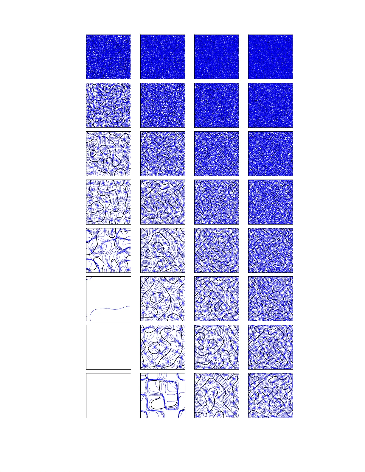
Generalised elastic nets ∗ Miguel ´ A. Carreira-P erpi ˜ n´ a n † & Geoﬀrey J. Go o dhill Departmen t of Neuroscienc e Georgetow n Univ ersit y Medical Cen ter 3900 Reserv oir Road NW, W ashington, DC 20007, US miguel@cns. georgetown.e du , geoff@georg etown.edu Abstract The elastic net w as in trod uced as a heuristic algorithm for com binatorial optimisation and has b een applied, among other problems, to biological mo delling. It has an energy fun ct ion which trades oﬀ a ﬁtn ess term agai nst a tension term. In the original form ulation of the algorithm th e tension term w as implicitly based on a ﬁrst- order deriv a tive. In this paper w e general ise the elastic net model to an arbitrary quadratic t ension term, e.g. d eriv ed from a discretised diﬀeren tial op erator, and give an eﬃcient learning algorithm. W e refer to these as generalise d elastic nets (GENs). W e give a theoretical analysis of the tension term for 1D nets with p eriodic boun dary conditions, and show that the model is sensitive to the choice of ﬁnite d iﬀerence scheme that represents the discretised deriv ative. W e il lustrate some of t h ese iss ues in the context of cortical m ap mo dels, by re lating the c hoice of tension term to a cortical interaction function. In particular, we pro ve that this intera ction takes t h e form of a Mexican hat for the original elastic net, and of progressiv ely more oscillatory Mexican hats for h igher- order deriv atives. The results app ly n ot only to generalised el astic nets b ut also to other metho ds using d iscrete diﬀerentia l p enalties, and are exp ected to b e u seful in other areas, su ch as data analysis, computer graph ics and optimisation problems. The elastic net w as ﬁrst prop osed as a metho d to obtain go o d solutions to the travelling s alesman problem (TSP; Durbin and Willshaw, 1 987) and was subse quen tly also found to b e a very successful cor tical map mo del (Durbin a nd Mitc hison, 1990; Go o dhill a nd Willshaw, 19 90; Erwin et al., 1 995; Swindale, 1996; W o lf and Geisel, 1998). Essentially , it trades oﬀ the desire to r epresent a set o f data (cities in the TSP , feature preferences in cortical ma ps) with the desire for this repr e sen tation to b e smo oth in the sens e of minimising the s um of squar ed distances of neighbouring centroids. The rela tiv e succ ess of the elastic net in these applications, its ﬂavour of wirelength minimisation, a nd its ea se of implementation, ar e proba ble reas ons why there ha s so far b een little attempt to gener alise the model be yond its orig inal form ulation, sp eciﬁcally in terms of using more co mplex tension terms. In the TSP context this is p erha ps understandable in that the or iginal tensio n term closely appr oximates the true cost, the sum o f nonsqua red dista nces (so me inv estigations of the eﬀect of using alternative exp onents for the distance function have b een per formed; Durbin and Mitch ison, 1990; Y uille et al., 1996 ). Howev er, in the c ont ext o f cor tical map mo delling the tension term repr esent s an abstra c tio n of lateral connections, who se functional for m is unknown bio logically . Although the sum-of-squa re-distances form was motiv ated as wirele ngth of neur o nal co nnections, a s sumed lar ge b et ween neurons having very dis s imilar s tim ulus preferences (Durbin and Mitc hison, 1990), this b egs the question of examining other types of tension terms to see what diﬀerence, if any , they make, as well as to rela te the tensio n term with biologically s ig niﬁcant par ameters, such as a descr iption of the intracortical co nnectivit y pattern. Day an (199 3) (see als o Y uille, 19 90; Y uille et al., 1996) was the ﬁrst to sug gest this a nd consider ed the relation of quadratic tension terms—just like those considered here—with other co r tical map mo dels. In this pa per we investigate gene r alized tension terms in mor e detail. Although our motiv ation is pr imarily bio logical, the extended mo del is also exp ected to b e gener a lly useful in a r eas s uc h as computer vision, co mputer gr a phics, imag e pro cessing , unsup e r vised lea rning a nd TSP-type problems. The pape r consists of three parts. In the ﬁrs t (sectio ns 1–2) we deﬁne the genera lised elastic net (GEN) via the int ro duction of a quadratic pe nalt y (tensio n term) in the energ y of the net and give e ﬃcie n t lear ning algor ithms for it. In the second (sections 3–5) we cons ider a class of qua dratic p enalties deﬁned as discr etised diﬀerential op erators, and give a theoretical analysis that is a pplica ble not only to genera lised ela stic nets but also to any ∗ This pap er was wr itten on August 14th, 2003 and has not b een updated since then. † Current address: Dept. of Computer Science, Unive rsity of T oronto. 6 Ki ng’s Col lege Road. T oronto, ON M5S 3H5, Canada. Email: miguel@cs. toronto.ed u . 1 mo del with a Gaussian prior . In the third part (sectio n 6) we demonstrate the r esults of the previous par ts in the problem o f cor tical map mo delling a nd rep ort additional results v ia simulation. Throughout the pa per we will often refer to the “origina l elastic net” mea ning the o r iginal formulation of the elastic net b y Durbin a nd Willshaw (1 987), with its sum-of-squar e-distances tensio n term. The equa tions for the original elastic net ar e given in section 2.6. 1 Probabilistic form ulation of the genera lised elasti c net (GEN) Given a c ollection of centroids { y m } M m =1 ⊂ R D that we expr ess as a D × M matrix Y def = ( y 1 , . . . , y M ) and a scale, or v ariance, para meter σ ∈ R + , consider a Ga ussian-mixture density p ( x | Y ; σ ) def = P M m =1 1 M p ( x | m ) with M comp onents, where x | m ∼ N ( y m , σ 2 I D ), i.e., a ll cov a riance ma trices are equal and isotropic. Consider a Gaussia n prior on the centroids p ( Y ; β ) ∝ e − β 2 tr ( Y T YS ) where β is a regular isation, or inv erse v ariance, parameter and S is a po sitive deﬁnite or p ositive semideﬁnite M × M matrix—in the latter case the prior b e ing improp er. The normalisatio n c o nstant of this densit y will no t b e relev an t for our purp oses and is given in appe ndix A. W e deﬁne a gener alise d elastic n et (GEN) by p ( x | Y ; σ ) p ( Y ; β ). The or iginal elastic net of Durbin and Willshaw (1987) and Durbin et al. (1989 ) is r ecov ered for a particular choice of the matrix S (section 2.6). It is also p oss ible to deﬁne a prior ov er the scale σ , but we will not do so here, since σ w ill play the role of the tempe rature in a deterministic annealing a lgorithm. Without the prior ov er c e n troids, the cent roids could b e per m uted at will with no change in the mo del, since the v ariable m is just an index. The prior can be used to conv ey the to p olo gic (dimension and shap e) and geometric (e.g . curv ature) str ucture of a manifold implicitly deﬁned by the cent roids (as if the cent roids were a sample from a co n tinuous latent v ariable mo del; Ca rreira- Perpi˜ n´ an, 200 1). This prio r ca n also b e seen as a Gaussian pro cess prior (e.g . Bishop et al., 1998a, p. 2 19), wher e our matrix S is the in verse of the Ga ussian pro cess cov a riance matrix. The semantics of S is not necessary to develop a lear ning algorithm and so its study is p ostp oned to section 3 . Ho wev er, it will be co n venien t to keep in mind that S will be typically der ived from a discretised deriv ative bas ed on a ﬁnite diﬀerence scheme (or stencil ) and that S will be a spars e matrix. 2 P aramet er estimation with annealing F ro m a statistical lear ning p oint of view, one might wish to ﬁnd the v alues of the par ameters Y and σ that maximise the o b jective function log p ( Y , σ | X ) = log p ( X | Y , σ ) + log p ( Y ) − log p ( X ) (1) given a training set { x n } N n =1 ⊂ R D expressed a s a D × N matrix X def = ( x 1 , . . . , x n )—that is, maximum-a-p osterior i (MAP) estimation. F or iid data and ignoring a ter m indep endent of Y and σ , this equa tion reduces to: L MAP ( Y , σ ) = N X n =1 log M X m =1 e − 1 2 k x n − y m σ k 2 − N D log σ − β 2 tr  Y T YS  . (2) How ev er, as in Durbin and Willshaw (198 7) and Durbin et al. (19 89), we are more interested in deter minis tic annealing algorithms that minimise the energy function E ( Y , σ ) def = − ασ N X n =1 log M X m =1 e − 1 2 k x n − y m σ k 2 | {z } ﬁtness te rm + β 2 tr  Y T YS  | {z } tension term (3) ov er Y alo ne, starting with a lar g e σ (for which the tensio n term dominates) a nd tracking the minim um to a small v alue of σ (for which the ﬁtness term dominates ). This is s o b ecause (1) one can ﬁnd go o d so lutions to combinatorial optimisation problems such as the TSP (which require σ → 0) and to dimension-reductio n problems such as cor tica l map mo delling (which do not requir e σ → 0 ); and (2) if co nsidered a s a dynamical system for a contin uous latent space, the evolution of the net as a function of σ and the iteration index may mo del the tempo ral evolution of cor tica l maps. T o attain go o d genera lisation to unsee n da ta, the parameter β can b e conside r ed a hyperpara meter and one ca n lo ok for an optimal v a lue for it given training data, by cr o ss-v a lidation, B ayesian inference (e.g. Utsugi, 1997 ) o r some o ther means. How ev er, in this pap er we will be interested in inv estigating the behaviour of the mo del for a ra ng e of β v alues, ra ther than ﬁxing β a c c ording to some criterion. 2 W e will ca ll the α - ter m the ﬁ tness t erm , arising from the Gaussian mixture p ( X | Y , σ ), and the β -term the tension t erm , aris ing from the prior p ( Y ). Eq. (3) diﬀers fro m the MAP ob jective function of eq. (2) in an immaterial change of sign, in the deletion of a now constant term N D log σ , and in the m ultiplication o f the ﬁtness term by ασ , where α is a po sitiv e co nstant. The latter reduces the inﬂuence of the ﬁtness term w ith resp ect to the tensio n ter m as σ decre a ses. Since α can be absor bed in β , we will take α = 1 herea fter. How ev er, it can b e useful to hav e a diﬀerent α n for each training po in t x n in order to simulate a training set that ov errepr esent s some data p oints ov er others (see section 2.5.1). W e derive three iterative alg orithms for minimising E (gra dient descent, matrix iteration and Cholesky fac- torisation), all ba sed on the gradient of E : ∂ E ∂ Y = − α σ ( XW − YG ) + β Y  S + S T 2  (4) where w e deﬁne the weigh t matrix W N × M = ( w nm ) and the inv ertible diago nal matrix G M × M = diag ( g m ) as w nm def = e − 1 2 k x n − y m σ k 2 P M m ′ =1 e − 1 2    x n − y m ′ σ    2 g m def = N X n =1 w nm . The weigh t w nm is also the resp onsibility p ( m | x n ) of centroid µ m for gener ating p oint x n , and s o g m is the total resp onsibility of c en troid µ m (or the average n umber of tra ining p oints assig ned to it). The matrix XW is then a list of av erage c e n troids. All three alg orithms, pa r ticularly the ma tr ix-iteration a nd Cho lesky-factoris ation o nes , bene ﬁt considerably from the fact that the matrix S will typically b e spa rse (with a banded or block-banded structure). 2.1 Gradien t descen t W e simply iterate Y ( τ +1) def = Y ( τ ) + ∆ Y ( τ ) with ∆ Y ( τ ) def = − σ ∂ E ∂ Y   Y ( τ ) . How ever, this only conv erges if the ratio β /α is sma ll (for large pr oblems, it needs to b e very small). F or the original elas tic net this is easily seen for a net w ith t wo centroids: the gra dien t of the tension term a t ea c h centroid p oints tow ards the other, and if the gradient step is larger than the distance b etw ee n b oth centroids, the a lgorithm diverges expo nen tially (as we hav e conﬁrmed by simulation). This could b e a lleviated by ta k ing a sho rter gra dien t step (by taking η ∆ Y ( τ ) with η < 1), but fo r lar ge β / α the step would b ecome v ery small. 2.2 Iterativ e matrix metho d Equating the gradient of eq. (4) to zero we obtain the no nlinear system Y A = XW with A def = G + σ β α  S + S T 2  . (5) This equation is similar to others obta ined under related mo delling assumptions (Y uille et al., 1 996; Day an, 1 9 93; Bishop et al., 1998b,a; Utsugi, 19 97). A is a sy mmetric po sitive deﬁnite M × M ma trix (since S is positive (semi)deﬁnite), and bo th A (through G ) and W dep end o n Y . This e q uation is the basis for a ﬁx e d- point iteration, where we so lve for Y with G and W ﬁxed, then update G and W for the new Y , a nd rep eat till conv ergence. C o n vergence is guar anteed since we can der iv e an analog ous pr oc edure as an EM algor ithm that optimises ov er Y for ﬁxed σ as in Y uille et a l. (199 4) and Utsugi (1 9 97). Essentially , eq. (5) b ecomes the familiar Gaussian-mixture up date for the means with β = 0. Th us, from the a lgorithmic p oint o f view, it is the addition of σ β α  S + S T 2  that determines the top ology . F or the clas s of matric e s S studied in this pap er, A is a large spa rse ma trix (of the order of 1 0 4 × 10 4 ) so that explicitly computing its inverse is out o f the question: b esides b eing a numerically ill-p osed op eration, it is computationally very costly in time and memory , since A − 1 is a large, nons pa rse ma tr ix. Instea d, we can solve the system fo r Y (with A a nd W ﬁxed) b y a n iterative matrix metho d (s e e e.g. Isaacso n and Keller, 19 66; Smith, 1985). Rearrang e the system (5) as Ax = b (calling x the unknowns) with A = D − L − U (diagona l − low er tria ng ular − upp er triangular ) to give an iter ative pro cedure x ( τ +1) = Cx ( τ ) + c , a few itera tions of which will usually b e enough to compute x (or Y in eq. (4)) approximately , ass uming the pro cedure conv erges. The following pro cedures are common: 3 Jacobi Decomp o sing the equa tion as Dx = ( L + U ) x + b r esults in the iterative pro cedure x ( τ +1) = D − 1 ( L + U ) x ( τ ) + D − 1 b . Since D is diagonal, D − 1 ( L + U ) can be eﬃciently c omputed a nd remains spars e. Gauss-Seidel Decomp osing the equation as ( D − L ) x = Ux + b results in the iterative pr oc e dure x ( τ +1) = ( D − L ) − 1 Ux ( τ ) + ( D − L ) − 1 b , which ca n b e implemented without explicitly co mputing ( D − L ) − 1 if instead of computing x ( τ +1) from x ( τ ) , we use the alrea dy computed elements x ( τ +1) 1 , . . . , x ( τ +1) i as w ell as the old ones x ( τ ) i +2 , . . . to compute x ( τ +1) i +1 ; see e.g . eq. (7d). Successiv e ov errelaxation (SOR ) is a lso po ssible and can be faster , but requires setting of the relaxation parameter b y tria l and err or. F or sparse matrices, b oth J acobi and Gauss-Se idel are pa rticularly fast and resp ect the spar sit y structure at e a ch iteration, without intro ducing extra nonzero elements. Both metho ds ar e quite similar, though for the k ind of sparse matrix A that we hav e with the elastic net, Gauss- Seidel should typically b e abo ut twice a s fast than Jacobi a nd r equires keeping just one copy o f Y in memory . The matr ix iterates can be interleav ed with the up dates for G a nd W . 2.3 Direct method b y Cholesky factorisation W e ca n obtain Y eﬃciently and ro bustly b y solving the spar se system of equations (5) by Gauss ian elimination via Cholesky dec o mpo s ition 1 , since A is s ymmetric a nd p ositive deﬁnite. Sp eciﬁcally , the pro cedure consists o f (George a nd Liu, 19 81; Duﬀ et a l., 19 8 6): 1. Or dering : ﬁnd a go o d p ermutation P of the matrix A . 2. Cholesky factorisation : factorise the p ermuted matr ix P AP T int o LL T where L is lo wer tr iangular with nonnegative dia gonal elements. 3. T riangular syst em solution : s olve L Y 0 = PXW and L T Y 1 = Y 0 bo th by Ga ussian elimination in O ( M ) and then set Y = P T Y 1 . Step 1 is no t str ictly nec e s sary but usua lly acceler ates the pro cedur e for sparse matrices. This is beca use, although the Cholesky factoris ation do es not a dd zer o es outside the ba nds of A (and thus pr e serves its banded structure), it may a dd new zero es inside (i.e., add new “ﬁll”), and it is p oss ible to reduce the num ber o f zer oe s in L by reorder ing the rows o f A . Howev er, the exa c t minimisa tion of the ﬁll is NP - complete and s o o ne has to use a heuristic o rdering metho d, a num b er of which exist, such a s minimum degree o r dering (Georg e and Liu, 198 1, pp. 115–13 7). 2.4 Metho d comparison The gradient descent metho d as deﬁned earlier co nverges only for β /α v a lues smaller than a cer tain thresho ld that is extremely s mall for lar ge nets; e.g. Durbin and Willshaw (1987) us e d β /α = 10 for a 2D TSP pro ble m of N = 1 00 cities a nd a net with M = 2 50 centroids; but Durbin a nd Mitc hison (1990) used β / α = 0 . 00025 for a 4D cortical map mo del of M = 1 6 00 cent roids. F o r larg e problems, a tiny r atio β /α means that—par ticularly for fast annealing—the tension ter m has very little inﬂuence o n the ﬁnal net, and a s a re sult ther e is no beneﬁt in using one matrix S ov er another. A suﬃcient co ndition fo r the convergence of b oth matrix iteratio n methods (Jacobi and Ga us s-Seidel) is that the matrix A be p ositive deﬁnite (whic h it is). Also, the Cholesky fa c torisation is stable without pivoting for all symmetric p ositive deﬁnite matrices, a lthough pivoting is adv isable for p ositive semideﬁnite matrices (Golub and v an Loan, 199 6). Thus, all three metho ds are generally appr opriate. How ever, for high v alues of β /α a nd if S is p ositive semideﬁnite, then A b ecomes numerically close to b eing p ositive semideﬁnite (even in later stages o f training, when G has larg e dia gonal elements). In this case, the Jacobi and Gauss - Seidel metho ds may diverge, a s we hav e observed in pr actice (and conv erged if β /α was lowered). In contrast, we hav e never found the Cholesky factorisatio n metho d to diverge, at least for the large st pr oblems we have tried with N , M ≈ 2 · 10 4 , D = 5, stencils o f up to order p = 4 and β /α up to 10 6 . The Cholesky facto risation is a direct metho d, computed in a ﬁnite num ber of op eratio ns O ( 1 6 M 3 ) for dense A but muc h less for s parse A . This is unlike the Jacobi or Gauss-Seidel metho ds, which are iterative and in principle 1 Da vid Wil lsha w (p ers. comm.) has also developed independently the idea of the Cholesky factorisation for the original elastic net. 4 require an inﬁnite num ber of iterations to conv erge (a lthough in pra ctice a few may be enough). With enough iterations (a few tens, for the pr o blems we tried), the Ja cobi metho d conv erges to the so lution of the Cho lesky metho d; with as few as 5 to 10 , it gets a rea sonably go o d one. In gener al, the computation time require d for the solution of eq . (5) by the Choles k y factorisa tion is usua lly ab out twice as high as that of the Ja cobi metho d. The bo ttlenec k of all ela stic net learning algorithms is the computation of the w eight matrix W of squared distances betw een cities and cen troids, which typically takes several times longer than solving eq. (5). Thus, using the Cholesky factorisatio n o nly means an increase of ar ound 10– 20% of the to tal computation time. Regarding the quality of the itera tion, the Cholesk y metho d (and, for enough itera tions, the Jac o bi and Gauss- Seidel metho ds) go es deep er down the energy surface a t each annealing iteration; this is par ticularly noticea ble when the net collapses into its centre of mass for large σ . In contrast, gradient descent ta kes tiny steps and r e quires many mor e iterations for a no tice a ble change to o ccur. It might then b e p ossible to use faster annealing than with the gradient metho d, with considera ble sp eedups. On the other hand, the Cholesky metho d is not appro pr iate for online lea rning, where training p oints come one at a time, b ecause the net w ould change dra stically fr om one training p oint to the next. How ever, this is not a pr oblem practically since the stream of da ta can a lways b e split int o c hunks o f a ppropriate size . In summary , the ro bus tness and eﬃciency of the (spars e ) Cholesky fa ctorisation make it our metho d of choice and allow us to inv estigate the b ehaviour of the mo del for a larg er r ange of β v alues than has pr eviously b een po ssible. All the simulations in this pap er use this method. 2.5 Practical ext ensions Here we descr ibe tw o pr a ctically conv enient mo diﬁcations of the ba sic elas tic net mo del. 2.5.1 W eighting p oi nts o f the traini ng set F or some applications it may b e conv enien t to deﬁne a separate α n ≥ 0 for ea ch data p oint x n (e.g. to overrepresent some data p oints without having to add e xtra copies of each p oint, which would make N larger). In this case , the energy b ecomes E ( Y , σ ) = − σ N X n =1 α n log M X m =1 e − 1 2 k x n − y m σ k 2 + β 2 tr  Y T YS  and a ll o ther equatio ns remain the sa me by deﬁning the w eights as w nm def = α n e − 1 2 k x n − y m σ k 2 P M m ′ =1 e − 1 2    x n − y m ′ σ    2 = α n p ( m | x n ) , that is, multiplying the old w nm times α n . Over- o r underrepr e sen ting training set p oints is useful in cortical map modelling to s imulate depr iv ation conditions (e.g. mono cular depriv a tion, b y reducing α n for the p oints a sso ciated with one eye) or nonuniform feature distributions (e.g. cardinal or ient ations are ov errrepr esent ed in natural images). It is als o po ssible to make α n depe ndent on σ , so that e .g . the ov errepresentation may take pla ce at s peciﬁc times during lear ning; this is useful to mo del critical pe rio ds (Car reira-Perpi ˜ n´ an et al., 2003). 2.5.2 In tro ducing zero-v alue d mixing prop o rtions W e deﬁned the ﬁtness term o f the elastic net as a Gaus sian mixture with equipro bable comp onents. Instea d, we ca n asso ciate a mixing prop ortio n π m def = p ( m ) with each co mponent m , sub ject to π m ∈ [0 , 1] ∀ m a nd P M m =1 π m = 1. In an unsup ervised learning setting, w e could ta ke { π m } M m =1 as parameters a nd learn them from the training set, just as we do with the centroids { y m } M m =1 . How ever, we can also use them to dis a ble cen troids from the mo del selectively during tra ining (b y setting the cor resp onding π m to zero). This is a co mputationally conv enien t s trategy to use non-re c tangular grid shap es in 2D nets. Sp eciﬁcally , for each comp onent m to b e disabled, we need to: • Set π m = 0 (and re no rmalise all π m ). • If using a s y mmetric matrix S = D T D , set to zer o column m o f D a nd all r ows m ′ of D that had a nonzero in the element corresp onding to column m . This is equiv alent to eliminating from the tens ion term all linear combinations that inv olved y m . This implicitly as sumes a sp eciﬁc t yp e o f b oundary c o ndition; other 5 t yp es of b.c. may b e used by appropria tely mo difying such r ows (r ather than zeroing them). If S is not symmetric, the manipula tions ar e more complicated. It is easy to see that the energ y is now indep endent of the v alue of y m : no “force” is exerted on y m either from the ﬁtness o r the tensio n term, and likewise y m exerts no tens io n on a n y other centroid. Th us, in the training algorithm, we ca n s imply r emov e it (and the appro priate pa r ts of S , etc.) from the up date equations . W e could also simply leav e it there, since its g radient comp onent is zero a nd its a sso ciated equation (5) is zero b oth in the RHS and the LHS (for all d = 1 , . . . , D ). Howev er, the latter option is computationally wasteful, since the op erations a sso ciated with y m are still b eing car ried out, and can lead to n umerical instability in the iterative- matrix and Chole sky-factorisa tion metho ds, since the matrices inv olved b ecome singular (although this can b e easily ov ercome by setting g m to some no nzero v alue). When mix ing prop or tions π m and training set weigh ts α n are used, the energy bec o mes: E ( Y , σ ) = − σ N X n =1 α n log M X m =1 π m e − 1 2 k x n − y m σ k 2 + β 2 tr  Y T YS  and a ll o ther equatio ns remain the sa me by deﬁning the w eights as w nm def = α n π m e − 1 2 k x n − y m σ k 2 P M m ′ =1 π m ′ e − 1 2    x n − y m ′ σ    2 = α n p ( m | x n ) . Selectively disabling centroids is useful in cortical map mo delling to use a 2 D net that approximates the shap e of primary vis ual cortex and may include les io ns (patches of inactive neurons in the cortex ). It c a n also b e used to train separate nets on the s ame training set and s o force them to comp ete with ea ch other (both with 1D or 2D nets); in fact, the central-diﬀerence stencil (section 5.5.2) leads to a similar situa tion by separ ating the tension term in to de c o upled subterms. 2.6 Comparison with the original elastic net mo del The origina l elastic net results from using the matrix D co rresp onding to a stencil (0 , − 1 , 1) and S = D T D (see section 4 ). F or example, for a 1D net with M = 9 centroids (where a = 0 for nonp erio dic b.c. and a = 1 for per io dic b.c.): D =       − 1 1 0 0 0 0 0 0 0 0 − 1 1 0 0 0 0 0 0 0 0 − 1 1 0 0 0 0 0 0 0 0 − 1 1 0 0 0 0 0 0 0 0 − 1 1 0 0 0 0 0 0 0 0 − 1 1 0 0 0 0 0 0 0 0 − 1 1 0 0 0 0 0 0 0 0 − 1 1 a 0 0 0 0 0 0 0 − a       S =       a 2 +1 − 1 0 0 0 0 0 0 − a 2 − 1 2 − 1 0 0 0 0 0 0 0 − 1 2 − 1 0 0 0 0 0 0 0 − 1 2 − 1 0 0 0 0 0 0 0 − 1 2 − 1 0 0 0 0 0 0 0 − 1 2 − 1 0 0 0 0 0 0 0 − 1 2 − 1 0 0 0 0 0 0 0 − 1 2 − 1 − a 2 0 0 0 0 0 0 − 1 a 2 +1       . (6) W e obtain the original ela stic net equations (Durbin and Willshaw, 1 987; Durbin et al., 1989) as follows: Energy: E ( Y , σ ) = − ασ N X n =1 log M X m =1 e − 1 2 k x n − y m σ k 2 + β 2 M X m =1 k y m +1 − y m k 2 (7a) Gradient: ∆ y m = α N X n =1 w nm ( x n − y m ) + β σ ( y m +1 − 2 y m + y m − 1 ) (7b) Jacobi: y ( τ +1) m = α P N n =1 w nm x n + β σ ( y ( τ ) m +1 + y ( τ ) m − 1 ) α P N n =1 w nm + 2 β σ (7c) Gauss-Seidel: y ( τ +1) m = α P N n =1 w nm x n + β σ ( y ( τ ) m +1 + y ( τ +1) m − 1 ) α P N n =1 w nm + 2 β σ . (7d) The original e la stic net pa per s used annealing with either gradient de s cen t (Durbin a nd Willshaw, 1987; Durbin et al., 1 989) or Gauss -Seidel iteration (Durbin and Mitc hison, 1990 ). F or the latter, the up dates o f y 1 , . . . , y m m ust be do ne sequentially on the index m . 6 3 Construction of the matrix S The deﬁnition of the mo del and the optimisation alg orithms given dep end on the matrix S ; we ar e left now with the sea r ch for a meaningful matrix S that incorpo rates some knowledge o f the problem being mo delled. F or example, for the original e la stic net, the tension term embo dies a n approximation to the leng th o f the net, which is the basis for a heuristic solution of the TSP a nd for a cortical ma p mo del. In this section we discuss genera l prop erties of the matrix S and then, in the next section, co ncen trate on diﬀerential op erato rs. Firstly , note that the for m ulation of the tensio n term (ignoring the β / 2 fa c tor) a s tr  Y T YS  = P m,m ′ ,d s mm ′ y dm y dm ′ is not the most general quadratic form of the par ameters { y dm } M ,D m,d =1 . This is b ecause the cross-ter ms y dm y d ′ m ′ for d 6 = d ′ hav e weight zer o and the terms y dm y dm ′ hav e a weigh t s mm ′ independent o f the dimensio n d . Thu s, the diﬀerent dimensions of the net d = 1 , . . . , D (or maps) are independent and formally iden tical in the tension term (thoug h not so in the ﬁtness term). The most general quadratic form could b e repr esented as vec ( Y ) T S vec ( Y ) where vec ( Y ) is the co lumn co ncatenation of all elements of Y and S is now M D × M D , or as P m,m ′ ,d,d ′ s mdm ′ d ′ y md y m ′ d ′ where s mdm ′ d ′ is a 4D tenso r. How ever, our mor e particular class o f p enalties still has a rich b ehaviour and we r estrict o urselves to it. Secondly , note that it is enoug h to co nsider symmetric matrices S o f the form D T D where D is arbitrar y . W e hav e that, for a nonsymmetric matrix S : tr  Y T Y  S + S T 2  = 1 2  tr  Y T YS  + tr  Y T YS T  = 1 2  tr  Y T YS  + tr  ( Y T YS T ) T  = tr  Y T YS  and so using S is equiv alent to using the symmetric form S + S T 2 . F urther, since S m ust b e po sitiv e (se mi)deﬁnite for the energy to b e low er b ounded, we can always wr ite S = D T D for some real D matrix, without loss of generality , and so the tension ter m can b e wr itten tr  Y T YS  =   D Y T   2 where k A k def = p tr ( A T A ) = q P ij a 2 ij is the F rob enius matrix norm. How ev er, the lear ning algorithms given ea rlier can b e used for any S . The D matrix has tw o functions. As neighb ourho o d r elation , it sp eciﬁes the streng th of the tension b et ween centroids and thus the expected metric pr op erties of the net, such as its curv ature. As adjac ency matrix , it sp eciﬁes what centroids are directly connected 2 and so the top olo gy o f the net. Th us, by changing D , w e can turn a given collectio n of centroids into a line, a closed line, a plane sheet, a torus, etc. Pr actically , we typically concern o urselves with a ﬁxed top olog y and are interested in the eﬀects of changing the “elas ticity” or “stiﬀness” of the net via the tension ter m. Thirdly , for net top olo gies wher e the neighbo urho o d rela tions do not dep end on the actual r egion in question of the net, we can repr esent the matrix D in a compact form via a stencil and suitable bo undary conditions (b.c.). Multiplicatio n by D then b ecomes c o n volution by the stencil. F urther, in sec tio n 5.6 we will show that with perio dic b.c. we can alwa ys take D to b e a symmetr ic matrix and so S = D 2 . In summary , we ca n re present quadratic tension terms in full generality through an op era to r matrix D , and we will concentrate on a par ticular but impo rtant cla ss of ma trices D , w he r e diﬀerent dimensions are indep endent and ident ical in form, and where the op erator is a ssumed translationally in v ar iant so that D results from conv olving with a stencil. Before c o nsidering appr opriate types of stencil, we note so me imp ortant inv a riance prop erties . 3.1 In v ariance of the p enalty term wit h resp ect to rigid motions of the net Consider a n o rthogonal D × D matr ix R a nd a n ar bitr ary D × 1 vector µ . In order that the matrix D repres en t an o p era tor inv ariant to ro ta tions and transla tions o f the net centroids, we must hav e the same p enalty for Y and for R ( Y + µ 1 T ) (where 1 is the M × 1 vector of ones): tr  Y T YD T D  = tr  ( Y + µ 1 T ) T R T R ( Y + µ 1 T ) D T D  = tr  Y T YD T D  + tr  Y T µ 1 T D T D  + tr  1 µ T YD T D  + tr  1 µ T µ 1 T D T D  . Thu s, any D will provide inv aria nce to r otations, but inv a riance to translatio ns requir es D1 = 0 , i.e., a diﬀerential op erator ma trix D (see later). Another wa y to s e e this, for the circula n t matr ix case discussed later , is as follows: a circulant p ositive de ﬁnite matrix S = D T D can always b e decomp osed as ˜ S + k 11 T with ˜ S cir culant p ositive semideﬁnite (verifying ˜ S1 = 0 , or P M m =1 ˜ s 1 m = 0) and k = 1 M 2 1 T S1 = 1 M P M m =1 ˜ s 1 m > 0. This corres ponds to the pr o duct o f tw o prio r s, o ne 2 How ever, the notion of adjacency b ecomes blurred when we consider that a spars e stencil such as (0 , − 1 , 1) can be equiv alen t (i.e., pro duce the same S ) to a nonsparse one, as we sho w in section 5.6. 7 given by the diﬀerential op erato r matr ix ˜ S and the other one by the matrix k 11 T . The eﬀect of the latter is to pena lis e non-zer o-mean nets, since tr  Y T Y ( k 11 T )  = k P D d =1 ( P M m =1 y dm ) 2 , which we do not want in the present context, since it dep ends on the choice o f o rigin for the net. Such matrice s ca n b e des irable for smo othing applications, na turally , and the training a lg orithms still work in this cas e b ecause S remains p o sitive s e mideﬁnite (and so the energ y function is bo unded b elow). 3.2 In v ariance of S with respect to transformations of D or the stencil There can b e diﬀerent matrices D that result in the sa me S = D T D ; in fact, D T is a squar e ro ot o f S . Any matrix D ′ def = RD will pro duce the sa me S if R is a k ′ × k matrix verifying R T R = I k . This is the same s ort of uniden tiﬁability as in factor analy s is (by rotation of the factor s; Bartholo mew, 1987), and in our ca se it means that the same nonneg ative quadra tic form can b e obtained for many diﬀerent ma trices D . Particular cases inc lude: • Orthogona l ro ta tion of D : R is square w ith R − 1 = R T . • Sign re versal of any num ber of rows o f D : R is diago nal with ± 1 e le ments. • Perm utation of rows of D (i.e., reo r dering of the summands in the tension term): R is a p ermutation matr ix . • Insertion of rows of zero es to D : R = R k ′ × k is the ide ntit y I k with k ′ − k intercalated r ows of zero es. When D is derived from a stencil, S is inv ariant with res p ect to the fo llowing stencil trans formations: • Sign re versal, e.g. (1 , − 2 , 1) is equiv alent to ( − 1 , 2 , − 1). • Shifting the stencil, s ince this is equiv alent to p ermuting rows of D . In pa rticular, padding with zer o es the bo rders of the stencil (but not inser ting zero es), e.g. the forward diﬀerence (0 , − 1 , 1) is equiv alen t to the backw ard diﬀere nce ( − 1 , 1 , 0 ) but not to the central diﬀerence ( − 1 , 0 , 1). These inv ariance prop erties are useful in the a na lysis o f s e ction 5 and in the implemen tation of co de to co ns truct the matrix S given the stencil. 4 Construction of the matrix D from a diﬀeren tial stencil ς T o represent the matrix D by a stencil co nsider for example the origina l elastic net, in which the tension term con- sists of summing ter ms of the form k y m +1 − y m k 2 ov er the who le net. In this case, the stencil is (0 , − 1 , 1) a nd con- tains the coe ﬃcie n ts that multiply y m − 1 , y m and y m +1 . In g eneral, a s tencil ς = ( ς − k , ς − k +1 , . . . , ς 0 , . . . , ς k − 1 , ς k ) represents a linear combination P k i = − k ς i y m + i of which then we take the s q uare. A given row of matr ix D is obtained by cen tring the stencil on the corresp onding column, and successive rows by shifting the stencil. If the stencil is sp arse , i.e., has few nonzer o elements, then D and S are spar se (with a banded or blo ck-banded structure). It is nece ssary to sp ecify b oundary co nditio ns when one of the stencil ends overspills near the net b oundar ie s . In this pap er we will consider only the simplest t ype s of b oundar y conditions : p erio dic , which uses mo dular arithmetic; and nonp erio dic or op en , which simply disca rds linea r combinations (rows of D ) that ov erspill. In bo th ca ses the resulting D ma trix is a structured matr ix : circulant for per iodic b.c., s ince it is obtained by successively ro tating the stencil (see sec tio n 5); or quasi-T o eplitz for nonp erio dic b.c., b eing almost c o mpletely deﬁned by its top r ow and left column. The following exa mple illustrates these ideas for a stencil ς = ( a, b , c, d, e ) and a 1 D net with M = 7 : Nonpe rio dic b.c.: D =  a b c d e 0 0 0 a b c d e 0 0 0 a b c d e  Periodic b.c.: D =    c d e 0 0 a b b c d e 0 0 a a b c d e 0 0 0 a b c d e 0 0 0 a b c d e e 0 0 a b c d d e 0 0 a b c    Y T =    y T 1 y T 2 . . . y T 7    . These ideas generalise dir ectly to elas tic nets of tw o or more dimensions, but the structure of D is more compli- cated, b eing cir c ulan t or quasi-T o eplitz by blo cks. In the a nalysis of sectio n 5 we consider o nly p erio dic b.c. for simplicity , but the examples of se c tion 6 will include b oth perio dic and nonp erio dic b.c. Some notational rema rks. As in the earlier example, we will ass ume the conv en tion tha t the ﬁr s t r ow of D contains the stencil with its central co eﬃcie nt in the ﬁrst column, the co eﬃcients to the right of the stencil o ccupy columns 2 , 3, etc. of the matr ix and the co eﬃcients to the left o ccup y co lumns M , M − 1, etc. r espe c tiv ely . The 8 remaining rows of D are obta ine d by succe ssively rota ting the stencil. Without loss of genera lit y , the stencil m ust hav e an o dd nu mber of elements to av oid ambiguit y in the as signation of these elements to the net p oints. Occasiona lly we will index the stencil starting fro m the left, e.g. ς = ( ς 0 , ς 1 , ς 2 , ς 3 , ς 4 ). W e will always assume that the num ber of centroids M in the net (the dimension of the vector y ) is lar ger than the num ber of co eﬃcients in the stencil and s o will often need to pad the stencil with zero es. Rather than explicitly notating all these circumstances, which would b e cumbers o me, we will make clear in each context which version of the indexing we are using . This conv en tion will make easy v arious o per a tions we will need la ter, such as rotating the stencil to build a circ ulan t matrix D , conv olving the s tencil with the net or computing the F ourier tra nsform o f the stencil. The tension term s eparates additively into D terms, one for each r ow of Y , so we cons ider the case D = 1; call y def = Y T the resulting M × 1 vector. In this formulation, the vector D T y is the discrete convolution of the net and the stencil, while the vector Dy (which is what we use) is the discre te convolution o f the net and the r everse d stencil ← − ς def = ( . . . ς 2 , ς 1 , ς 0 , ς − 1 , ς − 2 . . . ). In b oth cases the tension v alue is the s ame. This can be readily s een by noting that P M k =1 d ki d kj = P M k =1 d ik d j k if D is circulant, which implies D T D = DD T and so   D Y T   2 =   D T Y T   2 ; or by noting that the stencil and the reverse stencil hav e the same p ow er sp ectrum ( | ˆ ς k | 2 = | ˆ ← − ς k | 2 ). 4.1 T yp es of discretised oper ator T urning now to the choice of stencil, there are t wo ba sic types: Diﬀerent ial, o r roug hening This results when the stencil is a ﬁnite-diﬀerence approximation to a contin uous diﬀerential op e rator, such a s the forward diﬀere nce a pproximation to the ﬁr st der iv ative (Cont e a nd de Bo or, 1980): y ′ ( u ) ≈ y ( u + h ) − y ( u ) h = ⇒ ς = (0 , − 1 , 1 ) where the grid co nstant h is small. Diﬀeren tial o p era tors characterise the metric prop erties of the function y , such as its curv ature, and are lo c al , their v alue b eing given at the p oint in question. Consequently , the algebraic sum of the elements of a ﬁnite-diﬀerence stencil m ust b e zero (otherwise, the o per ator’s v alue v alue would diverge in the contin uum limit, as h → 0). This zer o-su m c ondition can also b e expressed as D1 = 0 , where 1 is a vector of ones, and ha s the co nsequences tha t: D is rank-defective (having a zero eigenv alue with eigenv ector 1 ); S is p ositive s emideﬁnite and the prior on the centroids is improp er; a nd the tension term is in v ar iant to rigid motions of the centroids (tra nslations and rota tions). No te the ﬁtness term is inv aria nt to per m utations of Y but not to r igid motions . In tegral, or smo o thing This results when the stencil is a Newton-Co tes quadra tur e formula, such a s Simpson’s rule (Co n te and de Bo or, 1980): Z u +2 h u y ( v ) dv ≈  y ( u ) + 4 y ( u + h ) + y ( u + 2 h ) 3  h = ⇒ ς = 1 3 (0 , 0 , 1 , 4 , 1) . Int egral op erators are not lo c al , their v alue being given by a n in terv a l. Thus, the corr esp o nding stencil is not zer o-sum. Int egral op erator s dep end on the choice o f or ig in (i.e., the “DC v a lue”) and so do not seem useful to co nstrain the geometric form of an e la stic net, nor would they hav e an obvious biolog ic al interpretation (altho ug h, of co urse, they a re use ful as smo othing op erator s). Diﬀerential op erator s, in contrast, can b e readily in terpreted in ter ms of con tinuit y , smo othness and other geo metric pro per ties of curves—whic h a r e one of the generally accepted principles that gov ern cortical maps, together with uniformity of cov erage of the stimuli s pace (Swindale, 19 91, 1996; Swindale et al., 2 0 00; Car reira-Perpi ˜ n´ an and Go o dhill, 2 002). Note that the eﬀect of the tension ter m is opp osite to that of the o per ator, e.g. a diﬀerent ial op erator will res ult in a pena lt y for nonsmo oth nets. Also, let us br ieﬂy consider a prio r that is particularly simple a nd e asy to implemen t: S = I , or a tensio n term pr opo rtional to P md y 2 md , resulting fr o m a stencil ς = (1). By placing it on the pa rameters of a mapping, this prior has often b een used to reg ularise mappings , as in neur al nets (weigh t decay , or ridge r egressio n; Bishop, 1995) or GTM (Bishop et a l., 1 998b). In these cases , s uc h a prior p erfor ms w ell b ecause even if the weights are forced to small mag nitudes, the cla ss of functions they repres en t is still la rge and so the da ta ca n b e mo deled well. In contrast, in the elastic net the prior is no t on the weight s of a pa rameterized mapping but on the v alues o f the mapping itself, and so the eﬀect is disastr ous: ﬁrs t, it biases the centroids tow ards the o rigin irr espec tively of 9 the lo cation of the training set in the co or dinate system; seco nd, there is no top olog y b ecause the prio r factoriz es ov er all y md . W e now concentrate on diﬀer ential stencils, i.e., P n ς n f n will appr oximate a g iv en deriv ativ e o f a co ntin uous function f ( u ) thr o ugh a regular ly spa ced sample o f f . In essence, the stencil is just a ﬁnite diﬀerence scheme. Particular cases of such diﬀerential o per a tors have been applied in related work. Day an (1993 ) prop osed to construct top olog y matric e s by se lecting diﬀerent ways of reco nstructing a net no de from its neighbo ur s (via a matrix E ). This strategy is equiv alen t to using a D matrix deﬁned as D = I − E . F or the ex amples he used, E = (0 , 0 , 1) co rresp onds to D = ( − 1 , 1 , 0) (the original elastic net: forward diﬀerence of order 1); and E =  1 2 , 0 , 1 2  corres p onds to D =  − 1 2 , 1 , − 1 2  (forward diﬀerence of o rder 2). The la tter was also used by Utsugi (19 97) and Pascual- Marqui et al. (200 1). Here we seek a more systematic wa y o f deriving stencils that approximate a deriv a tiv e of order p . T ables 1-2 give s everal ﬁnite-diﬀerence s c hemes for functions (nets) o f one and tw o dimensio ns, resp ectively . 4.2 T runcation error of a diﬀeren t ial stencil Metho ds for obtaining ﬁnite-diﬀerence schemes such as truncated T aylor ex pansions (the metho d of undeter mined co eﬃcient s), interp olating po lynomials or symbolic techniques can b e found in numerical analys is textb o oks (see e.g. Co n te and de Bo or, 19 80, section 7.1; Gerald and Wheatley, 19 94, chapter 4 and app endix B; Go dunov and Ryaben’ki ˘ ı, 1987 , § 11.6 ). Here w e consider T aylor expansions. Given a diﬀere ntial s tencil ς , w e can de ter mine what deriv a tive it approximates and c ompute its trunca tion err or by using a T aylor expansio n aro und u : f ( u + mh ) = R X r =0 f ( r ) ( u ) ( mh ) r r ! + f ( R +1) ( ξ ) ( mh ) R +1 ( R + 1)! m ∈ Z , ξ ∈ ( u, u + mh ) . Consider a centre-aligned stencil ς = ( . . . , ς − 1 , ς 0 , ς 1 , . . . ) and deﬁne ← − ς ( u ) = P m ← − ς m δ ( u − m h ) ov er R where ← − ς m = ς − m . Then: ( ← − ς ∗ f )( u ) = Z ∞ −∞ X m ← − ς m δ ( v − mh ) f ( u − v ) dv = X m ς − m Z ∞ −∞ δ ( v − mh ) f ( u − v ) dv = X m ς − m f ( u − mh ) = X m ς m f ( u + mh ) = R X r =0 α r h r f ( r ) ( u ) + α R +1 h R +1 f ( R +1) ( ξ ) with α r = 1 r ! X m ς m m r . (8) Call p a nd q the sma llest integers such that α p , α q 6 = 0 and α r = 0 for r < p a nd p < r < q . Then, doing q = R + 1 gives f ( p ) ( u ) = ( ← − ς ∗ f )( u ) α p h p + ǫ ( h ) with ǫ ( h ) def = − f ( q ) ( ξ ) α q α p h q − p (9) where ξ is “near” u . That is, ς repr esents a der iv ative of o rder p with a truncation erro r ǫ ( h ) of o rder q − p ≥ 1 (note that for any diﬀerential s tencil p ≥ 1 and so α 0 = P m ς m = 0 , the zer o-sum condition). Co nversely , to construct a stencil that approximates a de r iv ative of order p with truncation error of or der q − p we simply solve for the co eﬃcients ς m given the v alues α r . Obviously , a de r iv ative of order p can b e approximated by many diﬀerent stencils (with diﬀerent or the sa me truncation er ror). F rom a nu merical analysis p oint of view, one seeks stencils that hav e a high err or order (so that the approximation is mor e accur ate) and as few nonzero co eﬃcients as p oss ible (so that the conv olution ← − ς ∗ f can b e eﬃciently computed); for example, for the ﬁrst-o rder deriv ative the central-diﬀerence stencil  − 1 2 , 0 , 1 2  , which has quadratic error , is preferable to the forward-diﬀerence stencil (0 , − 1 , 1), which has linear erro r—in fact, the ce ntral diﬀerence is routinely used b y ma thema tical soft ware to approximate gr adient s. How ev er, from the p oint of view of the GE N, the nonuniqueness o f the stencil r aises an imp ortant question: can we exp ect diﬀerent stencils o f the same deriv ative o rder to b ehav e similarly? Surprisingly , the answer is no (see se c tio n 5 .5). Before pr oc eeding, it is imp ortant to make a clariﬁca tio n. It is well known that e stimating der iv atives from noisy data (e.g. to lo cate edges in an imag e) is an ill-p osed pro blem. The deriv atives we compute are not ill-p osed bec ause the net (given b y the loc ation of the centroids) is no t a no isy function—the v alue of the tensio n ter m is computed exactly . 10 Order p Stencil × h p Erro r ter m Key 1 (0 , − 1 , 1) − y ′′ ( ξ ) h 2 1A 1 ( − 1 , 1 , 0) y ′′ ( ξ ) h 2 1A 1 1 2 (0 , 0 , − 3 , 4 , − 1) y ′′′ ( ξ ) h 2 3 1C 1 1 2 ( − 1 , 0 , 1) − y ′′′ ( ξ ) h 2 6 1B 1 1 12 (0 , 0 , 0 , 0 , − 25 , 48 , − 36 , 16 , − 3) y v ( ξ ) h 4 5 1D 1 1 12 (0 , 0 , − 3 , − 10 , 1 8 , − 6 , 1) − y v ( ξ ) h 4 20 1E 1 1 12 (1 , − 8 , 0 , 8 , − 1) y v ( ξ ) h 4 30 1F 1 1 60 (0 , 0 , 2 , − 24 , − 3 5 , 80 , − 3 0 , 8 , − 1 ) y vii ( ξ ) h 6 105 1G 1 1 60 ( − 1 , 9 , − 45 , 0 , 4 5 , − 9 , 1 ) − y vii ( ξ ) h 6 140 1H 2 (0 , 0 , 1 , − 2 , 1 ) − y ′′′ ( ξ ) h 2A 2 (0 , 0 , 0 , 2 , − 5 , 4 , − 1) y iv ( ξ ) 11 h 2 12 2C 2 1 4 (1 , 0 , − 2 , 0 , 1) − y iv ( ξ ) h 2 3 2B 2 (1 , − 2 , 1) − y iv ( ξ ) h 2 12 2A 2 1 12 (0 , 0 , 0 , 0 , 35 , − 104 , 114 , − 56 , 1 1 ) − y v ( ξ ) 5 h 3 6 2D 2 1 12 (0 , 0 , 1 1 , − 20 , 6 , 4 , − 1) y v ( ξ ) h 3 12 2E 2 1 12 ( − 1 , 16 , − 30 , 16 , − 1) y vi ( ξ ) h 4 90 2F 2 1 180 (0 , 0 , − 13 , 2 28 , − 420 , 2 00 , 15 , − 12 , 2) − y vii ( ξ ) h 5 90 2G 2 1 180 (2 , − 27 , 2 70 , − 490 , 2 70 , − 27 , 2) − y viii ( ξ ) h 6 560 2H 3 (0 , 0 , 0 , − 1 , 3 , − 3 , 1) − y iv ( ξ ) 3 h 2 3A 3 1 8 ( − 1 , 0 , 3 , 0 , − 3 , 0 , 1) − y v ( ξ ) h 2 2 3B 3 1 2 ( − 1 , 2 , 0 , − 2 , 1) − y v ( ξ ) h 2 4 3C 3 1 2 (0 , 0 , − 3 , 10 , − 12 , 6 , − 1) y v ( ξ ) h 2 4 3D 3 1 8 (0 , 0 , − 1 , − 8 , 35 , − 48 , 29 , − 8 , 1) − y vii ( ξ ) h 4 15 3E 3 1 8 (1 , − 8 , 13 , 0 , − 13 , 8 , − 1) y vii ( ξ ) 7 h 4 120 3F 4 (0 , 0 , 0 , 0 , 1 , − 4 , 6 , − 4 , 1 ) − y v ( ξ )2 h 4A 4 (1 , 0 , − 4 , 0 , 6 , 0 , − 4 , 0 , 1 ) − y vi ( ξ ) 2 h 2 3 4B 4 (1 , − 4 , 6 , − 4 , 1) − y vi ( ξ ) h 2 6 4A 4 1 6 ( − 1 , 1 2 , − 39 , 5 6 , − 39 , 1 2 , − 1) y viii ( ξ ) 7 h 4 240 4C T able 1: A galler y of 1D discretised diﬀerential o p era tors obtained from ﬁnite diﬀerence schemes. y is a 1D function of a 1D indep endent v ariable u ev aluated at p oint s in a regular grid with interpoint separation h def = u m +1 − u m , so that y m def = y ( u m ), and ξ is a n unknown p oint near u m . The key in the la s t column r e fers to ﬁgur e 4. Example: for 3 A we have y ′′′ m = y m +3 − 3 y m +2 +3 y m +1 − y m h 3 − y iv ( ξ ) 3 h 2 . 5 Analysis of the tension term in 1D W e hav e a way of constructing stencils (or conv olution kernels) tha t r e present a n arbitra ry diﬀerential o p era tor, and from a stencil the corr espo nding D ma tr ix that repres en ts the discre te c o n volution with the net. The tension term v alue is then the summed v alue in norm L 2 of this conv olution. In this section we theoretica lly analyse the character of the diﬀerent stencils. W e b egin by comparing the discrete net with the contin uum limit and noting 11 Order p Op era tor Stencil × h p Erro r term Key 2 Laplacian ∇ 2 y  1 1 − 4 1 1  O ( h 2 ) ∇ 2 + 2 Laplacian ∇ 2 y 1 2  1 1 − 4 1 1  O ( h 2 ) ∇ 2 × 2 Laplacian ∇ 2 y 1 6  1 4 1 4 − 20 4 1 4 1  O ( h 6 ) ∇ 2 9 2 Laplacian ∇ 2 y 1 12 − 1 16 − 1 16 − 60 16 − 1 16 − 1 ! O ( h 4 ) ∇ 2 a 4 Biharmonic ∇ 4 y 1 2 − 8 2 1 − 8 20 − 8 1 2 − 8 2 1 ! O ( h 2 ) ∇ 4 a 4 Biharmonic ∇ 4 y 1 6    − 1 − 1 14 − 1 − 1 20 − 77 20 − 1 − 1 14 − 77 184 − 77 14 − 1 − 1 20 − 77 20 − 1 − 1 14 − 1 − 1    O ( h 4 ) ∇ 4 b T able 2: A gallery of 2D discretised diﬀerential o per ators obtained fro m ﬁnite diﬀerence schemes. y is a 1 D function of a 2D indep endent v a riable u ev aluated a t p oints in a r e g ular squa re grid with int erp oint separatio n h def = k u i +1 ,j − u ij k = k u i,j +1 − u ij k , so that y ij def = y ( u ij ). The 2D La pla cian op era tor is ∇ 2 y def = ∂ 2 y ∂ u 2 1 + ∂ 2 y ∂ u 2 2 and the 2D bihar monic op erator is ∇ 4 y def = ( ∇ 2 ) 2 y = ∂ 4 y ∂ u 4 1 + 2 ∂ 4 y ∂ u 2 1 ∂ u 2 2 + ∂ 4 y ∂ u 4 2 . The key in the las t column refers to ﬁgure 6 . Example: for ∇ 2 + we have ∇ 2 y ij = y i +1 ,j + y i − 1 ,j + y i,j +1 + y i,j − 1 − 4 y ij h 2 + O ( h 2 ). Z ero-v alued co eﬃcients a r e omitted in the stencil repr esent ation. the e xtra deg ree o f freedom that the choice of stencil introduces in the discr ete cas e as opp osed to the unique deﬁnition of deriv ative in the contin uous o ne. The subsequent analy sis is based on the F our ie r s p ectrum of the stencil (or equiv a le ntly the eigensp ectrum of the S ma tr ix) for the case o f circulant matrice s D (i.e., p erio dic b.c.). W e characterise the behaviour o f families of stencils , based on the forward and central diﬀere nce, resp ectively , and show how the former but not the latter ma tc hes the b ehaviour in the contin uous case. In particula r, we show that the frequency conten t of the net (the strip e width for cortical ma ps) mov es tow ards higher frequencies as the stencil orde r incr eases in the forward-diﬀerence family , while for the central-diﬀerence family the net has the highest frequency for any or der. W e also show tha t the diﬀerent stencils can b e rewritten as Mexican- ha t kernels with prog ressively mor e o scillations as the order increa ses. In pa rticular, this mea ns that the original elas tic net, motiv ated by wirelength a rguments, is eq uiv alent to an excitator y-inhibitory Mexican hat. F or the mo st part, we will consider 1D nets for simplicity , a lthough many of the results c arry over to the L -dimensional case. While the b ehaviour of the GEN is given by the joint eﬀect of the ﬁtness and tension terms o f its energ y function, a separate a nalysis of the tensio n term g ives insight into the character of the minima of the energy . Besides, it makes e xplicit the diﬀerences b etw ee n the contin uous and the discrete for m ulations of the net. 5.1 Con tin uous case vs discrete case Let us c o nsider the tension term of the energy function (3) o f the GEN with S def = D T D and a gain ignor ing the β 2 factor, tr  Y T YS  =   D Y T   2 . Consider a 1 D co ntin uous net y ( u ) def = ( y 1 ( u ) , . . . , y D ( u )) T ∈ R D depe nding on a contin uous v ariable u that takes v a lues in R . W e ca n express the tension term a s a sum of D terms, one for each function y d , where each term is of the for m: Z ∞ −∞ ( D y ( u )) 2 du = kD y k 2 2 (10) where k·k 2 is the L 2 -norm in the space of s quare-integrable functions. D repr esents a linear diﬀerential op erator, such as the deriv ativ e of order p , D p def = d p du p . Since the tension term must b e kept small, a function y having 12 P S f r a g r e p la c e m e n t s p = 1 p = 2 p = 3 p = 4 0 k P ( k ) 1 2 π P S f r a g r e p la c e m e n t s (2 π k ) 2 p | ˆ y ( k ) | 2 (2 π k ) 2 p | ˆ y ( k ) | 2 0 k P ( k ) Figure 1: L eft : p ower sp ectrum asso cia ted with the deriv ativ e of or der p of a contin uous function, P ( k ) = (2 π k ) 2 p , where k ≥ 0 is the contin uous frequency . Right : the area under the curve (2 π k ) 2 p | ˆ y ( k ) | 2 is the p enalty o f the function y (with p ow er sp ectrum | ˆ y ( k ) | 2 ). High frequencies are penalis ed mo re than low ones. m uch lo cal v ariation ov er R will incur a hig h penalty and w ill not likely res ult in a mimimum o f the energy . An y function y 0 belo nging to the nullspace of the op era tor D , i.e., satisfying D y 0 ( u ) = 0 for all u ∈ R , incur s zero pena lt y , a nd so y + y 0 incurs the same p enalty a s y . F or example, the nullspace of D p consists of the p o lynomials of degree less than p . How ever, the p enalty due to the ﬁtness ter m m ust also b e taken into acco un t, so that the minima of the energy genera lly are no t in the nullspace of D . When the ﬁtness term is also qua dratic, such as R ( y − g ) 2 du for ﬁxed g in a r egressio n, regula risation pro blems like this can b e a pproached from the p oint of view o f function approximation in Hilb ert spaces. Under suitable conditions, there is a unique minimiser given by a spline (W ahba, 19 90). How ever, in our case the ﬁtness term is not quadra tic but r esults fro m Gaussian-mixtur e dens ity estimation. In general, the v ar iational proble m of density es timation sub ject to deriv a tiv e p enalties is not so lved ana lytically (Silverman, 19 8 6, pp. 110ﬀ ). W e ca n s till get insig h t by working in the F ourier do main. Ca ll ˆ y the F ourier transform of y (see app endix C). By a pplying Parsev a l’s theor em to the c o n tinuous tension term (10 ) with p th-order deriv ativ e D p , we obtain tha t the tension energ y is the same in b oth domains: Z ∞ −∞  d p y du p  2 du = Z ∞ −∞ | ( i 2 π k ) p ˆ y ( k ) | 2 dk = Z ∞ −∞ (2 π k ) 2 p | {z } ﬁlter | ˆ y ( k ) | 2 | {z } p o w er dk since the F ourier transform of d p y du p is ( i 2 π k ) p ˆ y ( k ). This means that D p is a cting as a high-pas s ﬁlter, where the cutoﬀ frequency increa ses mono tonically with p ; see ﬁg . 1 . Therefore , high-freq ue nc y functions will incur a high pena lt y and the minima of the energy will likely have low frequencies—ag ain, sub ject to the e ﬀect of the ﬁtness term. Using the conv olution theorem, we obtain that the inv erse F o urier tr ansform of ( i 2 π k ) p is ς = d p δ du p , where δ is the delta function, a nd so we can write the tensio n ter m a s a conv olution with this ﬁlter, D y = ς ∗ y . This makes explicit the r elation with the discrete ca se, which is the one w e actually implement in the GEN, by discr etising bo th ς and y . Ho wev er, the discr e te c a se is no t an exact cor relate of the co ntin uous one b ecaus e the choice o f discrete diﬀerential op erator (stencil) introduces an extr a deg ree of freedom. This choice can result in unexp ected results. In this pap er we consider ﬁnite-diﬀerence stencils ς such that the discr ete conv olution approximates a deriv a tiv e o f order p . In section 5.8.2 we mention an alter native deﬁnition based on the delta function. 5.2 The t ension term and t he eigensp ectrum of circulant matrices In this s e ction we deﬁne cir culant matrices and pr ov e a few s imple but p ow erful prop erties that we will need later (see Davis (197 9) for genera l background). F or p erio dic b.c., b oth o ur D a nd S matr ices are circulant, while for nonp erio dic b.c. they will be approximately T o eplitz and the results b elow are exp ected to hold for la rge nets. The basic idea is that the eigenv alues of a circulant matrix can b e computed from its ﬁrst row via the inv erse 13 discrete F our ier tr a nsform a nd the eigenv ectors ar e discr ete plane wav es. Thus, the sp ectrum is given directly by the stencil, a nd so we c an c haracter ise the tension term in the F ourier domain. Notation: we will gener ally use the subindex 0 for the ﬁrst r ow or column of a matrix. Many of the o per ations inv o lve complex v alues, so |·| , · ∗ , · T and · H will mea n the mo dulus, c o njugate, tr ansp o se and Her mitian transp ose, resp ectively . Although the re s ults hold generally , when using the symbols ς , D and S we will implicitly ass ume that ς is the stencil that pr o duces D a nd that S = D T D is the tension ter m ma tr ix. If a stencil is ς = ( a, b, c ) and the D matrix is M × M , the left-aligned stencil (padded with zero es to the right) will b e ( a, b, c, 0 , 0 , . . . , 0) 1 × M and the centre-aligned stencil will b e ( b, c, 0 , 0 , . . . , 0 , a ) 1 × M . W e will c a ll ω m def = exp( i 2 π m/ M ) an M th ro ot of unit y , for m ∈ { 0 , . . . , M − 1 } . The discrete F ourier transfor m (DFT) is deﬁned in app endix C. The pro o fs of the pr opo sitions a re given in app endix D. Deﬁnition 5.1 (Circulant and T o eplitz matrices) . Consider real, squa re, M × M matrice s D = ( d nm ) and A = ( a nm ). Then A is a T o eplitz matrix if a nm = a m − n , where a − ( M − 1) , . . . , a − 1 , a 0 , a 1 , . . . , a M − 1 are ﬁxed r eal v alues; and D is circula n t if d nm = d ( m − n ) mo d M , where d 0 , d 1 , . . . , d M − 1 are ﬁxed real v alues. Th us, we can represent A by its ﬁrst column and row and D b y its ﬁrst row (the rest b eing succes sive rotatio ns of the ﬁrst): T o eplitz A =       a 0 a 1 a 2 . . . a M − 1 a − 1 a 0 a 1 . . . a M − 2 a − 2 a − 1 a 0 . . . a M − 3 . . . . . . . . . . . . . . . . . . . . . . . . . . . . . . . . . . . . . . . . . . a − ( M − 1) a − ( M − 2) a − ( M − 3) . . . a 0       Circulant D =       d 0 d 1 d 2 . . . d M − 1 d M − 1 d 0 d 1 . . . d M − 2 d M − 2 d M − 1 d 0 . . . d M − 3 . . . . . . . . . . . . . . . . . . . . . . . . . . . . . . d 1 d 2 d 3 . . . d 0       . W e will need the following pr ope r ties of circulant matrices. Prop osition 5.1 (Eig e nspectr um o f a circulant matrix D ) . The eigenve ctors { f m } M − 1 m =0 of a cir culant matrix D ar e c omple x plane waves, i.e., f mn = e i 2 π nm M for n = 0 , . . . , M − 1 , and ar e asso ciate d with c omplex eigenvalues λ m = P M − 1 n =0 d n ω n m , r esp e ctively. Remark 5.2. Using the identit y P M − 1 k =0 ( e i 2 π m M ) k = M δ m (pro of: sum of a ge o metric series), it is ea sy to see that { f m } M − 1 m =0 are o r thogonal, thus linear ly indep endent and so form a ba sis. Therefore, all cir culant matrices of o rder M ar e diagona lisable in this common basis, i.e., F − 1 DF = Λ where F = ( f 0 , . . . , f M − 1 ), Λ = dia g ( λ 0 , . . . , λ M − 1 ) and F − 1 = 1 M F H = 1 M F ∗ and F = F T . Thus, any circulant matrix D can b e written a s D = 1 M FΛF ∗ in terms of its eig en v alues Λ . This also shows that if A and B are cir culant then AB , A T and A − 1 (if it ex is ts) a r e circulant to o, a nd AB = BA (circulant matrices commute). W e will call F def = ( f 0 , . . . , f M − 1 ) the F ourier m atrix . Remark 5.3. The DFT of y is F H y . F r om prop osition 5.1 we have λ = F T d with λ = ( λ 0 , . . . , λ M − 1 ) T and d = ( d 0 , . . . , d M − 1 ) T and so w e ca n co mpute the co eﬃcien ts o f the ﬁrst row o f a c irculant ma trix D given its eigenv alues λ as d = 1 M F ∗ λ , o r equiv a len tly d m = 1 M P M − 1 n =0 λ n ω ∗ n m for m = 0 , . . . , M − 1 (since λ is M times the inv e rse DFT of d ). Remark 5.4. Since D is a real ma trix, co mplex eigenv alues come in co njuga te pair s , i.e., for each λ m asso ciated with eig en vector f m we hav e λ ∗ m asso ciated with f ∗ m . How ever, this does not mean there ar e 2 M eigenv alues, bec ause the iden tit y ω m = ω ∗ M − m implies λ m = λ ∗ M − m . If M is o dd, then we hav e M − 1 2 pairs of distinct (in general) co njugate pairs plus λ 0 = P n d n real. If M is even, w e have an a dditional λ M 2 = P n d n ( − 1) n real. Thu s, there are at most M distinct eigenv alues. Remark 5.5. λ 0 is the sum of a n y row or column of D a nd is a sso ciated with the c onstant eigenv ector f 0 = (1 , . . . , 1) T , while fo r even M , λ M 2 is asso ciated with the sawto oth eigenv ector f M 2 = (1 , − 1 , 1 , − 1 , . . . , 1 , − 1) T . Prop osition 5 .6 (Eigensp ectrum of a circulant matrix S = D T D ) . If D is r e al cir culant then S = D T D is cir culant t o o with r e al, nonne gative eigenvalues ν m = | λ m | 2 asso ciate d with eigenve ctors v mn = cos  2 π m M n  and w mn = sin  2 π m M n  . Remark 5.7. The previous prop ositio n allows to o btain the eig en v alue sp ectrum o f S from the co eﬃcients o f the stencil ς . W e can either construct the eigenv alues of D , λ m = P M − 1 n =0 d n ω n m , from its ﬁrst row ( d 0 , d 1 , . . . , d M − 1 ) and those of S as ν m = | λ m | 2 ; o r directly constr uct the eig e n v alues o f S as ν m = P M − 1 n =0 s n cos  2 π m M n  with s n given in eq. (19 ). 14 Remark 5. 8. W e will call v m def = 1 2 ( f m + f ∗ m ) = ℜ ( f m ), with v mn = cos  2 π m M n  , and w m def = 1 2 i ( f m − f ∗ m ) = ℑ ( f m ), with w mn = sin  2 π m M n  , the c osine and sine eigen vectors, resp ectively . Note that, while k f m k 2 = f H m f m = M , the same do es not hold for the cosine and s ine eigenvectors v m and w m . F o r the la tter, k v m k 2 = k w m k 2 = M 2 for m > 0 and M for m = 0. Remark 5. 9. Since S is inv a riant to p ermutations of the r ows of D and each row of D is a ro tation of the ﬁrst row, we are free to take the stencil o rigin anywhere in that the eigenv a lues of S do not change (those o f D do , by a fac to r e i 2 π m M m ′ for a n or ig in shift of m ′ ). Remark 5.10. S has ⌊ M 2 ⌋ distinct eigen v alues at most, s inc e ν m = ν M − m for m = 1 , . . . , M − 1: if M is o dd, then we have ν 1 , . . . , ν M − 1 2 , each with a 2D subspace spanned by the co sine and sine eigenv ectors, plus ν 0 = P M − 1 n =0 s n =  P M − 1 n =0 d n  2 with a 1D subspace spanned b y the constan t eigenv ector; and if M is even, we have a dditio nally ν M 2 = P M − 1 n =0 s n ( − 1) n =  P M − 1 n =0 d n ( − 1) n  2 with a 1D s ubs pace spanned by the sawtoo th eigenv ector. This is the gener ic situation; for speciﬁc v alues of d n some of the eigenv alues can degenerate. Remark 5.1 1. The relation ν m = | λ m | 2 implies that D and S have the same nu ll eigenv alues and the same nu llspace. Remark 5.1 2. The p enalty due to the tension term tha t a net incurs can now b e computed by ex pressing the net as a sup erp osition of pla ne wa ves, i.e., uniquely decomp osing the net Y = y T in the eig en vector basis of S : y = M − 1 X m =0 a m f m for a m ∈ R with a m = a M − m = ⇒   D Y T   2 = tr  Y T YS  = y T Sy = M M − 1 X m =0 a 2 m ν m . (11) Thu s, frequency m contributes a p enalty pro po r tional to a 2 m ν m . The co nstant eigenv ector of o nes is the sampled version of a constant net. In the co n tinu ous ca se, when applying a diﬀerential op erator of a n y order to a co ns tan t function we obtain the zero function a nd so no p enalty in eq. (10), fr om eq. (11) with y = f 0 . This holds in the discrete case if ν 0 = P M − 1 n =0 s n =  P M − 1 n =0 d n  2 = 0, i.e., if the stencil is zero -sum—a condition demanded b y the truncation er ror discussion to o. How ever, eigenvectors o f the for m v mn = n p for ﬁxed p ∈ Z + , co rresp onding to a monomial t p , are no t nulliﬁed by D in the circula n t case, since the r est of eigenv alues ar e nonzero in g e neral. With no nperio dic b oundary conditions D is not circula n t but quasi-T o eplitz and can nullif y po lynomials. Prop osition 5.1 3 (F ourier p ow e r sp ectrum o f stencil ς ) . If D is the M × M cir cu lant matrix asso ciate d with the sten cil ς , the p ower sp e ctrum of the stencil ς is e qu al to the eigensp e ctrum of t he matrix S = D T D . Later, we will ﬁnd us e ful the quantit y P m ς 2 m , which we call the squar e d mo dulus of the stencil. The following prop osition shows its relatio n with the power sp ectrum and the matr ix S . Prop osition 5.1 4 (Squar ed mo dulus of s tencil ς ) . If D is the M × M cir culant matrix asso ciate d with the st en cil ς and S = D T D , then the t otal p ower of the stencil is P = M P m ς 2 m = tr ( S ) . Remark 5. 15. The squared modulus of the stencil appe a rs r epea ted along the diag onal of S . F o r T o eplitz matrices P = M P m ς 2 m holds but is in gener al (slightly) diﬀerent from tr ( S ). Remark 5.16. The tension term p enalty fo r a delta net y = (1 , 0 , 0 , . . . , 0) equals the stencil squar e d mo dulus (for a n y dimensio nality D o f the net), since the conv olution o f the stencil with the delta net equals the stencil. If a D -dimensional tension ter m is constructed by pa ssing a 1D stencil along each dimension (se c tion 5.7.2), by the additivity of the p ow er the p enalty is D times the stencil square d modulus. 5.3 Sa wto oth stencils The eige nvector f m , or the re a l cosine and s ine eigenv ectors, represent wa v es cos mt and sin mt for t = 2 π n M ∈ [0 , 2 π ) of discrete frequency m , which—un like in the contin uous case —is upp er b ounded b y M 2 . This highest frequency corre s ponds to a s awtooth, or comb, wa v e (1 , − 1 , 1 , − 1 , . . . , 1 , − 1) T , which plays a signiﬁcant role with certain stencils (describ ed later ). The following pr o po sition gives a condition for a s tencil to hav e zero p ow er at the sawtooth frequency , and we will call sawto oth stencil a s tencil s a tisfying this condition. Prop osition 5.1 7 (Sawtooth condition in 1 D) . A diﬀer ential stencil ς over a 1D n et with M c ent r oids ( M even) has zer o p ower at the sawto oth fr e quency if and only if the even c o eﬃcients sum zer o and the o dd c o eﬃcients sum zer o. 15 Prop osition 5.18 (Sawtoo th c ondition in 2D) . A diﬀer ential stencil ς over a 2D net with M × N c entro ids ( M , N even) has zer o p ower at the sawto oth fr e quency if and only if, imagining a che ckerb o ar d p attern, the c o eﬃcients at the black squar es sum zer o and the c o eﬃcients at the white squar es sum zer o. Remark 5.19. The s awt o oth co nditions can b e analogous ly expresse d in terms of the S matr ix gener ated by the stencil. F or example in 1D, if D is the M × M circula n t matrix asso cia ted with the stencil ς and S = D T D , the condition is ν M 2 = P M − 1 m =0 s m ( − 1) m = 0, where ( s 0 , . . . , s M − 1 ) is the ﬁrst row o f S . This is a mor e gene r al condition tha n that on the stencil, since diﬀerent s tencils c a n result in the s ame matr ix S (see section 5.6). Remark 5. 20. F o r nets with an o dd n um b er of centroids, the highest-frequency wav e is not the s awto oth wa ve, but near ly so, a nd a stencil sa tisfying the ab ov e conditio n will have nearly zero power at it (since { ν m } M m =1 are samples of a contin uous function o f m , if some ν m is ze ro or nearly so at some p oint, then it m ust b e low in a n environmen t of it). Also , in general it is not necess ary that the s awto oth wav e ha s nearly zero power for the net to develop s awteeth. F or this, it is usually enough that the other frequencies hav e more or equal p ow er. F or stencils satisfying the sawtooth co ndition, the highest frequency incurs no p enalty (or a neglig ible one) in the tension ter m, just as the zero-fre quency wav e (the co nstant net) do es. This do es not c orresp ond to the contin uous case, where for a wa ve of frequency n we have an av erage pe nalt y of 1 2 π Z 2 π 0     d p du p sin mu     2 du = 1 2 m 2 p which grows mono tonically with m and p (for m ≥ 1). 5.4 F ourier space and st encil normalisation The r epresentation of a stencil in the net doma in is very v a riable: tw o stencils that may lo ok completely diﬀer- ent and have co eﬃcients of wildly diﬀerent ma gnitude may b e representing the sa me deriv ativ e (with diﬀerent truncation err or). How ever, in the F ourier do main the character of diﬀerent stencils is o b vious: they are high- or band-pass ﬁlters. This is b ecause their p ow e r sp ectra happ en to hav e a simple asp ect, typically b eing mono - tonically incre a sing or unimo dal cur ves. Natura lly , if the pow er sp ectrum was not simple, we would have to lo ok at a diﬀeren t repr e s en tation. F rom the po int of view of the elastic net, then, the truncation er r or is of secondary impor tance—after all, the “ step size” in the net will alwa ys remain quite large for 2 D nets due to the computational cost involv ed. How ev er, in order to compa r e stencils with each other (either o f the same or of diﬀerent order), and to co mpare nets with diﬀere nt num ber of centroids or diﬀerent length 3 applied to the same tr aining s et, we need to no rmalise the stencils. This norma lis ation will result in multiplying the matrix S , or alternatively β , times a constant. This constant will dep end on tw o things: the order and squared mo dulus o f the stencil, a nd the step s ize (i.e., the net length divided by the num be r of centroids). The re le v ant calculations can b e done fo r nets of any dimension and are given in app endix B. In this pap er we use the normalisa tio n mainly in ﬁgures such as 3, which plots a family of stencils, a nd 14 , which plots the r esulting maps. 5.5 Stencil fam ilies W e ar e still left with the que s tion of what stencil to choo se, since to represe nt a deriv ativ e of order p one can design stencils of arbitra rily s mall trunca tio n err o r by making zero as many co eﬃcients α r as desired (except α p ) in the T aylor ex pa nsion of eq . (8), which in turn will req uire the stencil to hav e many nonzer o co eﬃcients. W e can also der iv e new stencils of o rder p as linear combinations of ex isting stencils of the same or der p , which we brieﬂy consider in section 5.7 . Instead of approaching this general question, we will dea l here with a sp eciﬁc, but useful, wa y of genera ting a family o f stencils: by itera ting a ﬁxed stencil. W e will analys e the families asso ciated with the ﬁrst-order forwar d-diﬀer enc e and c ent ra l-diﬀer enc e stencils (the backw ard-diﬀerence one b eing equiv a len t to the forward-diﬀerence one by the shift in v ar iance). See ﬁg. 2. First o f all, we have the following pro per ties. The conv olution is a n asso cia tiv e and commutativ e op era tor (in bo th the co ntin uous and discrete c a ses), which is reﬂected in the asso cia tivit y and commutativit y of the res p ective circulant matrices. Rep eated application of a ﬁrs t-order diﬀerential stencil results in higher -order stencils (reca ll that when wr iting a conv olution of a stencil ς with a function we must write the reversed stencil ← − ς ): f ′ ∼ ← − ς ∗ f ⇒ f ′′ ∼ ← − ς ∗ f ′ = ← − ς ∗ ( ← − ς ∗ f ) = ( ← − ς ∗ ← − ς ) ∗ f . 3 The “length” refers to the space of cen troid indices m = 1 , . . . considered contin uous. F or example, in 1D the length is M h where h i s the s tep size (see app endix B). 16 p = 0 (1) p = 1 (0 1 1) 1 2 (1 0 1) p = 2 (0 0 1 2 1) 1 2 (0 1 1 1 1) 1 4 (1 0 2 0 1) p = 3 (0 0 0 1 3 3 1) 1 2 (0 0 1 2 0 2 1) 1 4 (0 1 1 2 2 1 1) 1 8 (1 0 3 0 3 0 1) p = 4 (0 0 0 0 1 4 6 4 1) 1 2 (0 0 0 1 3 2 2 3 1) 1 4 (0 0 1 2 1 4 1 2 1) 1 8 (0 1 1 3 3 3 3 1 1) 1 16 (1 0 4 0 6 0 4 0 1) f c f c f c f c f c f c f c f c f c f c Figure 2: Stencils ς = ( . . . , ς − 1 , ς 0 , ς 1 , . . . ) obtained by rep eated applica tion of the forward-diﬀerence ς f = (0 , − 1 , 1 ) and the central-diﬀerence ς c =  − 1 2 , 0 , 1 2  up to order p = 4 . The for w ard-diﬀerence family app ears on the left vertical lines ; note that the le a ding zer o es a re ir relev ant for the cre ation of the S matr ix and s o ar e usually omitted elsewhere in the pa per . The backw ard-diﬀerence family (no t drawn) results fro m ς b = ( − 1 , 1 , 0) and pr o duces the s ame stencils but with tr ailing zero es, and thus res ults in the sa me S as the forward-diﬀerence family (although the truncation e rror is no t exa ctly the sa me). The central-diﬀerence fa mily a ppear s on the top diagonal lines. Hybr id stencils, obtained by applying ς f and ς c , app ear in the middle. All stencils in this ﬁg ure are sawtooth except for the forward-diﬀerence family . Since the convolution is commutativ e, ← − ς ∗ ← −  = ← −  ∗ ← − ς , and so are the D matrices, D ς D  = D  D ς , the diagr am is commutativ e. W e call { ( p ) ς } ∞ p =0 the family of stencils as s oc iated with (0) ς def = δ , (1) ς def = ς and ( p ) ς = ← − ς ∗ ( p − 1) ← − ς = ← − ς ∗ · · · ∗ ← − ς ∗ δ ( p conv olutions), where δ is the discr ete delta function ( δ m = 1 if m = 0, zero otherwise ). Naturally , one can also construct h ybrid stencils b y a pply ing success iv ely diﬀerent ﬁrs t-order stencils. Prop osition 5.2 1 (Comp osition of stencils ) . L et ς b e a stencil of derivative or der p and trunc ation err or O ( h p ′ ) , and  a stencil of derivative or der q and trunc ation err or O ( h q ′ ) . Then ← − ς ∗ ← −  = ← −  ∗ ← − ς is a stencil of derivative or der p + q and tru nc ation err or O ( h min( p ′ ,q ′ ) ) . Corollary 5. 2 2. If ς is a stencil of derivative or der 1 , then ( p ) ς is of or der p with the same tru nc ation err or or der. Prop osition 5.2 3. L et D and E b e the matric es asso ciate d with the stencils ς and  . Then DE is asso ciate d with ← − ς ∗ ← −  . Corollary 5.24. A family of stencils { ( p ) ς } ∞ p =0 has asso cia te d matric es { D p } ∞ p =0 with D 0 = I and D the matrix asso ciate d with ς = (1) ς . The matrix D has eigenvalues λ m = P n ς n ω n m (times an u n imp ortant phase factor), the matrix ( p ) D = D p has eigenvalues ( p ) λ m = λ p m and the m atrix ( p ) S = ( D p ) T D p has eigenvalues ( p ) ν m = | ( p ) λ m | 2 = | λ m | 2 p asso ciate d with the c osine and sine eigenve ctors. Prop osition 5.2 5 (Sawtooth dominance) . L et ς b e a st encil that has zer o p ower at t he sawto oth fr e quency. Then ← −  ∗ ← − ς = ← − ς ∗ ← −  also have zer o p ower at the sawto oth fr e qu en cy for any stencil  . This means that if a stencil is the result of the conv olution of several s tencils, then if a n y one of these is a sawtooth stencil, the conv olution will also b e a sawto oth stencil. 5.5.1 F orw ard-diﬀerence fami ly: the con tin uous-case correlate This is de ﬁned by the ﬁrst-o r der forward-diﬀerence stencil ς = (0 , − 1 , 1), so D has e ig en v a lue s λ m = − 1 + e i 2 π m M and S ha s eige n v alues ν m = 2  1 − co s  2 π m M  = 4 sin 2  π m M  . Thus the p th-or der der iv ative stencil has eigenv alues ( p ) ν m =  2 sin  π m M  2 p ∈ [0 , 2 2 p ] ∀ m . Note that P m ς m = 0 but P m ς m ( − 1) m 6 = 0 and so it is not a sawtooth stencil (as also indicated by ν M 2 = 4 6 = 0 ). The ca se p = 2 cor resp onds to the small vibrations of a string with p erio dic b.c., the s inew av es f 0 , . . . , f M − 1 being the mo des of vibration. The following pr op ositions show that this fa mily forms the Pascal triangle when piled up without the p le a ding zero es (see ﬁg. 2), and that the stencil squar ed mo dulus (which app ear s along the diagonal o f ( p ) S ) equals  2 p p  . 17 Prop osition 5.2 6. F or m = − p , . . . , p : ( p ) ς m = ( − 1) p + m  p m  for m ≥ 0 , zer o otherwise. Prop osition 5.2 7. P m ( p ) ς 2 m =  2 p p  and tr ( ( p ) S ) = M  2 p p  . Fig. 3 shows that the forward-diﬀerence family forms a progres sion with p similar to that of the c o n tinuous case (ﬁg. 1) where the curves slop e up mor e slowly for la r ger p . Note that even though the nullspace is strictly that of the constant wa ves, since the only n ull eige nv alue is ν 0 , as p increases there are mor e and mor e near-ze r o eigenv alues for the low frequencies. In o ther words, the eﬀe ctive nullspace increa ses with p , consistently with the nonp erio dic case, where the actual n ullspace increa ses with p . Th us, in this family low frequencie s a r e pra ctically not pena lised for high p . The co m bination o f the p ow er curves of ﬁg ur es 3 and 5 with a qualitative ar gument bas ed on a drifting cutoﬀ allows a pa rtial e x planation of the b ehaviour of the GEN dur ing the deter ministic annealing a lgorithm (though it do es not allow us to c ompute the actua l pr eferred frequency a s a function of the stencil and β ). The pr edictions are demonstrated by our simulations in ﬁg. 11 for 1D nets and ﬁg . 14 for 2D nets. The idea is a s follows. The ﬁtness ter m would like to have access to all frequencie s so that the ne t matches the data p oints, while the tension term p enalises freq uencies prop ortiona lly to the p ow er sp ectrum (remark 5.1 2). I f we assume that an optimal net can hav e at mo st a cer tain tension, then it will have at most a certain p ow er p k ∗ (where k ∗ is the larges t frequency with p ow er less o r eq ual than that p ow er). This p ow er will incr ease as σ decr e ases, since the relative inﬂuence o f the tension term decreases. W e ca ll the p ow er p k ∗ ( σ ) the drifting c utoﬀ, since frequencies whose p ow er exceeds p k ∗ ( σ ) cannot be prese nt in the net at scale σ . The drifting cutoﬀ predicts that the nets that arise a re exp ected to s how higher a nd higher frequency as p increases. F or larg e σ the tensio n term dominates, so that even a small tension p enalty is not allow ed, and the net collapses to a po in t at the ce n tre of mass of the training s et. This, which c o rresp onds to the fact that the ene r gy has a s ingle minimum , was proven by Durbin e t al. (19 8 9) for the o riginal ela stic net and is easy to ex tend to our general case. As σ is decr eased, the inﬂuence of the tensio n term g radually de c reases in fav our of the ﬁtness term; the energy exp eriences a series of bifurcations and develops mor e and more minima whic h cor resp ond to the net stretching more and more in v ar ious wa ys to approach the training set po in ts. Now imagine a cutoﬀ power p k ∗ in ﬁg. 3 (the horizo n tal dashed line) that co rresp onds to a ma xim um allow ed tension p enalty at a g iv en σ . F or large σ , the cutoﬀ is at p k ∗ = 0 and the only frequency pos s ible for any stencil o rder is k = 0, i.e., a consta n t net (all ce ntroids at the centre of mass). As σ decrea ses, the cutoﬀ p ow er increa s es (as in the ﬁgure), so that for a small p k ∗ the corr e spo nding cutoﬀ freq uency k ∗ is given by the p ower cur v es; thus, k ∗ increases with p , i.e., the early behaviour of the nets shows higher frequency for high p (narr ow er s tripes in cortical maps). Note tha t the increase o f the cutoﬀ pro ceeds in jumps (co r resp onding to the bifurcations o f the energ y) ra ther than uniformly . As σ is further decreas ed a nd the cutoﬀ p ow er further increa ses, higher frequencies a ppea r in the net, but they are co nstrained to develop o n the already existing low-frequency net, and so res ult in lo cal quirk s and stretchings tow ards the training set p oints, sup erimp osed on a lower-frequency str ucture. It follows that if one s tarts the training a t a low v alue of σ , so that the cutoﬀ corr espo nds to a high freq uenc y k ∗ , the emerging net lose s its smo oth structure with little diﬀerence b etw een order s p , as we hav e co nﬁrmed in simulations. The sa me o ccurs if a nnealing to o fas t. This ca n also b e understo o d without recours e to the p ow er curves by noting that at low σ the ﬁtness ter m dominates and the centroids ar e drawn tow ards the training set po in ts with little reg ard to the tension. F ro m ﬁg. 3 we see the cutoﬀ frequencies a t low σ clus ter for hig h p , i.e., p = 1 a nd 2 diﬀer muc h more from each other than p = 3 and 4. This is also conﬁrmed b y the simulations and has b een quantitativ ely ev aluated in cortical ma ps by Ca rreira- Perpi˜ n´ an and Go o dhill (2003 ). Sp eciﬁcally , the or ig inal elastic net ( p = 1) often comes out as q ua litatively diﬀerent from nets with p > 1. The drifting cutoﬀ arg umen t also explains the eﬀect of β : at any σ o r p , increasing β streng thens the tension term p enalty and so low ers the cutoﬀ p ow er p k ∗ , which results in lower cutoﬀ freque ncie s (wider strip es in cortical maps, s e e ﬁg . 14). In 2D nets, the drifting cutoﬀ arg umen t explains not o nly the be ha viour o f the preferr e d freq uency of the plane wa ves in the net but a lso the preferred direction. Note in ﬁg. 5 ho w for p = 1 the con tour lines nea r the k = (0 , 0) freq uency are approximately circular. Thus, for a given power cutoﬀ the larges t freq uency k k k is attained approximately equally in any direction, and the resulting strip es in co rtical map simulations show no preferred direction (ﬁg. 14, p = 1). But for p > 1 (aga in in ﬁg. 5) the contour lines near k = (0 , 0) be c ome approximately square . Thus, the lar gest frequency o ccurs along the line k 1 = k 2 (or k 1 = − k 2 ), and the resulting strip es run prefere n tially a long the diagona ls. Other 2D stencils (e.g. ∇ 2 9 in ﬁg . 6 ) ar e more isotropic around k = 0 and do no t r e sult in preferred strip e dir ections. 18 F or w ard-diﬀerence family P S f r a g r e p la c e m e n t s k p k p = 1 p = 2 p = 3 p = 4 0 10 20 30 40 50 P S f r a g r e p la c e m e n t s k p k 1 2 3 4 Cent ral-diﬀer e nc e family P S f r a g r e p la c e m e n t s k p k p = 1 p = 2 p = 3 p = 4 0 10 20 30 40 50 P S f r a g r e p la c e m e n t s k p k 1 2 3 4 Figure 3: 1D stencils for the forward- and central-diﬀerence families, for a net with M = 50 centroids. The left panels show the stencils (in the net domain), no rmalised in max imal amplitude. The right panel shows the p ower sp ectrum (in the F ourier do ma in), no r malised to integrate to 1 (s e e a ppendix B); only its left half, k ∈ [0 , M 2 ], is nonredundant. A rela tiv ely s mall M is used to str ess the fact tha t the p ow e r is discrete, a lthough underlying it is a contin uous curve. The horizontal dashed line repr esents a c utoﬀ p ow er corres ponding to a cer tain v alue of the annealing parameter σ (see section 5.5.1). 5.5.2 Cen tral-diﬀerence famil y: nets with sa wto oth wa v es This is deﬁned by the ﬁrst- o rder central-diﬀerence stencil ς =  − 1 2 , 0 , 1 2  , so D has eigenv alues λ m = 1 2  − 1 + e i 4 π m M  and S has eigenv alues ν m = 1 2  1 − co s  4 π m M  = sin 2  2 π m M  . Thus the p th-order deriv ativ e stencil has eigenv al- ues ( p ) ν m = s in 2 p  2 π m M  ∈ [0 , 1] ∀ m . Note that P m ς m = P m ς m ( − 1) m = 0 and so it is a sawto oth stencil (as also indicated by ν M 2 = 0); thus, all stencils in this family ar e sawtooth. The following prop osition shows that the stencil of o rder p of this family can b e obtaine d from the forward- diﬀerence stencil o f or der p by int ercala ting zero every tw o c o mpo nents and dividing by 2 p (see ﬁg . 2). Prop osition 5.2 8. F or m = 0 , . . . , 2 p : ( p ) ς m = 1 2 p ( − 1) p + n  p n  for m = 2 n even, zer o otherwise. Prop osition 5.2 9. P m ( p ) ς 2 m = 1 2 2 p  2 p p  and tr ( ( p ) S ) = M 1 2 2 p  2 p p  . This family als o has a pr ogressio n with decrea sing slop es a t low frequencies (se e ﬁg. 3), but every one of its stencils is a sawtooth stencil. Thus, b oth the low and high frequencies are practically not p enalised. Given that the ﬁtness term will fav our hig h fr equencies, b ecause this generally allows to match training set p oints b e tter, the elastic nets resulting fro m this family of stencils very often contain sawtoo th pa tter ns (for low enough σ ). Such sawtooth patterns may take all the net or part of it, and ca n app ear sup erimp osed on a low er-frequenc y wav e for some v alues of σ . O ne can also unders tand why this happ ens b y noting that the tension term deco uples into tw o terms, one for the even centroids and the other for the o dd centroids (the zer o co eﬃcients of the stencil alter nate 19 with nonzero o ne s ). How ever, in gener al it may not b e obvious from the structure o f the stencil whether it is sawtooth, as in 1 2 ( − 1 , 2 , 0 , − 2 , 1) in ﬁg. 7; of co urse, the sawtooth co nditions of section 5.3 can always b e used. Naturally , 2D stencils o btained by combining a 1D cent ral-diﬀere nce stencil along the horizontal and vertical directions are also sawto oth. As a diﬀerent exa mple of sawtooth stencil in 2D, c onsider ∇ 2 × def = 1 2  1 1 − 4 1 1  , which is a well-known ﬁnite-diﬀerence approximation to the 2 D La placian w ith quadratic truncation er ror. This stencil veriﬁes the sawtooth condition a nd so develops s awto oth in 2 D, which app ear a s gr ating- o r chec kerboa rd-like patterns in the OD and OR maps . One can also unders tand why this ha ppens in an analo g ous wa y to the 1D case, as follows. The linear combinations of consecutive p oints in the matrix D do not hav e any element in common; this can b e visualis ed by shifting the stencil either hor izontally o r vertically a nd seeing that no nonzer o co eﬃcient s ov erlap. Consequently , the tension term b ecomes the sum of tw o uncoupled ter ms, one for the “black squares” and the other for the “ white” one s (imagining again a c heck erbo ard). The fact that the central-diﬀerence stencil will t ypically result in a net with sawteeth suggests that it sho uld be av oided in applicatio ns w her e contin uity of representation is imp ortant, s uc h as cortical maps. How ever note that, while the whole net dev elops sawteeth, the tw o uncoupled subnets s how individua lly a smo oth str uc tur e (see e.g . ﬁg. 7A,B). This sugge sts we can use the central-diﬀerence stencil to solve a multiple TSP , where the training set “cities ” must b e visited by a given num ber of salesmen (see ﬁg . 8 and section 7 ). The sa me type of techniques can b e a pplied to any ma tr ix D , no t nec e ssarily a diﬀerential op erato r (although, as discussed in section 4.1, non-diﬀere n tial op erator s ar e not desir able b ecause they bias the centroids tow ards the origin of co ordinates). F or example, for ς = (1), whic h corresp onds to D = S = I , the e ig en v a lue s of S are ν m = 1 (DFT of a delta ). Th us, all fre q uencies are equally p enalized, in ag reement with the fact that the prior p ( Y ) factorizes and all cen troids are indepe nden t. F or ς = 1 3 (1 , 4 , 1) (Simpson’s integration rule) we get ν m =  2 3  2 + co s  2 π m M  2 , which dec reases from a max im um at fre quency 0 to a minimum at freq uenc y M 2 , the opp osite to the fo r w ard diﬀer e nce. Thus, even though ν M 2 > 0, the sawtoo th frequency is the least penalize d and so the net develops sawteeth—consistent with the fact that this is an in tegral, or smo othing , stencil. 5.6 The inv erse problem and “eve nised” stencils In section 3 .2 w e saw that ma n y diﬀerent matric e s D could result in the same S = D T D , thus having the s a me power sp ectrum a nd the same tens ion term v alue for any net. Ho w ever, many of these do not co rresp ond to a stencil, i.e., their rows are not cyclic p ermutations of each other, or their elements are complex n umbers. In this section we (1) s how that tw o nontrivially diﬀerent stencils (i.e., disco un ting shifts and sign reversals) ca n result in the same S a nd (2) show how to obtain a stencil that pr o duce s a given p ositive (semi)deﬁnite circ ulan t matr ix S (the inv erse problem). As a coro llary of (1) for the forward-diﬀerence family we rewrite the sum-of-squar e- distances term of the original ela s tic net as a Mexican-ha t stencil and s how that higher-o rder stencils add mor e oscillations to this Mexic an hat. W e start with the inv erse problem, in which we wan t to obtain a stencil that r esults in a given p ow er sp ectrum { p m } M − 1 m =0 . In genera l, there are inﬁnitely ma n y (complex) stencils that would have that p ow er beca use the discrete F our ie r transform at every freq uenc y m ust only a g ree in mo dulus and can hav e any phase (o nce we ﬁx the DFT, the s tencil is of co urse unique). That is, taking the eigenv alues λ m = √ p m e iθ m for a n y phas e θ m ∈ [0 , 2 π ) we satisfy | λ m | 2 = p m , but then the co rresp onding stencil is complex for most choices of the phases . Howev er, in the par ticular cas e where the p ow er sp ectrum is even, i.e., p m = p M − m for m = 1 , . . . , M − 1, there a re several real so lutions, thank s to the fact that b oth the DFT and the inv erse DFT o f a real, even collectio n of num bers is also real a nd e ven (as can ea sily be seen). If w e take the eigenv alues of D as λ m = ± √ p m (any sign is v alid a s long as λ m = λ M − m ) then the ﬁrs t r ow o f D (i.e., the stencil) is the DFT of { λ m } M − 1 m =0 divided by M , d m = 1 M P M − 1 n =0 λ n e − i 2 π m M n , which is real a nd even. Note that if { λ m } M − 1 m =0 are real but not even then { d m } M − 1 m =0 may b e complex. The inv erse pro blem can b e stated equiv alen tly in terms of circulant ma trices as follows: given a cir culant, symmetric p ositive (semi)deﬁnite matr ix S who se eig en v alues ar e { p m } M − 1 m =0 , decomp ose S = D T D with D rea l Figure 4 (following page) : A g a llery of 1D stencils of o rders p = 1 to 4, as in ﬁg . 3. The keys 1 A, etc. corre spo nd to those in table 1. While in the net domain the stencils may lo ok very diﬀerent, the power curves lo ok s imila r, t ypically either pea king at p M 2 (like the forward-diﬀerence stencils) or dipping at p M 2 (like the central-diﬀerence ones), the latter b eing sawto oth stencils. Also note that, while fo r a ﬁxed p the non- s awtooth p ow er cur v es diﬀer little fr om each other, there are o cca sional outliers (e.g. 1D). 20 First-order diﬀerences P S f r a g r e p la c e m e n t s k p k 1A 1B 1C 1D 1E 1F 1G 1H 1 I 1 J 1 K 2 A 2 B 2 C 2 D 2 E 2 F 2 G 2 H 2 I 2 J 2 K 3 A 3 B 3 C 3 D 3 E 3 F 3 G 3 H 3 I 3 J 3 K 4 A 4 B 4 C 4 D 4 E 4 F 4 G 4 H 4 I 4 J 4 K 0 10 20 30 40 50 P S f r a g r e p la c e m e n t s k p k 1A 1B 1C 1D 1E 1F 1G 1H 1 I 1 J 1 K 2 A 2 B 2 C 2 D 2 E 2 F 2 G 2 H 2 I 2 J 2 K 3 A 3 B 3 C 3 D 3 E 3 F 3 G 3 H 3 I 3 J 3 K 4 A 4 B 4 C 4 D 4 E 4 F 4 G 4 H 4 I 4 J 4 K Second-order diﬀerences P S f r a g r e p la c e m e n t s k p k 1 A 1 B 1 C 1 D 1 E 1 F 1 G 1 H 1 I 1 J 1 K 2A 2B 2C 2D 2E 2F 2G 2H 2 I 2 J 2 K 3 A 3 B 3 C 3 D 3 E 3 F 3 G 3 H 3 I 3 J 3 K 4 A 4 B 4 C 4 D 4 E 4 F 4 G 4 H 4 I 4 J 4 K 0 10 20 30 40 50 P S f r a g r e p la c e m e n t s k p k 1 A 1 B 1 C 1 D 1 E 1 F 1 G 1 H 1 I 1 J 1 K 2A 2B 2C 2D 2E 2F 2G 2H 2 I 2 J 2 K 3 A 3 B 3 C 3 D 3 E 3 F 3 G 3 H 3 I 3 J 3 K 4 A 4 B 4 C 4 D 4 E 4 F 4 G 4 H 4 I 4 J 4 K Third-order diﬀerences P S f r a g r e p la c e m e n t s k p k 1 A 1 B 1 C 1 D 1 E 1 F 1 G 1 H 1 I 1 J 1 K 2 A 2 B 2 C 2 D 2 E 2 F 2 G 2 H 2 I 2 J 2 K 3A 3B 3C 3D 3E 3F 3 G 3 H 3 I 3 J 3 K 4 A 4 B 4 C 4 D 4 E 4 F 4 G 4 H 4 I 4 J 4 K 0 10 20 30 40 50 P S f r a g r e p la c e m e n t s k p k 1 A 1 B 1 C 1 D 1 E 1 F 1 G 1 H 1 I 1 J 1 K 2 A 2 B 2 C 2 D 2 E 2 F 2 G 2 H 2 I 2 J 2 K 3A 3B 3C 3D 3E 3F 3 G 3 H 3 I 3 J 3 K 4 A 4 B 4 C 4 D 4 E 4 F 4 G 4 H 4 I 4 J 4 K F our th- o rder diﬀerences P S f r a g r e p la c e m e n t s k p k 1 A 1 B 1 C 1 D 1 E 1 F 1 G 1 H 1 I 1 J 1 K 2 A 2 B 2 C 2 D 2 E 2 F 2 G 2 H 2 I 2 J 2 K 3 A 3 B 3 C 3 D 3 E 3 F 3 G 3 H 3 I 3 J 3 K 4A 4B 4C 4 D 4 E 4 F 4 G 4 H 4 I 4 J 4 K 0 10 20 30 40 50 P S f r a g r e p la c e m e n t s k p k 1 A 1 B 1 C 1 D 1 E 1 F 1 G 1 H 1 I 1 J 1 K 2 A 2 B 2 C 2 D 2 E 2 F 2 G 2 H 2 I 2 J 2 K 3 A 3 B 3 C 3 D 3 E 3 F 3 G 3 H 3 I 3 J 3 K 4A 4B 4C 4 D 4 E 4 F 4 G 4 H 4 I 4 J 4 K 21 p = 1 p = 2 p = 3 p = 4 F or w ard-diﬀerence family P S f r a g r e p la c e m e n t s P S f r a g r e p la c e m e n t s P S f r a g r e p la c e m e n t s P S f r a g r e p la c e m e n t s Cent ral-diﬀer e nc e family P S f r a g r e p la c e m e n t s P S f r a g r e p la c e m e n t s P S f r a g r e p la c e m e n t s P S f r a g r e p la c e m e n t s Figure 5: 2D stencils for the forward- and central-diﬀerence families (r esulting from pa ssing the r esp e c tiv e 1D stencil horizontally a nd vertically). The gr aphs show the p ow er spe c trum in the space ( k 1 , k 2 ) ∈ [0 , M ] 2 , with ( k 1 , k 2 ) = (0 , 0) at the low er left c o rner, for a sq ua re net with M × M = 50 × 50 cent roids; white means higher power. The nonredunda nt p ow er sp ectrum is in its ﬁr st quadra n t  0 , M 2  2 . ∇ 2 + ∇ 2 × ∇ 2 9 ∇ 2 a Laplacian ( p = 2) P S f r a g r e p la c e m e n t s P S f r a g r e p la c e m e n t s P S f r a g r e p la c e m e n t s P S f r a g r e p la c e m e n t s ∇ 4 a ∇ 4 b Biharmonic ( p = 4 ) P S f r a g r e p la c e m e n t s P S f r a g r e p la c e m e n t s Figure 6: A galler y of 2D stencils of order s p = 2 and 4 fro m ta ble 2, as in ﬁg . 5. T op r ow : La placian s tencils ∇ 2 + , ∇ 2 × , ∇ 2 9 and ∇ 2 a . Bottom r ow : bihar monic stencils ∇ 4 a , ∇ 4 b . 22 K = 0.061343 (frame 10) K = 0.001 P S f r a g r e p la c e m e n t s A B C D Figure 7: Typical nets resulting fro m sawtooth stencils. A : sawtooth arising in a 1D nonp erio dic net for o cular dominance and r e tino top y with the third- order stencil 1 2 ( − 1 , 2 , 0 , − 2 , 1) (3 C in table 1), which res ults from applying twice the forward-diﬀerence (0 , − 1 , 1) and once the central-diﬀerence 1 2 ( − 1 , 0 , 1). B : sawtooth ar ising in a 1D p erio dic net for a TSP , with the central-diﬀerence stencil 1 2 ( − 1 , 0 , 1). C : sawtooth aris ing in 2D nets for o cular domina nc e with the third-o rder stencil 1 2 ( − 1 , 2 , 0 , − 2 , 1). This s tencil do es not p enalise the sawtoo th frequency either horizontally , vertically o r diag onally (s e e ﬁg . 5). D : sawtooth arising in 2D nets for ocular dominance with the Laplacian s tencil ∇ 2 × . This stencil do es not p enalise the sawtooth frequency diagonally , but it do es horizo n tally and vertically (see ﬁg. 6), so a grid pattern as in C is not po ssible, but a chec k erb oard pattern is. Co mpare with the maps re s ulting from the forward-diﬀerence family in ﬁg. 1 4. Figure 8: A poss ible a pplication o f sawtooth stencils. L eft : TSP with or iginal elastic net, stencil ς = (0 , − 1 , 1) (forward diﬀere nce). Right : the same city set but us ing a sawtoo th stencil ς = 1 2 ( − 1 , 0 , 1) (central diﬀerence). The tours deﬁned by the even and o dd centroids (represented by the dotted lines) can b e used to obtain a go o d solutio n to a multiple TSP . In b oth cases the b.c. are p e r io dic and the ﬁgures c o rresp ond to a small but nonzero v alue of the a nnealing parameter σ . Compare with ﬁg. 7B, which shows (for a diﬀerent cit y s et) the central-diﬀerence stencil at a la rger σ (earlier developmen t stag e). 23 circulant. T o so lve the problem, we ﬁrst pr ov e that the eig en v alues of S are a rea l, e ven colle ction, a nd then obtain D fro m them. Prop osition 5.30. L et S b e a r e al cir culant matrix with eigenvalues { ν 0 , . . . , ν M − 1 } asso ciate d with the F ourier eigenve ctors f 0 , . . . , f M − 1 . Then ν m = ν M − m , m = 1 , . . . , M − 1 ⇔ S is symmetric. Remark 5. 31. Likewise, if S is real circula nt symmetric, then its ﬁrst r ow satisﬁes s m = s M − m , m = 1 , . . . , M − 1: s m def = s 0 m = 1 M M − 1 X k =0 ν k ℜ  e − i 2 π m M k  = 1 M M − 1 X k =0 ν k ℜ  e − i 2 π ( M − m M ) k  = s M − m . Remark 5. 32. Any real circulant matrix S = 1 M FNF ∗ (symmetric or not) can b e decomp osed as S = A 2 with A = 1 M FN 1 2 F ∗ (where ν 1 / 2 n can hav e an arbitra ry sign), but A need not b e real. Prop osition 5.30 proves that a symmetric real circulant matrix S can be decomp osed as S = A T A with s y mmetric real circula n t A = A T = 1 M FN 1 2 F ∗ (where the r o ots √ ν m m ust be chosen with a sign that preserves √ ν m = √ ν M − m ). Thus, we ca n asso ciate one (or more) rea l stencils with the ﬁrst row o f S , and then S is a p enalty ma trix for that stencil, i.e., y T Sy = k Ay k 2 = k ← − ς ∗ y k 2 . Remark 5.33. One cannot use the sp ectral decomp osition of S as S = UNU T with U real o r thogonal (made up of the sine and c o sine eig e n vectors) a nd N real diagonal b ecause then N 1 2 U T is not cir c ula n t in gener al. In summar y , we hav e prov en that, given a power spe c tr um { p m } M − 1 m =0 verifying p m = p M − m for m = 1 , . . . , M − 1 (or a real symmetric circ ulan t p ositive (semi)deﬁnite p enalty matrix S ), we can alwa ys obtain an even, real stencil ς for it (i.e., verifying ς m = ς M − m ). This is done by s imply taking the e igenv alue s of the D matrix as λ m = + √ p m and obtaining the stencil a s the inv erse DFT of them. This als o gives a metho d to evenise any stencil that do e s not verify ς m = ς M − m (such a s ς = (0 , − 1 , 1)). W e apply it to the forward- a nd central-diﬀerence families in the next section. Note that the evenisation pro cedure als o implies that we can write any S matrix that r esults from a stencil a s S = D 2 (since when using e v enised stencils, D is symmetric). Thus, the p th-or der matrix is simply ( p ) S = D 2 p = 1 M FΛ 2 p F ∗ if D = 1 M FΛF ∗ . 5.6.1 F orw ard-diﬀerence fami ly F ro m sec tio n 5 .5.1 we hav e that the eigenv alues o f ( p ) S are ( p ) ν m =  2 sin  π m M  2 p , m = 0 , . . . , M − 1. Since sin  π m M  = sin  π  M − m M  > 0 fo r m = 1 , . . . , M − 1, we ca n ta k e √ ν m =   2 sin  π m M    p =  2 sin  π m M  p . Thus the ev en, r eal stencil is ( p ) d m = 1 M M − 1 X k =0 ( p ) ν 1 2 k cos  2 π m M k  = 2 p M M − 1 X k =0 sin p  π k M  cos  2 π m M k  m = 0 , . . . , M − 1 (12) verifying ( p ) d m = ( p ) d M − m for m = 1 , . . . , M − 1. W e do not hav e a form ula for this s um in g eneral, but the following prop osition character is es the stencils asymptotically on the num ber of centroids M (the limit stencils are g oo d approximations for M & 10 alrea dy). Prop osition 5.3 4. F or the stencil deﬁne d by (12) , we have ( p ) d ∞ m def = lim M →∞ ( p ) d m =              p even: ( ( − 1) m  p p 2 − m  , m ≤ p 2 0 , m > p 2 p o dd: ( − 1) p +1 2 2 3 p +1 2  p − 1 2  ! p !! π Q p − 1 2 k =0 (4 m 2 − (2 k + 1 ) 2 ) , m = 0 , 1 , 2 , . . . , ∞ wher e we deﬁne (2 n )!! = 2 · 4 · 6 · · · (2 n ) , (2 n + 1 )!! = 1 · 3 · 5 · · · (2 n + 1) , 0!! = ( − 1)!! = 1 . W e a ls o g iv e the exact expressio n for the ca se p = 1. It is easy to conﬁr m that (13 ) tends to the cor resp onding expression in pr opo sition 5 .3 4 for M → ∞ . 24 p = 2 n + 1 n sign for m = 0 1 2 3 4 5 6 . . . π 2 − p ( p ) d ∞ m 1 0 + − − − − − − − 2 / (4 m 2 − 1) 3 1 + − + + + + + 12 / (4 m 2 − 1)(4 m 2 − 9) 5 2 + − + − − − − − 240 / (4 m 2 − 1)(4 m 2 − 9)(4 m 2 − 25) 7 3 + − + − + + + etc. T able 3: Pattern of sign alterna tion o f the 1D “evenised” stencils of the forward-diﬀerence fa mily , for o dd order p . p = 2 n n sign for m = 0 1 2 3 4 5 6 . . . ( p ) d ∞ m 2 1 + − 0 0 0 0 0 (2 , − 1 , 0 , . . . 4 2 + − + 0 0 0 0 (6 , − 4 , 1 , 0 , . . . 6 3 + − + − 0 0 0 (20 , − 15 , 6 , − 1 , 0 , . . . 8 4 + − + − + 0 0 (70 , − 56 , 2 8 , − 8 , 1 , 0 , . . . T able 4: Pattern of sign a lternation o f the 1 D “ e venised” stencils of the forward-diﬀerence family , for even order p . Prop osition 5.3 5. F or the stencil deﬁne d by (12) , we have for the c ase p = 1 : (1) d m = 2 M M − 1 X k =0 sin  π k M  cos  2 π m M k  = 2 M sin π M cos 2 π m M − cos π M m = 0 , . . . , M − 1 . (13) Consequently , for e v en p the limit stencil coincide s with the original for ward-diﬀerence stencil (with an imma- terial sig n change) and is ther efore spar se (or co mpact-supp ort) since only a ﬁnite num ber o f e le men ts is nonzer o. In fact, the stencils mu st coincide not only in the limit but for ﬁnite M , since they are a lready even, but we do not have an expressio n for P M − 1 k =0 sin 2 p  π k M  cos  2 π m M k  to prove it. F o r o dd p the evenised stencils are no t sparse, but decay as O ( m p +1 ) with a ﬁnite num ber of sign changes, or o s cillations, for small m , as g iven b y the following prop osition. Prop osition 5.36. F or p = 2 n + 1 o dd, (2 n +1) d ∞ m has n + 1 sign changes in m = 0 , 1 , 2 , . . . , n and c onstant s ign for m > n , t he sign b eing p ositive for n o dd and n e gative for n even. That is: sgn  (2 n +1) d ∞ m  = ( ( − 1) m , m ≤ n ( − 1) n +1 , m > n. The sign alter nation has then the pattern shown in table 3. In particular, (1) d ∞ m (the original e lastic net) is p ositive only at m = 0, the central element, and is thus a discrete Mexican hat (or centre-surro und kernel), with higher- order stencils b eing o scillatory versions of Mexica n hats (i.e., with mor e rings ). Stencils with p = 1 , 5 , . . . , 4 n + 1 for n = 0 , 1 , 2 , . . . hav e lo ng-range inhibitory co nnections while stencils with p = 3 , 7 , . . . , 4 n + 3 hav e long -range ex citatory connections. Fig . 9 plots the e venised forward-diﬀerence stencils for the ﬁrst few orders p (for M = 50); note ho w for even p the s tencils are spar se and coincide with thos e o f ﬁg. 2. F ro m prop osition 5.34 for even p = 2 n we hav e that sgn  (2 n ) d ∞ m  = ( ( − 1) m , m ≤ n 0 , m > n just as for o dd p . The sign alterna tion has the pattern shown in table 4 . The stencils a re, as befor e, oscillato ry Mexican hats but with compa ct s uppor t, i.e., strictly short-r ange connectio ns. The case p = 2 is similar to p = 1 in having only the central element as excitatory c o nnection. The analysis of the stencils in 2 D b ecomes more c o mplicated, with the S matrix b eing blo ck-circulant, though the results sho uld car r y ov er in an a nalogous w ay . 25 F or w ard-diﬀerence family Cent ral-diﬀer e nc e family P S f r a g r e p la c e m e n t s p = 1 p = 2 p = 3 p = 4 P S f r a g r e p la c e m e n t s p = 1 p = 2 p = 3 p = 4 Figure 9: 1D “evenised” s tencils of the for w ard- and c e n tral-diﬀerence families, normalised in maximal amplitude. Compare with the net-do main plots of ﬁg. 3 (the power sp ectra are the s ame by deﬁnition). F or even p they coincide w ith the orig inal ones in ﬁg . 3, except for a c hange o f sign. 5.6.2 Cen tral-diﬀerence famil y F ro m s ection 5.5.2 we hav e that the eig en v a lue s of ( p ) S are ( p ) ν m = sin 2 p  2 π m M  , m = 0 , . . . , M − 1 . Th us the even, r eal stencil is ( p ) d m = 1 M M − 1 X k =0     sin p  2 π k M      cos  2 π m M k  m = 0 , . . . , M − 1 (14) and the following pro po sition characterises it asymptotica lly . Prop osition 5.3 7. F or the stencil deﬁne d by (14) , we have ( p ) d ∞ m def = lim M →∞ ( p ) d m =                  p even: ( ( − 1) m 2 2 − p  p p 2 − m 2  , m even and m ≤ p 0 , m o dd or m > p p o dd:      ( − 1) p +1 2 2 p +1 2  p − 1 2  ! p !! π Q p − 1 2 k =0 ( m 2 − (2 k + 1 ) 2 ) , m even = 0 , 2 , 4 , . . . , ∞ 0 , m o dd . Again, for even p the limit stencil coincides with the or iginal c e n tral-diﬀerence stencil (with an immaterial sign change) and is therefor e s parse, while for o dd p it is not sparse, decaying as O ( m p +1 ) with a ﬁnite n umber of os cillations. The pattern of sign alternation is like that o f the forward-diﬀerence one but ov er the ev en indices m (since the o dd ones are zero). It is p ossible to o btain the s tencil exactly for p = 1 as in eq. (1 3 ) but we shall not dw ell in prec is e statements. 5.7 Linear com binations of st encils Another way to cr eate new stencils is to combine linear ly stencils o f the sa me or diﬀerent order . W e hav e tw o options: either to combine in the net domain or in the p ow er do main. W e consider both cas es for stencils of the same order; for stencils of diﬀerent order , we also need to include the step size h (since it is p ow ered to the or der). 5.7.1 Net domain Consider without loss of generality a linear co m bination (l.c.) stencil ς def = a + b wher e bo th  and  a re o f order p . F rom the truncation err or expr ession (9), in order for ς to b e a diﬀerential stencil of order p we m ust hav e a + b = 1 = α p (the α p co eﬃcient for ς ). If b oth a a nd b were nonnegative we co uld further restrict them 26 to b e in [0 , 1] and so w e would hav e a conv ex l.c. ς = γ  + (1 − γ )  , γ ∈ [0 , 1]; but we accept negative v alues fo r either a o r b . Also no te that if a + b = 0 then ς would b e of o rder higher than p . Some ex a mples using ﬁrst-or der stencils: 2( − 1 2 , 0 , 1 2 ) − (0 , − 1 , 1) = ( − 1 , 1 , 0) (2 × central − 1 × forward = backw ard ) 2  (0 , − 1 , 1) − ( − 1 2 , 0 , 1 2 )  = (1 , − 2 , 1 ) (2 × (for ward − central) = for w ard, with p = 2, since a + b = 0) γ (0 , − 1 , 1) + (1 − γ )( − 1 2 , 0 , 1 2 ) (smo oth transition b etw een for ward and central) W e see that the l.c. with a sawtooth stencil need no result in a sawto oth stencil. By the linea rit y of the convolution and the F o urier transfo r m, c o m bining in the net domain is the same as combining in the F ourier domain and so we hav e: D ς = a D  + b D  λ ς ,m = aλ ,m + bλ , m S ς = D T ς D ς ν ς ,m = | aλ ,m + bλ , m | 2 . This is very diﬀerent fro m combining the p ow er sp ectra, a s we show b elow. Note that a l.c. in the net do main can b e designed from scratch, since it is just a particular wa y o f zer oing α r ’s co eﬃcients. Studying l.c.’s of stencils provides another w ay to characterise the space o f stencils. F o r example, the dif- ferential stencils having at most 3 cons ecutiv e non-zer o co eﬃcients ( a, b, c ) form a 2D vector subs pa ce (since a + b + c = 0) spanned by the for w ard- a nd c e ntral-diﬀerence stencils. W e will not pursue this a ppr oach further here. Note that using a l.c. of stencils of diﬀerent order, such as P P p =1 a p ( p ) ς , is the discrete co rrelate o f p enalising functions f that do no t sa tisfy the diﬀerential equation P P p =1 a p d p f dx p = 0. 5.7.2 P o w er domain The l.c. should now b e conv ex in gener al b ecause the p ow er cannot b e nega tiv e. Then, for | ˆ ς k | 2 = γ | ˆ  k | 2 + (1 − γ ) | ˆ  k | 2 for ea c h k = 0 , . . . , M − 1 we have ν ς ,k = γ ν ,k + (1 − γ ) ν , k and we ca n express the matrix D ς as resulting from tw o matrices, D ς =  √ γ D  √ 1 − γ D   , so that S ς = D T ς D ς = γ S  + (1 − γ ) S  . Bas ically , we are adding more rows to D , whic h end up b eing further squared l.c.’s to add to the tens ion term. This is exactly wha t we do to crea te a 2D stencil out o f a 1D one: we ﬁrst pas s the 1D stencil horizontally to pro duce a matr ix D h ; and then pas s it vertically to pro duce D v . The re s ulting 2D stencil has a matrix S = D T h D h + D T v D v (see ﬁgure 5 for the p ow er s pectr um and ﬁg ures 14–1 6 for simulations from cortica l maps resulting from them). F or example, for the ﬁrst-orde r forward-diﬀerence stencil, we obtain terms of the form k y m +1 ,n − y mn k 2 + k y m,n +1 − y mn k 2 , whose deriv ativ e in the gra die nt descent algo rithm is o f the for m 4 y mn − ( y m +1 ,n + y m − 1 ,n + y m,n +1 + y m,n − 1 ) and ha s b een us ed in the pas t in cor tica l map mo dels. Note that the term k y m +1 ,n − y mn k 2 + k y m,n +1 − y mn k 2 cannot b e expressed as the squa re of a single l.c. k A y mn + B y m +1 ,n + C y m,n +1 k 2 with r eal co eﬃcient s A , B , C (though it can with complex co eﬃcients, e.g. A = − √ 2, B = (1 + i ) / √ 2 = C ∗ ). Although we co uld ﬁnd a (nonsparse) ev enised 2D s tencil for S , in pr actice it is simpler to use D 2 M × M =  √ γ D h √ 1 − γ D v  . F or 2D stencils it is also p ossible to design the stencil directly in the net domain by forcing the relev an t terms of the 2D T aylor expansion to v anish, e.g. as for the Laplacian s tencils ∇ 2 + or ∇ 2 × . This also allows o ne to intro duce other constraints, such as isotropy in some sense—der iving a 2D stencil fro m horizo n tal and vertical passes of a 1D one may re s ult in nets that heavily emphasise those dire c tions. Compare the contour lines aro und k = (0 , 0) of the p ow er sp ectrum of (1 , − 2 , 1 ) in ﬁg. 5 (which alig n with the co ordinate axes) and those of any of ∇ 2 + , ∇ 2 9 or ∇ 2 a in ﬁg. 6 (which ar e ro ughly cir cular). How ever, the horizontal-vertical metho d r esults in simple b.c. (basic a lly the same a s in 1D), while stencils such as ∇ 2 + require a mo re careful deﬁnition of b.c . F or example, for ∇ 2 + one cannot s imply zero all rows of D for which the stencil overspills, b ecause the corner p oints o f the net would end up in no l.c. (their a s so ciated columns in D would b e zero es) and thus b e unconstrained. In the p ow er domain, the l.c. S ς = γ S  + (1 − γ ) S  of a sawtoo th stencil  with a nonsawtoo th one  smo othly transitions as γ takes v alues from 0 to 1 . An interesting questio n we leav e for future r esearch is for what γ the l.c. starts showing sawto oth b ehaviour. 5.8 Extensions W e have g iven a genera l metho dology to characterise the sp ectral prop erties of families of stencils with per io dic b.c. and studied in deta il two imp or ta n t families. The spa ce of stencils is, howev er, mu ch larg er. Here w e discuss additional w ays o f deﬁning families and nonper io dic b.c. 27 5.8.1 The nonp eri o dic case Nonpe rio dic b.c. can b e deﬁned in diﬀerent wa ys, p erhaps using ideas from par tial diﬀerential equations (such as Dirichlet or Neumann b.c.; Pr ess et al., 1992; Go dunov and Ryab en’ki ˘ ı, 1987). They are particular ly necessar y when mo delling domains that a re not rectangular or hav e holes, but also when mo delling adja cen t domains with diﬀer en t pro p erties (e.g. to inv estigate the lateral connections at the b order b etw een V1 and V2 ). In the simulations o f s ection 6 we use a simple type of nonp erio dic b.c. by analog y with the origina l elastic net: if (a nonzero co eﬃcient of ) a stencil falls out of the net when a pplied a t a given centroid, we disca rd it by ma k ing zero the co rresp onding row of D . If the stencil size is small co mpared to the net dimensions, only a few rows a re zero ed. With no nper io dic b.c. the D a nd S matrices are not circulant anymore, but almo st T o eplitz (see e.g. eq. (6)). The analysis beco mes harder b ecaus e in general there are no form ulas fo r the eigen v alues (though there are asymptotic results fo r the distribution of the eigenv a lues, such a s the Szeg˝ o formu la; Grenander and Szeg˝ o , 1958). The eigenv ectors are not plane wa v es anymore; in fact, for matr ic e s such as those of eq. (6) (for a = 0) the nullspace of D and S becomes lar ger and ca n contain discrete p olynomials o f degree less than p , as in the contin uous case. Ho w ever, as M → ∞ , we woould exp ect o ur ana lysis to hold for no np erio dic b.c. Many of o ur res ults can b e consider e d a s an extension o f sp ectral gra ph theory (Chung, 199 7) to higher- order deriv a tiv es in regular , p erio dic g rids. How ever, o ne could think more g enerally of deﬁning the tension term not on a regula r grid in dimension D , but o n arbitra ry g raphs. Higher - order deriv ativ es deﬁned on graphs may hav e applications in related a reas, such as sp ectral clustering, of recent interest (e.g. Shi and Ma lik, 2000). Also note that, even for the forward-diﬀerence family , the discrete case is not exactly equiv alent to the contin uous one. F or e x ample, while the s econd-deriv ativ e a nnihila tes any linear function, in the discr ete case the centroids must no t o nly b e collinear but a lso equispac e d for the net to hav e zer o pe nalt y . 5.8.2 Stencil desi gn in p ow er space So far we hav e designed stencils in the net space, either from scra tch (truncatio n er ror eq uations) or by re peated application of known stencils (families). Instead, we can desig n the stencil in the F o urier domain by sp ecifying desirable power sp ectra (satisfying p 0 = 0 for the stencil to b e diﬀerential and p m = p M − m for it to b e r eal) and then inv e rt it to obtain an even s tencil in the net domain. In particular, we can us e intermediate p ow er curves that would corres pond to no nin teger der iv ative o rders p (ﬁg. 3). A desir able requir emen t would pro bably b e that the p ower is a nondecreasing curve, since other wise so me hig h fr equencies would b e less p enalised than the low er ones. One problem with this approach is that inv erting a p ow er sp ectrum to obtain an stencil results in general in nonsparse stencils (with many , o r typically M , nonz e ro co eﬃcients). This mea ns that the ma tr ix S is not sparse anymore a nd the computational cost of the lear ning algo rithm b e c omes very larg e in b oth memor y and time. One po ssibility would b e to ﬁnd the stencil tha t most clos ely appr oximates a given p ow er s p ectrum sub ject to having a few nonzer o co eﬃcients (for a r elated pro blem see Chu and Plemmons, 2 003). Note that these no nin teger-or der s tencils c a nnot b e obtained as linear combinations of stencils in the net space; the power sp ectra must b e averaged instead. In o ther words, as we saw in section 5.7, the linea r sup erp osition of stencils in the p ow er space is very diﬀere nt from tha t in the net s pace (analog ously to the interference of incoherent and coher en t lig h t, resp ectively). F or exa mple, the av erage of the forward and ba ckward diﬀerences in net spa ce is the cen tral diﬀerence, while in the p ow er s pace it is the forward diﬀerence. This a lso s uggests a way of deﬁning noninteger deriv ativ e orders p in the contin uous ca se by taking the inv erse F our ie r tra ns form of ( i 2 π k ) p for p ∈ R + . 5.8.3 Stencils with a scale parameter The diﬀerential stencils we hav e used are stric tly lo cal in that they do not dep end on a sc a le parameter. F or example, the forward diﬀere nce inv olv es o nly tw o neighbouring p oints, ir resp ectively of the net s ize M . One wa y (inspired b y scale-spa ce theo ry; L indeberg , 19 94) of intro ducing a scale parameter in the stencil, and thus deﬁne a diﬀerent class of stencils, is as follows. Consider a seque nc e of c o n tinuous functions indexed by a sc a le par ameter s ∈ R + that converges to the delta function, such a s Gaussians g s ( u ) = exp ( − k u k 2 / 2 s ). Now, ins tead of taking the deriv ative of a function f , we ta k e the deriv ative o f f co nvolv ed (s mo o thed) with g s (or, since the deriv ativ e and co n volution op erators co mm ute, s moo th the deriv a tiv e o f f ). W e hav e: g s ∗ d p f du p = d p du p ( g s ∗ f ) = d p g s du p ∗ f . 28 Thu s, we ca n deﬁne a stencil b y discr e tising g ( p ) s = d p g s du p . F or the Gaussian ca se, g ( p ) s has a similar shap e as the forward-diﬀerence fa mily a nd is given by the Hermite poly nomial o f order p times the Gauss ian kernel g s . 6 Application to cortical map mo delling In this s e ction we de mo nstrate by simulation the b ehaviour o f genera lised ela stic nets, co rrob ora ting the previo us analysis (section 5.5.1 in particular ) and also p ointing o ut characteristics that need theo r etical explana tion. All the s im ulations w ere obtained for the for ward-diﬀerence family (or ders p = 1 to 4 ) using the Cho lesky facto risation metho d. W e co nsider the problem of c o rtical maps in primar y visual cortex, to which the elastic net was or ig inally applied by Durbin a nd Mitchison (1990) and Go o dhill and Willshaw (1 990). In the low-dimensional version of this problem, the tra ining set of “cities” a re v alues of stimu li to which primary visual c ortex cells resp ond (we consider the orie ntation of a n edge OR, its po s ition in the visua l ﬁeld VF and its eye of origin OD) and the centroids are the pre fer red v alues (receptive ﬁelds) of the cells, ar ranged as a 2D rectangular grid. The stim ulus space is densely p opulated with training p oints, ar ranged for computatio nal conv enience as a g rid 4 whose resp ective dimensions deter mine the development of the net. The typical developmen t seq ue nc e with annea ling of the σ parameter from high to low v alues is the same as for the original elastic net, as follows. At la rge σ the energy E has a single minimum a t the ce n tre of mass of the training set. A t a v a lue σ 0 the net top ogr a phically expands along the principal co mponents of the training s et, c hosen to be the VF ax e s ; σ 0 depe nds on the training set geometry and the S matr ix , a nd can b e calculated as in Durbin et al. (1989 ) as the v alue of σ where the Hessian matrix of E stops b eing po sitive deﬁnite (the e nergy sur face bifurcates), noting that the Hessian o f the tension term is here β 2 I D ⊗ ( S + S T ) (in Kronecker pr o duct notatio n). A t a critical v alue σ c < σ 0 the net expands a long the OD and/or OR a xis (whichev er has the largest tr aining set v ariance) and develops strip es. Fig. 10 shows this sequence for stencil orders 1 and 2 , for a simpliﬁed problem where the net is 1D and the stimu lus space consists o f the 1D VF p osition and the OD. Note how, unlike the 1st-orde r net, the 2nd-o rder net avoids sha rp corners, which have lo cally high c urv ature, and go es slightly out o f the co n vex hull of the training set. These tw o characteristics alwa ys o ccur with order p > 1 a nd are mo s t appar en t for intermediate v alues of σ ; when σ → 0, the ﬁtness ter m overwhelms the tension term and the net develops kinks anyw a y in a n eﬀort to interpolate the training set (high fre q uencies are les s and less p enalised as σ decreases). Fig. 11 shows the decrease of the stripe width with the stencil orde r for p = 1 to 4 (with constant β ), this time using p erio dic b.c. for the net (not for the training set). In our simulations for p = 1 (at least in dimension D ≤ 3 , whic h can b e visua lised) the net centroids (a nd therefore the links b etw een them) alwa ys rema in inside the conv ex hull of the training set. This can b e intu itively understo o d by noting the following. (1) If a centroid lies outside the conv ex hull, the ﬁtness term v alue c an b e increased by bringing it tow ards the co n vex hull (since the Ga ussian is iso tr opic and monotonica lly decre a sing from its ce ntre). (2) The tensio n term encour ages cen troids to concentrate. Thus, maxima of E should have no centroids o utside the c o n vex hull. How ev er, for higher -order tens ion terms, step (2) is not true a n ymore, since stretched nets can have zer o p enalty and the centroids can lie o utside the conv ex hull (the tendency increasing with the order p ). F or exa mple, in ﬁg. 10 the rounded ends of the net that exceed the convex hull result in a lower tension than ﬂattening the ends a nd pr o ducing tw o sharp corners with a heavy cost in the seco nd der iv ative. In cortical ma p mo dels one would r ather not hav e cent roids o utside the conv ex hull, since they result in stimulus preferences outside their v alid range (for VF, OD and OR mo dulus). If annealing slowly e nough and if sto pping the training shortly after all maps hav e ar isen, the centroids are ins ide the conv ex hull except fo r a few that ar e slightly outside; further, one can de ﬁne the r anges to exceed the training se t rang e . Another po s sibilit y would b e to constrain the learning algorithm to k eep the net inside the conv ex hull. How ever, apart from b eing a diﬃcult task, this would pro bably r e sult in rather diﬀeren t nets. W e inv estigate now the eﬀect o f β a nd the stencil order p on the o cular dominance and orientation maps with a 2D net. As is well known from ea r lier work on dimensio n r eduction mo dels such a s the elas tic net and s elf- organis ing map applied to cortical maps (W olf and Geisel, 1998; Scherf et al., 1999), the space o f β and σ can b e decomp osed in reg ions a s in a phase diagram. In each region or phase the resulting cor tical maps of O D a nd O R hav e qua litatively diﬀerent prop erties. Here we have an additional v a r iable 5 , the s tencil order p , and we discuss the resulting pha s e diag ram obtained b y simulation (assuming the fo r ward-diﬀerence family with nor malisation 4 This grid acts as a scaﬀolding for the stimulus space and is computationally conv enien t for batch learning. It is also p ossible to use onli ne training and generate a random data p oint uniforml y in the stimulus space (e.g. W olf and Geisel, 1998). This results i n v ery si milar maps, though for ﬁxed σ the online metho d tak es v ery l ong to stabilise. N ote that the annealing schedu le may need to be adjusted if diﬀerent v alues of β , the tr ai ning set or the stencil ar e used. 5 The stencil order p as used here i s di screte, but could b e considered con tinuo us i f int erp olating the p ow er sp ectra as descri bed in section 5.8.2. 29 to unit p ow er). F or a given p , the OD a nd OR maps arise at a g iven cr itical v a lue σ c of σ (where σ c decreases with β ), and do not a rise at a ll if β is to o large (though for p > 2 we hav e not obta ined unsegr egated maps for the range of β considered). As shown in ﬁg. 13 (right), σ c increases with p . Figure s 1 4–16 s how the ma ps on a slice of the space ( β , p, σ ) for a v alue of σ small enoug h that the OD and OR maps hav e aris en. Fig. 13 (left) shows a schematic phase dia g ram over ( β , p ). Reg io n 1 (for small β ) contains salt-a nd-pepp er maps, without contin uit y among neig h bo uring centroids; intuitiv ely this reﬂects the fact that if β is very small then the smo othing eﬀect of the tension term disapp ears. Region 2 contains unsegr egated ma ps , where the net str e tches (to some extent) along the VF v ariables but not alo ng the O D a nd OR v ariables, even as σ tends to 0. Region 3 co n tains columnar maps with lo cal g eometric characteristics (such as strip e width, pinwheel density , cr o ssing angles or gr adient match ing) that dep end o n β and p . The strip e width increases with β and decre ases with p , a s predicted in section 5.5.1. F or ﬁxed β , Carr eira-Perpi ˜ n´ an and Go o dhill (2003 ) hav e determined the fo llowing eﬀects dep endent on p : (1) the distribution of cr ossing ang les b etw een the cont ours o f the OD a nd OR ma ps is biased tow ards orthogo nality for p = 1 but quickly ﬂattens to b ecome uniform as p increases ; (2 ) the OR pinwheels tend to lie aw ay from OD bo rders for p = 1 but gr adually o ccupy OD b order s (like b eads on a str ing) as p increa ses; a nd (3) the co n tours o f OD and OR a lign pre fer en tially alo ng the dia gonals a s p increas es (due to the a nisotropy of the stencil e x plained in section 5 .5.1). The maps that have b een characteris e d ex per imentally so far are b est matched in regio n 3 for p = 1. In the σ v aria ble there is a nar row in terv a l I L just below the critical σ c in which the following phenomenon o ccurs: if training a t a ﬁxed σ ∈ I L , the strip e widths o f OD and OR increase and the num ber of pin wheels decrease (wher e pinwheels o f opp osite sign approach and annihilate) a s a function of the itera tion num ber. Pinwhe el annihilation ha s b een noted in the literature of cortica l map mo dels (W olf and Geisel, 199 8). If training for a very long time, it is p ossible to get rid of nearly all OD b orders and OR pinwheels. The reduction of the nu mber of O D b orders and OR pinwheels a re really the same phenomenon, which we call lo op elimination (see ﬁg. 12), and seems particularly strong for p > 1. It corresp onds to the fact that the energy function E pr esent s a deep minimum at the net without lo ops tha t is only r eachable for σ ∈ I L ; for s maller σ , E develops another minim um to which the algor ithm is alwa ys a ttracted, co r resp onding to the strip ed net. Th us, a fa s t annealing will result in strip ed maps (which are observed biolog ically) while a very slow one will result in maps without strip es or pinwheels (which hav e no t b een o bs erved biolog ically). The phase diagram for the slow annealing c a se changes as follows. Region 1 (for sma ll β ) contains a co nstan t ma p, pr actically identical for all v alues of p and β , which is severely distorted and co n tains strip es of diﬀerent widths. Region 2 contains unsegreg ated maps as befo re. Region 3 co ntains co lumnar ma ps with lo op elimination, i.e., wide str ipes and few pinwheels (dep ending on the slowness of the annealing). Another in triguing issue is the fact that the global str uc tur e o f the maps can so metimes be very similar for diﬀerent v alues o f p in pa rt o f r egion 3 of the ( β , p ) space. F or example, the maps in ﬁg. 14 for ( β , p ) ∈ { (10 1 , 1) , (10 3 , 2) , (10 5 , 3) } ; and for the diagonal fr o m (10 0 , 1) to (10 3 , 4). This eﬀect can be pa r tially explained by the dr ifting cutoﬀ a rgument of sectio n 5.5.1 as follows. F or the fo rward-diﬀerence family the power is p k =  2 sin  π k M  2 p and in 2D we normalise by dividing it by twice the stencil squar ed mo dulus, 2  2 p p  (see app endix B), so p k ≈ 1 2 √ π p sin 2 p  π k M  . Assuming the emer g ing net Y has frequency k ∗ , the tension term v alue will b e β 2 tr  Y T YS  ∝ β 2 p k ∗ = 1 4 β √ π p sin 2 p  π k ∗ M  , and any combination o f β and p for which this tension eq uals a given constant (dep endent o n k ∗ ) should r esult in r o ughly the same map. So we would ex pect that similar maps o ccur along the family of curves log β = − 2 p log sin  π k ∗ M  − 1 2 log p + constant where all the lo garithms are in ba se 10. F or k ∗ << M (wide strip es) thes e are straig h t lines with p ositive slo pe 2 log ( M / π k ∗ ). This expres sion indeed matches well the slop es for the cas e s mentioned ab ov e, and also justiﬁes the use of a logar ithmic scale for β (otherwise evident from ﬁg. 14). Note that the slo pe is at most 2 lo g ( M / π ) and o ccur s for a s ingle-strip ed map ( k ∗ = 1). The reg ion for log β > 2 p log ( M /π ) s hould cor resp ond to ma ps that are either single-strip ed or unsegre g ated. In the reg ion of thin s tr ipes (for k ∗ close to M / 2 ) the curves be c ome horizontal and lo garithmic in p . How ev er, even though some O D maps may b e similar for diﬀerent p , detailed examinatio n shows that the geometric rela tions betw een the OD and OR ma ps still diﬀer as mentioned ab ov e (e.g. the pinwheels colo cate with OD b order s as p incr eases). A rigo rous theor etical explanation fo r the structur e of the 3D phas e map ( β , p, σ ) bo th in the contin uous and discrete cases is left for future research. The GEN could b e further extended in t w o useful w ays for cortical ma p mo delling. (1) Instead of using deterministic a nnealing, we could lea rn b oth Y and σ (e.g. with an E M algo rithm) and interpret the r esulting σ as a rec e ptive ﬁeld size. Howev er, a prio r on σ that p enalises high v alues will b e nec essary , bec a use otherwise 30 K = 1.0474e−05 (frame 200) K = 0.0010719 (frame 100) K = 0.004297 (frame 70) K = 0.010844 (frame 50) K = 0.1 (frame 2) K = 1.0474e−05 (frame 200) K = 0.0010719 (frame 100) K = 0.013667 (frame 45) K = 0.021711 (frame 35) K = 0.1 (frame 2) K = 1.0474e−05 (frame 200) K = 0.0010719 (frame 100) K = 0.004297 (frame 70) K = 0.010844 (frame 50) K = 0.1 (frame 2) K = 1.0474e−05 (frame 200) K = 0.0010719 (frame 100) K = 0.013667 (frame 45) K = 0.021711 (frame 35) K = 0.1 (frame 2) P S f r a g r e p la c e m e n t s p = 1, (1) ς = (0 , − 1 , 1) p = 2, (2) ς = (1 , − 2 , 1) small σ large σ Figure 10: Typical sequence of ma p developmen t for a 1D genera lized elastic ne t in a 2D stimulus space of VF (X a xis) and OD (Y axis) for the forward-diﬀerence family (stencils of order 1 a nd 2), with no nper iodic b.c. a nd annealing. The thin gr eyscale bar b elow the plo ts repr esents the O D v alue (black for one eye, white for the other) along the centroids m = 1 , . . . , M as a 1D o cular do minance map. The ne t is initially unselective to o cular it y , after which an initial wav e app ears , and the ﬁnal state is a se t of strip es. Note the diﬀerence in cur v ature b et ween bo th stencils , e.g . the absence of co rners in the second-o rder s tencil (for intermediate σ ). the res ult is typically a net with larg e σ that stretches along the principal comp onent of the training set but not along orthogo nal directio ns with lower v ariance. In eﬀect, the freedom in the s election of the a nnealing schedule bec omes the freedom in the selection o f the initial net and the pr ior on σ (biolog ically int erpretable as a constra in t on the re c eptiv e ﬁeld size ). (2) W e could consider a stencil ς m or tension s tr ength β m that dep ends o n the centroid index. F o r example, the strip e width o f OD is sma ller at the fov ea than at the pe r iphery of the visual ﬁeld and this migh t b e due to a dependence of the la teral connection pattern on the cortica l lo ca tion. Both thing s can be readily inco rp orated in the mo del without mo difying the learning algor ithm, by e.g. deﬁning manually the rows of the matrix D , o r deﬁning a tension term 1 2 tr  Y T YS  with S = D T BD , where B = dia g ( β 1 , . . . , β M ). How ev er, it would b e more parsimonious to express explicitly the dependence on m , e.g. by deﬁning β m = am + β 0 or β m = β 0 e am for s ome par ameters β 0 and a (which co uld also b e learned fr om the data). 7 Discussion and related w ork Dynamical system analysi s of contin uous elastic nets The most imp ortant question in the context of cortical map mo delling is, given a stencil, to characterise the emer ging net in terms of strip e width, orthog o nality of maps, e tc. W e hav e given a q ualitative expla nation of the ch arac teristics of the GEN for diﬀeren t stencil orders and v alues of β (for p erio dic b.c.). Although our a nalysis of the frequency sp ectrum of the stencils is rigoro us, the resulting nets dep end on the combined eﬀect o f the ﬁtness and tension ter ms . In particular, the int errela tio ns tha t aris e b et ween diﬀerent maps (such as the c rossing angle s a nd matching of gradients in 2 D nets) cannot be explaine d by the tension term a lone since diﬀerent dimensions are indep endent in our formulation of the tension term. The analysis is simpler if one co nsiders contin uous elastic nets, by cons ider ing the gr adient descent o ptimisation as a dynamical s ystem ˙ y = − σ ∇ E and then linea rising it. Some analyse s o f this type hav e bee n do ne for the co n tinu ous ﬁr st-order 1D net in a 2 D space of VF a nd OD with p erio dic b.c. (self-or ganising map: Ober may er et al., 199 2; elastic net: W olf and Geisel, 199 8 ; Scherf e t a l., 199 9; W olf et al., 2000 ; Day an, 2001). Here one p osits an equilibr ium solution (inferred by symmetry consider ations) consisting of a top ogra phic net unsegreg a ted in ocular dominance, linearises the dyna mics a t the bifurc a tion of O D and then studies the eigenv alues o f the corresp onding eig enfunctions of the linearised o p era tor (which are sine w av es). It is then po ssible to derive a relation for the v alue σ c at which the OD bifurcation o ccurs and the wa ve fre q uency k c that dominates. This analys is is mor e diﬃcult for the dis crete case and dep ends on the sp eciﬁc stencil used in the tension term. F ro m the power sp ectrum, the forward-diﬀerence family is the clos e s t analog o f the contin uous ca se, and thus 31 P S f r a g r e p la c e m e n t s p = 1, (1) ς = (0 , − 1 , 1) p = 2, (2) ς = (1 , − 2 , 1) p = 3 , (3) ς = (0 , − 1 , 3 , − 3 , 1) p = 4 , (4) ς = (1 , − 4 , 6 , − 4 , 1) Figure 11: Selected subset of co rtical map simulations with a genera lized e la stic net with the fo r w ard-diﬀere nc e family , for the same pr o blem type as in ﬁg. 10, with p erio dic b.c. (for the net, but not the training se t) and β = 10 2 . Except for p , a ll other para meters and the initial conditions are the same. The nets a re shown at a v alue o f the annealing parameter σ shor tly after the net expands a long the OD axis. Note how the freq uency increases with p . analysis o f the contin uous case version sho uld corr espo nd to the limit M → ∞ in this case. Linear combinations (in stencil space ) of forward-diﬀerence stencils should yield to this ana ly sis to o. How ever, for stencils o f o ther t yp es (e.g. ce n tral-diﬀerence ones) is it not obvious how to tr ansform the net in to a contin uous one. Also, so me eﬀects that do not a pp ear at map for mation time but in the (muc h) long er ter m, such as the lo op elimination, may not be explained by the linea r appr oach; a nd the understanding of the g eometric relatio ns b etw een maps requires analysing 2D nets. A theor etical unders tanding of this topic is left for future research. Connection with Hebbian mo dels Although originally introduced in the TSP context, mo st work in the elastic net has b een ca r ried o ut in the co rtical map literature. Y uille et a l. (1996) (see a lso Y uille, 1990) soug h t to unify t w o t yp e s of cortica l ma p mo dels: the e lastic net, and Hebbian models such as that of Mille r et al. (1989). They did this by deﬁning a g eneralised defor mable mo del whose e ne r gy dep ends on t wo types of v ar iables: a set of binary v ar iables V that de ﬁne cons traints on the so lution (that each neur o n maps to a unit in either the left or the right eye but not b oth, a nd tha t each eye unit maps to a neuron); and the centroids Y . Eliminating V fro m the energy lea ds to the elastic net ener gy , while eliminating Y leads (through several a pproximations, such as a mean ﬁeld one) to a mo del close ly related to that of Miller et al. (1989). Day an (19 93) wen t further and suggested the use of a mo r e general quadratic form S fo r the tensio n term as we do (thoug h he did not der iv e a training algorithm). He then derived an e q uation s imila r to (5) and, ba sed in Y uille et al.’s link to the Hebbian mo del, suggested a n explicit co rresp ondence b et ween − β S and the matrix B in Miller et al. (1989), which r epresents the lateral connection pattern. How ev er, the link b etw een b oth mo dels is r ather indirect becaus e of the approximations involv ed with the Hebbian mo del, a nd also with the elastic net: in order to obta in the la tter from the g eneralised deforma ble mo del, one nee ds to assume the binary co nstraints V hold. But the O D v a riable in elastic net simulations is contin uo us, the as signment of probability to each centroid is soft (at least for σ > 0 ) and the num ber of ce n troids diﬀers in general fr o m tha t o f stimuli v alues. This makes it hard to compar e directly the latera l connection matrices in bo th mo dels. Instead, we pro p ose to compare our D matrix with B (see b elow). The eﬀort in compar ing ela stic and Hebbian matrices was pa rtly motiv a ted by the fact that in app earance the elastic net deﬁned a limited later al connection pattern, where only nearest-neig h b ouring cells were connected. W e hav e s hown that this neares t-neighbour connec tion pattern is exactly equiv alent to a cer tain Mexican-hat la teral connection pattern (prop osition 5.35). F urther, w e can draw a for mal c omparison betw een the GEN and the mo del o f Miller e t al. (19 89). In the GEN, the D matrix represents the conv olution with the neur on prefer ences (represented by the centroids Y ); this is then squa red and its terms a dded to obtain the tension term. In the mo del o f Miller et al. (1 989), the r ole of the conv olution with the co r tical neuron preferences is played by the matrix B . This suggests we sho uld compare D with B (or their stencils ). Also note that in the mo del o f Miller et al. (19 89) the matrix that is actually taken a s a Mexican hat is not the tr ue lateral connectio n ma tr ix B but the rather mo re a bstract ( I − B ) − 1 (whic h Miller et al. (1 989) call “cortica l interaction function;” it op erates not on the neuro n preferences but on the net input that a neuro n receives, roughly equiv a len t to our X ). Ho wev er, using a Mexican hat in ( I − B ) − 1 results in highly o scillating stencils in B , whic h—given our results—may b e one reaso n wh y this model do es not app ear to r epro duce ro bustly either the orthog onality b etw een OD and OR 32 K = 0.016 (frame 20) K = 0.016 (frame 250) K = 0.016 (frame 920) K = 0.016 (frame 1020) K = 0.016 (frame 1080) K = 0.016 (frame 1450) K = 0.016 (frame 1460) K = 0.016 (frame 3000) K = 0.016 (frame 3010) K = 0.016 (frame 5000) K = 0.016 (frame 4) K = 0.016 (frame 20) K = 0.016 (frame 250) K = 0.016 (frame 920) K = 0.016 (frame 1020) K = 0.016 (frame 1080) K = 0.016 (frame 1450) K = 0.016 (frame 1460) K = 0.016 (frame 3000) K = 0.016 (frame 3010) K = 0.016 (frame 5000) K = 0.016 (frame 4) K = 0.05 (frame 8) K = 0.05 (frame 8) K = 0.05 (frame 9) K = 0.05 (frame 9) K = 0.05 (frame 34) K = 0.05 (frame 34) K = 0.05 (frame 35) K = 0.05 (frame 35) K = 0.05 (frame 41) K = 0.05 (frame 41) K = 0.05 (frame 50) K = 0.05 (frame 50) K = 0.05 (frame 3) K = 0.05 (frame 3) K = 0.05 (frame 2) K = 0.05 (frame 2) P S f r a g r e p la c e m e n t s τ = 4 τ = 20 τ = 200 τ = 250 τ = 300 τ = 800 τ = 900 τ = 920 τ = 1020 τ = 1080 τ = 1450 τ = 1460 τ = 3000 τ = 3010 τ = 3400 τ = 3500 τ = 4100 τ = 5000 τ = 5000 Figure 12 : The phenomenon of lo op elimination without annealing (for ﬁx e d σ ), for p = 2 (forward diﬀerence). τ indicates the num b er of iteratio ns (so lutions of the system (5) with the Choles ky factorisation metho d). L eft : pin wheel annihilatio n and strip e widening for a 2 D cortical map mo del ( σ = 0 . 05). The training set is a grid in the rectangle [0 , 1 ] × [0 , 1] × [ − 0 . 14 , 0 . 14] × [ − π 2 , π 2 ] × { 0 . 2 } with N = 1 0 × 10 × 2 × 6 × 1 points and the net has M = 72 × 72 cent roids and β = 1 00 with no np erio dic b.c. Righ t : loo p elimination for a 1D cor tica l ma p mo del ( σ = 0 . 016 ). F or this particular case lo op elimination happ ened only for σ ∈ [0 . 016 , 0 . 0245]. F or other σ the net conv erged to a strip ed conﬁgur ation. The training set is a gr id in the rectang le [0 , 1 ] × [ − 0 . 0422 , 0 . 0422] with N = 36 × 2 p oints a nd the net has M = 144 centroids and β = 5 0 00 with nonp erio dic b.c. In both ca ses, the net that appea rs initia lly is s triped; then, as the training contin ues ov er a long term, lo ops are eliminated in sudden but widely s eparated even ts. 33 P S f r a g r e p la c e m e n t s p log β 1 2 3 k ∗ 1 k ∗ 2 k ∗ 3 P S f r a g r e p l a c e m e n t s p = 1 p = 2 p = 3 p = 4 10 − 1 10 0 10 1 10 2 10 3 10 4 10 5 10 6 0 0 . 05 0 . 1 β σ c Figure 13 : L eft : schematic phase diagra m in the space of ( β , p ) for a v alue of σ s mall enoug h that the O D and OR maps hav e a risen ( σ = 0 . 05 in the a ctual simulations). F or fa st annealing the reg ions mean: salt- and-p e pper maps (1 ), str iped map (2) and unseg regated map (3); co mpare with ﬁg. 1 4. F or slow annealing, reg ion 1 contains a map indep enden t o f p and β (but not necess arily sa lt-and-p epper ) a nd reg ion 3 co ntains maps with wide str ipes and few pinwheels. The boundar ies b etw een reg io ns are drawn approximately . The dotted lines in region 3 represent curves alo ng which the strip e width is co ns tan t, for M 2 > k ∗ 1 > k ∗ 2 > k ∗ 3 > 1. Right : c r itical v a lue σ c for which the OD and OR ma ps star t to arise, as a function of β for each p . F or each p , v alues o f σ ab ov e the curve represent unse g regated maps (regio n 3 ). The horizontal line at σ = 0 . 05 ma rks the p oint when maps are plotted in ﬁgures 14 – 16. The curves for p = 2 to 4 hav e b een raised slig h tly to distinguis h them. or the lo ca tion of pin wheels at the centre of OD columns (Erwin and Miller, 19 98). Diﬀusion equations Consider the contin uous version of the tension term of eq. (10) for the p th-o rder deriv a tiv e, with perio dic b.c. and in 1D for simplicity: E t ( y ) = β 2 Z ( y ( p ) ( u )) 2 du on the class of per io dic functions y with contin uo us deriv a tiv es up to order 2 p . Consider the v ariational problem of ﬁnding the net y in that class that minimises the ener gy E = E f ( y ) + E t ( y ) ( E f ( y ) b eing the contin uous version of the ﬁtness term). T he ﬁrst v ariation of E t ( y ) with resp ect to y ca n b e found by standard v ariational ca lculus. Let δ y b e an arbitrar y function of the sa me type as y . Then: δ E t ( y ) δ y = lim h → 0 E t ( y + hδ y ) − E t ( y ) h = β Z y ( p ) ( u ) δ y ( p ) ( u ) du = ( − 1) p β Z y (2 p ) ( u ) δ y ( u ) du = ( − 1) p β y (2 p ) Figure 14 (following pag e) : Sim ulations for a 2D genera lised elastic net a s a mo del for maps of visual ﬁeld VF, o cular dominance OD and orie ntation OR. This pane l shows the OD ma ps obta ine d for a range of v alues of β and stencil order p (for ward-diﬀerence family with nor malisation to unit p ow e r), a t a v a lue σ = 0 . 05 small enough that the OD a nd O R maps have arisen, with all other parameter s and the initial c onditions b eing the same. T he strip es are na r row er for low β and high p . Simulation details: s quare net w ith M × M centroids ( M = 128); nonp erio dic b.c.; annea ling schedule: from σ = 0 . 2 down to σ = 0 . 05 in a geo metric pro gression with 40 itera tions. The tra ining se t consisted of a regular grid of (10 , 10 , 2 , 12) v alues in [0 , 1] × [0 , 1] × [ − l , l ] × [ − π 2 , π 2 ] for the 2 D visual ﬁeld, OD ( l = 0 . 07 ) and OR, resp ectively; the p erio dic O R v a riable is implemen ted as a ring o f radius r = 0 . 2 in 2 D Ca rtesian space (see Carr eira-Perpi ˜ n´ an and Go o dhill, 2003 fo r details). The relative strip e widths of the OD and OR ma ps dep e nd o n the cor relation parameter s o f OD l and OR r and ha s b een studied elsewhere (Go odhill and Cimp oneriu, 2000). 34 p = 1 p = 2 p = 3 p = 4 β = 10 − 1 β = 10 0 β = 10 1 β = 10 2 β = 10 3 β = 10 4 β = 10 5 β = 10 6 35 p = 1 p = 2 p = 3 p = 4 β = 10 − 1 β = 10 0 β = 10 1 β = 10 2 β = 10 3 β = 10 4 β = 10 5 β = 10 6 Figure 15: As ﬁg. 14 but for orientation maps. 36 p = 1 p = 2 p = 3 p = 4 β = 10 − 1 β = 10 0 β = 10 1 β = 10 2 β = 10 3 β = 10 4 β = 10 5 β = 10 6 Figure 16: As ﬁg. 14 but for contours of o cular dominance a nd orientation. 37 where we hav e in tegrated b y parts p times and taken the limit ov er a test function δ y that is nonzero near o ne po in t u a nd zero elsewhere. W e now minimise the corr e spo nding Euler-Lag range equatio n by gradient descent and o bta in: 1 σ ∂ y ∂ t = − δ E δ y = ( − 1) p +1 β ∂ 2 p y ∂ u 2 p − δ E f ( y ) δ y where t is the co n tin uous iteration time. Disreg arding the ﬁtness ter m, for consta n t σ and p = 1 (the or iginal elastic net) this is a diﬀusion equation for the net y with diﬀusion constant σ β . That is, a tension term o f the form β 2 R k∇ y k 2 results in a diﬀusio n term ∇ 2 y that o pp ose s the a ttr a ction towards the cities co ming fro m the (nonlinear) ﬁtness term. Note that the elastic net was or iginally derived from the tea -trade mo del of to pog raphic map for mation (von der Malsburg and Willshaw, 197 7), based on the diﬀusion through the brain o f hypo thesised chemical markers. The learning equation (5) can a lso b e se e n in this light, with the ma trix S a cting as a discretised deriv ativ e of order 2 p . How ev er, for or der p > 1 , the diﬀerential equa tion has order 2 p > 2, so it no longer co rresp onds to diﬀusion. Note als o the co rresp ondence b etw een the co n tinu ous and discrete tension terms: in the contin uous cas e, again integrating by par ts we obtain R ( y ( p ) ) 2 = ( − 1) p R y y (2 p ) , or using linear op erators in a Hilbert space, ( D p y , D p y ) = ( − 1) p ( y , D 2 p y ). Corresp ondingly , in the discrete ca se w e hav e k D p y k 2 = y T D 2 p y b y repr esenting the ﬁrst-order matrix D with an evenised s tencil (so D is s ymmetric). Diﬀerent ial equations Diﬀerence sc hemes hav e, of cour se, b een used extensively in the approximate s olu- tion of ordinar y a nd partial diﬀer en tial equations (Go duno v a nd Ryaben’ki ˘ ı, 1987; Samar ski ˘ ı, 20 0 1), e.g. when approximating a b oundary v alue problem by ﬁnite diﬀerences over a mesh. In this context, the main concer ns regar ding the choice of diﬀerence scheme ar e: a ccuracy (whether the truncation er ror is of hig h order , which will mean a faster conv ergence), stability (whether the approximate solution c on verges to the tr ue one as the step size tends to zero) and spa r sity (whether the s cheme ha s few nonze ro co eﬃcient s). F or example, the central diﬀerence (quadratic er ror) is pr eferable to the forward diﬀerence (linear error ) in terms of accura cy , and equiv alen t in terms of spa rsity (b oth have tw o nonzer o co eﬃcients). Spa rsity is desir able to minimise co mputation time and memor y storage , but ha s to be traded o ﬀ with accur a cy , s ince a high-o rder truncation erro r (a s well as a high-or der de r iv- ative) will require more nonzer o co eﬃcients. As for the stability , it dep e nds no t only on the scheme itself but o n the problem to which it is a pplied, that is, the combination o f type of the diﬀerential equa tio n and b.c., diﬀerence scheme a nd s tep size . F or ex ample, given a par ticular diﬀerential eq ua tion to b e solved, the forward and central diﬀerence may bo th, none or either one o r the o ther res ult in a stable metho d (Go dunov and Ryaben’ki ˘ ı, 1987). This contrasts with the use of stencils as qua dr atic p enalties, where a ccuracy a nd stability do not a pply (since for any stencil the matrix S is p ositive (semi)deﬁnite and so the alg orithm converges), while whether the stencil is e.g. sawto oth is crucial. Sparsit y remains imp ortant co mputationally , although as we show ed some p enalties admit a dual repr esentation by spars e and no ns parse stencils. Maxim um p enalise d l ik eliho o d estimation (MPLE) This cons ists of the following nonpar ametric density estimation pr oblem (Silverman, 1 986; Thompso n and T apia, 1 990): max f N X n =1 log f ( x n ) − β R ( f ) ! where { x n } N n =1 is the data sample, f is a density in a suitable function c lass a nd R is the smo othness p enalty . Note that without the p enalty the problem is ill- pos ed b ecause the likelihoo d b e c omes inﬁnite a s f → P N n =1 δ ( x − x n ). The fact that f must b e nonnega tiv e and integrate to 1 so that it is a density makes this pro blem mathematically diﬃcult a nd most o f the existing work concerns the 1D case. One approach (Go o d and Ga skins, 1 971) consists o f deﬁning f = γ 2 to r emov e the no nnegativity constr aint . Scott et al. (19 80) consider a discretised MPLE pro blem where R is bas ed on the ﬁrst or second forward diﬀerences and take f as piecewis e constant or linear. In the GEN, the problem is of densit y estimation to o, but we do not directly p enalise the density . If w e consider a Ga ussian-mixture density f whose ce n troids ar e a function of a low er-dimensiona l latent v a riable z : f ( x ) ∝ Z e − 1 2 k x − µ ( z ) σ k 2 d z then the GEN res ults from discretising the latent v aria ble z and placing the pena lt y o n the discr etised centroid function µ ( z ). 38 Other l e arning algorithm s The deterministic annealing algor ithm o f sec tio n 2 has tw o b ottlenecks: one is the computation o f the weight s W (a very lar ge nonspars e matrix); the other, the so lution o f the system (5). W e cons ider the latter here. In this pap er we hav e dealt with tensio n terms that result in a sparse, structured, po sitive semideﬁnite matrix S , as a r e sult of the lo cality of the stencils implemen ting diﬀerential op erator s and the spatial s tructure o f the net. F or this particula r type of S (or even for a c e n troid-dep endent stencil), the spars e Cholesky facto r isation for solving sy s tem (5) works very robustly and eﬃciently , a nd the computation time is dominated by the weigh t computation. Ho w ever, one may wish to use nonspar s e stencils—e.g. if one designs the stencil in p ow er space, o r uses a stencil der ived by dis cretising a co n tin uous kernel with unbounded supp ort. In this case the Cholesky factoris ation will b e slower, taking O ( M 3 ) op erations (where S is M × M ), and it b ecomes necessary to develop a more sophisticated algorithm to s o lve the sytem (5). One metho d that has b e e n us e d in Bayesian proble ms and Gaussian pro cesse s to inv ert a c ov a riance matrix is conjugate gr adients (Skilling, 1993; Gibbs and MacK ay, 199 7). This construc ts a ﬁnite sequence with monotoni- cally decre asing err or that conv erges to A − 1 u (or in gener al φ ( A ) u for any function φ ). An approximate so lution is then obtained in O (several × M 2 ) rather than O ( M 3 ). Unfortunately the num ber of iterations “s ev eral” may be diﬃcult to determine in gener al. Besides, conjuga te gra dien ts do no t take adv an tage e xplicitly of the structure of the ma trix S , which is in gener al close 6 to cir culant or T o eplitz (by blo cks in 2 D). Intuitiv ely , such a ma trix has only O ( M ) degr ees of free dom r ather than O ( M 2 ). In fact, see Golub a nd v an Loan (19 9 6, pp. 19 3ﬀ ), it is p ossible to in vert T o eplitz matric e s of or der M × M in O ( M 2 ) using the T r ench algor ithm a nd to compute pro ducts of a circulant matr ix times a vector via the fa s t F our ie r transform in O ( M log M ) (this a ls o applies to T o eplitz-vector pro ducts by embedding the M × M T o eplitz matrix in a (2 M − 1) × (2 M − 1) cir culant matrix). Extensions of this type of a lgorithms to near -T o eplitz and other structured matrices are given by Ka ilath and Say ed (1999 ). T op ographic m aps and di mensionali t y reduction F rom a statistica l learning p oint of view, the GEN is bo th a density estimation and a dimensionality reduction metho d. As a dimens io nality reduction metho d, the GEN ca n be seen a s a discr etisation of a contin uous latent v a riable mo del with a uniform density in laten t spa ce of dimensio n L , a nonparametric mapping from latent to data space (deﬁned by the centroids Y ) and an is otropic Gaussian noise mo del in data space o f dimension D (Car reira-Perpi ˜ n´ an, 2001 ). A dis c r etised dimensionality reduction mapping for a da ta p oint x can be deﬁned a s either the mean or a mo de of the p osterio r distribution p ( m | x ). Like the dimensio nality reduction ma pping, the reco nstruction mapping (from latent to data space ) is discretised, implicitly deﬁned by the loc a tions of the centroids. In termediate v alues can b e deﬁned by linear int erp olation and we hav e do ne so in linking neig h b o uring c en troids in ﬁgures 10– 12 for v isualisation purp ose s . T ra ditionally the elas tic net has not b een used for density estimation or dimensionality reduction, but rather in applications where generalis ation to unseen data was not a co ncern: the TSP (where the go al is data interp o lation with minimal length) and cor tica l maps (wher e the goal is to replicate biolo gical ma ps a nd the training set is just a computationally convenien t scaﬀolding for a unifor m distribution). In fact, in both cases the intrinsic dimensionality of the data (cities and visual stim uli, re s pectively) is hig her than that of the net, which r e sults in the net b ehaving like a space-ﬁlling curve o r sur face (thus the strip es). How ev er, the GEN could perfectly be used for da ta mo delling (e.g . as in Utsugi, 19 97). It could also b e used in computer vision and computer graphics , where models (often implemented as a spline) pena lised b y curv a ture ter ms hav e b een v ery successful (e.g. the s na kes of Kas s e t al., 1988 o r the functional of Mumfor d and Shah, 1989)—the GEN ha ving the adv antage o f deﬁning a densit y . The GE N is most closely rela ted to the self-o rganising map (SOM) and the gener ative top ogra phic mapping (GTM), with which w e provide a brief compariso n (Bis hop et al., 19 98b give a comparison o f the SOM and GTM). Like the GTM and unlike the SO M, the GEN deﬁnes a pr obabilistic mo del and so a n o b jective function; this gives a principled approa ch to learning algorithms, determination of co nvergence and infer e nce. GTM has the a dv antage over b oth GEN and SOM o f deﬁning a contin uous recons tr uction mapping (that pas ses through the Gauss ian centroids). The existence of a n ob jective function also a llows to deﬁne p enalties (pr iors on the mapping or centroids) in a natural wa y . In the GEN, it is very easy to design a deriv ative p enalty of a n y order in any dimension o f the net, either by pa ssing 1D versions of a fo r ward-diﬀerence stencil, or designing a stencil fr o m scra tc h. In GTM, deriv ativ e p enalties (e.g . to pena lise cur v ature) ca n in principle be implemented exa ctly , since the reco nstruction mapping is co ntin uous and parametric; but this may be practica lly cumber s ome, so that they may b e mor e conv enien tly a pproximated by discrete stencils as we do with the GEN. F or the SOM, such pena lties might b e deﬁned direc tly in the lea rning rule (simila rly to momentum terms) but this seems mor e diﬃcult. Alternatively , one could deﬁne an ob jective 6 Strictly , the matrix that matters i s A = G + σ β α  S + S T 2  . This has the same s tructure as S but adds a diﬀerent v alue to eac h elemen t of the diagonal. Thus, even if S is circulant , A is not circulant or T o eplitz unless G ∝ I . 39 function that r esults in a SOM-like a lgorithm and then apply p enalties to it (Luttrell, 199 4; Pascual-Marqui et a l., 2001); such a n approach is likely to end up in something like the GEN. Computationally , all three models s uﬀer from the curs e of dimensiona lit y since the la ten t spa ce is a grid whose num ber o f cent roids grows expo nen tially with its dimensio nalit y . Two recent metho ds for manifold learning ar e Isomap (T enenbaum et al., 200 0 ) and lo ca lly linea r embedding (LLE; Roweis and Saul, 2 000), neither o f which deﬁnes a density . Iso map attempts to mo del globa l ma nifo ld structure by prese rving approximate geo detic distances be tw een all pairs of data p oint s. In contrast, the GEN’s tension term uses only lo cal infor mation. LLE is closer to the GEN in that it as signs to each manifold po in t a squared zero-sum linear combination of neig h b ouring p oints. This might be considered as a lo cal metric estimate, similar to the GEN s tencil. How ever, while the latter applies tr uly to lo cal p oints in the ma nifold (by constructio n) in LLE so me neighbour ing p oint s may in pra ctice not b e lo cal in the manifold. Com binatorial optimis ation and g eneralised TSPs The or iginal elastic net w as prop osed at ﬁr s t as a contin uous optimisation method (by deterministic annealing) to solve the Euclidean tr av elling salesman pr oblem (TSP; Lawler et al., 1 985) of ﬁnding the sho rtest tour o f N given cities (although the elastic net tries to minimise the s um of s quared distances ra ther than the sum of dis tances). The TSP is an NP-complete problem, with a search space of ( N − 1)! 2 diﬀerent tours. Although the e lastic net do es ﬁnd g oo d tours in a reas onable time, it is not really comp etitiv e with the leading heuristic TSP metho ds (Potvin, 1 993; Reinelt, 1 994; Jo hnson a nd McGeo ch, 1997; Gutin and Punnen, 2002 ). These include n -opt, Lin and Kernig han (1973) and v aria tions of them, and their basic idea is to replace n a rcs lo cally in the curr e nt tour (“p erfor m a mov e”) and iterate till a lo cal optimum is found; usually n is 2 or 3. The GEN prop osed here ca n solve a corresp ondingly ge neralised TSP (likewise an NP-complete problem, to which n - opt-t yp e algor ithms are a pplicable). W e show here how an appro pr iate deﬁnition of the D matrix may b e use d for o ther TSP-type pro blems, in particular the mult iple TSP . In the K - TSP (Lawler et al., 198 5, pp. 169– 1 70), we a re lo ok ing for a collec tion of K subtours, each containing a ﬁxed s ta rt city , such that each city is in at le a st one subtour . This pr oblem models the situation wher e K salesmen w ork for a company w ith home oﬃce in the start c it y , and b etw een them each city must b e v isited at leas t o nce. Lawler et al. (198 5 ) pro pos e the length of the maximu m length subtour as quality measure of the collection of routes; and claim that the bes t algo r ithm known is a tour- splitting one, i.e., o ne that starts with a standa rd travelling salesma n tour and pro ceeds to partitio n it in to K pieces. The GEN framework deﬁned in this work ca n be used for a K -TSP where the num b er of centroids M k in each subtour k is given in adv ance. W e simply pa rtition the matr ix D diag onally in K submatrices; submatrix k is M k × M k . F or example, if there are K = 3 subtours with k 1 = 3, k 2 = 5 a nd k 3 = 4 centroids, re s pectively , then: D =         − 1 1 0 0 0 0 0 0 0 0 0 0 0 − 1 1 0 0 0 0 0 0 0 0 0 0 0 0 0 0 0 0 0 0 0 0 0 0 0 0 − 1 1 0 0 0 0 0 0 0 0 0 0 0 − 1 1 0 0 0 0 0 0 0 0 0 0 0 − 1 1 0 0 0 0 0 0 0 0 0 0 0 − 1 1 0 0 0 0 0 0 0 0 0 0 0 0 0 0 0 0 0 0 0 0 0 0 0 0 − 1 1 0 0 0 0 0 0 0 0 0 0 0 − 1 1 0 0 0 0 0 0 0 0 0 0 0 − 1 1 0 0 0 0 0 0 0 0 0 0 0 0         where we have used nonper io dic b.c. for all subnets. Clearly , we can create more complex combinations of top olog y (e.g. hav e each subnet hav e its own b.c. a nd dimensio n). As we p ointed out in section 5 .5.2, if the num b er o f centroids M is o dd the D matrix asso ciated with the central-diﬀerence stencil 1 2 ( − 1 , 0 , 1) is equiv a le n t to a 2-blo ck D matrix (as can be seen by p ermuting the centroid indices) and results in tw o disjoint subnets (if M is even we ge t the usual elas tic net but with per m uted centroids). These tw o nets o ccupy disjoint regions of city space, which can b e qualitatively justiﬁed as follows. Assume, for a random dis tribution of N cities ov er an area V (of any dimensionality D > 1), that the e x pected s ho rtest tour length is appr oximately prop ortional to l def = N p V q with p , q > 0 , wher e the actual p and q depend on the distribution o f the cities. F o r example, for uniformly r andom cities p = 1 − 1 D and q = 1 D (Beardwoo d et al., 19 59; Lawler et al., 19 85, p. 186 ﬀ ). If we hav e K tours each o n a disjoin t reg ion with the same area and num b e r of cities then the to tal to ur length is prop ortional to K ( N /K ) p ( V /K ) q = K 1 − p − q l , while if a ll tour s interleav e over the whole ar ea we hav e a total tour length prop ortio nal to K ( N/ K ) p V q = K 1 − p l . Th us, it pays better to hav e disjoint tours, and if p + q > 1 it pays b etter to hav e as many to urs as p ossible. This is demonstr ated in ﬁg. 7A, where the tw o subtour s ar e simply lines along the upp er a nd low er rows of cities, and in ﬁg. 8; a nd is co ns isten t with the sawteeth linking faraw ay centroids. T o get the subtour s to shar e a ﬁxed c ity , we can add a cons tan t centroid y 0 and connect it to every s ubtour. In general, we can extend the mo del of sectio n 1 by adding “ bias terms ” to the prior on the centroids Y , i.e., 40 taking Y = ( Y 0 Y 1 ) with Y 0 constant and Y 1 v ar iable. The D matrix can co nnec t the v a r iable centroids with each other a s usual a nd a lso a n y co ns tan t centroid in Y 0 to one or mor e v ariable ce ntroids in Y 1 (connecting constant centroids with each other clearly has no eﬀect on the optimisation). The strateg y o f separ ating the net into several uncoupled nets is eq uiv alent to allowing discontin uities to o ccur unpena lised at sp eciﬁc p oints; see T erzo po ulos (1986 ) for an analogo us idea in a contin uous setting. Finally note that, fr o m a TSP p ersp ective, the globally optimal solution of the 1D OD problem of ﬁg. 10 is a net with a ⊏ form (i.e., one eye is trav ersed across VF, then the o ther eye). In all our simulations, no matter how slow the annealing the orig inal elastic net always res ults in a wavy net (e.g. ﬁg. 10 ), while the seco nd- order forward-diﬀerence stencil can o btain the ⊏ net through lo op elimination as in ﬁg. 12 (if annealing very slowly and using a high v alue of β ). Relation with the C measure of Go o dhill and Sejnowski (199 7) Goo dhill and Sejnowski (1997) intro- duced a measure C of the degree o f s imilarity preser v ation, or neighbourho o d preser v ation, b etw ee n tw o dis crete spaces mappe d by a bijection H . C was deﬁned as the following co st functional: C def = N X i =1 X j L/ 2 , as the following example fro m Green and Silverman (19 94) s uggests (the ar g umen t can b e made rigo rously in terms of Bepp o-Levy and Sob olev s pa ces). Consider the “test function” g s ( u ) = exp( − k u /s k 2 ). Then, b y a c hange of v ariables u → v /s , we obtain R ( g 1 ) = s 2 p − L R ( g s ). F or R to measure indeed ro ughness, and s ince a delta function is maximally rough, R ( g s ) must increas e as s → 0 a nd so we must hav e 2 p − L > 0. In o ther words, we have to make sure that the square d magnitude of the deriv a tiv e term ( s 2 p ) dominates the loss in volume of the diﬀerential e lemen t du 1 . . . du L ( s L ). In the discrete ca se it is diﬃcult to determine a concrete condition (if it exists at all) b etw een the deriv ativ e order and the dimensionality of the net, par tly b ecause it dep ends on the stencil chosen to r epresent the deriv a tiv e and on the tes t function, and pa rtly b ecause the ﬁnite siz e o f b oth the stencil and the tes t function make the calculation complicated. Consider the for w ard-diﬀere nc e family . The tensio n of the delta net equals the stencil squared mo dulus (section 5.2) and grows as 2 p , so that the higher the der iv ative the higher the roughness v alue. But there is a dimensio nalit y eﬀect on the tension term a s a measure o f r oughness. F or example, consider a discrete version of the test function that is a triangular bump of height 1 and width W acr oss all dimensions ( W = 1 recov ers the delta net). Then it is easy to s e e that for p = 1 the tens io n term is O ( W L − 2 ), so tha t in 2D the tension is the sa me for the delta net as for a broad bump, and in L ≥ 3 the delta net has low er tension. F or p = 2 we obtain O ( W L − 3 ). This might sugg est the use of somewhat higher-order der iv atives a s the net dimensionality grows. How ever, this issue is less imp ortant than in the co n tin uous case b ecaus e the net r esolution is low er b ounded and so is the tension term v alue. Besides, in pr actice one is a nywa y limited to v ery small L (since the num ber of cen troids M grows exp onentially with L ) and re latively small p (b ecause the size of the stencil grows with p and should b e muc h smaller than M ). Finally , the use of a 1st-o rder for ward diﬀerence in 2D for cor tical map mo dels (Durbin and Mitchison, 19 90; Go o dhill and Willshaw, 1990; sectio n 6) do es no t r esult in rough nets in compar ison with higher orders. 8 Conclusions W e have s tudied a lg orithmically , theor etically a nd by simulation a generalisa tion o f the elastic net and applied it to cortical map mo delling. The origina l motiv ation o f this work was to understand the role of the tension term, which is a n abstra ct form of lateral interactions, in the development of visual cortical ma ps. W e hav e deﬁned the genera lised e lastic net as a pro babilistic mo del given by a Ga ussian mixture (ﬁtness term) whose centroids are s ub ject to a Gaussian prior (tensio n term). W e have given several deter ministic annealing algorithms for learning the centroids of the net and argued that the one bas e d on the spar s e Cholesk y fac torisation is the most eﬀective for the type of tension terms we fav our. These result from the conv olution o f the net with a discrete, sparse stencil that approximates a diﬀerential op erator in the T aylor sense. W e have given a theoretica l a nalysis o f this type of tension terms in the case of p erio dic b oundary conditions in 1D. By analo gy with the contin uous ca se, the prop erties of the stencil a re apparent in the F our ier p ow er sp ectrum, or equiv a le ntly in the eig en v alues of its circulant matrix. How ev er, in the discrete case the space of stencils is very la r ge, s ince there are many diﬀerent s tencils that corresp ond to the same der iv ative o rder. W e have studied t wo families obtained by rep eated a pplication o f a given ﬁrst-o rder stencil, forward and central diﬀerences, and suggested other w ays to design stencils. The for ward-diﬀerence family is the a nalogue of the contin uous deriv ative, with stencils b ehaving as high-pass ﬁlters. The central-diﬀerence family r esults in band-pas s ﬁlters which pro duce sawtooth patter ns in the resulting nets—even as the n umber of cent roids tends to inﬁnity , in stark contrast with the contin uous case—and ca n b e s een as comp eting uncoupled nets. The discr ete case is then qualitatively richer in the se ns e that it can pr esent b ehaviours that do not have a corr e late in the co n tinuous case. The or iginal elastic net corr espo nds to the ﬁrst-or der for w ard-diﬀerenc e stencil. As a cor ollary o f the analy sis we hav e shown that the tensio n term in this case can b e e xactly r ewritten in a diﬀerent wa y to the sum-o f-square- distances form. This alternative fo rm ha s a Mexican- hat shap e a nd r esults from evenising the stencil sub ject to having the same p ow er s p ectrum. Higher-order stencils add more oscillations to this Mexican hat. In the context of pr evious elas tic net work, it demonstrates the equiv ale nc e of squar ed wire leng th (in stimulus spa ce) 42 and Mexican-ha t lateral interaction—and s o that what seemingly lo o ks like a spa rse pa ttern of near e s t-neighbour connections ca n b e implemented with a denser net of co nnections (whose str ength decays rapidly with distance). This bring s the elastic net clo s er to most other cortica l ma p mo dels (e.g. to that of Miller et al., 1989), in which a dens e pa tter n of connections with a Mexic a n-hat form is a cr ucial comp onent. Finally , we hav e studied the cortica l maps that arise with the forward-diﬀerence family . Our Cholesky- based deterministic annealing alg o rithm allows to explor e a wide rang e of tension terms a nd so provide an empiric a l phase diagr am for the maps. Such maps result from the interaction of the ﬁtness a nd tension ter ms and we hav e given a qualita tive explanatio n of the str iped maps based on a drifting cutoﬀ arg umen t and the stencil s p ectrum. This argument predicts that the re s ulting ne ts show a p erio dic structure where the frequency increases with the deriv a tiv e o rder and decr eases with the streng th o f the tension term. T he p ow er sp ectrum of the stencil e x plains the anisotro p y of the maps. A full theoretical explana tion of map dev elopment with arbitrar y deriv a tiv es, in particular the g e o metric interrelations b etw een maps in 2D nets, is a sub ject for future res earch. Ac kno wledgemen ts W e thank Peter Day an fo r many helpful discuss ions. This w ork was funded by NIH grant R0 1 EY12 544. A Normalisati on constan t of the prior densit y The Ga us sian prior on the centroids is pr op er if S is p ositive deﬁnite a nd improp er if S is po sitiv e semideﬁnite (otherwise, S has a nega tiv e eigenv a lue and so the prior ca nnot b e normalis e d since it diverges expo nen tially along so me directio ns ). The full expression o f the prior is: p ( Y ; β ) =  β 2 π  Dr 2 | S | D 2 + e − β 2 tr ( Y T YS ) (16) where r def = ra nk ( S ) and | S | + is the pro duct of the r p ositive eigenv alues of S . If S is p ositive deﬁnite then r = M and | S | + is just the determinant of S . If S is po s itiv e semideﬁnite, and s o has one or more zer o eige n v alues, then the cov a r iance Σ = ( β S ) − 1 is ﬁnite alo ng r eigenv ectors a nd inﬁnite along the r est, so the density is taken as 1 along those directio ns. Sp eciﬁcally , ca lling y a row of Y and sp ectrally decomp osing Σ = UΛU T with U orthogo nal, Λ =  Λ 1 0 0 Λ 2  with diagonal blo cks and Λ − 1 2 = 0 , and deﬁning z = U T y : p ( y ) ∝ exp  − 1 2 y T Σ − 1 y  = exp  − 1 2 ( U T y ) T Λ − 1 ( U T y )  = exp  − 1 2 z T 1 Λ − 1 1 z 1  exp  − 1 2 z T 2 Λ − 1 2 z 2  (17) where the ter m in Λ 2 is 1. Thus, p ( Y ; β ) is given by eq. (1 6) along dire c tions of im S , with dimension r ; and p ( Y ; β ) = 1 improp er along directio ns of ker S , with dimension M − r . B Stencil normalisation to un it p o w er In order to compare diﬀerent stencils w e need to normalise them, as discussed in section 5.4 . Since the eig en vectors of the stencil matrix a re pla ne wa ves, we will normalise in the F ourier domain. By co n ven tion, we will as sume that all stencils hav e unit power, i.e., that the integral o f the p ow er sp e ctrum is one. This means that if a stencil favours high frequencie s then it must comp ensate by disfav ouring low ones. This is the same as fo rcing an impulse (delta function) to hav e unit p ow er in F our ie r space a fter b eing ﬁltered by the stencil. Therefore w e need to calc ula te the p ow er o f a given stencil. Since the domain is disc r ete, it would b e poss ible to consider the sum of the p ow ers at each freque nc y rather than the integral, but by considering the stencil as a sum of delta functions , a nd thus deﬁned ov er the real space, we ca n intro duce the discretisa tion level of the net and so co mpare nets with diﬀerent resolutions (e.g. the same piece of co rtex a t diﬀerent reso lutions). Besides, it turns out that b oth approaches—the dis c r ete sum and the contin uous integral—give exactly the same r esult for the power. First we co ns ider the contin uous a pproach, i.e., we co nsider the stencil as a co n tinuous function that is nonzero at the no des of the g rid only . Cons ider then an L -dimensio nal net with M 1 × M 2 × · · · × M L centroids that a re a regular sample o f an L -dimensional hyper rectangle of lengths W 1 , . . . , W L with W l def = hM l and h ∈ R + the step 43 size. That is, we consider square voxels of size h L (in ne t space) for simplicity . The stencil is deﬁned ov er R L by the delta-mixture function ς ( u ) def = M − 1 X m = 0 ς m δ ( u − u m ) u m = h m = W l M l m where we use b oldface for real v ectors a nd vectors of indice s , e.g . m = ( m 1 , . . . , m L ) T . The orig in o f the co ordinate system is ir relev a nt. The co ntin uous F ourier transform of ς is then the plane- w av e sup e r po sition ˆ ς ( k ) = Z R L ς ( u ) e − i 2 π k T u d u = M − 1 X m = 0 ς m e − i 2 π k T u m = M − 1 X m = 0 ς m e − i 2 π P L l =1 k l W l M l m l where u is a length and k an inv erse length (in L dimensions). Both ς ( u ) and ˆ ς ( k ) are deﬁned in R L and, while ς ( u ) = 0 ex c ept at each u m , ˆ ς ( k ) 6 = 0 in general. If we deﬁne κ l def = k l W l at the int eger v alues 0 , . . . , M l − 1, then { ˆ ς κ } M − 1 κ = 0 is the DFT of { ς m } M − 1 m = 0 . The contin uous power sp ectrum, deﬁned in R L , is P ( k ) def = | ˆ ς ( k ) | 2 =      M − 1 X m = 0 ς m e − i 2 π k T u m      2 = M − 1 X m , n = 0 ς m ς n e − i 2 π k T ( u m − u n ) ( ∗ ) = M − 1 X m , n = 0 ς m ς n cos 2 π k T ( u m − u n ) = M − 1 X m = 0 ς 2 m + X m 6 = n ς m ς n cos 2 π k T ( u m − u n ) (18) where step ( ∗ ) holds b ecause P ( k ) is real. The tota l p ow er sp ectrum ov er R L diverges, but since ˆ ς ( k ) is p erio dic, we ca n concentrate o n the av erage p ow er in a single pe r io d: P def = Z M 1 W 1 0 . . . Z M L W L 0 P ( k ) d k / Z M 1 W 1 0 . . . Z M L W L 0 d k . T o compute P , note that the cosine ter m in (18) cancels: changing v ariables we get Z M 1 W 1 0 . . . Z M L W L 0 cos 2 π k T ( u m − u n ) d k = constant × Z 2 π 0 . . . Z 2 π 0 cos L X l =1 ( m l − n l ) x l ! d x = 0 by using cos ( α + β ) = co s α cos β − sin α s in β and factoring out v ariables, and recalling that m l − n l ∈ Z . Th us, the e x pression for the av erage p ow er in a pe r io d, v alid for any stencil and a n y bo unda ry co nditio n, is simply P = P M − 1 m = 0 ς 2 m , i.e., the stencil s q uared mo dulus (equal to 1 M tr ( S ) for the cir culant case). When we hav e several stencils ς j (section 5.7.2), sinc e the p ow er is additive we g et P = X j P j = X j M − 1 X m = 0 ς 2 j, m = 1 M tr  P j S j  . As mentioned a bove, the same result for P is obtained by the discrete approach, i.e., approximating the int egra l by a sum ov er a grid o f voxel ∆ k = k κ + 1 − k κ =  1 W 1 , . . . , 1 W L  T in F ourier space w e o bta in 1 vol (∆ k ) M − 1 X κ = 0 | ˆ ς κ | 2 vol (∆ k ) = M − 1 X m = 0 ς 2 m again by Parsev al’s theorem. Finally , we must take into account the step s iz e fo r the ﬁnite diﬀerence (see eq. (9 )) and use ς m h − p in place of ς m . F or example, for eq . (9) with the seco nd-order for w ard diﬀerence w e hav e 1 h 2 (1 , − 2 , 1). Th us we o btain the ﬁnal expre s sion for the av erage p ow er of the stencil ς : P = h − 2 p M − 1 X m = 0 ς 2 m 44 which provides the link with a co n tinu ous net with physical dimensio ns (e.g. a piece o f cortex ). How e v er, in this pap er we ass ume h = 1 and use a ﬁxed reso lution, since we a re interested in comparing diﬀerent v alues of β and the order p over the same net (i.e., a t the same dis cretisation level). In summary , the normalisa tion we use amounts to dividing the stencil by its squa red mo dulus, and this is what we do in ﬁgures such as 3 and 14. F or the forward-diﬀerence family in 1D (section 5.5.1), the stencil squa red mo dulus is  2 p p  , whic h gr ows exp onentially a s 2 2 p / √ π p . F or the central-diﬀerence family (section 5 .5.2), it is 1 2 2 p  2 p p  , which decr eases as 1 / √ π p . C F ourier transforms W e use the following formulation for the co n tin uous and discr ete F o urier tra ns forms, r espec tively: Contin uo us: ˆ y ( k ) def = Z ∞ −∞ y ( u ) e − i 2 πk u du y ( u ) = Z ∞ −∞ ˆ y ( k ) e i 2 πk u dk u, k ∈ ( − ∞ , ∞ ) Discrete: ˆ y k def = M − 1 X m =0 y m e − i 2 π k M m y m = 1 M M − 1 X k =0 ˆ y k e i 2 π k M m m, k = 0 , . . . , M − 1 . W e use several well-known pr o per ties of the F o ur ier transfor m, such as Parsev al’s theor e m: Contin uo us: Z ∞ −∞ | y ( u ) | 2 du = Z ∞ −∞ | ˆ y ( k ) | 2 dk Discrete: M − 1 X m =0 | y m | 2 = 1 M M − 1 X k =0 | ˆ y k | 2 or the der iv ative theo rem (cont inuous cas e only): y ( p ) ( u ) F → ( i 2 π k ) p ˆ y ( k ) . More details can be found in s ta ndard texts (Brac ew ell, 200 0; Papoulis, 1962). Note that the mathematical expressions may diﬀer by a constant factor dep e nding o n the F o urier transfo rm formulation used. D Pro ofs In the pro p ositio ns of section 5.6 (and o ccasiona lly elsewhere) w e encoun ter s ome ser ies and in tegrals whose v alue ca n b e found in mathematical ha ndbo oks , in particular Pr udnik ov et al. (19 86) (a bbr eviated P BM) a nd Gradshteyn and Ryzhik (1994) (abbre v iated GR). Pr o of of pr op osition 5.1. By substitution. F or α = 0 , . . . , M − 1 and m = 0 , . . . , M − 1 : ( Df m ) α = M − 1 X β =0 d αβ f mβ = M − 1 X β =0 d ( β − α ) mo d M ω β m = α − 1 X β =0 d β − α + M ω β m + M − 1 X β = α d β − α ω β m = M − 1 X γ = M − α d γ ω γ + α − M m + M − α − 1 X γ =0 d γ ω γ + α m = M − 1 X γ =0 d γ ω γ m ! ω α m = λ m f mα where w e have changed γ = β − α + M and γ = β − α in the ﬁrst and seco nd summations, resp ectively . It is instructive to see that if a T o eplitz matrix A has pla ne - w av e eigenv ectors then it m ust b e circ ulan t. Assuming a nm = a m − n and try ing a plane-wa ve eigenvector f = ( f β ) with f β = e ikβ : ( Af ) α = M − 1 X β =0 a αβ f β = M − 1 X β =0 a β − α e ikβ = e ikα M − 1 X β =0 a β − α e ik ( β − α ) = λ α f α for λ α def = M − α − 1 X γ = − α a γ e ikγ . Now λ α m ust b e indep endent of α , so for all α = 0 , . . . , M − 2 we must ha ve λ α = λ α +1 ⇒ 0 = M − α − 1 X γ = − α a γ e ikγ − M − α − 2 X γ = − α − 1 a γ e ikγ ( ∗ ) = a M − α − 1 e ik ( M − α − 1) − a − α − 1 e − ik ( α +1) ⇒ k = 2 π m M for m = 0 , . . . , M − 1 and a M − α − 1 = a − α − 1 ⇒ a αβ = a ( β − α ) mo d M where in step ( ∗ ) the inner summands ca nc e l. 45 Pr o of of pr op osition 5.6. It is straig h tforward to se e that D T is circulant with eig e nvectors f m asso ciated with eigenv alues λ ∗ m . Hence: Sf m = D T Df m = λ m D T f m = λ m λ ∗ m f m = | λ m | 2 f m and likewise Sf ∗ m = | λ m | 2 f ∗ m . So f m and f ∗ m are eigen vectors of S asso ciated with the r e al eigenv alue ν m = | λ m | 2 ≥ 0. Th us, v m def = 1 2 ( f m + f ∗ m ) = ℜ ( f m ), with v mn = cos  2 π m M n  , and w m def = 1 2 i ( f m − f ∗ m ) = ℑ ( f m ), with w mn = sin  2 π m M n  , are eigenv ectors a sso ciated with ν m . In terms of the ﬁrst r ow o f S , ( s 0 , s 1 , . . . , s M − 1 ), the eig en v a lue s ar e (noting that s n = s M − n bec ause S is symmetric), for m = 0 , . . . , M − 1: 2 ν m = M − 1 X n =0 ( s n + s M − n ) ω n m = M − 1 X n =0 s n ω n m + 1 X l = M s l ω M − l m = M − 1 X n =0 s n ( ω n m + ω − n m ) = 2 M − 1 X n =0 s n cos  2 π m M n  where w e have changed l = M − n and s 0 ≡ s M . The ﬁrst r ow o f S ca n b e seen to b e as follows in terms of that of D : s 0 m = s m = M − 1 X l =0 d l 0 d lm = M − 1 X l =0 d l d ( l − m ) m o d M = m − 1 X l =0 d l d l − m + M + M − 1 X l = m d l d l − m . (19) Pr o of of pr op osition 5.13. The DFT ˆ ς of the left-aligned stencil (i.e., padded with zero es to the rig h t) ς = ( ς 0 , ς 1 , . . . , ς M − 1 ) is ˆ ς k def = M − 1 X m =0 ς m e − i 2 π k M m = M − 1 X m =0 ς m ω ∗ m k k = 0 , 1 , . . . , M − 1 . Therefore ˆ ς k times an oﬀset phase factor e i 2 π k M m ′ (for s o me int eger m ′ ) is equal to λ ∗ k of the D matr ix and the p ow er sp ectrum is | ˆ ς k | 2 = | λ k | 2 = ν k of the matrix S . Note that the p ow er sp ectrum is inv ariant to shifts n → m + m ′ , which co rresp onds to the in v ar iance of S to r ow p ermutations in D . Pr o of of pr op osition 5.14. By Parsev al’s theor em we have P def = P M − 1 k =0 | ˆ ς k | 2 = M P m ς 2 m , and since the eigenv alues of S ar e ν k = | ˆ ς k | 2 , we ha ve tr ( S ) = P M − 1 k =0 ν k = M P m ς 2 m . The prop ositio n ca n a lso be proven b y noting that for n = 0 , . . . , M − 1, s nn = s 00 = P M − 1 m =0 d 2 m 0 = P M − 1 m =0 ς 2 m and so tr ( S ) = P M − 1 n =0 s nn = M P m ς 2 m . Pr o of of pr op osition 5.17. The sawtoo th freq ue ncy is m = M 2 and so ω M 2 = e iπ = − 1. W e have that its a sso ciated eigenv alue in the D matrix is λ M 2 = P M − 1 n =0 d n ( − 1) n and its p ower in the F ourier domain is | λ M 2 | 2 . Since ( d 0 , . . . ) is the stencil padded with zer o es, λ M 2 is zero when P n even ς n = P n o dd ς n . Since the stencil is diﬀerential it must satisfy P n ς n = 0, so P n even ς n = P n o dd ς n = 0. The sa me re s ult is obtained in the net do main by forcing ← − ς ∗ f to b e identically zer o, wher e f = (1 , − 1 , 1 , − 1 , . . . , 1 , − 1) is the sawto oth wa ve. Pr o of of pr op osition 5.18. Analogous to the 1D case. The 2D DFT o f the stencil ς = ( ς mn ) is ˆ ς kl def = M − 1 X m =0 N − 1 X n =0 ς mn e − i 2 π ( k M m + l N n ) which gives ˆ ς M 2 , N 2 = M − 1 X m =0 N − 1 X n =0 ς mn e − iπ ( m + n ) = M − 1 X m =0 N − 1 X n =0 ς mn ( − 1) ( m + n ) . Since ς is diﬀeren tial, it also v eriﬁes P M − 1 m =0 P N − 1 n =0 ς mn = 0, hence ˆ ς M 2 , N 2 = 0 if and only if P m + n even ς mn = P m + n o dd ς mn = 0. Pr o of of pr op osition 5.21. Obviously ← − ς ∗ ← −  = ← −  ∗ ← − ς (note the resp ective circulant ma trices commute to o ). Now, from eq . (9 ) with α p = 1: ( ← −  ∗ f )( t ) h q = f ( q ) ( t ) + O ( h q ′ ) 46 where O ( h q ′ ) = f ( q + q ′ ) ( ξ ) α q + q ′ h q ′ is a ls o a function of t since ξ depe nds o n t . Then:  ← − ς ∗ ( ← −  ∗ f ) h q  ( t ) h p = (( ← − ς ∗ ← −  ) ∗ f )( t ) h p + q = d p dt p  f ( q ) ( t ) + O ( h q ′ )  + O ( h p ′ ) = f ( p + q ) ( t ) + O ( h q ′ ) + O ( h p ′ ) = f ( p + q ) ( t ) + O ( h min( p ′ ,q ′ ) ) . Pr o of of pr op osition 5.23. By deﬁnition of matrix ass o cia ted with a s tencil, Dy = ← − ς ∗ y and E y = ← −  ∗ y for a n y y ∈ R M . Thus DEy = ← − ς ∗ ( ← −  ∗ y ) = ( ← − ς ∗ ← −  ) ∗ y . Pr o of of pr op osition 5.25. Call ← −  = ← −  ∗ ← − ς . Then ← −  m = P n ← −  n ← − ς m − n and X m ← −  m ( − 1) m = X n ← −  n X m ← − ς m − n ( − 1) m = X n ← −  n ( − 1) − n X m ← − ς m ( − 1) m = 0 . Pr o of of pr op osition 5.26. By induction. F o r p = 0, necessarily m = 0 and s o (0) ς 0 = 1 (the delta function). Assume that the statement holds for ( p ) ς . Then: ( p +1) ς m =            m = 0 : ( − 1) p m = 1 , . . . , p − 1 : − ( p ) ς m + ( p ) ς m − 1 = − ( − 1 ) m + p  p m  + ( − 1) m − 1+ p  p m − 1  = ( − 1) m + p +1   p m  +  p m − 1   = ( − 1) m + p +1  p +1 m  m = p : 1 . Pr o of of pr op osition 5.27. P M − 1 m =0 ( p ) ς 2 m = P p m =0  p m  2 =  2 p p  (GR 0.157 :1 ). Since tr ( ( p ) S ) = P M − 1 n =0 ν n , this also prov es the formula P M − 1 n =0  2 sin  π n M  2 p = M  2 p p  . Pr o of of pr op osition 5.28. By induction. F o r p = 0, necessarily m = 0 and s o (0) ς 0 = 1 (the delta function). Assume that the statement holds for ( p ) ς . Then: ( p +1) ς m =                        m = 0 : − 1 2 ( p ) ς 0 = 1 2 p +1 ( − 1) p +1 m = 1 : − 1 2 ( p ) ς 1 = 0 m = 2 , . . . , 2 p : − 1 2 ( p ) ς m + 1 2 ( p ) ς m − 2 =      m = 2 n + 1 o dd: 0 m = 2 n even: − 1 2 ( − 1) p + n  p n  1 2 p + 1 2 ( − 1) p + n − 1  p n − 1  1 2 p = ( − 1) p +1+ n  p +1 n  1 2 p +1 m = 2 p + 1 : 1 2 ( p ) ς 2 p − 1 = 0 m = 2 p + 2 : 1 2 ( p ) ς 2 p = 1 2 p +1 . Pr o of of pr op osition 5.30. Since S is rea l circulant, ν M − k = ν ∗ k . ( ⇒ ) Since ν m = ν M − m = ν ∗ m , the eig en v alues a r e r eal. Diagonalising S = 1 M FNF ∗ , then S T = S H = ( S ∗ ) T = 1 M FNF ∗ = S . ( ⇐ ) Since S is symmetric, its e ig en v a lue s are real, so ν ∗ k = ν k . Thus ν k = ν M − k . Pr o of of pr op osition 5.34. Consider the integral I def = R π 0 f ( x ) dx wher e f is a contin uous function in [0 , π ]. W e can construct a Riemann sum that co n verges to the int egra l (Ap ostol, 19 57) by dividing the interv al [0 , π ] into M bins of width ∆ x = π M , with x k def = k ∆ x : I = lim M →∞ M − 1 X k =0 f ( x k )∆ x = lim M →∞ π M M − 1 X k =0 f ( x k ) . 47 Thu s, for ( p ) d m as given by eq. (12) we hav e ( p ) d ∞ m = 2 p π I ( p, m ) with I ( p, m ) def = Z π 0 sin p x co s 2 mx dx m = 0 , 1 , 2 , . . . , ∞ . Gradshteyn and Ryzhik (1994) give 7 : GR 3.6 3 1:12: R π 0 sin 2 n x co s 2 mx dx = ( ( − 1) m 2 − 2 n  2 n n − m  π , n ≥ m 0 , n < m GR 3.6 3 1:13: R π 0 sin 2 n +1 x co s 2 mx dx =        ( − 1) m 2 n +1 n ! (2 n + 1 )!! (2 n − 2 m + 1)!! (2 m + 2 n + 1)!! , n ≥ m − 1 ( − 1) n +1 2 n +1 n ! (2 n − 2 m − 3)!! (2 n + 1)!! (2 m + 2 n + 1)!! , n < m − 1 . W e can simplify GR 3 .6 31:13 (using induction on n for the case n ≥ m − 1) to g ive I ( p, m ) = ( − 1) n +1 2 n +1 n ! (2 n + 1 )!! Q n k =0 (4 m 2 − (2 k + 1 ) 2 ) m = 0 , 1 , 2 , . . . The statement now follows trivia lly . Pr o of of pr op osition 5.35. By summing the following geometric series for n = 0 , . . . , M − 1 : M − 1 X m =0  e iπ n M  m = 1 − e iπn 1 − e iπ n M =      M , n = 0 0 , n > 0 e ven 2 1 − e iπ n M , n o dd and tak ing its imagina r y part w e o btain M − 1 X m =0 sin  π m M n  =    0 , n even sin ( π n M ) 1 − cos ( π n M ) = 1+cos ( π n M ) sin ( π n M ) = cot  π n 2 M  , n o dd . The statement follows by applying this to M − 1 X k =0 sin  π k M  cos  2 π m M k  = M − 1 X k =0 1 2  sin  π k M (2 m + 1 )  − sin  π k M (2 m − 1 )  and simplifying. Pr o of of pr op osition 5.36. T riv ia l by induction on n , no ting that (2 n +1) d ∞ m = − K 4 m 2 − (2 n + 1) 2 (2 n − 1) d ∞ m (for some K > 0 from prop ositio n 5.34) and s o (2 n +1) d ∞ m has the same sig n as (2 n − 1) d ∞ m for m ≤ n and the opp osite sig n for m > n . Pr o of of pr op osition 5.37. Analogously to the pro of of prop osition 5.34 , for ( p ) d m as given by eq. (14) we have ( p ) d ∞ m = 1 π I ( p, m ) with I ( p, m ) def = Z π 0 | sin p 2 x | cos 2 mx dx m = 0 , 1 , 2 , . . . , ∞ . F or o dd m , the int egral v anis he s b ecause the integrand is an o dd function of x around x = π 2 . F or m even, the int egrand is even, a nd changing v a riables x to y 2 the integral b ecomes R π 0 sin p y cos my dy which can be calculated with GR 3.6 31:12– 13 as b efor e . 7 Prudniko v et al. (1986) give a correct v alue f or the ﬁrst integ ral (PBM1 2. 5.12:38–39) but an incorrect one for the second (PBM1 2.5.12:13–16,37). 48 References T. M. Apo stol. Mathematic al Analysis. A Mo dern Appr o ach to A dvanc e d Calculus . Mathematics Series. Addi- son-W esley , 1957 . D. J. Bar tholomew. L atent V ariable Mo dels and F actor Analysis . Charles Griﬃn & Company Ltd., Lo ndon, 19 87. J. Bear dw o o d, J. H. Halto n, and J . M. Hammer sley . The sho rtest path thro ugh many points. Pr o c. Cambridge Phil. S o c. , 55:299 –327, 19 5 9. C. M. B is hop. Neur al Networks for Pattern Re c o gnition . Oxfor d Universit y Pres s , New Y ork, Oxford, 1995 . C. M. Bishop, M. Sv ens´ en, and C. K. I. Williams. Developmen ts of the genera tiv e top og raphic ma pping. N eur o- c omputing , 21 (1–3):203 – 224, Nov. 1 9 98a. C. M. Bisho p, M. Svens ´ en, and C. K. I. Willia ms. GTM: The g enerative top ographic mapping. Neur al Compu- tation , 10(1):215– 234, Jan. 1998 b. R. N. Br acewell. The F ourier T r ansform and its Applic ations . McGraw-Hill, New Y ork , third edition, 2000 . M. ´ A. Car r eira-Perpi ˜ n´ an. Continuous L atent V ariable Mo dels for Dimensionality Re duction and Se quential Data R e c onstruction . PhD thesis , Dept. of Computer Science, Universit y of Sheﬃeld, UK , 2 0 01. M. ´ A. Ca rreira- Perpi˜ n´ an and G. J. Go o dhill. Are visual cor tex maps o ptimized for cov erage? Neur al Computation , 14(7):154 5–156 0, July 200 2. M. ´ A. Ca rreira- Perpi˜ n´ an and G. J. Go o dhill. The inﬂuence of latera l c onnections o n the str uc tur e of cortical maps. Submitt e d , 2003 . M. ´ A. Carre ir a-Perpi˜ n´ an, R. Lister, D. Swartz, and G. J . Go o dhill. Mo deling the developmen t of multiple maps in primary visua l cor tex. In pr ep ar ation , 200 3. M. T . Chu and R. J. P lemmons. Real-v alued, low ra nk circula n t a pproximation. SI A M J. Matrix A nal. and Apps. , 24(3):645 –659, 200 3. F. R. K. Ch ung. Sp e ctr al Gr aph The ory . Num be r 92 in CBMS Regiona l Conference Series in Mathematics. American Mathematical So ciety , Providence, RI, 1997. S. D. Conte and C. de Bo or. Elementary Num eric al Analysis: An Algorithmic Appr o ach . In ternational series in pure a nd a pplied mathematics. McGraw-Hill, New Y or k, third edition, 198 0. P . J. Davis. Cir culant Matric es . John Wiley & Sons, New Y ork , London, Sydney , 1 9 79. P . Day an. Arbitrary elastic top olo gies a nd o cular dominance. Neu ra l Computation , 5(3):39 2–401, 1993 . P . Day an. Comp e titio n and arb ors in o cular dominance. In T. K. Leen, T. G. Diettrich, and V. T re s p, editors , A dva nc es in Neur al In formation Pr o c essing S ystems , volume 13 . MIT P ress, Cambridge, MA, 20 01. I. S. Duﬀ, A. M. Erisma n, and J. K. Reid. Dir e ct Metho ds for Sp arse Matric es . Monogra phs on Numerical Analysis. Oxford Univ ersity Pr ess, New Y or k, Londo n, Sydney , 1986. R. Durbin and G. Mitchison. A dimension re ductio n framework for understanding cor tical maps. Natu r e , 3 4 3 (6259):64 4–647 , F eb. 15 1 990. R. Durbin, R. Sze liski, and A. Y uille. An a nalysis of the elastic net approach to the traveling sa lesman problem. Neur al Computation , 1 (3):348–3 58, F all 1989. R. Dur bin and D. Willshaw. An analo gue approach to the trav eling sales man problem using a n elastic net metho d. Natur e , 326 (6 114):689 –691, Apr. 16 198 7. E. Erwin and K. D. Miller. Correla tion-based developmen t of o cularly matched or ien tation and o cular domina nce maps: Deter mina tion of requir ed input activities. J. Neur osci. , 18(2 3):9870– 9895, Dec. 1 1 998. E. E rwin, K. Ob ermayer, and K. Sch ulten. Mo dels o f orientation and o cula r dominance columns in the vis ua l cortex: A critica l comparis on. Neur al Computation , 7 (3):425–4 68, May 199 5. 49 A. George and J . W. H. Liu. Computer Solution of L ar ge Sp arse Positive Deﬁnite Systems . Series in Computationa l Mathematics. Prentice-Hall, Englewo od Cliﬀs, N.J., 19 81. C. F. Ger ald and P . O. Wheatley . Applie d Numeric al Analysi s . Addiso n- W esley , ﬁfth edition, 19 94. M. N. Gibbs and D. J. C. MacK ay. Eﬃcient implementation of Ga ussian pr o c esses. T echnical rep ort, Cavendish Lab orator y , Univ ersity of Cambridge, 19 97. Av aila ble o nline at htt p://wo l.ra.ph y.cam.ac.uk/mackay/ abstra cts/gp ros.html . S. K. Go dunov and V. S. Ryaben’ki ˘ ı. Diﬀer enc e S chemes. An In tr o duction to t he Underlying The ory . Number 19 in Studies in Mathematics and its Applications. North Holland-Elsevie r Science Publis her s, Amsterdam, New Y ork , Oxfor d, 198 7. G. H. Golub and C. F. v an Loan. Matrix Computations . J ohns Hopkins Pres s, Baltimore, third edition, 1 996. I. J. Go o d and R. A. Gask ins . Nonparametr ic ro ughness p enalties for pro babilit y densities. Biometrika , 58 (2): 255–2 77, Aug. 197 1. G. J. Go o dhill and A. Cimp oner iu. Analysis of the elastic net applied to the for mation of o cula r dominance and orientation c o lumns. Network: Computation in Neur al Systems , 11(2):15 3–168 , May 20 0 0. G. J. Go o dhill and T. J. Sejnowski. A unifying ob jective function for top ographic mappings. Neur al Computation , 9(6):1291 –1303 , Aug. 199 7. G. J. Go o dhill and D. J. Willshaw. Application o f the elastic net algor ithm to the for mation of o cular domina nce strip es. Net work: Computation in N eur al Systems , 1(1):41–5 9, Ja n. 199 0. I. S. Gradshteyn a nd I. M. Ryzhik. T able of Inte gr als, Series, and Pr o ducts . Academic Press, San Diego , ﬁfth edition, 1994. Cor rected and enlarged edition, edited by Alan Jeﬀrey . P . J . Green a nd B . W. Silverman. Nonp ar ametric R e gr ession and Gener alize d Line ar Mo dels: A Roughness Penalty Appr o ach . Num b er 58 in Monog raphs on Statistics and Applied P robability . Chapman & Hall, London, New Y ork , 199 4. U. Grenander and G. Szeg ˝ o. T o epli tz F orms and their Applic ations . Univ ersit y of Califor nia Pr ess, Berkeley , 1958. G. Gutin and A. P . Punnen, editors. The T r aveling Salesman Pr oblem and its V aria tions . Number 12 in Series in Com binatoria l Optimization. K lu wer Academic Publishe r s Group, Dordre c ht, The Netherlands, 2002. E. Isaacso n and H. B. Keller. Analysis of Num eric al Metho ds . John Wiley & Sons, New Y ork, Londo n, Sydney , 1966. D. S. Johnso n and L. A. McGeo c h. The T raveling Salesma n P roblem: A ca se study in lo ca l o ptimization. In E. H. L. Aa rts and J. K. Lenstra , editors, L o c al Se ar ch in Combinatori al Optimization , pa ges 215–3 10. John Wiley & Sons , New Y or k, Londo n, Sydney , 1997. T. Kailath and A. H. Say ed, editors. F ast R elia ble Algorithms for Matric es with Stru ctur e . SIAM Publ., Philadel- phia, P A, 1999. M. Kass, A. Witkin, and D. T erzop oulos. Snakes: Active contour mo dels. Int. J. Computer Vision , 1(4 ):321–33 1, 1988. E. L. Lawler, J. K. Lenstra, A. H. G. Rinno oy Ka n, and D. B. Shmoys, editors . The T r aveling S alesman Pr oblem: A Guide d T our of Combinatorial Optimization . Wiley Ser ies in Discrete Mathematics a nd Optimization. John Wiley & Sons , Chichester, Engla nd, 198 5. S. Lin and B. W. Ker nighan. An eﬀective heuris tic a lgorithm for the traveling-salesman pro ble m. Op er ations R ese ar ch , 21(2):4 98–516 , Mar .–Apr. 1 9 73. T. Lindeb erg. Sc ale-Sp ac e The ory in Computer Vision . Kluw e r Academic Publishers Gro up, Dordr ec ht, The Netherlands, 1994. S. P . Luttrell. A Bay esian a na lysis of self-orga nizing maps. Neur al Computation , 6(5):767 –794, Sept. 1994. 50 K. D. Miller, J. B. Kelle r, and M. P . Stryker. Ocular dominance column developmen t: Analys is and s imulation. Scienc e , 245 (4918):60 5–615, Aug. 1 1 19 89. G. Mitchison and R. Durbin. Optimal num ber ings of an n × n arr ay . SIAM J . Alg. Disc. Meth. , 7(4):5 7 1–582 , Oct. 1986. D. Mumford and J. Shah. O ptimal approximations by piece wise smo oth functions and asso cia ted v ariational problems. Comm. Pur e Appl. Math. , 42(5 ):577–68 5, July 1989. K. Ob e rmay er, G. G. Blasdel, a nd K. Sch ulten. Statistical-mechanical a nalysis of s e lf-organizatio n a nd pattern formation during the development of visual maps. Phys. R ev. A , 45(10):756 8–758 9, May 15 1992 . A. Papoulis. The F ourier Inte gr al and its Applic ations . Electr onic Science s Series. McGraw-Hill, New Y o rk, 196 2. R. D. Pascual-Ma rqui, A. D. Pascual-Montano, K . Ko chi, and J . M. Cara zo. Smo othly distributed fuzzy c -mea ns: A ne w se lf-o rganizing map. Pattern R e c o gnition , 34(12 ):2 395–24 02, Dec. 200 1. J.-Y. Potvin. The trav eling sale s man problem: A neura l netw ork p ersp ective. O RSA Journal on Computing , 5 (4):328–3 48, F all 1993. W. H. Press , S. A. T eukolsky , W. T. V etterling, and B . P . Flanner y . Numeric al Re cip es in C: The Art of Scientiﬁc Computing . Ca m bridge University Pre ss, Cambridge, U.K., second edition, 1 992. A. P . P rudniko v, Y. A. Brychk ov, and O. I. Mar ichev. In te gr als and Series. V ol. 1: Elementary F unctions . Gordo n and Br each Scienc e Publishers , New Y or k, 19 86. G. Reinelt. The T r aveli ng S alesman. Computational Solutions for TSP A pplic ations , volume 840 of L e ctur e Notes in Computer Scienc e . Springer-V erlag , Ber lin, 1 994. S. T. Row eis and L. K. Saul. No nlinear dimensionality reduction by lo cally linear embedding. S cienc e , 290(55 00): 2323– 2326, Dec. 22 2000 . A. A. Samar s ki ˘ ı. The The ory of Diﬀer enc e Schemes . Num ber 24 0 in Monogr aphs a nd T ex tbo oks in Pure a nd Applied Ma thematics. Marcel Dekker, Inc., New Y o rk a nd Basel, 2001 . O. Scherf, K . Pa w elzik, F. W olf, a nd T. Geisel. Theor y of o cular dominance pattern for mation. Phys. Re v. E , 59 (6):6977– 6993, June 19 99. D. W. Scott, R. A. T apia, and J. R. Thompso n. No nparametric pro babilit y density estimation by discrete maximum p enalized-likeliho o d criter ia. Annals of Statist ics , 8(4):820 –832, July 1980 . J. Shi and J. Malik. Normalized cuts a nd image seg men tation. IEEE T r ans. on Pattern Anal. and Machine In tel. , 22(8):888 –905, Aug. 200 0. B. W. Silverman. Den s it y Estimation for Statist ics and Data Analysis . Number 26 in Monogra phs on Statistics and Applied P robability . Chapman & Hall, Lo ndon, New Y o rk, 1 9 86. J. Sk illing. Bay esian numerical analysis. In W. T . Gra ndy , Jr and P . Milonni, editor s, Physics and Pr ob ability: Essays in Honor of Edwin T. Jaynes . Cambridge Universit y Pr ess, Cambridge, U.K., 1993 . G. D. Smith. Nu meric al Solution of Partial Diﬀer ent ial Equations: Finite Diﬀer enc e Metho ds . Oxford Applied Mathematics and Computing Science Series . Oxfor d Univ ersity Press , New Y ork, Oxford, third edition, 19 85. N. V. Swindale. Cov erage and the design of striate cortex. Biol. Cyb ern. , 65 (6):415–42 4, 1 991. N. V. Swindale. The development of top ography in the visual cortex : A review of mo dels. Network: Computation in Neu ra l Systems , 7(2):1 6 1–247 , May 19 9 6. N. V. Swindale, D. Shoham, A. Grinv a ld, T. Bonho eﬀer, a nd M. H¨ ub ener. Visual cortex maps ar e optimised for uniform cov erage. Nat. Neur osci. , 3 (8):822–8 2 6, Aug. 2000. J. B. T enenbaum, V. de Silv a, a nd J . C. Langford. A globa l geo metric fra mew ork for nonlinear dimensionality reduction. Scienc e , 2 9 0(5500 ):2 319–23 23, Dec. 22 2000. 51 D. T erzop oulos. Regulariza tion of inv erse visual problems involving disco n tin uities. IEEE T r ans. on Pattern Anal. and Machine Intel. , 8(4):413– 424, 1 9 86. J. R. Thompson and R. A. T apia. Nonp ar ametric F u nction Estimation, Mo deli ng, and Simulation . SIAM Publ., Philadelphia, P A, 1990 . A. Utsug i. Hyp erpara meter selection for s e lf-organizing maps. Neur al Computation , 9 (3):623–6 35, Apr. 199 7. C. von der Malsburg and D. J. Willshaw. How to la bel nerve cells so that they can interconnect in an order ed fashion. Pr o c. Natl. Ac ad. Sci. USA , 74(11):517 6–517 8, Nov. 1977 . G. W a h ba. Spline Mo dels for Observational Data . Num b er 59 in CBMS- NSF Regio nal Conference Se r ies in Applied Ma thematics. SIAM P ubl., Philadelphia, P A, 1990. F. W olf and T. Geisel. Sp o n taneous pinwheel annihilation during vis ua l dev elopment. Natur e , 39 5(6697):73 –78, Sept. 3 19 98. F. W olf, K. Paw elzik, O. Scherf, T. Geisel, and S. L¨ owel. How can sq uin t change the spacing of o cular dominance columns? J . Physiol. (Paris) , 94(5–6 ):5 25–537 , Dec. 2000. A. L . Y uille. Generalized deformable mo dels, statistical physics and matching pro blems. Neura l Computation , 2 (1):1–24, spring 1990. A. L. Y uille, J . A. Kolo dny , and C. W. Le e . Dimension reduction, generalized defor mable mo dels and the developmen t of o cularity a nd orientation. Neur al Networks , 9 (2):309–3 19, Mar. 1996 . A. L. Y uille, P . Stolor z, and J. Utans. Statistical physics, mixtures of distributions, and the EM algor ithm. Neur al Computation , 6(2):334– 340, Ma r. 1994 . 52

Generalised elastic nets

Original Paper

Comments & Academic Discussion

Leave a Comment

Original Paper

Related Papers

Comments & Academic Discussion

Leave a Comment