Partition Decomposition for Roll Call Data

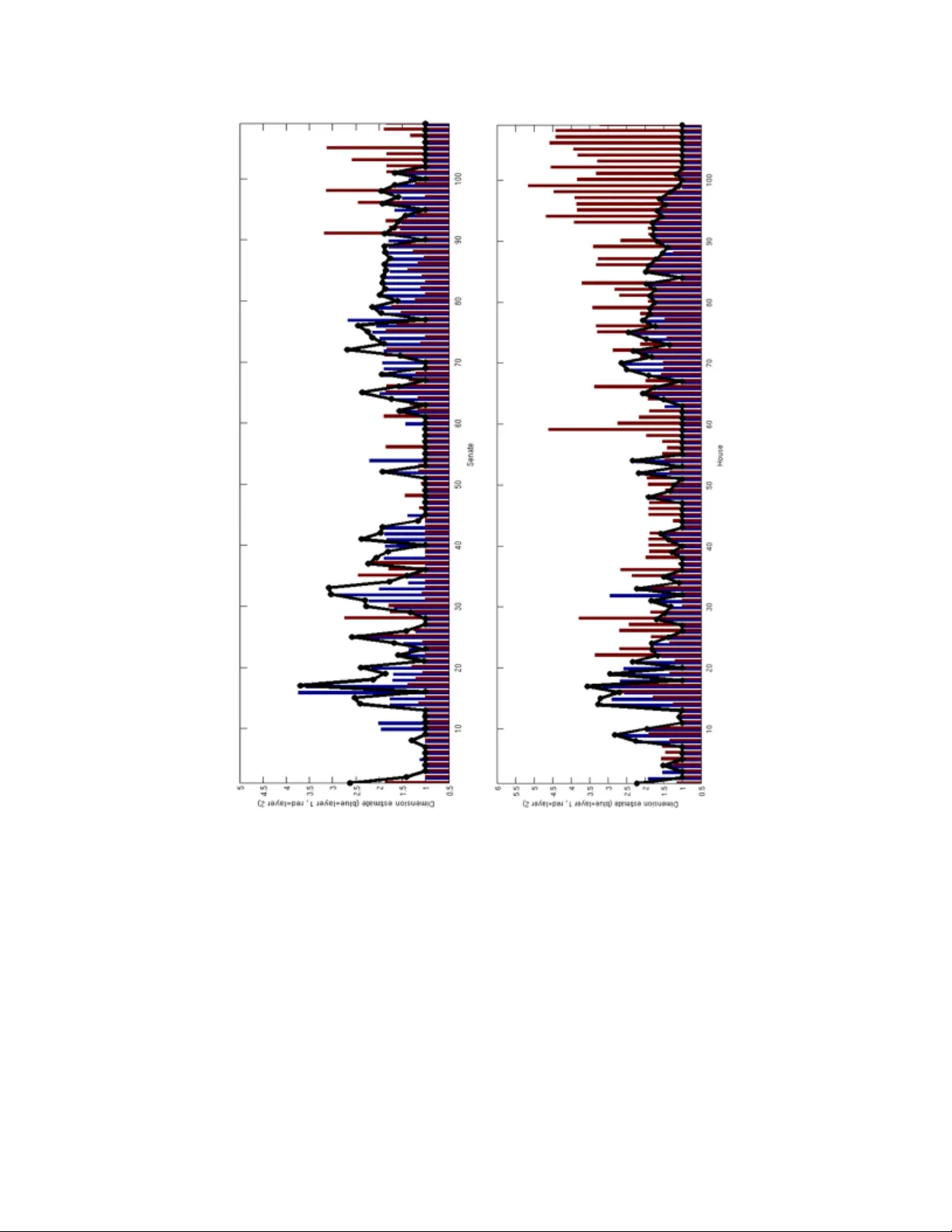
!" " Partition Decomposi tion for Roll Call Data G. Leibon 1,2 , S. Pauls 2 , D. N. Rockmo re 2, 3,4 , and R. Savell 5 Abstract In this paper we bring to bear so me new tools from statistical learning on the analy sis of roll call data. We pre sen t a ne w dat a - driven model fo r roll call voting that is g eometric in nature. W e construct the model by ada pti ng th e “Par tit ion Decoup lin g Metho d,” an unsuper vis ed le arni ng te chni que o rigi nal ly developed f or the analysis of families of time serie s, to produce a multiscale geometric description of a weight ed network associ ated to a set of roll call votes. Centra l to this approac h is the quantita tive noti on of a “motivation,” a cluste r - based and learned basis element that serves as a building block in the representation of roll ca ll d ata. Motivations enable the formulation of a q uantitative description of ideology and their data - dependent nature makes possible a quantitative analysis of the evolution of ideologica l factors. This appro ach is generally app licable to roll call data and w e apply it in particular to the historical roll call voting of the U.S. Hou se and Senate. This me thodolog y provides a mech anism for estimating the dimension of the underlying action space. We determine that the dominant factors form a low - ( o n e - o r t w o - ) d imensio nal representa tion with secon dary factors add ing higher - dimensional features. In this way our work supports and extends the findings of both Poole - Rosenthal and Heckma n - Snyder concerning the dimensionality of the action space. W e give a detailed ana lysis of several individual S enates and u se the Ada Boost tech nique from statistical learn ing to determ ine those vo tes with the most p owerfu l discrimin atory value . When used as a p redictive m odel, this g eometric view significantly outperforms spatial models s u c h a s t h e P o o l e - Rosenthal DW - NOMINATE model and the Heckman - Snyder 6 - fac tor model, b oth in raw accuracy as well as Aggrega te P roportional Reduced Error (APRE). """""""""""""""""""""""""""""" """""""""""""""""""""""""""""" " 1 Memen to, Inc., Bu rlington, M A, 0180 3 2 Departm ent of M athematics , Dartmou th College , Hanov er, NH 03 755 3 Departm ent of Co mpu ter S cience, Da rtmouth C ollege, H anover, N H 0375 5 4 The Santa Fe Institute, 1 399 H yde Park Road, Santa Fe, NM 8750 1 5 Thayer S chool of E ngineering , Dartmo uth Colleg e, Hanov er, NH 0 3755 " #" " Introduction Spatial models of parliamentary voting provide powerful geometric tools for th e analysis o f legislative bodies. Over the last three d e c a d e s , s p a t i a l m o d e l s h a v e b e e n d e v e l o p e d a n d substan tially refined. Important example s includ e the work of C a h o o n ( C a h o o n 1 9 7 5 ) , Cahoon, Hini ch and Ord eshook (Cahoon, et al., 1976), H inich and Poll ard (Hinich and Pollard 1981), Enelow a n d H i n i c h ( E n l o w a n d Hinic h 1984) , Hinich and Munger ( H i n i c h a n d M u n g e r 1 9 9 4 , 1 9 9 7 ) , O r d e s h o o k ( O r d e s h o o k 1 9 7 6 , 1986) , and Poole and Rosenthal (Poole and Rosenthal 1984, 1985, 2001, 2007 ). S patial m odels prod uce a low - dimensional representation of the (presumed) very high - dimensional “acti on space,” defined as the collection of “all contemporary political issues and government policies” (Ordesho ok 1976 , p. 3 08, as quoted in Poole 2005, p.14) that underlie the legisl ative process . These l o w - dimensional representati ons still hold an enormous am ount of information, as m easured by their ability to predict correctly the vast major ity of vot es c ast . The NOM INATE model s of Poole and Rosenthal are o f p a r t i c u l a r i n t e r e s t . Whe n app li ed to the dat a of the aggregated roll call votes over all Co ngresses, they produc e one - o r t w o - dimensional sp atial models that see m to expla in t h e m a j o r it y o f v ot i ng b e h a vi o r in th e U . S. C o n gr e s s ( Pool e and Rosenthal 2007) . In their words, “votin g is along ideological lines w hen positions are predictabl e across a wide set of issues ” (Poole and Rosenth al 2007, p . 3) . In th is con text “ ideolog y” h as a precise defin ition as their interpretation of the firs t dim ension (the m ajor dimension) of their s patial model, which is taken to be a measu re of the extent to which a legisl ator suppor ts gov ernme nt int erve ntio n in econo mic iss ues. The second dim ension is broadly interpreted in terms of region, but in fact, the detailed Poole - Rosenth al analysis sugges ts a m ore complica ted pic ture hid ing b eneath the surf ace. This is support ed by the $" " Heckman - Snyder work (H eckman an d Snyder 2003 ) in w hich a f a c t o r m o d e l i s u s e d t o s h o w t h a t a n interaction o f at least five spatial dim ensions is necessary to explain fully r oll call votes. As a whole, these models (and other s) show that the one - dimensional “liberal - conservative” axis of ideology, whic h app ears to captu re so much inform ation, is in fact a dyna mically changin g co mplex amalgam of a variety of factors. In this p a p e r , t h r o u g h a n e w f o r m o f a n a l y s i s o f r o l l c a l l v o t e s , w e introduce a new geometric model for parliamentary voting that articulates the complex structure of ideology, p roviding a quantitative and data - driven formulation that allows us to study the natu re and evolution of ideology as it is exp ressed in roll call votes. I n p a r t i c u l a r , w e a d a p t a new technique from statistical learning, the Partiti on Decoupli ng Method (P DM) (Leibon, et al. 2008 ) , to th e ana lysis of roll call data and apply it to historical r o l l c a l l v o t e s f r o m t h e U . S . C o n g r e s s . T h e P D M i s a v e r y g e n e r a l technique for th e ana lysis of correlatio ns in a fam ily of high - dimensional feature vectors. It was originally applied to the analysis of time series of stock prices. In that context the PD M art ic ul at ed t he mov eme nt o f stock prices as a linear combination of effects at variou s scales (e.g., market, sector, an d industry) and revealed b oth the overall contribution and interaction of these effe cts. The main point of this paper is to show t hat an a n a l o g o u s ( a n d i n f o r m a t i v e ) a r t i c u l a t i o n o f p o l i t i c a l s t r u c t u r e c a n b e a c c o m p l i s h e d b y adapting these methods for the analysis of roll call data. To adapt the PDM methodology to rol l call data, a legislator’s voting record is given a natural encoding as a point i n a high - dimensional space : a hist ory of an individual legisla tor’s m r o l l c a l l v o t e s ( e a c h encoded as either a 1, 0 , or - 1) is viewed as vector in a space of dimension m. T h i s e m b e d d i n g o f t h e voting records of a collection of legislators then si ts inside an m - dimensional “roll call space.” The distance between two legislat ors in roll call space is essentially a measure of the correlation of their roll call vote history. The identification of clusters in the data is the first step in constructing a data - driven definition of ideology and it provides a f i r s t f o r m o f d i m e n s i o n r e d u c t i o n : e a c h c l u s t e r g i v e s r i s e t o a cluster - averaged roll call vote, which suitably normalized defines a cluster - based “motivati on.” The m %" " votes of each legislator are then summarized by a vector of length N (where N is the n umbe r of cluste rs, in practice m uch sm aller than m ) co nsisting of the w eights m easurin g how close a leg islator’s v otes are to each of the cluster - averaged roll call votes. When we remove this dimensi on - reduced data from the roll call votes, we are left w ith a residual data series for each legislator. We can then repeat the clustering process on the residual s to reveal a new, subsidiary dimension reduction, which can in turn be removed from the new da ta. This proces s is iterated as long as the residu al data is distinguis hable from random data. The resul t is a model in which e very legi slator votes ac cording t o a set of wei ghted moti vations defined i n terms of the degree of a prio ri su pport (or the lack t h e r e o f ) f o r e ac h v o t e , a nd a l e g i sl a t o r’ s v ot i n g re c o r d is a w eighted sum of these motivation s. Aggregatin g all the weights with respect to a given collection of motiv ati ons in a clus ter of leg islators dete rmines a data driven notion of “ideology , ” effec tively defin ed as a collection of positions with high average weight. W e em phasize that these “ideological dimensions” are determined via unsupervised l e a r n i n g – t h a t i s , t h e n u m b e r a n d d e s c r i p t i o n o f t h e d i m e n s i o n s a r e determined by the data. This model has a number of satisfying features. First, it produces a quantifiable and m ore textured description of ideology, making possible the discovery of those issues and policy positi ons dictated by ideologica l conc erns. S econd, the data - driven description of id eology provides a means to quantify its evolution. Third, it creates a simple framework in which positions that might seem incongruous (at least according to some conventional labeling) can be p resent simultaneously within a single ideology. This is in a greement with the seminal work of Converse (Converse 1964) that showed that, in general, individual ideologica l constru cts are riddled with incons istencies and contrad ictions. N ote tha t this p oint of view is another feature that distinguishes our app roach from spatial mod els: a m ain underlying assumption in the construction of spatial models is that legislators maintain consistent ideologies, w hile our method does not require such an assumpti on and, indeed, may be used to evaluat e the validity of such a c laim. Fourth , &" " our model allows for the em ergence of m otivations for legislator s with different str engths – we i gh t s fo r a given motivation may be positive, negative, large, small, or even zero. This feature is absent from spatial model s, in whic h each l e gislator has an opinion positioned on each of the different axes (as indicated by their point in space) an d these op inions are c ounted e qually w hen com pared to a cut assoc iated to a v ote. W e use our approach t o a n a l y z e the roll call voting history o f the House a n d S e n a t e o f e a c h o f t h e U . S . Congres ses. 6 Th e f i r st l a y e r o f t h e re s u l t i ng m ul t i s c a l e v i e w c o n f ir ms t h e spatial m odel findings in that it exposes a dom inant effect of party identifi cation (see e.g., Poole and Rosenthal 2007). H o w e v e r , o u r PDM - insp ired ap proach provid es a more textured (yet still low - dimensional) description that goes beyond the one o r t w o d i m e n s i o n s o f t h e NOMINATE m o d e l o r t h e m u l t i d i m e n s i o n a l m o d e l s o f H e c k m a n a n d Snyder . Our a nalysis deco mpos es ea ch m ajor ideolog y into sub - ide ol ogies and the accompanying geometric analysis provides descriptive axes for each legislative body and coordinates for each legislator. Successive layers produce close r and closer approximati ons to the exact rol l call da ta and ult imately represent the data as a linear combination of ideological motivations for each legislator. From this we obtain predictive models for voting that we can compare to spatial models via correct classifica tion percentage and A PRE. In both cases, our methods significantly outper form both the N OMIN ATE model and the Heckman - Snyder 6 - factor model. Our exposit ion of the methodol ogy is aug mented by the pre sent ati on of det aile d PDM - based analyses of the 10 8 th , 88 th , and 77 th S e n a t e s . T h e s e e x a m p l e s p r o v i d e a g o o d d e m o n s t r a t i o n o f t h e variation in behaviors capable of being detected by the PDM . In the case of the 108 th S e n a t e , w e s e e t h a t t h e f i r s t layer is essentially one - dimensional and party - based while the second layer (appearing on a finer scale) reflects a new pa rtition of the legislato rs d istinct from the party - based partition of the first layer. In the 77 th a n d 8 8 th S e n a t e s t h e i n i t i a l l a y e r o f c l u s t e r s ( a n d h e n c e t h e l e g i s l a t o r s ) c a n n o t b e a r r a n g e d a l o n g a """""""""""""""""""""""""""""" """""""""""""""""""""""""""""" " ' "()"*+) , "-. ) ", / -/ "/ 0 /12/ 3 2) "/ -"4 ) 1-. "5 6 6 2) 7+ " “V oteview Website”, http:/ /www.voteview.com 8" '" " single dimension. I n t h e 8 8 th S e n a t e , w e a g a i n f i n d a s e c o n d l a y e r d ominated by issue - based concerns rather than party , while in the 7 7 th the residual data exhibits no additional detectable structure. Our iss ue - based characterization of the second layer of the 108 th a n d 8 8 th S e n a t e s i s s i mi l a r t o t he f a c t o r s i d e n t i f i e d b y Poole - Rosenthal (Poole and R osenthal 200 7) as aspects of the second dimension of their spatial model. Our analysi s diffe rs from spatia l models in that our explanat ion of the second layer uses a complete ly different geometric model. In a second novel use o f s t a t i s t i c al l e a r n i n g w e i d e n t i f y t h e “ b e s t ” s e p a r a t i n g issues via the statistic al approa ch of A daBo ost (Freu nd and S chapire 199 7, 1999) . T his yield s a qualitative descript ion of issues that split the larger party ideologies into partially conflicting s ub - ideologies . O ur procedure also giv es us a quantitative compariso n b etween the tw o la yers, allowing us to measu re their re lat ive stre ngth . In con tra st, th e methods used to unders tand th e dimensi ons produc ed in spatial m odels are based o n necessarily sub j ective classifications of roll call votes (see e.g., Poole and Rosenth al 20 07 ). In summary, our a p p r o a c h a n d t h e t o o l s w e u s e a r e n o v e l i n t h r e e w a y s . F i r s t , w e u s e u n s u p e r v i s e d metho ds to l ocat e ge ometr ica lly si gnif ica nt clust ers in the n etwor k a ssoc iat e d to the roll call data . Second, the i t e r a t i v e m e t h o d o f r e m o v i n g a n d r e e x a m i n i n g t h e r e s i d u a l d a t a f o r a d d i t i o n a l s t r u c t u r e i s entirely new. Third, our use of the A daBoost algorithm to help describe qualitatively the motivations is novel in this context a n d i s q u a n t i t a t i v e . W e e x p e c t t h i s a p p r o a c h t o b e o f g r e a t u s e i n f u t u r e a n a l y s e s o f roll call data, either independe ntly or as a compan ion to spatial mode ls. Spatial models We bri efl y re vie w some aspec ts of the spat ial mode ls in the literature: th e mod els of Poole and Rosenthal (Poole and Rosenthal 2 007) , the Bay esian e stimatio n of ideal po ints of Clinto n, Jack man and Rivers (Clinton, et al. 2004 ) , and the line ar proba bility mo del of He ckma n and Sn yder ( H e c k m a n a n d S n y d e r 2004) . 9" " Conside r the simplest o n e - dimensional spatial m odel in the context of a simple example of a single bill voted on by a collection of legislators. In this case, each bill and vote is assigned an ideal point o n t h e real line. The line is m eant to encod e the position o f the bill relative to som e chara cteristic. For each bill a legislator exam ines its ideal point with respect to her own position on the b ill relative to that ideal point: if the vote p o s i t i o n i s t o t h e l e f t o f t h e b i l l , s h e v o t e s “ y e s ” a n d i f t o t h e r i g h t , s h e v o t e s “ n o . ” H i g h e r - dimensional models are constructed analogously: bills are assigned an ideal hyperplane in n - dim ensional Euclidea n space. Votes are cast accordin g to the spatial relat ionshi p of the ideal points and the bill: a legislator w ill vote “ye s” if to on e side of the hyperplane and “no” if to the other. In th eir work over the last two decades, P o o l e a n d R o s e n t h a l have show n t h a t t h e p a r s i m o n i o u s m o d e l described above holds great power. If the ideal positions are calculated using a maximum likelihood estimator from the roll call d ata, the resulting voting model correctly predicts over 80% of all vo tes in the history of the U.S. Congress. Moreover, they find, with the exception of two periods in history, that a one - o r t w o - d i m e n s i o n a l m o d e l i s s u f f icient to explain the vast major ity of votes. Poole, Ros enthal and their co - authors have refined these ideas over the last three decades, producing the family of NOMINATE scoring systems based on these spatial models (cf., Poole and R osenthal 1984, 1985, 2007; McCarty, et al. 1997, 2006; Poole 2005). Clint on, Jackman and River s ( C l i n t o n , e t a l . 2 0 0 4 ) e s t a b l i s h a B a y e s i a n a p p r o a c h f o r e v a l u a t i n g legislative preferences from roll call data in the context of one or mo re m odels of legislative beh avior. Th eir framework is broadly applicable an d can be adapted easily to focus o n is s u e s of sp e c i fi c i n t e re st o r to inco rporate addition al asp ects or assumptions. As an application , their m ethods can be used to estimate ideal points for spatial models of voting . Their work allow s fo r a m uch mo re refin ed (a nd f aster) probabilisti c estimation of ideal points with very few restrictions on the underlying data. Moreover, their technique s, unlike th ose of P oole - Rosenth al, allow for an accurat e analysis of er ror in t he ideal point estimations. :" " Heckman and Snyder (H eckman and Snyder 2003) p r e s e n t a n o t h e r a p p r o a c h . T h e y c o n s t r u c t a l i n e a r probability model to which a factor analysis is applied. Their results show that roll call voting is not determined by just one or t wo dimensio ns, but often many more ( u s u al l y a t l e a s t f i ve ) , indica ting a m ore complex structure. The H eckman - Snyder model has a computat ional advantage – i t i s l i n e a r a n d h e n c e computationally inexpensive. Its output is the collection of significant eige ndata 7 a s s o c i a t e d t o a similarity m atrix derived from the roll call da ta. If, a priori, the nu mber of sign ificant eige nvectors is fixed and they are used as coordin ates of ideal p oints in a E uclidean space, they recover a close ana logue 8 of the Poole - Ros e nthal spat ial model. The Partition Decoupling Method ( PDM) Key to our meth odolo gy is an adapt ati on of the Par tit ion Decoupl ing Method (PDM) of Leibon, et al. (Leibon, et al. 2008). Alth ough originally developed for the analysis of a collecti on of time ser ies data, the PD M provide s a general approa ch to the analysis and articulation of multiscale chara cteristics in high - dimensional data. In particular, the PDM pro duces a multisca le (i.e., hierarchical) model for roll call voting. We explicitly point out th at the resulting model is not a spati al model in the sense described above. For a given legi slati ve body (e.g., U.S. Senate or House of Representative s) over a fixed timeframe let d e n ot e t h e v o ti n g r e co rd of l e g i s l a to r i ( i = 1 , … , n ) . It will be a v ec to r o f l en gt h m , where m i s t he number of votes in that session. The j th e n t r y o f r e c o r d s t h e v o t e o f l e g i sl a t o r i o n b i ll j . It is equal """""""""""""""""""""""""""""" """""""""""""""""""""""""""""" " 9 ";<1=)>, /- / ? "@) A) @+ "-6 "- . ) ")1= ) > 0 / 2* )+ "/ > , ") 1= ) > 0) B -6 @ +"6 A"- . ) "C /-@1D8" " : "E.1+"1+"F/@ -1B * 2/ @2G "B2) / @"1A"H )"@)B/22"/ "- . ) 6 @) -1B / 2"@) + * 2-"6 A"5 6 6 2) "I5 6 6 2) "# J J& K "H . 6 "+ . 6 H +"-./-"1A"0 6 -1> = "1+"F )@A)B-" I/B B6@,1>="-6"-.)"+F/-1/2"C6,)2K"-.)>"-.)"A1@+-">6>-@101/2")1=)>0)B-6@"6A"-.)",6*32) L B)>-)@),"@622"B/22"C/-@1D"1+" )D/B-2G"-.)"1,)/2" F61>-"0/2*)+"A6@"-.)"6>) L ,1C)>+16>/2 "+F/-1/2" C6,)28""E.)")1 =)>,/-/"6A"-.)" ,6*32) L B)>-)@),"C/-@1D" 1+")++)>-1/22G"H ./-"M) BN C / > "/ > ,"O>G,)@"*+)"1>"-.)1@" />/2G+1+8" "" " P" " to 1 o r - 1 , de pendin g on w hether leg islator i v o te d “ y ea ” o r “n a y ,” and it is 0 i n th e c a se t h a t l e g i s l a t o r i either was not present, did not vote, or voted “present” on the j th bi ll . Th e roll call matrix, V, is the n x m array of votes. To use only releva nt data, we remove all v o t e s w i t h a m i n o r i t y o f l e s s t h a n 2 . 5 % of the total body 9 . Our mod el represent s each legislator’s roll call record as a weighted sum of basic “motivations” , . (1.1 ) A motivat ion, , is a unit ve ctor of len gth m. The entries of the motivation e n c o d e t h e s t r e n g t h o f su pport (or opposition in the case of a negative weight) associated to each of the individual votes. In this way the motivat ion vector is the record of an ideal voter with respe ct to the issues underlyi ng the motiv ati on. F o r e xa m p le , i f i s p o s i t i ve a n d la r g e , w e inter pret this as in dicating that the ideal voter associated with the motivation would v ote “ yes” on the k th vote . Similarl y , if is larg e and negati ve , -.)" B6 @@)+ F6 >, 1>= i d e a l v o t e r w o u l d v o t e “ no” on t he k th v o t e . The weights t h e n r e p r e s e n t t h e individual weights for legislator i t h a t r e f l e c t h o w t i e d e a c h l e g i s l a t o r i s t o a g i v e n m o t i v a t i o n , i.e., how closely a legislat or’s true voting matches t he ideal voting encoded in the motivat ion vector . The flexibili ty in choice and number N of the m otivations (all we require is unit length and the ability to represent the roll call data) is at th e heart of a m o r e s u b t l e d e f i n i t i o n o f i d e o l o g y t h a n a b l a c k a n d w h i t e yea - nay d ecision on a given vote. Motivations can either be declared a priori or d iscovered from the geometry of the roll call space via clustering. We pu rs ue t h e l a t t e r a p p r o a c h , e x t r a c t i n g p l a u s i b l e candidates for the motivations (and the corresponding w eights) acco rding to where the majority of the """""""""""""""""""""""""""""" """""""""""""""""""""""""""""" " P "()"B.6 6 +) "- . 1+"- . @) + . 6 2, "-6 "C /N)"6* @ "/ > /2G + 1+"B 6 C F/@/3 2) "-6 "-. / - "6 A"5 6 6 2) "/ > , "Q 6 +) > - . /2"I 5 6 6 2)"/ > , "Q 6 + ) > -. / 2" #JJ9K8 " !J " " informatio n in the data lies. Fort this, the basic obj ect of study is th e n x n co rrelation m atrix , 10 S determined by the roll cal l matrix. The entr ies i n S are defined by . (2.1 ) Note that the corr elat ion betwe en l egis lato rs i and j is simply the c osine of the ang le between the center ed legislator vote vectors in m - dimensional space and is easily relat ed to the distance between the points defining the legi slators in the m - dimensional roll call spa ce. The matrix S al so can be thought of as defining a weighted network o f l e g i s l a t o r s i n w h i c h t h e s t r e n g t h o f c o n n e c t i o n b e t w e e n a n y t w o legislators is g iven by th e correlatio n of their ro ll call vectors . From this geometri c embedding o f t h e l e g i s l a t o r s w e d e r i v e t h e m o t i v a t i o n s v i a a p a r t i t i o n i n g o f t h e legislators into ge ometrica lly determin ed clusters. Each cluster determine s a motivation given by the normalized mean (centr oid) of the clust er. Genera lly , these motivat ions will be li nearl y independent. The first “layer” in the roll call data is then given by its p r o j e c t i o n o n t o t h e s e m o t i v a t i o n s . T h e r e s i d u a l relative to these motivation s is obtained by subtracting this first projection. The process of clustering, constructing motivat ions, and projectin g, and finally , compu ting residua ls, can now be repeated until the residual is indistinguishab le from noise. We’l l now be more preci se: let k 0 d e n o t e th e n u mb e r o f cl u s te r s fo u n d in t he o r i gi n a l n o r ma l i ze d r o ll c al l data. For each clust er we create an average voting profile by taking the (normalized) mean of all votes over the m embers of the cluster. Let denote these fir st scale (or level) motivations. T o calculate the w eights w e project the vote vector o f t h e i th l e g i s l a t o r o n t o t h e s u b s p a c e """""""""""""""""""""""""""""" """""""""""""""""""""""""""""" " !J "E.)@)"/@) "C />G",1A A) @) > -"B . 6 1B )+ "6 A"+ 1C 12/@1-G"6> ) "B/ > "* + ) "/ -"-. 1+ "+ -/ = ) "I) 8= 8"F ) @B ) > -/ = ) "6 A"0 6 -) +"1> "B6 C C6> K8"" ()"F) @A6@ C)," 6*@" />/2 G+)+ "H1- ."/" B6CC6> "06- )"+ 1C12 /@1 -G" /+"H) 22" />," A6*> ,"+1 C12/ @"@ )+*2 -+8 " !! " " spanned by . The weig hts a r e t h e c o e f f i c i e n t s o f t h e p r o j e c t e d v e c t o r w r i t t e n in term s of the motivations . 11 From this we derive a first “scale” approxi mation to the roll call space, given by This accomplishes an initia l di mension reduction from m ( t h e n u m b e r o f v o t e s ) t o k 0 , the numb er of clusters in the f irst scale . W e can rep eat the abo ve proced ure on t h e re s i du a l to uncov er an additional l ayer of structure. That i s, we can clust er the residual time series and compute the corresponding motivations defined as the means of the new clusters. We can iterate this process and each additional layer gives a next term in what becomes a better and better approximation to the original d ata. If we have L layers w ith mo tivations a n d c o e f f i c i e n t s , (where l = 1,… ,L a n d k 0 ( l ) d e n o t e s t h e n u m b e r o f c l u s t e r s f o u n d a t s c a l e o r l e v e l l ) then at ea ch scale we acqu ire an additional level of app roxima tion given by We rep eat thi s pr oce dur e unt il the co rr ela ti on st ruc ture of the residual data , , i s i n d i s t i n g u i s h a b l e f r o m t h e c o r r e l a t i o n s t r u c t u r e o f a r a n d o m l y """""""""""""""""""""""""""""" """""""""""""""""""""""""""""" " !! "RA"-.)" "/@)">6-"21> ) /@ 2G "1> , )F ) > , ) > - S"-. 1+ "* +* / 22G "+ 1=> 1A 1)+ "/ "F 6 6 @"B . 6 1B ) "6 A"-. ) "F / @/ C )-)@+8""R> "+ * B . "/"B / + )S" H)"H6*2, "+1CF2 G"/,T*+-"-.)"F/@/C)-)@+8 " !# " " reordered version of the residu al data. This give s a “multiscale” or “hierarchical” appro ximation to the roll call data as " " When app lie d t o th e Hou se and Senat e, in a numbe r of cas es (the 3 rd , 4 th , 5 th , 6 th , 7 th , 9 th , 10 th , 11 th , 23 rd , 57 th , 58 th , an d 77 th S e n a t e s a n d t h e 2 nd , 3 rd , 18 th , 31 st , 37 th , a n d 4 4 th H o u s e s ) a s e c o n d l a y e r c a n n o t b e computed as there are no demonstrably significant clusters. In other C o n g r e s s e s , w e c a n c o n t i n u e t o uncover several more layers of informati on by this test. In what follows , w e c h o o s e t h r e e e x a m p l e s a n d discuss the information obt ained by invest igating one a dditional l ayer. At e a c h s c a l e , t h e p r o j e c t i o n s o n t o t h e m o t i v a t i o n s a c c o m p l i s h s o m e f o r m o f d i m e n s i o n r e d u c t i o n ( w i t h dimension generally equal to the number of clusters) of the original data. As a further refinement, these lower - dimensional approximations can be a n a l y z e d i n a n d o f t h e m s e l v e s , f o r e x a m p l e , v i a multi dime nsio nal s caling ( MDS – see B org and G roenen 2005). Further analysis of the motivations is accomplished via the use of the AdaBoost algorithm (Freund an d S chapire 1997). In general, AdaBoost identifies which p ortions of a d ata stream best distinguish among a list of clusters. In our case, we can use AdaB oost to identif y ro l l c a l l v o t es whi ch b es t determine t h e b ou n d a r i e s of th e cl us t e r s o f l e gi sl a t or s. We inter pr et the iss ues beh in d these vot es as the i ssues that best separate (and hence help define) the motiv ati ons asso ciat ed to the clus ter s. It is c lear that clustering is a key step in the pro cess. Th is can be a ccomplished in many ways, but following the PDM me thodology, we choose to use a form o f spectral clustering . Gene rally speak ing, spectral clustering refers to the determination of clusters in high - dimensional or network data via some use of the ei gendata of the graph Laplacian (see the Appendix A) , a matrix related to the similarity matri x (e.g., distance matrix, in the case of geometric data or the adjacenc y ma trix in th e case of a netw ork) of the d ata. We use the eige ndata to dete rmine two parameters: the nu mber of clu sters, , an d l , a “ n at ur a l ’ !$ " " dimension f o r e mbeddi ng the data netwo rk . After dete rminin g k 0 w e t h e n e m b e d t h e n e t w o r k i n l dimensions and use the k - means al gori thm ( see e.g., Du da et al ., 2000) to fin d th e bes t k 0 clusters. For both of these parameters th e second eigen vector (i.e., the eige nvector c orresponding to the second smallest eigenv alue) of the graph Laplacian 12 will provi de the key i nforma tion . T his is the so - called Fiedler vector, wh ic h w e d e n o t e a s . The Fiedler ve ctor is know n to encode the coarse globa l geom etry of the network (see, e.g., Chung 1997). As has been shown in a variety of differ ent settings, the Fiedler vector is effectively the solution to a soft version of various formulations of the problem of finding the optimal decomposition (e.g. , m inimum cut) of a network into two components (Luxburg 2007, Ng, et al. 2004). The Fiedler vector is indexed by the data or network elements and the clusters can be determined by optimally clustering the entries in the Fiedler vector (see e.g., Luxburg 2007) to determine the best decomposition. We use a varia ti on in whic h the numbe r of valu es aro und whi ch the Fie dle r vect or val ues are clus ter ed is an estimate for the number of clusters. To compute this number we fit the distribution of values in by a Gaussi an mixtu re dist ribut ion wit h the number of compone nts rang ing from 2 to 20. We the n use the Akaike informati on crite rion (AIC) 13 (Akaike 1974) , to me asure the clo seness of fit. In the case where the minimum AIC value is at least 5% smalle r than its nearest competitor, we tak e the number of components in the fitted distribution w ith minimum AIC as our choice for . If there are multiple AIC values within 5% of the minimum, we take the median value of the num ber o f compo nents of those fitted distributi ons as . T his last step is some what arbitrary, but it prevents drastic c hange s in the num ber of clusters unless tr uly warranted. """""""""""""""""""""""""""""" """""""""""""""""""""""""""""" " !# "E.)"U/F2/ B 1/ > "1+"+ G C C )-@1B"F6 + 1-10 ) "+ )C 1,)A1>1- )"/ > , "A6 @"-.)+)"@ 6 22"B/ 22") D / C F 2)+S"./+"J "/ +"/ > ") 1= ) > 0/ 2* ) "H 1-." C*2-1 F21B 1-G" 6>)8 " !$ "()"/2+6 "* +) , "/ > 6 -. )@"+-/>, / @ , "B@ 1-) @16 > S"-.)"V/G ) +"1> A6@C/ -16 > "B @1- )@ 16 > S"G 1)2, 1> = "+ 1C 12/@"@)+* 2-+ 8""E. ) ">* C 3 ) @"6A " )+-1C/-),"B2*+-)@+"H/+S"1 >"=)>)@/2S"+21=.-2G "26H)@"-./>"H.)>"*+1>="-.)"WRX8" " " !% " " After determi ning the number of clust ers to fin d in the d ata, the next step is to pick a dimension for embedding the data. This will be the environment that we use to look for the clusters. This i nitial dimension reduction is our estimate of l, the appro priate dimen sion for the data. It is d etermine d via an esti mate of the number of sign ifi cant eig envec tors in the grap h Lap laci an. Here, “s igni fic ant” means tho se eigenvectors w ith nonzero eigenvalues that are smaller than w ould be expected from a suitable null model . Thi s in t urn means that the se non zero eige nval u es are less than a worst case estimate of the eigenvalue for a Fiedler vector of reasonable null model for t his data. This builds on the fact that the s mall eigenvalues and corresponding eigenvectors for the graph Laplacian (like the Fiedler vector) encode t h e basic clustering information for the network or data (see e.g., Luxburg 2007 for a nice discussion of this). The null model i s given by rando mized roll call data constructed by r andomizing the votes of th e legislators for ea ch vote. In other w ords, f or a specific vote, we record the number of yes and no votes and then, for the randomized version of that vote, assign these yes and no vo tes randomly among the legislators. Executing this over many votes destroys any structure or affinity between groups of legislators. More preci sel y, for each set of roll call data , we crea ted 25 randomiz ed versions of the roll call data and computed the Fiedler value for each one. W e choose t o b e t h e n u m b e r o f n o n z e r o e i g e n v a l u e s o f t h e Lap lacian associated to the ro ll call da ta that are less than the minimum of all Fiedler values for the simulated roll calls. This procedu re en sures that the information encoded in the eigenvectors a nd eigenvalues that we use is distinguishable from “informat ion” that may h ave arisen due to ch ance. We emp has ize tha t t his fi xed meth od of par ame ter se lec ti on i s a us e of uns upe rvi se d le arn ing – we d o n ot finesse our choices of p arameter or method for individual instances or u sing additional information. We do th is for tw o reasons. First, we wish to make the method as transparent as possible. Second, we view this metho d as possib ly a first step, su bject to refin ement in individual c ases as wa rranted. T hat is, this initial estim ate of dimen sionality then can be a n a l y z e d f u r t h e r ( e . g . , v i a m u l t i d i m e n s i o n a l s c a l i n g ) i n !& " " order to achieve a better understanding of the structure in the reduction. This is accomplished in some of our examples. Later on, we will indicate where the results may be pointing towards a refine men t in parameter choice and/or method. We n ow sum mari ze t he met hod us ed in t he ex ampl es be low : 1) Compute the c orrel ation matri x S from the d ata, . 2) Form the gr aph Laplaci an and f ind it s eigenval ues and eigenvector s. 3) Deter mine k 0 , the nu mber o f cluster s, via an A IC - based analysis of t he Fielder vect or. 4) Deter mine l , the n umb er of sig nificant eigen vectors of the graph Laplacian via co mpar ison with random m odels. 5) Embed the roll call data in l - dimensional E uclidean space via the coord inates g iven by the first l eigenvectors of the graph Laplacian. Use k - means to find k 0 c l u s t e r s . D e t e r m i n e t h e m o t i v at i on s as the mean votes of all members of each cluster. 6) Project the data onto t he subspace determine d by the motivati ons, for ming . 7) Find the residual data 8) If the residual is not in distinguishable from rando m n oise, rep eat step s 1 — 7 to form the next layer, otherwise stop. Remarks: 1. Whil e we cho ose to do a t m ost t wo ite ra ti ons of t he procedure, it can be iterated until the stopping condition in Step 8 i s met. !' " " 2. As we will see below, it is useful to apply multidi mensi onal scali ng after determi ning the clust ers to get a bette r idea of the true dime nsionality of the first (o r dependin g on the iteration , l th ) layer. 3. Upon project ing the dat a ont o the moti vati ons, AdaBoos t can be (and is ) used to determi ne the votes that best disti nguish the cl usters. In the next section we see the process in action. Examples In this section w e ex plore t h r ee examples, the 1 08 th , 88 th , an d 77 th S e n a t e s . To provide fu rther intuition for our m ethodology we begin with a m ore detailed analys is of the Fied ler vector. Recall th at the num ber of clusters in the entries in the Fiedler vector will serve as our estima te of the n umbe r of clu sters in the data. This approach is motivated by various analytic and geometric properties of the eigenvector. W e try to provid e a mo re intuitive rationale by showin g how this sim ple piece of spec tral inform ation ac tually encodes a g reat d eal of e xplanatory power for the roll c all data. W e then continue on to give the full analysis for these dat a sets. The Roll Call Fie dler Vecto r. A l t h o u g h i t n e e d n o t b e t r u e g e n e r a l l y f o r a n e t w o r k , i t t u r n s o u t t h a t i n the case of roll call data, the Fieldler vector i s h i g h l y l o c a l i z e d – m o s t o f i t s v a l u e s a r e c o n c e n t r a t e d near a small list of values. In the Congressional roll call data often the values of ( i n d e x e d b y t h e legislators) a re conc entrated around two values, one negative and one positive. Thus, for most Congres ses just u sing the sign o f the entries of s o r t s t h e l e g i s l a t o r s i n t o t w o g r o u p s . T h i s g e n e r a l l y recovers the b a s i c p a r t y s p l i t r e v e a l e d b y t h e NOM INATE models, but other mo re interesting divisions can also occur. In Figure 1, we display th e results for the 1 08 th , 88 th , and 77 th S e n a t e s . In each grap h the entries of a r e plotted against the senator indices . These have been listed so that the first block is composed o f a l l t h e !9 " " Democra ts, t he next is al l t he Republicans, and finally there are the Independents (if any). W e now discuss these examples in s ome detail. (INSERT FIGUR E 1 HER E) Example 1 – t h e 1 08 th S e n at e . Here t h e v al u e s ar e t i gh t l y cl us t e r ed ar o u n d 0 .1 an d - 0.1 and proximity to these valu es essentia lly distin guishes the two parties. The most “ ou t o f p l ac e ” me m b er is Se n . Mi ll e r ( D - GA) whose co ordi nates ( 11, - 0.08474), are marked with a square containi ng an “x. ” S e n . M i l l e r i s a Democra t who often broke with his party to suppor t the Republi can posit ion and who attended and spoke at the 2004 Republican National Convention, endorsing President G. W. B ush for re - election. There are several other membe rs (m arked b y filled squares) who differ signi fic antl y from their close st clust er. Among t he Democ rats are Senat ors Baucus , Bre aux, Linco ln, and B. Nels on. Among t he Rep ubli cans are Senators Chaffee, Colli ns, Snowe, and Spector . T h e s e s e n a t o r s a r e k n o w n t o b r e a k w i th their p arty on certain issues. Example 2 – t h e 77 th S e n a t e . The picture here is much less clear – t h e D e m o c r a t s m o s t l y h a v e positive values w hile the Republicans mostly have nega tive values. Howe ver, there are a signific ant numb er of member s of bo th parties with v alues very close to ze ro. There are t wenty - two s e n a t or s , ma rked by filled black squares, wit h values betwee n - 0.05 and 0.05. Mo reo ver , s eve n De mocr at s ( eac h ma rke d b y a n “x ”), Senators Adams, B ulow, D. Clark, J. Clark, McCarren, W alsh an d Wheeler, lie within the cluster defined by the negative values of the Fiedler vector that is generally associated with the Republican senators. All of these senat ors broke with t he Democratic party on various important issues, indica ting a closer ideolo gical alignment with t he Republican Part y than general ly evidenced by a Democrat. Example 3 – the 88 th Sen at e. Her e w e ha ve a r at her di ff er en t pi ct ur e. Th e l ast gr ap h i n Fi gu re 1 sh ows th e Fiedler vector data for the 88 th S e n a t e w i t h D e m o c r a t s l i s t e d f i r st, followed b y Republicans w ith color annotation by region (red = midwest, blue = northeast, green = south, black = sou thwest, yellow = west). !: " " We se e De mocr at s sp li t in to two bas ic group s of dif fe ren t signs and Repu bl ica ns, whi le hav ing mos tly negative va lues, also have a num ber of m emb ers with positive v alues. W e see that in th is case, o ne aspe ct of the Fiedler vector is associated w ith region. This is not surprising as one of the signature pieces of legislation in the 88 th Congress w as the Civil Rig hts Act of 19 64 for which voting split by reg ional as well as party lines. This initial investigati on of the 108 th , 88 th , and 77 th S e n a t e s g i v e s e v i d e n c e f o r o u r c l a i m t h a t t h e F i e d l e r vector provides a coarse classi fication of the Congress in questi on. O ur interpretation of the analysis of the examp les is th at the Fiedler vec tor captures party lo yalty. In Appen dix B, we pre sent simulatio ns that support the claim that the Fiedler vector provides a useful simple classification tool for roll call data. Th e Full PDM Analysis. The analysis of the Fiedler vect or and its classif icati on strength provides one view of t he question of dimensionality of the representation which f its well with the results of the NOMINATE models, echoing the finding of one or two dom inant dim ensions for most of th e U .S. Congres ses. However, the Fiedl er vector is just the firs t piece of our multidime nsiona l PDM - based analysis. As we outli ned above, a more detaile d ana lysi s of the Fiedler vect or provide s the est imat e of , t h e appropriate num ber of clusters in the data, wh ich are then actually determined in l - dimensional space, for a choice of l a l s o g u i d e d b y t h e r o l l c a l l F i e d l e r v e c t o r . I n s o d o i n g w e a r r i v e a t a n i n i t i a l d i m e n s i o n reduction, giving an app roximation of th e orig inally m - dimensional roll call data (where m i s t h e nu mb e r of votes) as - dimensional data determined by the projection onto the space spanned by the motivations. This pr ocess is the n repea ted on each s ucce ssive residual. The initi al dimension reduction given by the number of cluster s ignores the relationshi ps between the clusters. For example, it could be that all the clusters effectively collect on a single line in l - dimensional space. We can use multidim ensional scaling to provide an estimate of the aggregate dim ension of the !P " " approximation that takes into accoun t these interrelationships. To do this for the first layer, we compute the m atrix of pairw ise Eu clidean distances between the we ighted sums o f t he motivations for legislators by calculating t he length 14 o f t h e d i f f e r e n c e b e t w e e n t h e a p p r o x i m a t i o n v e c t o r s : . We then comp ute th e mu ltidimen sional scaling of th is dissim ilarity matrix for dimensions one through ten and the str ess of each representation. The estimate of the dimension is then the interpo lated dim ension b etween one an d ten w here the stress reaches 0 .1. This is a com monly used cutoff po int for this method (see e.g. Borg and Gronen, 2005). We repeat the analysis f or the second layer (fo und in the residual as determin ed by removing the first laye r), using , as well as for the combination of the first and second layer, where . Figure 2 pr esents t he result s of doi ng this MDS analysis on t he first t wo layers for all U.S. Congresses. As indicated, the height of the blue b ar is the dimen sion of the first layer, the height of the r ed bar is the dimension of the second layer and the black curve gives the dimension of t h e m o d e l p r o d u c e d b y combining the two layers. Th e b lack curve further gives an indication of the relative strengths of the two layers and the interactio n betwe en them . (INSERT FIGUR E 2) Our resul ts suppo rt the bas ic resul ts obta ined by the NOMINATE models – t h e f i r s t l a y e r i s m o s t o f t e n one - dimensional with notable exceptions such as the period encompassing the 72 nd t h r o u g h 9 0 th S e n a t e s . However , in t he sec ond lay er, we see a more compli cat ed pict ure wi th many Houses a nd Senat es sh owing high - dimensional second layers, particul arly in periods which precede a jump in the dimension of the first layer or as th e dimen sion of the first layer retu rns to one . """""""""""""""""""""""""""""" """""""""""""""""""""""""""""" " !% "E.)"2)>= -. "/ "0 )B -6 @ " "1>"<*B21,)/> "+ F /B ) "1+ "=10 ) > "3 G " 8" " #J " " Our combi nati on of es timat es (t he bla ck curv e) prov ides a potent ial expla nati on of th e diff erenc e be tween the NO MIN ATE and Heckm an - Snyder models. Like the Heckman - Snyder factor analy sis, we too find many fact ors /dime nsio ns that c ontr ibu te to an expla nati on of the roll call data, but our factors a re naturally related to one another in a manner that often p r o d u c e s d i m e n s i o n a l e s t i m a t e s i n l i n e w i t h t h e NOMINATE model . This refl ects the measurement of sca le inherent in our methods – t h e f i r s t l a y e r motiv ati ons occur at a coar ser scale than those of th e second layer and, by the eviden ce shown in Figure 2, dominate the explanation of most roll call votes. However, the extra dimensions stil l provide valuable informatio n, cre ating a high - dimensional “fuzziness” around the low - dimensional approximation, a result that helps ex plain the n ecessity o f the larger n um ber of dimensions in t he Heckman - Snyder fact or models. Carryi ng through the examples given above, we now give a com plete PDM - based analysi s of the 108 th , 88 th , and 77 th S e n a t e s . T h e 77 th Congress g r a p p le d with th e entry o f The U nited Sta tes into W o r l d W ar II . The hallm ark le gislation of th e 88 th C o n g r e s s w a s t h e C i v i l R i g h t s A c t o f 1 9 6 4 , f i l i b u s t e r e d f o r o v e r 14 hours by Sen. Byrd, and splitting the Dem ocratic Senators along regional lines. The 108 th Co n g r e s s i s considered one o f the m ost politically p olarized Congresses since Reconstruction (McCary, et al. 2006 ) , with the vast maj orit y of vot es p redi cted accu rate ly b y id eolog ical ide nti fica tion alo ne. Example 1 – the 108 th Sen ate : Poole and Ro senthal find that the 108 th Sen ate is wel l - described by a si ngl e dimension that captures party ideology. Our methods reveal two significant layers and thus, more than one dimension’s wort h of informati on. The information in our first layer is cons istent with the picture painted by the one - dimensional summary of Poole and Rosenthal, but provides both quantitative and qualitati ve descriptions of the contributing ideologica l fac tors. T he second layer pro vides a new le ns th rough which we can see org anization of the Senate t hat is issue - based ( rather than based on part y identific ation). #! " " At the fi rst scale the Fiedler vect or split s the 108 th S e n a t e i n t o s e v e n c l u s t e r s . One of the “Republ ican” clusters contains a single Democrat (Sen. M iller) but otherwise the clusters are uniform in party: t hree are Republi can ( including the barely “m ixed” c l u s t e r c o n t a i n i n g M i l l e r ) and four a r e D e m o c r a t s . U s i n g t h e v a l u e s a s w e i g h t s o n t h e m e a n v o t e v e c t o r s o f t h e c l u s t e r s ( m o t i v a t i o n s ) r e d u c e s t h e r o l l c a l l v o t e s of thi s S enate to a combination of s even f a c t o r s . A r e d u c t i o n o f t h i s t o t w o d i m e n s i o n s v i a multi dime nsio nal scaling produces a stress equal to 0.0171 , imp lying that dista nces in this reduction ar e relatively true. A two - dimensional view has the furth er adv antage of enab ling a visualizatio n o f t h e dimension - reduced d ata. F i g u r e 3 s h o w s t h e r e s u l t w i t h e a c h l e g i s l a t o r r e p r e s e n t e d b y a s h a p e d e n o t i n g their clus ter me mbersh ip and color giving their party. Th e centro ids (in these coord inates) o f the clusters are shown using a large black unfil led symb ol represe nting the c luster. (INSERT FIGUR E 3 HER E) Figure 3 reveals that in fact , the data is essential ly one - dimensional, but presents a representati on of the data that bends the usual “Liberal - Conservat ive” ideologic al axis into a roug hly U -s haped curve w ith the most liber al/ cons ervat ive Sena tor s at the to p and the most “mod erat e” at the bot tom. For exa mple , the clusters denoted by squares and downw ard pointing triangles contain “centrist” senators such as Senators Baucus, Breaux, Nelson, Mil ler, Chaffe e, Co llins, S pector, etc. The five other homoge neous clusters represent different factions of their respective parties. This one - dimensional (but curved) picture matches very closely with the ordering given by t he NOMINAT E models, reflecting t h e c o n s i s t e n c y o f o u r metho ds wi th the spa tia l mod els when the Con gres s i n qu esti on is stro ngly pol ari zed. To further understand the nature of the sub - ideolog ies pres ent in th e cluste rs, we use the AdaB oost algorithm to determine which roll call votes best distinguish the clusters. Give n the geo metry shown in Figure 3, per haps it i s not surpri sing that most are party - line vote s focus ed on tax cu ts, hom eland security, state fiscal relief, ho meland security, A IDS prevention funding in Africa, etc. In fa ct, o n all of the votes ## " " identified, th e Rep ublican c lusters are monolithic, votin g almos t 100% in uniso n. Fo ur votes seem to distinguish the Democratic clusters. The first was an amendm ent to the tax cut bill to reduce the tax cut proposed by the President Bush to $350 bi llion. All Democrats voted for this bill except 16% of the cluster den oted by a star and 44% of the cluster denoted by the upward pointing triangle. The second vote, a cloture vote on an amendment concerning ener gy independence, drew support f rom all the Democra ts exce pt for 8% and 36% of the same two clust ers . The last vote, on the pas sage of the U.S. - Austr ali a fre e tr ade agreement, dre w wide sprea d supp ort except f rom 15 % of t he Re publi cans in the square cluster, 8 3% of the Democrats in the right pointing triang le cluster, 25% of Demo crats in the star cluster and 29% of the Democrats in t he upward triangle cluster. Upon removi ng the fir st layer , we consid er the secon d layer det ermin ed by the PDM. We fir st obser ve that th e re sidual data fo r 24 sen ators cannot be reliably distin guished fro m the rando m model – i n o t h e r words, the roll call votes of thes e senator s may be repres ente d by the fir st layer appro ximat ion with a random perturbation. For the remaining se nators, the correlati on matrix of the residual data reveals a distinct regional slant: the highest correlations are associated to pairs of senators of the same party and often from the same state. The highest five correlations are between Senators Craig and Crapo (ID), Kerry (MA)/Ed wards(NC ), C orzine/Laute nberg(NJ), Cantwell/Murray (WA). We no te th at w hile Kerry and Edwards are not from the same state, they formed the Democratic Party’s presidential ticket in 20 04. The second layer has thr ee clusters , two of which are almos t exactly evenly split by p arty and one which is 60% — 40% Democrats to Republicans. Thus, the dom inant party effect of the first layer has been removed an d leaves residual structure that is not obviously related to party. The AdaBoost algor ithm finds five v o t e s t h a t s i g n i f i c a n t l y d i s t i n g u i s h t h e t h r e e c l u s t e r s i n t h e s e c o n d layer. Three vote s effectively sep arated the last two clusters from the first: an amendm ent to S. 1054, dealing with tax collection contracts, a cloture m otion on the motion to recomm it S. 1 637 (JOBS Act) to committee an d an amendment to H .R. 4567 (a hom eland security bill) concerning port security grants . #$ " " The other two votes effectively separate the second cluster from the other two: a motion to table and amendment to S. 1689 w hich would provi de fund s for th e Iraq war by suspen ding a por tio n of the ta x reductions in the h ighest incom e brac ket and a vote on an amend ment to S. C on. Res. 95 to fund medica l research, dise ase contro l, wellness, tobacco cessation and pre ventative h ealth ef forts via an increase in the tobacco tax. As seen in Figur e 2, the multidimen sional s caling o f this l ayer has d imension t wo, indi cating that the information in the sec ond la yer req uires tw o dim ensions to ca pture it adequately. Howev er, the black line giv es the dimension of the combined model that includes both the first and second layer. For the 1 08 th S e n a t e , t h e d i m e n s i o n o f t h e c o m b i n e d m o d e l i s o n e , i n d i c a t i n g t h a t t h e f i r s t l a y e r i s substantially stronger than the second, swamping its influence. Exam ple 2 – t h e 88 th S e n a t e : In their an alysis o f the 88 th S e n a t e , P o o l e a n d R o s e n t h a l f i n d t h a t t h e NOMINATE spati al model requir es two dimens ions to adeq uate ly expla in the rol l call struct ure. More ove r, they ident ify t hos e dimen sio ns as assoc iat ed wit h part y and civil rights. In addition, they analyze collections of votes with very low APRE even after including the second dimension (Poole - Rosenth al 2007, p. 61). The issues they iden tify i nclude : tax rat es, impe achments /inve stiga tions , education, ethics an d workpl ace conditions. Using our methods , the f i r s t i n d i c a t i o n t h a t t h e 8 8 th S e n a t e b e h a v e s v e r y d i f f e r e n t l y f r o m o t h e r Congres ses comes from our invest igati on of the Fied ler vector, where, as we descr ibed above, we see geographic concerns play at least a s much of a role as party loyalty. Completing the analysis o f this Senate, we find four clusters: the larges t o f t he s e h a s m i x e d p a r ty m e m b e r s hi p , wh i l e t he remaining t h r e e have uniform part y membership (two Democrati c and one Republica n). (INSERT FIGUR E 4 HERE) Here mult idi mensi onal sca lin g produce s a dimensi on redu ctio n from four to two with an embeddin g stress equal to 0 . 0 4 2 7 . T h e a c c o m p a n y i n g v i s u a l i z a t i o n , s h o w n i n F i g u r e 4 , reveals a much more #% " " complicated situation than that produced by t he 108 th C o n g r e s s . H e r e , t h e f u l l t w o d i m e n s i o n s a r e utilized, revealing a much more compl ex relati onship between the clusters and hence the parties. Figure 4 is c oded in three w ays. The shape o f th e marker ind icates its cluster (with th e heavy black s hapes sh owing the centroids of the clusters) while the color indicates party (red=Republican, blue=Democratic). The color of the outline around the marker indicat es region (red=Midwest, blue= northeas t, green=s outh, black=southwest, yell ow=west). With this coding we hav e an in terp reta tion o f the t wo dime nsion s: par ty identification and geo graphy. W e note that while the vertical d irection giv es a good correspo ndence w ith party identificati on, the horizontal axis does not correspond to geography since the position s o f the geographical clusters are different for different parties. Instead, the h orizontal a xis roug hly cap tures views on race and civil rights. T h o s e o n t h e r i g h t hand side tended to vote against the Civil Rights Act while t hose on t he left hand side vote for the Civil Rights Act. Thus, the first partit ion of clusters captures a mixture of party identification and standing on the issue of civil rights. Thus, this interpretation is similar to Poole an d Rosen thal’s ana lysis. To see this split in anothe r way we use the AdaB oost algorithm to identify the vote s tha t bes t sepa rate th e clusters. This produces the following list: • Four amendments to the Civil Rights Act of 1964 • Passage of the Ci vil Right s Act o f 1964 • The Gore Am endment to the Social Security A ct, authorizing and funding the creation of Medi car e. • An amen dment to the Mass Transp orta tion Act , de leti ng a ll fundi ng f or ma ss t rans it. • Passage of the Area Redevelopment Act Each of these votes distinguis hes betwee n the two Democratic clu sters with the N ort hern and Southern Democra ts on opposite si des of each vote. In general , the Republic an cluste r votes with the Souther n Democra tic clus ter with two except ions . First , on the Passa ge of the Civil Rights Act, 54% of the #& " " Republi can cluster voted with the Northern Democrat s for passage . Second, on the Area Redevelo pment Act, 100 % of the Norther n Democrat s and 47% of the South ern Democr ats vot ed for pass age whil e every member of the Republi can clust er voted agains t. Thu s, the identifi ed vote s confi rm the i mpact of th e Civil Right s Act on the r oll c all network s truct ure as well as i dentif y oth er is sues t hat c ontri bute significantly. As wi th t he 1 08 th Senate, r emov ing the f irst layer re veals a subsidia ry geom etry th at, as m easured by correlation strength, has a signific ant geo graphic comp onent. In the 88 th Senate, th e pairs w ith hig hest correlations are Hill /Sparkman (AL), Bible/Cannon (NV), Ervin/Jordan (NC), Gruening (AK)/Morse (OR), Bryd/R obertson (VA ), Keating/Javits (N Y), Keating (N Y)/Case (N J), Aiken/Pr outy (VT ). Again , as with the 108 th Senate, th e pairin gs are m ostly b etween mem bers o f the sam e party . We fin d three clusters in the residual data that are formed of a mixture of senat ors from both parties ad usi ng AdaBoost, we fi nd t hree is sue - oriented classifying sets of votes: • Agricu ltur e: T h r e e a m e n d m e n t s t o H . R . 4 9 9 7 ( t o e s t a b l i s h a f e e d g r a i n a c r e a g e d i v i s i o n program). Two amendments t o H.R. 6196, the Administrati on Farm Bill. • Ethics : A n a m e n d m e n t t o S . R e s . 3 3 8 ( g i v i n g t h e R u l e s a n d A d m i n i s t r a t i on Comm ittee the power and responsibi lity to investigate violati ons of Senate rules) to create an independent bi - partisan Ethi cs Committee. • Taxes: A n a m e n d m e n t t o H . R . 8 3 6 3 ( R e v e n u e A c t o f 1 9 6 4 ) t o e l i m i n a t e p r e f e r e n t i a l t a x treatment f or profits re sulting from stock o ption plan s. These three set s of issue - oriented votes separate the three clusters: the first and second are divided by the Tax vote, the first and third by two Agricu lture votes and the Ethics vote and the second and thir d by #' " " Agric ultu r e votes. Again, we note the com monality of some of these factors with those identified by Poole and Rosenthal. As shown in Figure 2, the dimens ion of the secon d laye r, as measured by an effec tive multi dimens iona l scaling, is between one an d two, indicati ng that at least two dimensions are required to fully capture the geometry of the second layer. Moreover, the multidimensional scaling dimension of the combination of the tw o laye rs is also two, ind icating (similarly to th e 10 8 th S e n a t e ) , t h a t t h e f i r s t l ayer dominates the second. " Example 3 – t h e 77 th S e n a t e : Poole an d Rosenthal estimate that th e 77 th S e n a t e i s t w o - dimensional with respect to the N OM INATE s patial model. They arrive at this conclusion by identifying a collec tion of votes (in this case, re lated to agricultu re) that have low APR E votes in their on e - dimensional model, but significantly higher APRE if a second dimension is added. Using our metho ds, t he 77 th S e n a t e a l s o p r e s e n t s a n o t h e r c a s e w h e r e o n e d i m e n s i o n i s n o t s u f f i c i e n t t o describe the prim ary factors . O ur in itial ste p in the an alysis produce s eig ht c l u s te rs fo r t he f ir st sc al e. We see that five a re co mp o s e d pr ima ri l y of Dem o c r a t s , t wo p r i m a r i l y o f R e p u bl ic a ns an d o n e ( t h e d ow n w a r d pointing triangle) that is 64% Democratic and 36% Republican. Our dimensi on est imate for the fir st lay er is 2.67 – i n o t h e r w o r d s , w e r e q u i r e t h r e e d i m e n s i o n s b e f o r e m u l t i d i m e n s i o n a l s c a l i n g h a s s t r e s s b e l o w 0.1 (the stress of the embedding in three dimensions is 0.0778). N e v e r t h e l e s s , a t w o - dimensional M DS (See Figure 5) gives some indication o f the structure. (INSERT FIGUR E 5) From this we see that, general ly, the parties are dist inguished, but tha t there is significant additi onal geometric struct ure. S u s p e c t i n g t h a t r e g i o n a l i s m m i g h t a l s o p l a y a role he re (as it did in the 8 8 th S e n a t e ) we examined these clust ers by region as well . While two of the clust ers show regio nal bias – o n e o f #9 " " mostl y south ern Democr ats and one of norther n/Mid west ern Repub lica ns – t h e e f f e c t i s n o t n e a r l y a s pronounced as in the 8 8 th Senate. Using t h e A d a B o o s t a l g o r i t h m t o i d e n t i f y t h e v o t e s t h a t b e s t s e p a r a t e t h e c l u s t e r s p r o d u c e s a n u m b e r o f relevant votes: • An amen dment to and t he passa ge of H.R. 177 6, t he L end - Lease bill . • An amen dment to a re solu tion conc erni ng ap point ing a r ep lacement sena tor from W est V irginia. • Passage of H.R. 46 46, a bill to stabilize the U.S. dollar. • Three amen dments t o and the pas sage of H. J. Res 2 37, a bill modifyin g the neutral ity a ct. • Two amendments to H. R. 5990, a bi ll whi ch set agri cultura l pri ce cont rols. • An amendment to S. J. Res 161 (a bil l rel atin g to the stabili zati on of the cost of livin g) which would guar antee a farmer ’s cost of produc tio n. Table 1 shows the perc entage of yea vot es f or t hese votes, demonstra ting some of the id eologica l distinc tions between th e clusters. (INSERT TABL E 1) As with our previ ous examp les, we see echoe s of the Pool e - Rosen thal res ults. However, thi s example most str iki ngly demo nstr ates t he k ind of addit ion al info rmati on that th e PDM appr oach can re veal . Finally, w e n o t e t h a t u p o n r e m o v i n g t h e f i r s t l a y e r , t h e r e s i d u a l d a t a e x h i b i t s n o s t r u c t u r e t h a t w e c a n distinguish from random models. Thus, the 77 th Senate h as no s econd layer rev ealed b y the PD M. Qualitati ve comparis on with oth er models – predictive ability #: " " We n e x t c o n s i d e r t h e e f f e c t i v e n e s s a s a p r e d i c t i v e m o d e l o f t h e d i m e n s i o n - reduc ed rep resentation given by the fir st and second layers. As describ ed in our discussi on of methodol ogy, our proced ure produc es coordin ates , , for each legislator, yielding a dimension reduction to a vector space w ith d imensio n e qual to the n umber of clusters. Using the firs t parti tio n for legisl ator i , v otes ar e pred icted by the sig n of e ach en try (rec all that the entries are inde xed by the votes ) of i n the projection onto the first layer given by . When usin g the projectio ns onto th e first two layers, we predict vo tes using th e sign of th e entries of . Comp aring these predicted votes with the actual votes gives a measure of accuracy, which we use as a means of compa riso n with the predictive ability of other models in the litera ture . T a b l e 2 c o m p a r e s t h e PDM models with D - NOMINATE models as well as two others , the “min orit y model” and the “rand om model .” (INSERT TABL E 2) The “minorit y model” is the same baseline model used by Poole and Rosentha l to evalua te the NOMINATE pr edic tion s: for each vote, ev ery legi slat or i s a ssig ned a vot e equ al to t he o utcome of the rol l call ( i.e., i f t h e v o t e p a sses, all legislators are predicted as voting yes for that v ote). T h e “ r a n d o m model ” records the numbers of yeas and nays for a give n vote and assign s them to the leg isla tor s randomly. In ea ch column, w e calculate the perc entage of votes c orrectly pred icted f rom eac h mode l as well as the APRE. The sta tist ics from the Poole - Rose nthal model are take n from (Poo le and Ro senthal 2007) . T he c olumn for the random model co ntains the mea n A PRE for 10 instan ces of each random model and the maximum and minimum p ercent correct. W e note that our models significantly outperform the D - NOMINATE model , whi ch is, by t his measu re, clos e i n acc urac y to the ran dom mode l. We may als o comp are the res ul ts of the PDM to the Heck man - Snyder models with 1 and 6 factors (Heck man and Snyder 2003, Tables 3a and 3b). As these tables contai n only stat ist ics for the 80 th #P " " through 100 th Con gr ess es , w e d id n ot in cl ud e t he m in Tab le 2. Fo r Se na te s 8 0 t hr oug h 10 0, th e f ir st la ye r PDM outperforms the 6 - fac tor H eckman - Snyder model in all but the 81 st a n d 8 2 nd S e na t e s. T h e m e a n of APRE(PDM) - APRE( Heckman - Snyder) is 0.1731. For Houses 80 through 100, t he first layer - PDM outperforms the 6 - factor H eckman - Snyder m odel in all Houses with a mean A PRE outperfor mance of 0.25. We note tha t, f or individual Congresses, the PDM fares the worst for the 79 th H o u s e w h e r e t h e A P R E i s 0.54 and for the 81 st S e n a t e w h e r e t h e A P R E i s 0 . 4 3 . I n g e n e r a l , A P R E s c o r e s a r e a b o v e 0 . 8 f o r a l l Congres ses except those between the 68 th a n d t h e 9 0 th w h e r e t h e m e a n A PRE is 0.76. In particular , we note that the PDM produces accurate results in periods where the NOMINA TE model fails: during the Era of Good Feelings (mean APRE 0.81 for the Houses 14 - 20 and 0.80 for the same Senates) and in the period before the Civil War (mean A PRE 0.82 f or Hou ses 32 - 35 and 0.76 for the sa me Senates). For the U.S. House of Represent atives, the number of clus ters ranges from 4 to 12 (mean 10.1) while for the S enates, the numbe r rang es fro m 2 to 15 (mean 5.6). A s f urther compa rison with NOM INA TE model s, we reca ll tha t the numbe r of clus ters is the number of dimens ions of infor matio n coll ecte d on individual legislator s and thu s are co mparab le, in term s of pa rameters , to a spatial mod el with th e same number of dimensions. Poole and Rosenthal report (Poole and Rosenthal 2007, p. 63 - 64) that for the 32 nd , 85 th an d 9 7 th Hou s es th e s pa t ia l mod el mu st h av e 1 0 - 15 dimensions to reach high levels of accuracy. More ove r, the 32 nd H o u s e , f o r w h i c h t h e s p a t i a l m o d e l h a s a p a r t i c u l a r l y p o o r f i t , r e a ch es only 88% accuracy with ten dimensions. In contrast, the first layer of the PDM yields 91, 93, an d 95 percent accuracy for these three hou ses using 7, 11, an d 11 clusters. B eyond the additional efficiency, the use of AdaBoos t to identi fy the clus ters i d e o l o g i c a l l y p r o v i d e s v e r i f i a b l e d e s c r i p t i o n s o f t h e c l u s t e r d i m e n s i o n s wherea s Poole and Rosenthal report “addi tion al dimensi ons are largel y fitti ng ‘noise ’ in the data” (Poole and Rosenthal 2007, p. 64, Fi gure 3.4). $J " " Conclusion We have intr oduc ed a n on - spatial model of roll call voting to produce a geometric d ecomposition of roll call data. Our main tool is the Partiti on Decou pling Method (PDM) (Leibon, et al. 2008), which w e use to id entify and isolate multiple lay ers of stru cture that capture significant portions of the functiona l geometry. The PDM approach identifies clusters in the network that generally represent significant geometric features which, by our model, are associated to moti vations that gui de legislators’ votes. Moti vat io ns are cen troids in the clusters in the roll call data and can be v iewed as a quantifica tion of ideology. Generally , the diffe rent layers represent s cales of dif ferent stren gths for th e encode d motiv ati ons. Our one - a n d t w o - layer models, used as pre dictive models f or roll call votes, signifi cantly outperform exist ing spatial models with re spect to st andard measures. To each motivation we associate a voting profile. This serves as a proxy for a descri ption of the aggregate ideology of the m embers of the cluster. We use the AdaBoost algorithm to provide more detailed information, identifying votes (hence issues) that readily differentiat e between the various motiv ati ons. Using th is met hod on mult ipl e laye rs pro vide s a text ured de scri pti on of ide olog y for eac h legisl ator. Anothe r of our main result s is evidence that supports and guides the use of spatial models in this context . Our ( non - spatial model) methods yield estimates o n the dimensionality of the d ata, simultaneously reinforcing both the findings of Poole an d Rosenthal concerning the low dimensionality of roll call data as well as the higher dimensional requirements of Heckman and Snyder’s results. Our estimates show $! " " that, on a relatively coarse scale, o ne or tw o dimensions almost always is eno ugh to ca pture t h e v a s t major ity of the struct ure of the roll call network. However, in order to underst and the network on a finer scale, more d imensions are often nece ssary. Of particular interest is the observation that the subsidiary dimensions grow just before (and after) changes in the number of primary dimensions. Another observation that warrants further scruti ny is the behavior of these dimensions in recent Congresses, where the prima ry dimen sion is one while the numb er of secon dary dim ensions is often qu ite high. Taken as a whole, we have created an unsu pervised statisti cal learning technique capable of genera ting a description of the evolving political structure within Congress and more generally, within various worki ng social group s whose behavior can be summ arized in roll call - typ e data. We exp ect this appro ach to be of gre at use in fu ture such analyses, either independently or as a companion to spatial models. Appendix A - Spectral Clustering The phrase “spectral clustering ” is used to describe any of a number of techniques for finding clusters or neighborhoods in a collection of data that uses the spectral information (i.e., eigenvectors and eigenvalues) of som e matrix associated with the d ata. G enerally speaking, the eigenvalues (their distributi on and relative values ) giv e an ind ication of how m any clusters to look for and the e igenvectors are used to create coordinates to construct a (presumably) low - dimensional embedding of the data where the clusters are determined. In this sense, the techn iques of p rincipal components analysis (P CA) and multi dime nsio nal scal ing (MDS) can be viewed as relat ed to spectra l clust eri ng. As relate s to network data, which incl udes data that comes with a natur al coordinate s ystem (so that the nodes are t he points and any pai r of edges is connected accord ing to a weight that depend s on the distance betwe en them), the matri x that we use is usuall y some form of the Laplac ian of the network, a discr ete versi on of the continuous Laplace operator. $# " " A sta ndard versio n of spectra l cl ustering, widely used for its flexibility, is due to Ng, Jordan, and Weiss (Ng, et al. 2001). Here is how it would be applied to our correlation ma trix S . First, co nstruc t the graph Laplacia n, L , associated to S : 1. Convert the corr elati on mat rix t o th e sphe rical distance: 2. For a gi ven paramet er choice 15 , form and rem ove its diagon al entries . 3. Let be the diago nal ma trix of co lumn s ums o f . 4. Then, ( 15 .1) Second, find all eigenvectors a s s o c i a t e d t o e i g e n v a l u e s . Note that in fact L is s ym m e t r i c a nd p o s i t iv e - semidefinite so that it has n n o n n e g a t i v e r e a l ei g e n v a lu e s o f which 0 i s on e wit h ei genve ctor v 0 given b y any c onstant v ector. The next step is to determine from this inf ormation a “natura l” number, of cluster s, k 0 , in to which to divide the data. After this is done, we determine a dimensionality l fo r t h e sp a c e i n wh i c h we l o o k f or t h e clusters. We will use the first l ei ge nv ec t or s t o p r ov id e c oo rd i na te s fo r t h e d at a ( da t a p oi nt i i s a s si gn ed t o the poin t in l - space w ith coordinates given in order by the i th coordi nates of each o f the f irst l eigenve ctors – mu ch like as is done in PCA ). With this em beddin g, k - means i s t hen use d to fi nd t he best k 0 clusters. Note that there ar e two paramete rs here tha t nee d to b e determined: the number of clusters, k 0 , and the dimension l of the em beddin g in wh ich we will app ly k - means. """""""""""""""""""""""""""""" """""""""""""""""""""""""""""" " !& "R>"6*@"B/2B * 2/ -16 > + S"H ) "/ 2H /G+"B.6 6 + ) " 8""E.)"B.61B)"6 A"-. 1+"F/ @/ C ) -)@ "1+"/"B. 6 1B) "6A"+ B/ 2)"A@6 C "H .1B."-6" 01)H"-.)"+G+-)C"B/F-*@),"3G"-.)"@622"B/22"06-)+8" " " $$ " " Deter minat ion of k 0 . There are va rious w ays to determine k 0 . We u se the eigen vec tor f or the secon d largest (i.e., first no nzero) eigenva lue, als o calle d the Fiedler vector. The optimizati on formulation of the second eige nvalue 16 o f L ind icates that the solution to a r elaxed form of an assoc iated minim ization problem related to opt imal cluster discrimination is given by a clustering of the ent ries in the Fiedler vector. A s described in the body of the text, after computing the Fiedler vector, we then look for the best approximation as a mixture of Gaussians, the number of which will be the best estimate for k 0 . Deter minat ion of l. A g a i n , t h e o p t i m i z a tio n characterization of th e eigenvalues of L i n d i c a t e s t h a t t h e “small” eigenvectors (i.e., eigenvectors for small eigenvalues) dictate the best embedding (see also N g, et al. 2001). For this, we generate a many instances of matrices that respect various statistics of the original Laplacia n and keep the eigenvalues (eigenve ctors) of the Laplaci an for the roll call data that are small er than the sm allest of th e nonzero eigenva lues gene rated in the r andom Laplacia ns. Appendix B - Simulation In this section we present the results of applying our m ethod s to simulat ed syntheti c roll call data both to help justify some of the claims made above but also as a measure of effectiveness of the method. F irst, we cr eate a simu lati on o f ro ll call votes that are bas ed o n party loyalty al one to demonstrate the effectiveness of the Fiedler vector as a classification tool. We simulated a ch amber o f Cong ress with 100 member s and 500 votes . Half the members were assigne d to one party , the ot her half to a secon d party. Each m e m b e r w a s g i v e n a p a r t y l o y a l t y s c o r e d r a w n f r o m a - distribut ion (with a n d v a r i a b l e ) . We const ruc te d a “pa rt y line vote ” and then a si mul at ed roll call vote as fo ll ows. For each m ember, a random number was drawn and c ompared to the party loya lty score. If the rando m num ber wa s less than """""""""""""""""""""""""""""" """""""""""""""""""""""""""""" " !' "Q)B/22"-./ -"- . ) " n th ")1=)>0/2* ) ""6 A"/ "@ )/ 2"+ GC C)-@ 1B"C /-@1D" L% B/>"B./@/B-)@1Y),"/+"-.)""C/D"60)@"/22"0)B-6@+" x " F)@F)>, 1B*2/@"-6"-.)"+F / B )"+ F/ > > ) , "3 G"-. ) "A1@+ -" n ' 1 ")1=)> 0 ) B- 6 @+ "6 A""Q / G 2) 1=. "Z * 6-1)>-S" x t Lx/%x t x 8"O))")8=8S"IV/ *"/ >, " E@)A)-.)>"!PP9K8" " $% " " the loyalty score, the vote was cast in accordan ce to the party line vote. If not, then the vote was cast in opposition. For each simulated roll call, we com puted the graph Laplacian and Fiedler vector and computed the correlation between the Fiedler vector and the party loyalt y score. We repeated this experiment for 100 trials varying from 1 to 30 in increm en t of 0.3. This simulat ion reveale d two major results. First, the stronger the part y loyalty, the greater the localization of t he Fiedler vector (see Figure 6 ). Second, the correlation b etween party lo yalty and Fiedler vector values was very high, w ith a mean of 0 .9835 and variance 0.0001281 o ver all trials and members. This helps justify our use of the Fiedler vector as a classif icatio n tool. We re fer the rea der to the ori gi nal paper ( Leibon et al 2008, S upplemental I nformation) for simulati on results c oncerning the effect iveness of the Part ition Decoupling Method. (INSERT FIGUR E 6) " Bibliography Akaike , Hir otugu (1974) . “ A new look at the statistical model identificat ion, ” IEEE Tra nsactions on Automatic Control 19 (6): 716 – 723 . Bau, David and Trefe then, Lloyd N. (1997). Numerical Linear Algebra, P h i l a d e l p h i a : S o c i e t y f o r Industrial and App lied Mathem atics. Borg, Ingwer and Pat rick Groenen (2005) . Mode rn Multid imen sion al Scali ng: theory and appli cat ions (2nd ed.), New Y ork: Springer - Verlag . Cahoon, Lawren ce S. (197 5). Locating a Set of Poi nts Using Range Informat ion Only. P h.D. Disse rta tion , Depart ment of Stat isti cs, Carn egie - Mell on Univ ers it y. Cahoon, Lawrence S., Melvin Hinich, and Peter C. Ordeshook (1978 ). “A sta tist ical multidi mension al scaling me th od b a s e d o n t h e s p a t ia l th e or y o f vo t i ng . ” In Graphi cal Represe ntat ion of Multiva riat e Data, edited by P.C. Wang. New York: Academic Press. Chung, Fan (1997). “Spectral Grap h Theor y,” Regional Conf. Series in Math., no. 92, Providence, RI, AMS. Duda, Richar d O., H art, Peter E., and Stork, David G. (2000), Pattern Recogniti on , (2nd ed.), New York : Wil ey - Interscience. $& " " Fiedler, Miroslav (1973). “Algebraic connectivity of graphs,” Czechoslovak Mathematic al Journal : 23 (98):298 - 305. Fiedler, Miroslav (1989). “Laplacia n of grap hs and algebraic connectivity,” Combinatoric s and Graph Theory 25 :57 - 70. Clint on, Josh ua D, Simon Jac kman, and Dou glas Rive rs (2004 ), “The st atis tica l analys is of rol l call data, ” American Politi cal Sci ence Re view , 98: 355 - 370. Conver se, Philip E. (1964). “T he nature o f belief system s in m ass publics,” In Ideolog y and Discontent, edited by David E. Apter. New York: Wiley Press. Enelow, James and Melvin Hi nich ( 1984) The Spatial Theory of Voting. N e w Y o r k : C a m b r i d g e Univer sit y Pr ess . Freund, Yoav and Robert. E. Schapire (1997). “A decision - theoretic gen eralization of on - line learn ing and an application to boost ing,” Journal of Computer and System Sciences , 55(1):119 – 139. Freund, Yoav and Robert. E. Schapire (1999). “A short introduc tion to boosting,” Journal of Japanese Society for Artificial Intelli gence, 14 (5):771 - 780. Heckman, James N. an d James M. Sny der, Jr (1996) . “Lin ear pro babil ity models of the demand for attributes with an empirical application to estimating the p references o f l e g i s l a t o r s , ” RAND Journal of Economics, 28:S14 2 - S189. Hinic h, Melvi n and M ich ael M u n g e r ( 1 9 9 4 ) . Ide ology and the T heory of Political C hoice . Ann Arbo r, MI: Uni ver is ty of Mic hig an Pre ss. Hinic h, Melvin and M ichael Munger ( 1997 ). Analy tical Polit ics. N ew York: Camb ridge University Press. Hinic h, M elvi n and W alker Poll ard (1981 ). “A new approach to the spati al theory of electo ral competition,” America n Journal of Politi cal Sci ence, 25:323 - 341. Leibon, Greg, Scot t Pauls , Danie l N. Rockmore, and Robert Savell (2008). “Topological structure in the equities market,” PNAS , 105:20589 - 20594. Luxburg, Ulrike (2007 ). “A tutori al on spectr al cl usteri ng,” Stat istics and Computing , 17(4):39 5 — 416. McCar ty , Nol an, Kei th T. Pool e, and Howa rd Rosent hal (19 97), In co me Redist ribu tion and the Realignmen t of American Politi cs. Wash ing to n, D. C: AE I P re ss. McCar ty , Nolan , Kei th T. Poole, and Howard Rosent hal (2006 ), Polariz ed Am erica , Ne w Yo rk: MIT Press. Ng, An drew Y. , Mi chael I. Jord an, and Yair Weiss (2 002), “On spe ctral clustering: Analysis and an algorithm,” In T. Dietterich, S. Becker and Z. Ghahramani, editors, Advances in Neural Information Processi ng Syst ems (NIPS ) 14. $' " " Ordesh ook, Peter C. (1 976). “Th e s pati al theory of el ecti ons: A revi ew and cri tiqu e.” In I. B udge, I. Crewe a nd S. Farl ie, edito rs, Party I dentif icatio n and Be yond. New Yor k: Wile y Ordesh ook, Pete r C. (19 86). Game Theor y and Poli ti cal Theory . New Y ork: C ambrid ge Un iversity Press. Poole, Keith T. and Howard Rosenthal (1984). “U.S. president ial el ections 1968 - 1980,” American J. of Politi cal Sc ience, 28: 282 - 312. Poole, Keit h T. and Howard Rosent hal (1985). “A spatial model for legi slati ve roll ca ll voti ng,” Ameri can J. of Political Science, 29: 357 - 284. Poole, Keith T. and Howard Rosenthal (2007). Ideology and Congress . New Y ork: Oxford Univers ity Press. Poole, Keith T. and Howard Rosenthal (2001), “D - NOMINATE Aft er 10 y ears: A compara tive update to Congress : A Poli tical - Economic Hi story of Roll Call Voting, ” Legis lative Stu dies Q uarterly , 2 6:5 -2 6. Poole, K eith T. (2005), Spatial M odels of Parliamentary Voting , Camb ridge Univ ersity Press , Cambridg e. $9 " " " Figure 1: Fiedler vector value s for 108 th , 77 th , and 88 th S e n a t e s . S e n a t o r s a r e g r o u p e d a c c o r d i n g t o party (Democrats, Republicans and then Independents) in each graph. In the third graph (88 th S e n a t e ) , withi n the grouping s by party, senators are groupe d and label ed by regio n as well (red = M idwest , blue = northeast, green=south, bl ack=southwest, yell ow=west). $: " " Figure' 2:' ' Dimension' estimates' via' multidimensional' scaling. " The height of the blue bar is the MDS estimate of the dimension of the first layer, the height of the red bar is the MDS estimate o f the dimension of the second layer and the height of the black curve gives the MDS estimate of t h e d i m e n s i o n o f t h e model pr oduce d by combi ning th e two lay ers. The height of the black line gives an indi cati on of the relative strengths of the two layers and the interaction between them . " $P " " Figure 3: Two - dimensional M DS representati on of the first layer of roll call space for the 108 th Senate (stress = .01). S pe c t ra l cl us t er i ng i n t h e f i rs t la ye r d et e rm i n es s ev e n cl u s te rs . Cl u s te r m e m b e r sh i p for individu al senators is ind icated by one of seven sy mbols, color - coded r e d ( R e p u b l i c a n ) a n d b l u e (Democra t) with the ce ntroid for the cluster represented by the large b lack sym bol. Note the effective one - dimensionality of the data e xemplified by t he one - dimensional “U - shaped” structure of the data. %J " " " Figure 4: Two - dimensional MDS representation of the 88 th Se n a te . Senato rs are coded in three ways. The shape of the marker indi cates its cluster (with the heavy black shapes showi ng the centroi ds of the clusters) while the color indicates party (red=Republican, blue=D e mocrati c). The col or of the out line around the marker indicates region (red=Midwest, blue=northeast, green=south, black=southwest, yellow=west). %! " " " Figure 5: Representat ion of the 77 th S e n a t e u s i n g m u l t i d i m e n s i o n a l s c a l i n g . Our initi al ste p in the ana lysis produces eight clusters for the first scale. A n “acceptable” M DS re quires three dimensions (the stress of the embe dding in three dimensions is 0.0778) bu t the two - dimensional MDS gives an indicati on the s tructure (with stress 0.14 44). Five clusters are composed primarily of Democrats, two primarily of Republi cans and on e (th e downwar d poi nting tri angle) is 64% Democr atic and 36% Repub lican. " " ' " " " " " " " " " %# " " " " " " " " " " " " " " " " " " Figure 6 . Fi edler v ector pl ots f or four diffe rent rol l cal l si mulations with d iffering party lo yalty assumptions . Each pl ot is label ed by an  valu e whic h determ ines th e  - distributi on (with  =1) which model s t he pa rty loya lty scor es f or s imula ted legi sla tors . The plo ts ar e the values of th e Fiedl er vector for a correlati on matrix derived from 500 s imulate d votes. " %$ " " ' ' ' Table 1. Votes that best distinguis h between clu sters in the 77 th S e n a t e ( a s d e t e r m i n e d b y AdaBoost ). Ent ries of t he table are the percent of members in each clus ter (col umn) which vote “yea ” on a given roll call v ote (row). The clusters ar e identified by the same symbol used in Figure 5. The clusters are ordered by party from left to right: the two clusters lis ted to the left are comprised primarily of Republi cans, the third cluste r is a mixt ures of Democr ats an d R epublicans and the remaining clusters are primarily Democrats. %% " " Table 2. Comparati ve pred ictiv e perf ormance of di ffere nt model s. Four basic m odels a re com pared : the mino rity mode l, the rando m mo del, the N OMIN AT E spatial m odels an d the PD M mod els . Ea ch is evaluated via APRE and percent correct predi ction for all U.S. Houses and all U.S. Senates. The minority model is use d t o co nstr uct the APRE whil e t he rando m mode l i s u sed as a null model in the PDM . Due to the nature o f the rand om mo d el, the percent correct statistic cannot be computed in aggregate. Inst ead we report the interval containin g all instances (see text). %& " "