Boundary detection in disease mapping studies
In disease mapping, the aim is to estimate the spatial pattern in disease risk over an extended geographical region, so that areas with elevated risks can be identified. A Bayesian hierarchical approach is typically used to produce such maps, which m…
Authors: Duncan Lee, Richard Mitchell
Boundary detection in disease mapping studies. Duncan Lee 1 and Ric hard Mitc hell 2 1 Sc ho ol of Mathematics and Statistics, Univ ersit y of Glasgo w, Glasgo w, UK 2 Public Health, Sc ho ol of Medicine, Univ ersit y of Glasgo w, Glasgo w, UK Octob er 28, 2018 Abstract In disease mapping, the aim is to estimate the spatial pattern in disease risk ov er an extended geographical region, so that areas with elev ated risks can b e iden tified. A Ba yesian hierarc hical approach is t ypically used to pro duce suc h maps, which mo dels the risk surface with a set of spatially smo oth random effects. Ho wev er, in complex urban settings there are lik ely to b e boundaries in the risk surface, which separate p opulations that are geographically adjacent but ha v e v ery different risk profiles. Therefore this pap er proposes an approach for detecting suc h risk boundaries, and tests its effectiv eness by sim ulation. Finally , the mo del is applied to lung cancer incidence data in Greater Glasgow, Scotland, b etw een 2001 and 2005. Boundary detection; Disease mapping; Spatial correlation 1 In tro duction Disease mapping is the area of statistics that quantifies the spatial pattern in disease risk ov er an extended geographical region, such as a cit y of country . The study region is partitioned into a num b er of small non-ov erlapping areal units, such as electoral wards, and only the total num b er of cases in each unit is a v ailable. The ma jority of disease risk maps are produced using Ba y esian hier- arc hical models, utilising a v ector of cov ariate risk factors and a set of random effects. The latter model an y ov erdispersion or spatial correlation in the disease data (after the cov ariate effects ha ve b een allow ed for), which can b e caused by the presence of unmeasured risk factors that also hav e a spatial structure. The random effects are often represented by a Conditional Autoregressive (CAR) prior, whi ch forces the effects in t wo areas to b e correlated if those areas share a common border. The pro duction of such maps provide a n umber of b enefits to public health professionals, including the abilit y to inv estigate the asso ciation b etw een dis- ease prev alence and susp ected risk factors. More recently , disease maps hav e 1 b een used to identify b oundaries (or cliffs or disc ontinuities ) in the risk sur- face, which separate geographically adjacent areas that hav e high and lo w risks. Suc h b oundaries are likely to exist in complex urban settings, where rich and p oor communities can b e separated by just a few metres. The detection of such b oundaries has a num b er of b enefits, including the ability to detect the spatial exten t of a cluster of high risk areas. It is also important economically , b ecause it allows health re sources to b e targeted at comm unities with the highest dis- ease risks. F urthermore, the spatial units at which the health and co v ariate data are av ailable are typically designed for administrativ e purposes, and th us often do not delineate b etw een distinct neighbourho o ds (i.e. groups of p eople with the same so cial circumstances, culture and b eha viour). Therefore, b oundaries in disease risk surfaces ma y also corresp ond to b oundaries b et ween different neigh b ourho ods, whic h are of interest because “their lo c ations r efle ct underly- ing biolo gic al, physic al, and/or so cial pr o c esses” (Jacquez et al. (2000)). The statistical detection of boundaries in disease maps is also kno wn as Wombling , following the seminal article by W omble (1951). More recen tly , a n umber of different approac hes to this problem hav e b een prop osed, including the calculation of lo cal statistics (Bo ots (2001)), and a Ba yesian random effects mo del (Lu and Carlin (2005)). In this pap er we also use a Bay esian random effects mo del, and identify b oundaries by measuring the level of dissimilarity b et w een the populations living in neigh b ouring areas. W e b elieve that risk b oundaries are more likely to o ccur b etw een p opulations that are very differ- en t, b ecause homogeneous p opulations should hav e similar disease risks. The remainder of this pap er is organised as follows. Section 2 provides a review of disease mapping and b oundary detection methods, while Section 3 presents our prop osed metho dological extension. Section 4 assesses the efficacy of our approac h using simulation, while Section 5 iden tifies boundaries in the risk sur- face for lung cancer cases in Greater Glasgo w. Finally , Section 6 contains a concluding discussion and outlines future dev elopmen ts. 2 Bac kground 2.1 Disease mapping The data used to quantify disease risk are denoted by y = ( y 1 , . . . , y n ) and E = ( E 1 , . . . , E n ), the former b eing the num b ers of disease cases observed in eac h of n non-o verlapping areas within a specified time frame. The latter are the expected n umbers of disease cases, whic h depend on the size and demographic structure of the p opulation living within each area. Disease risk can b e summarised by the standardised incidence ratio (SIR), which for area k is giv en by ˆ R k = y k /E k . V alues ab ov e one represent areas with elev ated risks of disease, while v alues less than one correspond to relatively health y areas. How ev er, elev ated SIR v alues can o ccur by chance in areas where E k is small, so the set of disease risks for all n areas are more commonly estimated using a Bay esian hierarchical model. A 2 general sp ecification has been described b y Elliott et al. (2000), Banerjee et al. (2004), W ak efield (2007) and Lawson (2008), and is given b y Y k | E k , R k ∼ P oisson( E k R k ) for k = 1 , . . . , n, ln( R k ) = x T k β + φ k . (1) Disease risk is mo delled by cov ariates x T k = ( x k 1 , . . . , x kp ), and random effects φ = ( φ 1 , . . . , φ n ), the latter allowing for an y o verdispersion and spatial correlation in the disease data (after the cov ariate effects ha ve b een accoun ted for). The most common prior for φ is a conditional autoregressive (CAR, Besag et al. (1991)) mo del, whic h is sp ecified in terms of n univ ariate conditional distributions, f ( φ k | φ 1 , . . . , φ k − 1 , φ k +1 , . . . , φ n ) for k = 1 , . . . , n . Ho w ever, eac h full conditional distribution only dep ends on the v alues of φ j in a small num b er of neighb ouring areas. This neigh b ourhoo d information is contained in a binary adjacency matrix W , whic h has elements w kj that are equal to one or zero dep ending on whether areas ( k , j ) are defined to b e neighbours. A common sp ecification is that areas ( k , j ) are neigh b ours if they share a common b order, whic h corresp onds to w kj =1 and is denoted b y k ∼ j . A num b er of priors hav e b een prop osed within the general class of CAR mo dels, and the one we adopt here w as originally prop osed b y Leroux et al. (1999), and has subsequently been review ed by MacNab (2003) and Lee (2011). The mo del has full conditional distributions given by φ k | φ − k , W, τ 2 , ρ, µ ∼ N ρ P n j =1 w kj φ j + (1 − ρ ) µ ρ P n j =1 w kj + 1 − ρ , τ 2 ρ P n j =1 w kj + 1 − ρ ! . (2) The conditional exp ectation is a weigh ted a verage of the random effects in neigh b ouring areas and a global intercept µ (not included in (1)), where the w eights are con trolled b y ρ . In this model ρ = 0 corresponds to independence, while ρ close to one defines strong spatial correlation. These full conditional distributions corresp ond to a prop er multiv ariate Gaussian distribution if ρ ∈ [0 , 1), whic h is giv en b y φ ∼ N( µ 1 , τ 2 [ ρW ∗ + (1 − ρ ) I ] − 1 ) , (3) where I denotes an n × n iden tity matrix while 1 is an n-vector of ones. In the ab o v e equation W ∗ has diagonal elements w ∗ kk = P n i =1 w ki , and non-diagonal elemen ts w ∗ kj = − w kj . This mo del simplifies to the in trinsic autoregressive mo del if ρ is fixed at one, although this do es corresp ond to an improp er joint distribution for φ . 2.2 Boundary detection Lu and Carlin (2005) prop ose the use of Boundary Likelihoo d V alues (BL V), whic h are calculated as BL V kj = | ˆ R k − ˆ R j | , the absolute difference in risk 3 b et w een tw o neighbouring areas. The b order b etw een neighbouring areas ( k , j ) can then be classified as a boundary in the risk surface if either (a) BL V kj > c 1 for some cut-off c 1 ; or (b) BL V kj is within the top c 2 % of the b oundary likelihoo d v alues ov er the study region, for some p ercentage c 2 . These approaches to b oundary detection are ad-ho c, b ecause the decision rules (a) and (b) require tuning constants ( c 1 or c 2 ) to b e sp ecified. Jacquez et al. (2000) has criticised this approach for this reason, and argues that by sp ecifying the tuning constant the inv estigator essen tially chooses the num b er of boundaries that are iden tified, ev en though this is unknown and the goal of the analysis. 3 Metho ds The approac h we prop ose allo ws the data to determine the n um b er and locations of an y boundaries in the risk surface, rather than requiring the in v estigator to sp ecify a tuning constant. W e achiev e this b y mo delling w kj as a binary ran- dom quantit y if areas ( k , j ) share a common b order, rather than assuming it is fixed at one. If w kj is es timated as zero the random effects in areas ( k , j ) are conditionally indep endent, which corresponds to a b oundary in the risk sur- face. In contrast, if w kj equals one the random effects are correlated, which corresp onds to no b oundary . This general approac h to boundary detection has previously b een prop osed by Lu et al. (2007), Ma and Carlin (2007), and Ma et al. (2010), who mo del the set of w kj b y logistic regression, a CAR prior, or an Ising mo del. Ho wev er, this requires the large set of w kj for all pairs of neigh b ouring areas to b e estimated, whic h Li et al. (2011) argue are not well iden tified from the data. In this pap er we mo del the set of w kj as a function of parameters α = ( α 1 , . . . , α q ), rather than treating each w kj as a separate un- kno wn quantit y . This results in a parsimonious y et flexible mo del for detecting b oundaries in the risk surface, which av oids the w eak parameter identifiabil ity and slo w MCMC con v ergence exp erienced b y Li et al. (2011), when modelling eac h w kj separately . 3.1 Lev el 1 - Observ ation mo del The first stage of our hierarc hical mo del is similar to that described in Section 2, and is given b y Y k | E k , R k ∼ P oisson( E k R k ) for k = 1 , . . . , n, ln( R k ) = φ k , (4) φ k | φ − k , µ, α , τ 2 ∼ N 0 . 99 P n j =1 w kj ( α ) φ j + 0 . 01 µ 0 . 99 P n j =1 w kj ( α ) + 0 . 01 , τ 2 0 . 99 P n j =1 w kj ( α ) + 0 . 01 ! . 4 In common with Lu et al. (2007) no cov ariates are included in (4), because φ would then represen t the residual pattern in disease risk, and any b oundaries iden tified would hence b e in the residual surface. Secondly , we fix ρ at 0.99 be- cause it enforces strong spatial correlation, whic h allows the presence or absence of boundaries to b e determined b y W ( α ). W e note that w e do not c ho ose ρ = 1, as it results in an infinite mean and v ariance in the conditional distribution of φ k (see (2)) if an area is surrounded b y b oundaries, i.e. if P n j =1 w kj ( α ) = 0 for some area k . 3.2 Lev el 2 - Neighbourho o d mo del W e b elieve that b oundaries in the risk surface are likely to o ccur betw een pop- ulations that are v ery differen t, b ecause homogeneous p opulations should hav e similar risk profiles. Therefore, w e model the presence or absence of a b ound- ary betw een areas ( k , j ) b y a v ector of q non-negative dissimilarity metrics z kj i = ( z ki 1 , . . . , z kj q ). These metrics ha ve the general form z kj i = | z ki − z j i | σ i for i = 1 , . . . , q , (5) the absolute difference in the v alue of a co v ariate b et w een the t w o areas in question. Here, σ i represen ts the standard deviation of | z ki − z j i | ov er all pairs of con tiguous areas, and we re-scale the dissimilarity metrics to improv e the mixing and con vergence of the MCMC algorithm. It is these dissimilarit y measures that driv e the detection of boundaries in the risk surface, and examples could include differences in the p opulation’s social c haracteristics (e.g. a verage income) or risk inducing b ehaviour (e.g. smoking prev alence). Using these metrics we mo del the elements of W ( α ) as w kj ( α ) = 1 if exp( − P q i =1 z kj i α i ) ≥ 0 . 5 and j ∼ k 0 otherwise , (6) where pairs of areas that do not share a common border ha ve w kj ( α ) fixed at zero. F or areas that are contiguous, the mo del detects a b oundary in the risk surface if exp( − P q i =1 z kj i α i ) is less than 0.5. Therefore we constrain the regression pa- rameters to be non-negative, so that the greater the dissimilarity b etw een t w o areas the more lik ely there is to b e a b oundary b etw een them. In contrast, if t wo areas hav e identical cov ariate v alues (and hence homogeneous populations) there cannot b e a b oundary b etw een them, regardless of the v alue of α . This is the reason we do not include an in tercept te rm in (6), as doing so w ould allo w b oundaries to b e detected b etw een areas with homogeneous p opulations. The regression parameters determine the num b er of risk b oundaries in the study region, with larger v alues of α corresp onding to more boundaries b eing de- tected. If only one dissimilarity metric z is included in (6), then a plausible range of v alues for the single regression parameter α can b e determined. At 5 one extreme, no boundaries will b e detected if α ≤ − ln(0 . 5) /z max , while at the other, all b orders in the study region will b e considered as b oundaries (unless z kj =0) if α > − ln(0 . 5) /z min . Here ( z min , z max ) denote the minimum positive and maxim um v alues of the dissimilarity metric. More generally , if there are q dissimilarit y metrics then b oundaries are iden tified if exp( − z kj 1 α 1 ) × . . . × exp( − z kj q α q ) < 0 . 5 , where the v alue of eac h comp onent, exp( − z kj i α i ), must lie b etw een zero and one. Therefore, if α i ≤ − ln(0 . 5) /z max i , the dissimilarity measure z kj i is not solely resp onsible for detecting any b oundaries, b ecause exp( − z i α i ) would b e greater than 0.5 for all pairs of contiguous areas. Therefore in terms of interpre- tation, the dissimilarit y metric can be said to ha ve no effect on detecting bound- aries if the en tire 95% credible in terv al for α i is less than α min = − ln(0 . 5) /z max kj i . In contrast, if the in terv al lies completely ab o ve α min , then the metric can b e said to hav e a substan tial effect on iden tifying risk b oundaries. W e note that the usual statistical represen tation of ‘no effect’ (credible in terv al that includes zero) is not possible in this context, because the regression parameters are con- strained to b e non-negativ e. W e also note that the approac h w e outline does not guaran tee that the b oundaries w e detect will be closed (form an unbrok en line, an example of which is sho wn in Figure 3), which allows us to detect b ound- aries that enclose an entire subregion, as well as those that just separate highly differen t areas. 3.3 Lev el 3 - Hyp erpriors The vector of random effects dep end on h yp erparameters ( µ, τ 2 , α ), which re- sp ectiv ely control its mean, v ariance and correlation structure. The mean µ is assigned a weakly informativ e Gaussian prior distribution, with a mean of zero and a v ariance of 10. The v ariance parameter τ 2 is assigned a weakly informativ e Uniform(0 , 10) prior on the standard deviation scale, follo wing the suggestion of Gelman (2006). W e adopt a uniform prior for the regression pa- rameters, α i ∼ Uniform(0 , M i ), which corresp onds to our prior ignorance ab out the n umber of b oundaries in the risk surface. An alternativ e w ould be a recip- ro cal prior, f ( α i ) ∝ 1 α i I [0 ≤ α i ≤ M i ], which represents our prior b elief that the risk surface is spatially smo oth. In b oth cases a natural upper limit w ould b e M i = − ln(0 . 5) /z min kj i , the v alue at which the dissimilarit y measure z kj i solely iden tifies all b orders as b oundaries in the risk surface. How ever, in a b ound- ary detection analysis one is looking to iden tify b oundaries betw een collections of areas, which hav e similar risks within each collection but differ across the b oundary . Therefore we fix M i so that at most 50% of b orders can b e classified as b oundaries, and present a sensitivity analysis in the supplemen tary material to this c hoice of 50%. 6 4 Sim ulation study In this section we present a simulation study , that ass esses the accuracy with whic h our prop osed mo del can detect b oundaries in the risk surface. In doing this w e assess whether our mo del can detect ‘true’ b oundaries in the risk surface, as w ell as the extent to whic h it falsely identifies b oundaries that do not exist. W e hav e decided not to compare our model to the existing b oundary detection approac h using (1), (2) and BL Vs, b ecause this requires a tuning constan t ( c 1 or c 2 ) to b e specified by the user, whic h in real life w ould be unkno wn. How ever, these tuning constan ts are known in this sim ulation setting, and sp ecifying their v alue would put this method at an unfair adv antage or disadv antage, dep ending on whether w e c hose the ‘correct’ v alues. 4.1 Data generation W e base our study on the n = 271 areas that comprise the Greater Glasgo w and Clyde health b oard, which is the region considered in the cancer mapping study presen ted in Section five. Disease counts are generated from the P oisson mo del (4), where the exp ected num b ers of admissions, E , relate to the Glasgow cancer data. A new risk surface R = exp( φ ) is generated for each set of simulated disease data, b ecause this ensures the results are not affected b y a particular realisation of φ . Each simulated risk surface has fixed b oundaries, which are sho wn by the b old black lines in Figure 1. There are 74 b oundaries in total, whic h corresp onds to approximately 10% of the set of b orders in the study region. This set of b oundaries partition the study region into 6 groups, the main area shaded in white, and the remaining 5 smaller areas shaded in grey . T o pro duce risk surfaces with b oundaries, the random effects ( φ ) are generated from a m ultiv ariate Gaussian distribution with a piecewise constant mean, whic h in the white region is e qual to 0, while in the grey regions it is equal to k 1 . The correlation function is from the Matern class with smo othness parameter equal to κ = 2 . 5, while the spatial range is fixed so that the median correlation b et w een areas is 0.5. The dissimilarit y metrics are generated from z kj ∼ | N(1 , 0 . 5 2 ) | if areas ( k, j ) are not separated b y a boundary . | N(1 + k 2 , 0 . 5 2 ) | if areas ( k, j ) are separated by a boundary . (7) Here, larger v alues of k 2 corresp ond to dissimilarit y metrics that b etter iden- tify the true boundaries in the risk surface; i.e. hav e larger v alues for the bound- aries in Figure 1 than for the non-b oundaries. W e assess the effect on mo del p erformance of c hanging both the size of the boundaries (via k 1 ) and the qualit y of the dissimilarit y metrics (via k 2 ), the results of whic h are displa y ed in T able 1. When assessing the effect of b oundary size we fix k 2 = 3, which provides nearly ‘p erfect’ dissimilarity metrics, i.e. v alues for z kj for b oundaries and non- b oundaries that almost never ov erlap. Con versely , when assessing the effect of 7 Figure 1: Lo cations of the true boundaries in the simulated risk surfaces. ha ving imp erfect dissimilarity metrics, we fix the b oundary size at k 1 = 0 . 4, whic h provides fairly large b oundaries to iden tify . 4.2 Results The top half of T able 1 displays the effects of changing the magnitude of the risk boundaries, in the idealised situation of having p erfect dissimilarit y metrics. The constan t k 1 represen ts the difference in the mean v alue of the risk surface b et w een white and grey areas (see Figure 1), hence smaller v alues corresp ond to a spatially smo other surface ( k 1 = 0 w ould correspond to a completely smo oth risk surface with no b oundaries). The table sho ws that the mo del can detect larger risk b oundaries more often than smaller ones as exp ected, although it still ac hiev es o ver a 90% detection rate when the risk surface only has a mean difference of 0.2. The m uc h lo w er p ercen tages for smaller v alues of k 1 are also not surprising, as they corresp ond to situations in which the av erage size of the true b oundaries are not very different to the av erage size of the non-b oundaries. In addition, the false positive rates are v ery low (generally less than 1%) regard- less of the boundary size, whic h suggests that detected boundaries are lik ely to b e real. The b ottom half of T able 1 displa ys the effects of having imp erfect dissimilar- it y metrics, i.e. metrics for which some of the v alues corresp onding to the ‘true’ 8 T able 1: The effect of b oundary size (as measured by k 1 ) and the quality of the dissimilarity metrics (as measured by k 2 ) on the effectiv eness of the model. The table displa ys the percentage agreement for b oundaries (BA) and non- b oundaries (NBA), as w ell as the bias and root mean square error (RMSE) of the estimated risk surface, which are presented as a p ercen tage of their true v alue. Comparison k 1 k 2 BA ( % ) NBA ( % ) Bias RMSE 0.4 3 99.97 98.70 -0.123 5.689 Boundary 0.3 3 99.57 99.16 -0.195 5.700 Size 0.2 3 93.76 99.43 -0.187 5.689 0.1 3 48.31 99.89 -0.092 5.706 0.05 3 25.84 100 -0.139 5.663 0.4 3 99.97 98.70 -0.123 5.689 Qualit y 0.4 2 98.89 95.07 -0.134 5.747 of z kj 0.4 1.5 96.27 88.37 -0.140 5.866 0.4 1 87.19 80.85 -0.206 6.226 0.4 0.5 55.74 80.93 -0.242 6.927 0.4 0 1.85 98.82 -0.248 7.178 b oundaries are smaller than some of those corresponding to the non-b oundaries. As the constant k 2 decreases, there is a greater ov erlap b etw een the v alues of the dissimilarity metrics at boundaries and non-b oundaries. The limit of k 2 = 0 corresp onds to a dissimilarit y metric with no information, i.e. it has the same range of v alues for b oundaries as non-b oundaries. The table sho ws that if the dissimilarit y metric is nearly p erfect ( k 2 = 3 corresp onds to the means in equa- tion (7) b eing separated by 6 standard deviations), then the model nearly alw a ys correctly identifies b oundaries and non-b oundaries. How ev er, as the informa- tion con ten t in the dissimilarit y metric decreases (as k 2 decreases) so does the p erformance of the mo del, b oth in terms of the b oundary agreemen t and the false p ositiv e rate. If the dissimilarity metric contains no information the mo del only iden tifies 1.86% of the true b oundaries as would b e exp ected, although in this situation the false p ositive rate returns to b eing lo w at around 1%. 5 Case study - Cancer risk in Greater Glasgo w This section presen ts a study mapping the risk of lung cancer in Greater Glas- go w, Scotland, betw een 2001 and 2005. 5.1 Data description The data for our study are publicly av ailable, and can b e downloaded from the Scottish Neighbourho o d Statistics (SNS) database ( http://www.sns.gov.uk ). The study region is the Greater Glasgow and Clyde health b oard, which con- tains the city of Glasgo w in the east, and the riv er Clyde estuary in the west. 9 Glasgo w is kno wn to contain some of the p o orest p eople in Europ e (Leyland et al. (2007)), and has rich and p o or communities that are geographically adja- cen t. The Greater Glasgow and Clyde health b oard is partitioned into n = 271 administrativ e units called Intermediate Geographies (IG), which were devel- op ed sp ecifically for the distribution of small-area statistics, and hav e a median area of 124 hectares and a median population of 4,239. The disease data we mo del are the num ber of p eople diagnosed with lung cancer betw een 2001 and 2005 in each IG, which corresponds to ICD-10 codes C33 - C34. The exp ected n umbers of cases in eac h IG are calculated b y exter- nal standardisation, using age and sex adjusted rates for the whole of Scotland. These rates w ere obtained from the Information Services Division (ISD), which is the statistical arm of the National Health Service in Scotland. The simplest measure of disease risk is the standardised incidence ratio, which is presen ted in Figure 2 as a choropleth map. The Figure shows that the risk of lung cancer is highest in the heavily deprived east end of Glasgow (east of the study region), as w ell as along the banks of the river Clyde (the thin white line running south east). The Figure also shows that cancer incidence in Greater Glasgow is higher than in the rest of Scotland, as the av erage SIR across the study region is 1.186. Large amounts of cov ariate data are av ailable from the Scottish Neigh b our- ho od Statistics database, and the first v ariable w e consider is a mo delled esti- mate of the p ercentage of the p opulation in each IG that smoke, further details of whic h are a v ailable from Wh yte et al. (2007). The causal relationship betw een smoking and lung cancer risk is long standing (see for example Doll and Brad- ford Hill (1950) and Doll et al. (2005)), and it is lik ely to b e the most imp ortant dissimilarit y metric in our study . Cancer risk has also b een shown to v ary by ethnic group (see for example National Cancer Intelligence Netw ork (2009)), so w e include the percentage of sc ho ol children from ethnic minorities as a proxy measure. So cio-economic depriv ation is also asso ciated with cancer risk (see for example Quinn, M and Babb, P (2000) and W o o ds et al. (2006)), and as a pro xy measure we use the natural log of the median house price. This pro xy measure is used b ecause it is the measure of depriv ation a v ailable that is least correlated with the smoking cov ariate (Pearson’s r=-0.69). Finally , we ackno wledge that other factors such as diet and physical activity hav e b een rep eatedly asso ciated with lung cancer risk. How ev er, no data are a v ailable at the small-area lev el ab out these factors. 5.2 Results - mo delling Inference for all mo dels is based on 50,000 MCMC samples generated from fiv e Mark ov chains, that were initialised at disp ersed lo cations in the sample space. Eac h c hain is burn t-in un til conv ergence (40,000 iterations), and the next 10,000 samples are used for the analysis. A num b er of models w ere fitted to the data with differen t com binations of the three dissimilarit y metrics, and in eac h case the residuals were assessed for the presence of spatial correlation. This was 10 Figure 2: Standardised Incidence Ratio (SIR) for lung cancer in Greater Glasgo w b et w een 2001 and 2005. ac hieved using a p ermutation test based on Moran’s I statistic (Moran (1950)), and in all cases the mo del adequately remov es the spatial correlation present in the data, as the corresp onding p-v alues (not shown) are greater than 0.05. Initially , all three cov ariates (smoking, ethnicity and house price) were in- cluded in the mo del as di ssimilarity metrics, and the posterior medians and 95% credible in terv als are display ed in T able 2. Also displa y ed in T able 2 is α min , the threshold v alue below which the dissimilarit y metric do es not solely detect an y b oundaries in the risk surface. The table sho ws that smoking prev alence has substan tial influence in detecting b oundaries, as the estimate and credible in ter- v al lie ab o v e the threshold v alue of α min = 0 . 131. In contrast, neither ethnicity nor house price hav e any effects in detecting risk b oundaries, as their credible in terv als b oth lie b elow the corresp onding ‘no effect’ thresholds. This suggests that the existence of risk b oundaries only dep end on smoking prev alence, and that the other cov ariates do not add an ything to the model. T o provide more evidence for this, the fit of the four p ossible mo dels that include smoking prev alence as a dissimilarit y metric w ere compared, which in- cluded the full mo del, smoking on its own, and smoking with each of the tw o remaining co v ariates separately . In all cases both the Deviance Information Cri- terion and the num b er of boundaries detected remained largely unc hanged. In 11 T able 2: Cov ariate effects from the initial model, presen ted as estimates (pos- terior medians) and 95% credible in terv als. In addition, the threshold v alue α min = − ln(0 . 5) /z max is presented, the v alue at which each dissimilarit y met- ric do es not solely identify any risk b oundaries. Co v ariate Estimate 95 % credible in terv al α min Smoking 0.232 (0.171, 0.254) 0.131 Ethnicit y 0.012 (0.001, 0.046) 0.126 House price (log) 0.015 (0.001, 0.103) 0.119 the smoking only mo del the sole regression parameter has a p osterior median and 95% credible interv al of 0.257 (0.239, 0.262), which, in common with the results in T able 2, lies completely ab ov e the ‘no effect’ threshold. 5.3 Results - risk maps Figure 3 displays the estimated risk surface for lung cancer from the smoking only mo del, where the shading is on the same scale as that used in Figure 2. The solid white lines denote the risk b oundaries that hav e b een identified by the smoking co v ariate, whic h are defined b y having p osterior median v alues of w kj equal to zero. W e note that the stud y region is split completely in tw o b y the river Clyde (the thin white line running south east), and areas on opposite banks are not assumed to b e neighbours. Therefore no b oundaries can b e de- tected across the river, whic h explains the absence of boundaries in this area. The figure shows that the smoking co v ariate detects 162 b oundaries in the risk surface (23.1% of all p ossible b orders), including within the city of Glasgo w (middle of the map) as w ell as along the southern coast of the Clyde estuary (far w est of the map). The ma jority of these estimated risk b oundaries app ear to corresp ond to sizeable changes in the risk surface, suggesting that the smoking co v ariate app ears to b e an appropriate dissimilarity metric for detecting such b oundaries. How ev er, a few of the b oundaries identified show no evidence of separating areas with differing health risks, such as the closed boundary in the south of the cit y . These ‘false positives’ correspond to t w o areas ha ving different smoking prev alences but similar risk profiles, and would be a starting p oint for a more detailed in vestigation into wh y the risk profiles are similar given the v astly differen t smoking rates. 6 Discussion In this pap er we ha v e prop osed a statistical approach to detecting b oundaries in disease risk maps, whic h separate p opulations that exhibit high and low risks of disease. Our approach detects boundaries by measuring the dissimilarit y b e- t ween p opulations living in neighbouring areas, b ecause w e b elieve that abrupt c hanges in the risk surface are most lik ely to o ccur b et ween p opulations that 12 Figure 3: Estimated risk surface for lung cancer in Greater Glasgo w b etw een 2001 and 2005. The risk b oundaries are denoted b y solid white lines. are geographically adjacent but hav e v ery different so cial characteristics or risk inducing b ehaviour. Our approach has the adv antage of being fully automatic, so that unlike the approac h of Lu and Carlin (2005), the num b er of b oundaries in the risk surface is determined b y the data and not a-priori by the inv esti- gator. In addition, our approach identifies b oundaries using a small num b er of regression parameters α , rather than estimating the set of neighbourho o d relations { w kj } for all pairs of contiguous areas. Li et al. (2011) hav e suggested that this latter approach (used b y Lu et al. (2007) and Ma and Carlin (2007)) can lead to identifiabilit y problems and slo w MCMC conv ergence, due to the large num ber of parameters to b e estimated. F or example, in the lung cancer application presen ted in Section 5, there are 701 neighbourho o d relations w kj , compared with disease data in only 271 areas. The simulation study presen ted in Section 4 suggests that our approach generally performs well, both in terms of detecting true b oundaries in the risk surface, as w ell as not detecting large n umbers of false positives. In the presence of a p erfect dissimilarity metric our approach can detect the ma jorit y of true risk b oundaries, for example, it has a 99.6% detection rate when the av erage difference in the log risk surface is 0.3. The main drawbac k of our approach is illustrated b y the b ottom half of T able 1, whic h shows that it is crucially de- p enden t on the existence of go o d quality dissimilarit y metrics, that hav e large 13 v alues for risk b oundaries and small v alues for non-b oundaries. How ever, in the absence of go o d dissimilarit y metrics (as in the last few rows of T able 1) our approac h app ears to remain conserv ative, in the sense that the false p ositive rate is relativ ely lo w. As our approac h to b oundary detection is based solely on cov ariates, it has the adv antage that in addition to identifying risk boundaries, it also identifies the underlying driv ers of these b oundaries. Ho wev er, as illustrated b y the sim- ulation study , the corresponding disadv an tage is that it relies on the existence of relev ant co v ariate data, which may not alw ays b e a v ailable. Our lung cancer example also illustrates this, as the main co v ariate (smoking prev alence) iden- tifies the ma jority of the risk b oundaries evident from Figure 3. Ho w ev er, it also iden tifies some boundaries that do not appear to be real, as well as ignor- ing others where there is a susp ected discontin uity in the risk surface. This imp erfection could b e caused by the omission of other imp ortant dissimilarit y metrics, or by the fact that the smoking cov ariate is a modelled estimate rather than b eing real prev alence data. Therefore, the pro duction of risk maps such as Figure 3 can b e viewed as an exploratory to ol, which helps the inv estigator understand the drivers of the spatial v ariation in disease risk. F or example, if a risk b oundary is not detected despite their b eing a discontin uity in the risk surface, further in vestigation of the tw o areas in question could b e carried out to determine what other factors could b e causing this discontin uity . Finally , this pap er op ens up numerous av enues for future work. The most ob vious is to develop a b oundary detection metho d that has the adv an tages of the metho d prop osed here, but do es not rely on cov ariate data to detect risk b oundaries. One p ossibility in this vein is to develop an iterative algorithm, whic h compares the fit (p ossibly using DIC) of a n umber of mo dels with different but fixed neighbourho o d matrices W . In this wa y one could compare a mo del where all adjacent areas hav e w kj = 1, against an alternativ e with w kj = 0 for areas that are susp ected of being separated b y a discon tin uity in the risk surface. Other natural extensions to this approach include the detection of b oundaries in multiple disease risk surfaces simultaneously , as well as adding a temp oral dimension to the mo del. Ac knowledgmen ts The data and shap efiles used in this study were provided by the Scottish Gov- ernmen t. Conflict of Inter est: None declared. F unding This work was supp orted by the Economic and So cial Research Council [RES- 000-22-4256]. 14 References Banerjee, S., B. Carlin, and A. Gelfand (2004). Hier ar chic al Mo del ling and Analysis for Sp atial Data (1st ed.). Chapman and Hall. Besag, J., J. Y ork, and A. Mollie (1991). Bay esian image restoration with tw o applications in spatial statistics. Annals of the Institute of Statistics and Mathematics 43 , 1–59. Bo ots, B. (2001). Using lo cal statistics for b oundary c haracterization. Ge oJour- nal 53 , 339–345. Doll, R. and A. Bradford Hill (1950). Smoking and carcinoma of the lung. British Me dic al Journal 2 , 739748. Doll, R., R. Peto, J. Boreham, and I. Sutherland (2005). Mortality from cancer in relation to smoking: 50 years observ ations on british do ctors. British Journal of Canc er 92 , 426–429. Elliott, P ., J. W akefield, N. Best, and D. Briggs (2000). Sp atial Epidemiolo gy: Metho ds and Applic ations (1st ed.). Oxford Universit y Press. Gelman, A. (2006). Prior distributions for v ariance parameters in hierarc hical mo dels. Bayesian Analysis 1 , 515–533. Jacquez, G., S. Maruca, and M. F ortin (2000). F rom fields to ob jects: A review of geographic boundary analysis. Journal of Ge o gr aphic al Systems 2 , 221–241. La wson, A. (2008). Bayesian Dise ase Mapping: Hier ar chic al Mo del ling in Sp a- tial Epidemiolo gy (1st ed.). Chapman and Hall. Lee, D. (2011). A comparison of conditional autoregressiv e mo del used in Ba yesian disease mapping. Sp atial and Sp atio-temp or al Epidemiolo gy to ap- p e ar , DOI:10.1016/j.sste.2011.03.001. Leroux, B., X. Lei, and N. Breslo w (1999). Estimation of dise ase r ates in smal l ar e as: A new mixe d mo del for sp atial dep endenc e , Chapter Statistical Mo dels in Epidemiology , the Environmen t and Clinical Trials, Halloran, M and Berry , D (eds), pp. 135–178. Springer-V erlag, New York. Leyland, A., R. Dundas, P . McLo one, and F. Bo ddy (2007). Inequalities in mortalit y in Scotland 1981-2001. BMC Public He alth 7 , 172. Li, P ., S. banerjee, and A. McBean (2011). Mining b oundary effects in areally referenced spatial data using the Ba yesian information criterion. Ge oinfor- matic a to app e ar , DOI: 10.1007/s10707–010–0109–0. Lu, H. and B. Carlin (2005). Bay esian Areal Wombling for Geographical Bound- ary Analysis. Ge o gr aphic al A nalysis 37 , 265–285. 15 Lu, H., C. Reilly , S. Banerjee, and B. Carlin (2007). Bay esian areal wom bling via adjacency mo delling. Envir onmental and Ec olo gic al Statistics 14 , 433–452. Ma, H. and B. Carlin (2007). Ba yesian Multiv ariate Areal Wombling for Mul- tiple Disease Boundary Analysis. Bayesian Analysis 2 , 281–302. Ma, H., B. Carlin, and S. Banerjee (2010). Hierarc hical and Joint Site-Edge Metho ds for Medicare Hospice Service Region Boundary Analysis. Biomet- rics 66 , 355–364. MacNab, Y. (2003). Hierarc hical Bay esian Mo delling of Spatially Correlated Health Service Outcome and Utilization Rates. Biometrics 59 , 305–316. Moran, P . (1950). Notes on contin uous sto c hastic phenomena. Biometrika 37 , 17–23. National Cancer Intelligence Netw ork (2009). Cancer incidence and surviv al b y ma jor ethnic group, england, 2002-2006. T echnical rep ort, Cancer Re- searc h UK Cancer Surviv al Group, and London School of Hygiene and T rop- ical Medicine. Quinn, M and Babb, P (2000). Cancer trends in England and Wales, 19501999. T echnical rep ort, Health Statistics Quarterly , Office for National Statistics. W akefield, J. (2007). Disease mapping and spatial regression with count data. Biostatistics 8 , 158–183. Wh yte, B., D. Gordon, S. Haw, C. Fisch bacher, and R. Harrison (2007). An atlas of tob ac c o smoking in Sc otland: A r ep ort pr esenting estimate d smok- ing pr evalenc e and smoking attributable de aths within Sc otland . NHS Health Scotland. W omble, W. (1951). Differential systematics. Scienc e 114 , 315–322. W o o ds, L., B. Rac het, and M. Coleman (2006). Origins of so cio-economic in- equalities in cancer surviv al: a review. Annals of Onc olo gy 17 , 5–19. 16
Original Paper
Loading high-quality paper...
Comments & Academic Discussion
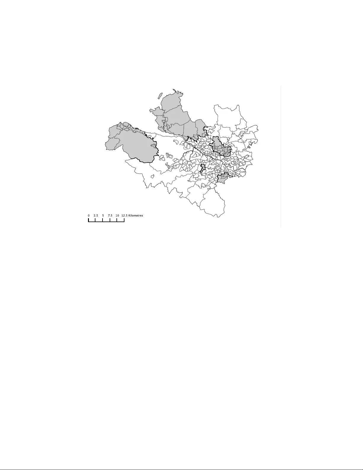
Loading comments...
Leave a Comment