Improved testing inference in mixed linear models

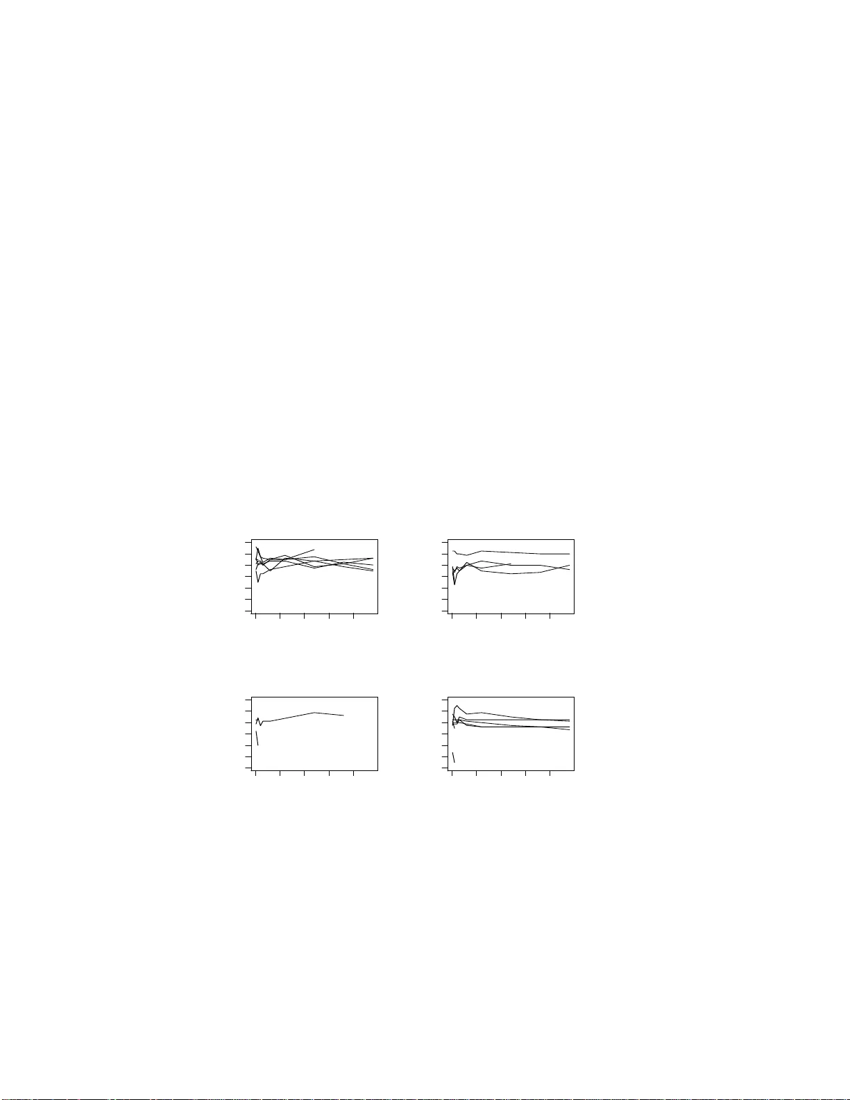
Impro v ed testing inferenc e in mixed linear mo dels T atia ne F. N. Melo, Silvi a L. P . F errari Dep ar tamento de Estat ´ ıstic a, Universidade de S˜ ao Paulo, R ua do Mat˜ ao , 101 0, S˜ ao Paulo/SP, 05508 -090, Br azil F rancisco Criba ri-Neto Dep ar tamento de Estat ´ ıstic a, Universidade F e der al de Pernambuc o, Cidade Universit´ aria, R e cife/PE, 50740-540 , B r azil Abstract Mixed linear mo dels are commonly used in rep eate d measures studies. Th e y accoun t for the dep endence amongst obs er v ations obtained fr om the same exp erimen tal unit. Often times, the n umb er of observ ati ons is small, and it is th us imp ortan t to u se inference strategies that incorp orate small sample corrections. In this p a p er, w e dev elop mod ified v ersions of the lik eliho od ratio test for fi xed effects inference in mixed lin ear mo dels. In particular, w e deriv e a Bartle tt correction to such a test and also t o a test obtained from a mo dified profile likelihoo d function. Ou r results generalize those in Zuc ker et al. ( Journal of the R oya l St atistic al So ciety B , 2000, 62 , 827–8 38) b y allo wing the parameter of int erest to b e vec tor-v alued. Additionally , our Bartlett c orrections allo w for r a nd om effects nonlinear co v ariance matrix structure. W e rep o rt sim ulation results wh ic h s h o w th a t the pr o p osed tests displa y sup erior finite sample b eha vior relativ e to the standard lik elihoo d ratio test. An application is also presented and discussed. Key wor ds: Bartlett correction, Fixed effects, Lik eliho od ratio test, Mixed linear mo dels, Mo dified pr ofi le like liho o d function. 1 In tro duction In recen t years repeated measures data hav e b een widely analyzed in man y fields, including biology and medicine. In suc h studies, the observ atio ns are obtained from differen t exp erime ntal units, eac h unit b eing observ ed mo r e than once (Brown and Prescott, 2006). In particular, some of these studies use Preprint sub mitte d to E lse vier 22 Marc h 2022 longitudinal data (V erb ek e and Molenberghs, 200 0), in whic h the o bs erv ations are collected ov er time. Mixed linear mo dels ha v e b een extensiv ely used b y practitioners to analyse rep eated measures since they a cc ount for within units correlation. It is also notew orthy that there is av ailable soft w are sp ecifically designed for the estimation of suc h mo dels ; see Pinheiro and Bates (2000) and Littel et al. (200 6). A common shortcoming lies in the fact that in man y studies the sample size is small whic h renders approximate inferential pro cedures unreliable. Impro v ed inference may b e based on the theory of higher order asymptotics. Practical applications of suc h theory ma y b e found in Brazzale et al. (200 7). The likeli- ho o d ratio test, which is commonly used to make inference on t he fixed effects parameters, quite oft en display s larg e size distortions when the sample size is small. This happ ens b ecause it s n ull distribution is p o orly approxim ated b y the limiting χ 2 distribution, fro m whic h critical v alues are obtained. It is p ossible to obtain a Ba rtlett correction f actor and use it to mo dify the lik eli- ho o d ratio test statistic in suc h a w a y to bring its n ull distribution closer to its limiting coun terpart; the appro ximation error is reduced from O ( n − 1 ) to O ( n − 2 ), where n is the sample size, thus making a n y size distortion v anish at a faster rate. Another shortcoming relates to the effect of the n uisance parameters o n the resulting inference on the parameters of in terest. D ifferen t mo difications to the profile lik eliho od function hav e b een prop osed with the aim of reducing suc h effect. F or a review see Sev erini (2000, Chapter 9); see also Sartori et al. (199 9 ) and Sartori (2 003). The adjustmen t prop osed b y Co x and Reid (1 987) can b e used whenev er the n uisance a nd interest parameters are orthogonal. DiCi- ccio and Stern (1994) ha v e sho wn that the Co x–Reid test statistic can be Bartlett-corrected, just a s t he lik eliho od ratio test statistic. The com bined use of mo dified profile likelihoo ds and Bartlett correction can deliv er accurate and reliable inference in small samples, as evidenc ed b y the results in F errari et al. (2004 ), F errari et al. (2 0 05) and Cysneiros and F errari (200 6). Zuc k er et a l. (2000 ) o btained improv ed lik eliho o d ra tio testing inference b y deriving Bartlett corrections to the profile and mo dified (Co x–Reid) profile lik eliho o d ratio tests on the fixed effects parameters in mixed linear mo d- els. Their results, ho w ev er, are only applicable for testing one parameter a t a time, since they only allo w fo r a scalar para me ter of in terest. In many studies, nonetheless, practitioners wish to p erform join t tes ting inference on a set of parameters, es p ecially when comparing three or more treatmen ts in medical trials. Also, they derive d t he Bartlett correction to the profile lik eliho o d ratio test only for the situation where the co v a r iance matrix fo r t he random effects has a linear structure. Hence, their results are not fully applicable in man y situations of inte rest, e.g. when the resp onses of a single sub ject are measured sequen tially and the errors are assumed to b e auto correlated. Our chief goal 2 is to generalize their results so that they a r e v a lid in situations where the pa- rameter of inte rest is v ector-v alued and the co v ariance matrix for the random effects is allow ed to ha ve a non-linear structure. W e obtain the Co x–Reid pro- file lik eliho o d adjustmen t, and also Bartlett correction factors for the pro file and adjusted profile like liho o d ratio t est statistics. The pap er unfolds as follo ws. Section 2 in tro duces the mixed linear mo del, Section 3 con tains the three improv ed t e sts (Cox–Reid and Bartlett-corrected tests), and Section 4 presen ts sim ulation study on the finite sample b eha vior of the standard like liho o d ratio test a nd its mo dified counterparts. An application that uses real data is presen ted and discus sed in Section 5 . Finally , Section 6 concludes the pap er. T ec hnical details are collected in tw o app endices . 2 Mixed linear mo dels The mixed linear mo del is given by y i = X i β + Z i b i + ǫ i , i = 1 , . . . , N , (1) where y i = ( y i 1 , y i 2 , . . . , y iτ i ) ⊤ is a τ i × 1 v ector of responses on the i th experi- men tal unit, β is a n n -v ector of fixed effects parameters, X i is a τ i × n known matrix, b i is a random effects v ector ( q × 1), Z i is a kno wn τ i × q matrix, and ǫ i = ( ǫ i 1 , ǫ i 2 , . . . , ǫ iτ i ) ⊤ is a τ i × 1 v ector of random errors. It is often times assumed that ǫ i ∼ N τ i ( 0 , σ 2 I τ i ), where I τ i denotes the τ i × τ i iden tit y ma- trix and 0 is a v ector of zeros. It is also assumed that b i ∼ N q ( 0 , G ), where b 1 , b 2 , . . . , b N , ǫ 1 , ǫ 2 , . . . , ǫ N are indep enden t and G = G (  ) is a q × q p ositiv e definite matr ix,  b eing an m × 1 v ector of unkno wn pa r amete rs. Mo del (1) can b e written in matrix form as Y = X β + Z b + ǫ, (2) where Y = ( y ⊤ 1 , y ⊤ 2 , . . . , y ⊤ N ) ⊤ is T × 1 , with T = P N i =1 τ i , X = ( X ⊤ 1 , X ⊤ 2 , . . . , X ⊤ N ) ⊤ is a T × n matrix, Z is a T × N q diago na l matrix giv en by Z = diag( Z 1 , Z 2 , . . . , Z N ), b = ( b ⊤ 1 , b ⊤ 2 , . . . , b ⊤ N ) ⊤ is an N q -v ector and ǫ = ( ǫ ⊤ 1 , ǫ ⊤ 2 , . . . , ǫ ⊤ N ) ⊤ is T × 1. Thus , b ∼ N N q ( 0 , I N ⊗ G ), where ⊗ denotes the Kronec k er pro duct a nd ǫ ∼ N T ( 0 , σ 2 I T ); b and ǫ are indep ende nt. It is p ossible to write mo del (2) as Y = X β + e , (3) where e = Z b + ǫ . Hence, e ∼ N T ( 0 , Σ ), where Σ = Σ ( ω ) = Z ( I N ⊗ G ) Z ⊤ + σ 2 I T , ω = (  ⊤ , σ 2 ) ⊤ b eing an ( m + 1) × 1 ve ctor of unkno wn parameters. 3 Hence, the log-likelihoo d function f o r mo del (3) can b e expressed as ℓ ( β , ω ; Y ) = − T 2 log(2 π ) − 1 2 log | Σ | − 1 2 ( Y − X β ) ⊤ Σ − 1 ( Y − X β ) , (4) where | · | denotes matrix determinan t. Let θ = ( ψ ⊤ , ς ⊤ , ω ⊤ ) ⊤ b e the ( n + m + 1)- v ector of parameters, where ψ = ( β 1 , β 2 , . . . , β p ) ⊤ is the p -vec tor ( p ≤ n ) con taining the first p elemen ts of β and ( ς ⊤ , ω ⊤ ) ⊤ is the ( n − p + m + 1) × 1 v ector of n uisance parameters with ς = ( β p +1 , β p +2 , . . . , β n ) ⊤ . In what follo ws w e shall fo cus on fixed effects inference. In particular, w e wish t o test H 0 : ψ = ψ (0) against H 1 : ψ 6 = ψ (0) , where ψ (0) is a giv en p - v ector. W e f o llo w Zuc k er et al. (2 000) and use a reparameterization in whic h the n uisance (( ς ⊤ , ω ⊤ ) ⊤ ) and interes t ( ψ ) para meters are ortho g onal. In particular, w e transform θ = ( ψ ⊤ , ς ⊤ , ω ⊤ ) ⊤ in to ϑ = ( ψ ⊤ , ξ ⊤ , ω ⊤ ) ⊤ , with ξ = ς + ( f X ⊤ n − p Σ − 1 f X n − p ) − 1 f X ⊤ n − p Σ − 1 f X p ψ , (5) where f X p denotes the matrix formed out of the first p columns of X and f X n − p con tains the remaining ( n − p ) columns of X . It is easy to show that ψ is orthogonal to φ = ( ξ ⊤ , ω ⊤ ) ⊤ , i.e., the exp ecte d v alues o f ∂ 2 ℓ ( ϑ ; Y ) /∂ ψ ∂ ξ ⊤ and ∂ 2 ℓ ( ϑ ; Y ) /∂ ψ ∂ ω j , for j = 1 , 2 , . . . , m + 1, are matr ic es of zeros. By partitioning X as ( f X p , f X n − p ) and β as ( ψ ⊤ , ς ⊤ ) ⊤ , w e can write X β = f X p ψ + f X n − p ς . Using (5) w e obta in X β = f X ′ p ψ + f X n − p ξ , where f X ′ p = [ I T − f X n − p ( f X ⊤ n − p Σ − 1 f X n − p ) − 1 f X ⊤ n − p Σ − 1 ] f X p . It follo ws t hat the log-lik eliho o d function in (4) can b e written as ℓ = ℓ ( ϑ ; Y ) = − T 2 log(2 π ) − 1 2 log | Σ | − 1 2 z ⊤ Σ − 1 z , (6) where z = z ( Y , X , ϑ ) = Y − f X ′ p ψ − f X n − p ξ . 3 Impro v ed lik eliho o d ratio tests 3.1 Bartlett c orr e c tion The profile lik eliho o d function, whic h only in v olve s the v ector of parameters of interes t, is defined as ℓ p ( ψ ) = ℓ ( ψ , b φ ( ψ )), where b φ ( ψ ) is the maximum lik eliho o d estimator of φ fo r a fixed v alue of ψ . The lik eliho o d ratio statistic 4 for testing H 0 is LR = LR ( ψ (0) ) = 2 n ℓ p ( b ψ ) − ℓ p ( ψ (0) ) o , where b ψ denotes the maxim um lik eliho o d estimator of ψ . Under the standard regularit y conditions a nd under H 0 , LR conv erg es in distribution to χ 2 p . This first order approximation ma y not work w ell in small s amples, ho w ev er. In order to a chiev e more accuracy , Bartlett (1937) prop osed m ultiplying LR by a constant, (1 + C /p ) − 1 , thus obtaining what is now know n as the Bartlett- corrected test statistic: LR ∗ = LR 1 + C /p , where C is a constan t of order n − 1 c hosen suc h that , under H 0 , E( LR ∗ ) = p + O ( n − 3 / 2 ). In regular problems, and unde r the n ull h yp othesis LR ∗ is χ 2 p distributed up to an error of order n − 2 ; see Bar ndo r ff - Niels en and Hall (1 988). A general express ion for C in terms of log-lik eliho o d c umulan t s up to the fourth order w as obtained b y Lawle y (1956). One of our goals is to obta in the Bartlett correction t erm C fo r testing H 0 : ψ = ψ (0) against H 1 : ψ 6 = ψ (0) for mixed linear mo dels . This is done in App endix A using Lawley’s results; see ( A.1 ). F o r simplicit y , here w e o nly giv e the expres sion for C when the ψ (0) = 0 , whic h is common in practical applications: C = tr  D − 1  − 1 2 M + 1 4 P − 1 2 ( γ + ν ) τ ⊤  , (7) where tr( · ) is the t r a ce op erator. Here, D , M and P a r e ( m + 1) × ( m + 1) matrices giv en by D = { (1 / 2 ) tr( ˙ Σ j ˙ Σ k ) } , M = { tr(( f X ′⊤ p Σ − 1 f X ′ p ) − 1 ( f X ′⊤ p ¨ Σ j k f X ′ p + 2 ˙ X ′⊤ k ˙ Σ j f X ′ p )) } , P = { tr(( f X ′⊤ p ˙ Σ j f X ′ p )( f X ′⊤ p Σ − 1 f X ′ p ) − 1 ( f X ′⊤ p ˙ Σ k f X ′ p )( f X ′⊤ p Σ − 1 f X ′ p ) − 1 ) } and τ , γ and ν are ( m + 1)-ve ctors whose j th elemen ts are tr(( f X ′⊤ p Σ − 1 f X ′ p ) − 1 ( f X ′⊤ p ˙ Σ j f X ′ p )), tr( D − 1 A ( j ) ) and tr(( f X ⊤ n − p Σ − 1 f X n − p ) − 1 ( f X ⊤ n − p ˙ Σ j f X n − p )), resp ec- tiv ely . Not e that we give the ( j, k ) eleme nt of eac h matrix. In our notation, A ( j ) is the ( m + 1) × ( m + 1) matrix giv en b y A ( j ) = { (1 / 2) tr ( ˙ Σ l ¨ Σ j k ) − (1 / 2) tr( ˙ Σ k ¨ Σ j l ) − (1 / 2) tr( ˙ Σ j ¨ Σ lk ) } . Also, ˙ Σ j = ∂ Σ /∂ ω j , ˙ Σ j = ∂ Σ − 1 /∂ ω j = − Σ − 1 ˙ Σ j Σ − 1 , ¨ Σ j k = ∂ 2 Σ /∂ ω j ∂ ω k , ¨ Σ j k = ∂ 2 Σ − 1 /∂ ω j ∂ ω k = − 2 ˙ Σ k ˙ Σ j Σ − 1 − Σ − 1 ¨ Σ j k Σ − 1 and ˙ X ′ j = ∂ f X ′ p /∂ ω j = − f X n − p ( f X ⊤ n − p Σ − 1 f X n − p ) − 1 f X ⊤ n − p ˙ Σ j f X ′ p . It is notew orth y that (7) generalizes the result in Zuc k er et al. (2000, eq. (3)). Their expres sion is only v alid when the parameter under test is scalar and the 5 co v a riance matrix for the random effects has a linear structure and so do es Σ , i.e., Σ = P ω j Q j , where Q j are known matrices. Note that when Σ has a linear structure we hav e ˙ Σ j = Q j , ∀ j, ¨ Σ j k = 0 , ∀ j, k , and equation (7 ) b ecomes C = tr  D − 1  − 1 2 M + 1 4 P − 1 2 ν τ ⊤  . (8) Additionally , when ψ is sc alar, our expression (8 ) reduce s to equation (3) in Zuc k er et al. (200 0 ). Also, when the n ull h yp othesis is H 0 : β = β (0) , (8 ) reduces to C = tr  D − 1  − 1 2 M 1 + 1 4 P 1  , where M 1 = { tr(( X ⊤ Σ − 1 X ) − 1 ( X ⊤ ¨ Σ j k X )) } and P 1 = { tr(( X ⊤ ˙ Σ j X )( X ⊤ Σ − 1 X ) − 1 ( X ⊤ ˙ Σ k X )( X ⊤ Σ − 1 X ) − 1 ) } . 3.2 Cox–R eid pr ofile likeliho o d a d just ment Co x a nd Reid (1987) prop osed an adjustmen t to the pro file like liho o d function whic h can b e used when the nuis ance and in terest parameters are orthogona l. The Co x–Reid adjusted profile log-like liho o d function is giv en by ℓ pa ( ψ ) = ℓ p ( ψ ) − 1 2 log n    − ℓ φφ  b φ ( ψ )     o , where ℓ φφ is the matrix of second deriv ativ es o f ℓ with resp ect to φ . The corresp onding lik eliho o d rat io t est stat istic is LR C R ( ψ (0) ) = 2 n ℓ pa ( e ψ ) − ℓ pa ( ψ (0) ) o , where e ψ is the maximizer of ℓ pa ( ψ ). The Cox–Reid test statistic is χ 2 p distributed under H 0 up to an error of order n − 1 , just lik e the standard likelihoo d ratio test statistic . DiCiccio and Stern (1994) defined a Ba rtlett correction to this test statistic whic h reduces the order of the approximation error to O ( n − 2 ). The corrected t es t stat istic is LR ∗ C R = LR C R 1 + C ∗ /p , where C ∗ is a constant of order n − 1 suc h that, under H 0 , E( LR ∗ C R ) = p + O ( n − 3 / 2 ). A general express ion for C ∗ can b e found in DiCiccio and Stern (1994, eq. (25)). In App endix B, w e obtain C ∗ for testing H 0 in mixed linear mo dels ; 6 see (B.1). Here, we giv e the expression for C ∗ for the case where ψ (0) = 0 : C ∗ = tr  D − 1  − M + 1 4 P + γ ∗ τ ⊤  , (9) where D , M , P and τ w ere giv en ab ov e a nd the j th elemen t o f t he v ector γ ∗ is tr( D − 1 C ( j ) ), with C ( j ) b eing an ( m + 1) × ( m + 1) matrix g iven b y C ( j ) = {− tr( ˙ Σ k ˙ Σ j Σ − 1 ˙ Σ l ) + ( 1 / 2) tr( ˙ Σ j ¨ Σ k l ) + (1 / 2) t r( ˙ Σ k ¨ Σ j l ) } . Our expres sion for C ∗ generalizes the result in Z uc ker et al. (2000, eq. (4)), since their form ula is o nly v alid when p = 1. W e notice that their formula re- mains v a lid when t he co v aria nc e mat r ix for the random effects has a nonlinear structure. As exp ected, (9) reduces to equation (4) of Zuck er et al. (200 0) when p = 1. Also, for testing H 0 : β = β (0) against H 1 : β 6 = β (0) , C ∗ reduces to (9) with M and P replaced by M 1 and P 1 , resp ective ly , and τ replaced by τ 1 , with τ 1 b eing the ( m + 1 )-v ector whose j th elemen t is tr(( X ⊤ Σ − 1 X ) − 1 ( X ⊤ ˙ Σ j X )). The expressions we g iv e for C and C ∗ in (7) and (9), r esp ectiv ely , only in v olv e simple o p erations on vec tors and matrices. Therefore, they can b e easily com- puted with t he aid of a programming language or soft w are whic h can p erform suc h op erations, e.g. Ox (Cribari-Neto a nd Zarkos, 2 0 03; Do ornik, 2006) and R (Ihak a and Gen tleman, 19 96). W e note that C and C ∗ only dep end on X , on the inv erse cov ariance matrix Σ − 1 , on t he co v aria nc e matrix Σ a nd its first t w o deriv ativ es with respect to ω . 4 Sim ulation study In this section w e shall presen t the res ults of Mon te Carlo sim ulat io n exper- imen ts in whic h w e ev aluate the finite sample p erformances of the lik eliho o d ratio test ( LR ), its Bartlett-corrected v ersion ( LR ∗ ), t he adjusted profile lik e- liho o d ratio test ( LR C R ) a nd its Bartlett- correcte d counterpart ( LR ∗ C R ). The sim ulations w ere based on the fo llo wing mixed linear mo del: y ij = β 0 + β 1 t ij + β 2 x 1 i + β 3 x 2 i + b 0 i + b 1 i t ij + ǫ ij , for j = 1 , 2 , . . . , τ i with τ i ∈ { 2 , 3 , 4 , 5 , 6 , 7 , 8 , 9 } and i = 1 , 2 , . . . , N . The v a lues of t ij w ere obtained as random dra ws from the standard uniform distribution U (0 , 1); x 1 i and x 2 i are dumm y v ariables. The fixed effects parameters are β 0 , β 1 , β 2 , β 3 . Also, b i = ( b 0 i b 1 i ) ⊤ ∼ N 2 ( 0 , G ) with G =    ω 1 ω 2 ω 2 ω 3    . (10) 7 Additionally , the ǫ ij ’s are independen t from the b i ’s, and ǫ i ∼ N τ i (0 , ω 4 I τ i ). W e test H 0 : ψ = 0 against H 1 : ψ 6 = 0 , where ψ = ( β 2 β 3 ) ⊤ . All simulations w ere p erformed using the Ox matrix pro gramming language (Cribari-Neto and Zark os, 2003; D oornik, 2006 ). The num b er of Mon te Carlo replications w as 5 ,0 00 and the sample sizes considere d w ere N = 1 2 , 24 and 36. The parameter v alues are β 0 = 0, β 1 = 0 . 2, β 2 = 0, β 3 = 0, ω 1 = 1, ω 2 = 0 and 0 . 2 5, ω 3 = 0 . 5 and 1, and ω 4 = 0 . 05. All tests w ere carried out at the follo wing nominal lev els: α = 5% and α = 10%. The null rejection r ates of the four tests under ev aluation are displa y ed in T able 1. W e note that the lik eliho o d ra tio test is lib eral. F or instance, when ω 2 = 0, ω 3 = 0 . 50, N = 12 a nd α = 10%, its rejection rate exceeds 20%. It is notew orth y that the t hree alternativ e tests o ut p erform the standard lik eliho o d ratio test. F or N = 12 and N = 24, the t w o best p erforming tests a re LR C R and LR ∗ C R ; LR ∗ is s lightly ov ersized. F or example, when ω 2 = 0, ω 3 = 0 . 50, N = 1 2 and α = 5 %, the null rejection r ates of LR C R , LR ∗ C R and LR ∗ are, resp ectiv ely , 4 . 5%, 5 . 3% and 7 . 6% ( LR : 13 . 0%). It is not p ossible to single out a global winner b et w een LR C R and LR ∗ C R . When N = 36, the Co x–Reid a nd the t wo Bartlett-corrected tests still o utperform LR ; here, LR ∗ sligh tly outp erforms the other tw o a lt e rnative tests, LR ∗ C R b eing the sec ond b est p erforming test. T able 1 Null rejection rates of the tests of H 0 : ψ = 0 ; en tries are p ercen tages. α = 5% α = 10% N ω 2 ω 3 LR LR ∗ LR C R LR ∗ C R LR LR ∗ LR C R LR ∗ C R 12 0 0.50 13.0 7.6 4.5 5.3 20.8 13.1 9.2 10.2 0 1 13.4 7.8 4.8 5.9 21.7 13.5 9.6 10.8 0.25 0.50 11.2 6.0 3.4 4.1 19.0 11.2 7.5 8.5 0.25 1 13 .8 7.9 5.1 5.8 21.9 13.9 9.6 10.7 24 0 0.50 8.3 5.6 4.7 5.0 14.6 10.9 9.5 10.0 0 1 8.5 5.8 4.9 5.1 14.6 11.1 10.1 10.5 0.25 0.50 8.6 5.7 4.8 5.1 14.8 11.1 9.6 10.2 0.25 1 8.7 6.0 4.8 5.1 15.0 11.4 10 .1 10.6 36 0 0.50 6.4 4.6 4.2 4.4 12.8 10.1 9.5 9.8 0 1 6.1 4.9 4.4 4.7 12.6 9.8 9.0 9.4 0.25 0.50 6.7 4.8 4.3 4.6 12.4 10.0 9.3 9.6 0.25 1 6.4 4.7 4.3 4.4 12.6 9.8 9.1 9.4 Figure 1 plots the relativ e quan tile discrepancies against the a s ymptotic quan- tiles for N = 12, the smallest sample size, where the corrections ar e mostly needed. Relativ e quan tile discrepancies are defined as differences b et w een ex- act and asymptotic ( χ 2 2 ) quan tiles divided b y the latter. The closer to zero these discrepancies, the b etter the approxim ation used in the test. W e note 8 that the test statistics with the smallest relat ive quan tile discrepancies ar e LR C R and LR ∗ C R . W e also note that quan tiles of LR are approximately 50% larger than the resp ectiv e asymptotic ( χ 2 2 ) quan tiles. 2 4 6 8 0.0 0.2 0.4 0.6 0.8 2 4 6 8 0.0 0.2 0.4 0.6 0.8 2 4 6 8 0.0 0.2 0.4 0.6 0.8 Asymptotic quantile Relative quantile discrepancy 2 4 6 8 0.0 0.2 0.4 0.6 0.8 Asymptotic quantile Relative quantile discrepancy LR LR* LR CR LR CR * Fig. 1. Relativ e quantil e d iscrepancies p lot : N = 12, ω 2 = 0 and ω 3 = 0 . 50. Note that the sim ulated model a nd the hy p othesis under test ha v e practical applications, fo r instance, when the practitioner wishes to compare tw o differ- en t tr e atments and the exp erimen tal units are observ ed in differen t p oin ts in time. Here , w e assume that the time horizon of the stud y is limited. This is wh y w e used a b ounded distribution fo r c ho osing v a lues for t ij . W e p erformed sim ulations under other situatio ns . W e v aried the v a lues of all the parame- ters and considered a gamma distribution with mean 3 and v aria nc e 1 . 5 for c ho osing v alues fo r t ij . Also, w e considered an extende d mo del in whic h in- teractions b et w een t ij and the dumm y v ariables w ere included. In this case , w e tested the interactions effects. F o r the sak e of brevity , the results are not sho wn. In short, the Co x–Reid and the t w o Bartlett-corrected tests outp er- formed LR . F or instance, our sim ulation exp erimen t with β 0 = 0 . 2, β 1 = 0 . 4, β 2 = β 3 = 0, ω 1 = 1 . 5, ω 2 = 0 . 05, ω 3 = 1 . 2, ω 4 = 0 . 10 and N = 24 y ielded the followin g null rejection rates at t he 10 % nominal lev el: 14 . 7% ( LR ), 10 . 6% ( LR ∗ ), 9 . 4% ( LR C R ) and 9 . 8% ( LR ∗ C R ). Also, for an extended mo del whic h includes tw o pa rameters , β 4 and β 5 , represen ting inte ractions b et w een t ij and the dumm y v aria ble s, w e obtained 7 . 1% ( LR ), 5 . 4% ( LR ∗ ), 3 . 3% ( LR C R ) and 5 . 0% ( LR ∗ C R ) for α = 5 % and N = 24. Here, β 0 = 0 . 2, β 1 = 0 . 4, β 2 = 0 . 3, β 3 = 0 . 5, β 4 = β 5 = 0 and the same v alues for ω 1 , . . . , ω 4 as b efore. 9 5 Blo o d pressure data W e shall now presen t an application that uses a r e al data set. The data consist of a randomly selected subset of the data used by Crep eau et al. (19 85). Heart attac ks w ere induced in rats exp osed to four differen t low concen t r ations of halothane; group 1: 0% (con trol), group 2: 0.25%, group 3: 0 .50% and group 4: 1.0%. Our sample consists of 23 rats. The blo o d pressure of eac h rat (in mm Hg) is recorded ov er differen t p oin ts in time, from 1 to 9 recordings, a fter the induced heart atta ck. The main goal is to inv estigate the effect of halothane on the blo o d pressure. Figure 2 sho ws plo ts of blo o d pressure vers us time for eac h rat. Clearly , the profiles differ on the intercept. Ho w ev er, the slop es are no t mark edly different. A t the outset, w e consider a mo del where blo o d pressure v aries linearly with time, p ossibly with differen t in tercepts and slop es for each concen tration of halothane, and with in tercept and slop e ra ndom effects to accoun t for animal- to-animal v aria tion. As w e will see la ter, the usual lik eliho o d rat io test rejects the n ull h yp othesis of comm on slop e at the 10% no minal leve l, unlik e the mo dified tests. 0 50 100 150 200 20 40 60 80 100 120 140 0 50 100 150 200 20 40 60 80 100 120 140 0 50 100 150 200 20 40 60 80 100 120 140 0 50 100 150 200 20 40 60 80 100 120 140 0 50 100 150 200 20 40 60 80 100 120 140 0 50 100 150 200 20 40 60 80 100 120 140 0 50 100 150 200 20 40 60 80 100 120 140 Group 1 Time Blood pressure 0 50 100 150 200 20 40 60 80 100 120 140 0 50 100 150 200 20 40 60 80 100 120 140 0 50 100 150 200 20 40 60 80 100 120 140 0 50 100 150 200 20 40 60 80 100 120 140 0 50 100 150 200 20 40 60 80 100 120 140 0 50 100 150 200 20 40 60 80 100 120 140 Group 2 Time Blood pressure 0 50 100 150 200 20 40 60 80 100 120 140 0 50 100 150 200 20 40 60 80 100 120 140 0 50 100 150 200 20 40 60 80 100 120 140 Group 3 Time Blood pressure 0 50 100 150 200 20 40 60 80 100 120 140 0 50 100 150 200 20 40 60 80 100 120 140 0 50 100 150 200 20 40 60 80 100 120 140 0 50 100 150 200 20 40 60 80 100 120 140 0 50 100 150 200 20 40 60 80 100 120 140 0 50 100 150 200 20 40 60 80 100 120 140 0 50 100 150 200 20 40 60 80 100 120 140 Group 4 Time Blood pressure Fig. 2. Blo o d pressure against time for eac h rat. The mixed linear mo del considered here is y ij = β 0 + β 1 t ij + γ 02 G 2 i + γ 03 G 3 i + γ 04 G 4 i + γ 12 G 2 i t ij + γ 13 G 3 i t ij + γ 14 G 4 i t ij + b 0 i + b 1 i t ij + ǫ ij , (11) with i = 1 , 2 , . . . , 23 and j = 1 , 2 , . . . , τ i , where y ij is the blo od pressure of the i th rat at time j , t ij is the j th p oin t in time (in min utes) in whic h the i th rat 10 blo o d pressure w as recorded, a nd G 2 i is a dummy v a riable that equals 1 if the i th rat b elongs to g roup 2 and 0 otherwise. Also, G 3 i and G 4 i equal 1 for groups 3 a nd 4, respective ly . W e a ss ume that b i = ( b 0 i b 1 i ) ⊤ i . i . d . ∼ N 2 ( 0 , G ), where G is giv en in (10). Additionally , ǫ ij i . i . d . ∼ N (0 , ω 4 ), t he ǫ ij ’s b eing indep enden t of the b i ’s. The maxim um lik eliho od estimates of the fixed effects parameters are b β 0 = 104 . 360, b β 1 = 0 . 004, b γ 02 = − 0 . 719, b γ 03 = 0 . 203, b γ 04 = − 15 . 2 11, b γ 12 = 0 . 022, b γ 13 = 0 . 109 and b γ 14 = − 0 . 019. W e wish to make inference on γ 12 , γ 13 and γ 14 . More sp ec ifically , w e wish t o test H 0 : ψ = 0 against H 1 : ψ 6 = 0 , where ψ = ( γ 12 , γ 13 , γ 14 ) ⊤ . Note that under the n ull h yp othesis , the mean slop es are equal fo r the differen t halot ha ne concentrations. The adjusted profile maxim um like liho o d estimates of γ 12 , γ 13 and γ 14 are e γ 12 = 0 . 020, e γ 13 = 0 . 101 and e γ 14 = − 0 . 030, resp ectiv ely . The test statistics assume the following v alues: LR = 6 . 522 ( p -v a lue : 0.089), LR ∗ = 5 . 6 78 ( p -v alue: 0.128), LR a = 5 . 287 ( p - v alue: 0 . 152) and LR ∗ C R = 6 . 168 ( p - v alue: 0 . 104). The standard lik eliho o d r a tio test rejects the n ull h yp othesis at the 10% nominal lev el, i.e., it suggests that there are differences in mean slop es for differen t dosages. The three mo dified tests, ho w ev er, suggest otherwise, i.e., the null hypothesis is not rejected b y these tests at the same nominal lev el. W e now consider the fo llo wing reduced mo de l: y ij = β 0 + β 1 t ij + γ 02 G 2 i + γ 03 G 3 i + γ 04 G 4 i + b 0 i + b 1 i t ij + ǫ ij , with i = 1 , 2 , . . . , 23 and j = 1 , 2 , . . . , τ i . W e wish t o test H ∗ 0 : ψ ∗ = 0 against H ∗ 1 : ψ ∗ 6 = 0 , where ψ ∗ = ( γ 02 , γ 03 , γ 04 ) ⊤ . Not e t ha t we are testing whether the mean blo o d pressures are equal across the differen t dosages. The fixed effects maxim um lik eliho o d estimates are b β 0 = 99 . 53 1 , b β 1 = 0 . 006 , b γ 02 = − 0 . 525, b γ 03 = 2 . 318 and b γ 04 = − 13 . 357 . The adjusted profile maxim um lik eliho o d estimates of γ 02 , γ 03 and γ 04 are, resp ectiv ely , e γ 02 = − 0 . 823, e γ 03 = 2 . 07 9 and e γ 04 = − 12 . 573. W e no w ha v e LR = 6 . 143 ( p -v alue: 0 . 105), LR ∗ = 5 . 174 ( p -v alue: 0 . 159), LR a = 4 . 002 ( p -v alue: 0 . 2 61) and LR ∗ C R = 4 . 167 ( p -v alue: 0 . 244). All tests yield t he same inference, namely: the n ull h yp othesis is not rejected at the 10% nominal lev el. Therefore, w e conclude tha t there is no group effect. In other w ords, the a nal- ysis carried out using the mo difie d tests suggests that the blo od pressure is not affected by the administration o f halothane at the concentrations consid- ered in the experimen t. This conclusion agrees with the findings of Crep eau et al. (1985). 11 6 Concluding remarks W e a ddressed the issue of p erforming like liho o d-based testing inference on the fixed effects parameters of mixed linear mo dels when the sample con tains a small n um b er of observ atio ns . The standard like liho o d ratio test is lib eral, as evidenced b y our Monte Carlo results. W e obtained three a lternativ e tests, namely: an adjusted pro file like liho o d ratio test, its Bartlett-corrected v ersion and also the Bartlett-corrected lik elihoo d r a tio test. Our results generalize those in Zuck er et al. (2000) in t w o directions. First, w e a llo w practitioners to test joint restrictions on one or more fixed effects parameters, whereas their results only hold for t ests on a parameter at a time. Second, unlik e Zuc k er et al. (2 000), w e do no t assume that the co v ariance matrix o f the random effects is linear when deriving t he Bartlett correction to the profile lik eliho o d ratio test. Our main results a re stated t hrough closed-form formulas that only inv o lve simple op erations on v ectors and matrices, and hence they can be easily implemen ted in matrix programming languages and statistical soft w are. The sim ulation study w e rep ort clearly sho w that the prop osed tests outp erform the standard lik eliho o d ratio test, esp ecially when the sample size is small. It shows that the three alternativ e tests yield reliable inferences ev en for unbalanced data . In particular, the adjusted profile like liho o d ratio test and its Bartlett-corrected vers ion improv e t he t ype I error rate, esp ecially when the nu mber of o bs erv ations is small. Ac kno wledgemen ts W e gratefully ac know ledge financial supp ort from F AP ESP and CNPq. W e also thank three anonymous referees for helpful suggestions. App endix A . Deriv ation of C W e use the follo wing tensor notation for log-lik eliho od cum ulan ts: κ r s = E  ∂ 2 ℓ ∂ ϑ r ∂ ϑ s  , κ r st = E  ∂ 3 ℓ ∂ ϑ r ∂ ϑ s ∂ ϑ t  and κ r stu = E  ∂ 4 ℓ ∂ ϑ r ∂ ϑ s ∂ ϑ t ∂ ϑ u  , ϑ r b eing the r th element of ϑ . Th e notation used for deriv ativ es of cumulan ts is the follo wing: ( κ r s ) t = ∂ κ r s ∂ ϑ t , ( κ r st ) u = ∂ κ r st ∂ ϑ u and ( κ r s ) tu = ∂ κ r s ∂ ϑ t ∂ ϑ u . 12 In what follo ws, we sh al l use similar notatio n for deriv ativ es of matrices formed out of cum ulan ts. Note that − κ r s is the ( r , s ) elemen t of Fisher’s information matrix; the ( r , s ) element of its in ve rse is denoted by − κ r s . La wley’s (1956) formula for C is C = X ψ, ξ,ω ( l r stu − l r stuvw ) − X ξ ,ω ( l r stu − l r stuvw ) = C 1 − C 2 , where C 1 = P ψ, ξ,ω l r stu − P ξ ,ω l r stu and C 2 = P ψ, ξ,ω l r stuvw − P ξ ,ω l r stuvw with l r stu = κ r s κ tu  1 4 κ r stu − ( κ r st ) u − ( κ r t ) su  and l r stuvw = κ r s κ tu κ vw ( κ r t v  1 6 κ suw − ( κ sw ) u  + κ r t u  1 4 κ svw − ( κ sw ) v  + ( κ r t ) v ( κ sw ) u + ( κ r t ) u ( κ sw ) v ) , where the indices r, s, t, u, v , w refer to the comp onen ts of ϑ = ( ψ ⊤ , ξ ⊤ , ω ⊤ ) ⊤ . Here, P ψ, ξ,ω denotes sum mat ion o v er all p ossible com binations of the n + m + 1 parameters in ϑ , and P ξ ,ω denotes summation ov er the com binations of the n − p + m + 1 parameters in ( ξ ⊤ , ω ⊤ ) ⊤ . W e use indices a, b, c, d in reference to the comp onen ts of ψ , ind ic es f , g for th e comp onen ts of ξ , and indices j, k , l, o for the elemen ts of ω . F ur ther n otation used here is giv en in Sections 2 and 3. The first-order deriv ativ es of th e log-lik eliho o d f u nctio n in (6) are ∂ ℓ ( ϑ ; Y ) ∂ ψ = e X ′⊤ p Σ − 1 z , ∂ ℓ ( ϑ ; Y ) ∂ ξ = e X ⊤ n − p Σ − 1 z , ∂ ℓ ( ϑ ; Y ) ∂ ω j = − 1 2 tr( Σ − 1 ˙ Σ j ) − 1 2 z ⊤ ˙ Σ j z + ψ ⊤ ˙ X ′⊤ j Σ − 1 z . The second-order deriv ativ es are ∂ 2 ℓ ( ϑ ; Y ) ∂ ψ ∂ ψ ⊤ = − e X ′⊤ p Σ − 1 e X ′ p , ∂ 2 ℓ ( ϑ ; Y ) ∂ ξ ∂ ξ ⊤ = − e X ⊤ n − p Σ − 1 e X n − p , ∂ 2 ℓ ( ϑ ; Y ) ∂ ψ ∂ ξ ⊤ = 0 , ∂ 2 ℓ ( ϑ ; Y ) ∂ ψ ∂ ω j = ( ˙ X ′⊤ j Σ − 1 + e X ′⊤ p ˙ Σ j ) z , ∂ 2 ℓ ( ϑ ; Y ) ∂ ξ ∂ ω j = e X ⊤ n − p ˙ Σ j ( Y − e X n − p ξ ) , ∂ 2 ℓ ( ϑ ; Y ) ∂ ω j ∂ ω k = − 1 2 tr( ˙ Σ j ˙ Σ k ) − 1 2 tr( Σ − 1 ¨ Σ j k ) − ψ ⊤ ˙ X ′⊤ k Σ − 1 ˙ X ′ j ψ + ψ ⊤ ( ¨ X ′⊤ j k Σ − 1 + ˙ X ′⊤ k ˙ Σ j + ˙ X ′⊤ j ˙ Σ k ) z − 1 2 z ⊤ ¨ Σ j k z , where ¨ X ′ j k = ∂ ˙ X ′ j ∂ ω k = 2 e X n − p ( e X ⊤ n − p Σ − 1 e X n − p ) − 1 e X ⊤ n − p ˙ Σ k e X n − p ( e X ⊤ n − p Σ − 1 e X n − p ) − 1 e X ⊤ n − p ˙ Σ j e X ′ p − e X n − p ( e X ⊤ n − p Σ − 1 e X n − p ) − 1 e X ⊤ n − p ¨ Σ j k e X ′ p . 13 Additionally , the third -o rd er deriv ativ es are ∂ 3 ℓ ( ϑ ; Y ) ∂ ξ ∂ ξ ⊤ ∂ ω j = − e X ⊤ n − p ˙ Σ j e X n − p , ∂ 3 ℓ ( ϑ ; Y ) ∂ ψ ∂ ψ ⊤ ∂ ω j = − e X ′⊤ p ˙ Σ j e X ′ p , ∂ 3 ℓ ( ϑ ; Y ) ∂ ψ ∂ ξ ⊤ ∂ ξ f = ∂ 3 ℓ ( ϑ ; Y ) ∂ ψ ∂ ξ ⊤ ∂ ω j = 0 , ∂ 3 ℓ ( ϑ ; Y ) ∂ ξ ∂ ω j ∂ ω k = e X ⊤ n − p ¨ Σ j k ( Y − e X n − p ξ ) , ∂ 3 ℓ ( ϑ ; Y ) ∂ ψ ∂ ω j ∂ ω k = ( ¨ X ′⊤ j k Σ − 1 + ˙ X ′⊤ k ˙ Σ j + ˙ X ′⊤ j ˙ Σ k + e X ′⊤ p ¨ Σ j k ) z , ∂ 3 ℓ ( ϑ ; Y ) ∂ ω j ∂ ω k ∂ ω l = − 1 2 ( tr( ¨ Σ lk ˙ Σ j ) + tr( ˙ Σ k ¨ Σ lj ) + tr( ˙ Σ l ¨ Σ j k ) + tr( Σ − 1 ¨ Σ j k l ) + z ⊤ ¨ Σ j k l z ) + ψ ⊤ ( ¨ X ′⊤ lk ˙ Σ j + ˙ X ′⊤ k ¨ Σ lj + ¨ X ′⊤ j k ˙ Σ l + ¨ X ′⊤ lj ˙ Σ k + ˙ X ′⊤ j ¨ Σ lk + ˙ X ′⊤ l ¨ Σ k j + ¨ X ′⊤ j k l Σ − 1 ) z , where ¨ Σ j k l = ∂ ¨ Σ j k /∂ ω l and ¨ X ′ j k l = ∂ ¨ X ′ j k /∂ ω l . Finally , the fourth-order d er iv ativ es can b e sh o w n to b e ∂ 4 ℓ ( ϑ ; Y ) ∂ ψ ∂ ψ ⊤ ∂ ω j ∂ ω k = − 2 ˙ X ′⊤ k ˙ Σ j e X ′ p − e X ′⊤ p ¨ Σ j k e X ′ p , ∂ 4 ℓ ( ϑ ; Y ) ∂ ψ ∂ ψ ⊤ ∂ ξ f ∂ ξ g = ∂ 4 ℓ ( ϑ ; Y ) ∂ ψ ∂ ψ ⊤ ∂ ξ f ∂ ω j = ∂ 3 ℓ ( ϑ ; Y ) ∂ ψ ∂ ψ ⊤ ∂ ξ f = 0 . T aking exp ected v alues of second, third and fourth deriv ativ es, we obtain K ψψ = E  ∂ 2 ℓ ( ϑ ; Y ) ∂ ψ ∂ ψ ⊤  = − e X ′⊤ p Σ − 1 e X ′ p , K ξ ξω j = E  ∂ 3 ℓ ( ϑ ; Y ) ∂ ξ ∂ ξ ⊤ ∂ ω j  = − e X ⊤ n − p ˙ Σ j e X n − p , K ψψ ω j ω k = E  ∂ 4 ℓ ( ϑ ; Y ) ∂ ψ ∂ ψ ⊤ ∂ ω j ∂ ω k  = − 2 ˙ X ′⊤ k ˙ Σ j e X ′ p − e X ′⊤ p ¨ Σ j k e X ′ p . In similar fashion, it follo ws that K ξ ξ = − e X ⊤ n − p Σ − 1 e X n − p , K ξ ω j = e X ⊤ n − p ˙ Σ j e X ′ p ψ , K ψω j = 0 , K ψψ ω j = − e X ′⊤ p ˙ Σ j e X ′ p , K ψξ ξ f = K ψξ ω j = 0 , K ψω j ω k = 0 , K ξ ω j ω k = e X ⊤ n − p ¨ Σ j k e X ′ p ψ , K ψψ ξ f ξ g = K ψψ ξ f ω j = 0 . Additionally , κ j k = 1 2 tr( ˙ Σ j ˙ Σ k ) − ψ ⊤ ˙ X ′⊤ j Σ − 1 ˙ X ′ k ψ , κ lj k = − 2 tr( ˙ Σ l ˙ Σ k Σ − 1 ˙ Σ j ) + 1 2 tr( ˙ Σ j ¨ Σ lk ) + 1 2 tr( ˙ Σ k ¨ Σ lj ) + 1 2 tr( ˙ Σ l ¨ Σ j k ) . Consider the follo wing matrices formed out of minus Fisher’s information in v erse: K ψψ = K − 1 ψψ , K ω ω = ( K ω ω − K ⊤ ξ ω K − 1 ξ ξ K ξ ω ) − 1 , K ξ ξ = K − 1 ξ ξ + K − 1 ξ ξ K ξ ω K ω ω K ⊤ ξ ω K − 1 ξ ξ and K ξ ω = K ω ξ ⊤ = − K − 1 ξ ξ K ξ ω K ω ω ⊤ , w here the j th column of K ξ ω is K ξ ω j and the ( j, k )th elemen t of K ω ω is κ j k . It can b e sho wn that ( K ψψ ) j = − e X ′⊤ p ˙ Σ j e X ′ p , ( K ψψ ) j k = − 2 ˙ X ′⊤ k ˙ Σ j e X ′ p − e X ′⊤ p ¨ Σ j k e X ′ p , ( K ξ ξ ) j = − e X ⊤ n − p ˙ Σ j e X n − p , ( K ξ ω j ) k = e X ⊤ n − p ¨ Σ j k e X ′ p ψ + e X ⊤ n − p ˙ Σ j ˙ X ′ k ψ , ( κ j l ) k = − tr( ˙ Σ l ˙ Σ j Σ − 1 ˙ Σ k ) + 1 2 tr( ˙ Σ j ¨ Σ lk ) + 1 2 tr( ˙ Σ l ¨ Σ j k ) . 14 It follo ws f r om the orth o gonalit y b et w een ψ and ( ξ ⊤ , ω ⊤ ) ⊤ that κ af = κ aj = ( κ af ) j b = ( κ aj ) f b = 0. Also, κ j f a = κ j f ab = 0. Hence, C 1 = X ( l abcd + l abf g + l abf j + l abj f + l abj k + l f g ab + l j k ab ) , where P ranges o v er all parameter combinatio ns indu ce d by the indices a, b, c, d, f , g , j, k . It is p ossible to sho w that l abcd = l abf g = l abf j = l abj f = l f g ab = 0. Thus, C 1 = X ( l abj k + l j k ab ) = X  κ ab κ j k  1 4 κ abj k − ( κ abj ) k  + 1 4 κ j k κ ab κ j k ab  . Since κ abj k = ( κ abj ) k = κ j k ab , C 1 reduces to C 1 = − 1 2 X κ ab κ j k κ abj k . As for C 2 , w e hav e that C 2 = X ( l abcd j k + l abj k cd + l j k loab + l j k ablo + l j k abcd + l f j g kab + l f j k gab + l f j k lab + l j k f g ab + l j k f l ab + l j k lf ab + l j f abg k + l j f abk g + l j f abk l + l j k abf g + l j k abf l + l j k ablf ) = X n − 1 4 κ ab κ cd κ j k κ abj κ cdk + 1 2 κ ab κ f g κ j k κ abj κ f g k − κ ab κ f j κ k l κ abj  2( κ f k ) l − 3 2 κ f k l  + 1 2 κ ab κ j k κ lo κ abj  κ k lo − 2( κ k l ) o  o . Therefore, C r educes to C = X n − 1 2 κ ab κ j k κ abj k + 1 4 κ ab κ cd κ j k κ abj κ cdk − 1 2 κ ab κ j k κ lo κ abj ( κ lok − 2( κ lo ) k ) + κ ab κ f k κ j l κ abj  2( κ f k ) l − 3 2 κ f k l  − 1 2 κ ab κ f g κ j k κ abj κ f g k o . W e no w arrive at the matrix expression give n by C = tr  K ω ω  − 1 2 M + 1 4 P −  1 2 ρ − δ + 1 2 η  τ ⊤  . (A . 1) Here, ρ , δ and η are ( m +1)-v ectors w hose j th elements are, resp ectiv ely , tr( K ω ω A ( j ) ), tr( K ξ ω ⊤ B ( j ) ) and tr( − K ξ ξ ( e X ⊤ n − p ˙ Σ j e X n − p )). In our notation, B ( j ) is a m a trix th at con tains the m + 1 column v ectors (1 / 2 e X ⊤ n − p ¨ Σ j k e X ′ p + 2 e X ⊤ n − p ˙ Σ j ˙ X ′ k ) ψ and A ( j ) is defined in Section 3.1. F or testing H 0 : ψ = 0 , C reduces to equ at ion (7). App endix B . Deriv ation of C ∗ W e sh al l now obtain C ∗ , whic h is used to Bartlett-c orrect the adju s te d profile lik e- liho od ratio test statistic. DiCiccio and Stern (1994, eq. (25)) giv e the follo wing 15 general expression: C ∗ = X ψ, ξ,ω ( 1 4 τ r u τ st κ r stu − κ r u τ st ( κ r st ) u +  κ r u κ st − ν r u ν st  ( κ r s ) tu −  1 4 κ r u τ st τ vw + 1 2 κ r u τ sw τ tv − 1 3 τ r u τ sw τ tv  κ r st κ uvw +  κ r u τ st κ vw + κ r u κ sw κ tv − ν r u κ sw ν tv  κ r st ( κ uv ) w −  κ r u κ st κ vw − ν r u ν st ν vw  ( κ r s ) t ( κ uv ) w −  κ r u κ sw κ tv − ν r u ν sw ν tv  ( κ r s ) t ( κ uv ) w ) , where ν r s = κ r s − τ r s , τ r s = κ r b κ sa σ ab , σ ab b eing the ( a, b ) elemen t of the inv erse of K ψψ . F rom the orthogonalit y b et wee n ψ and φ we ha v e that τ f g = τ j k = τ f j = τ af = τ aj = 0. Also, τ ab = κ ab . Thus, C ∗ = X n 1 4 κ ad κ bc κ abcd − κ r u κ ab ( κ r a b ) u +  κ r u κ st − ν r u ν st  ( κ r s ) tu −  1 4 κ r u κ ab κ cd + 1 2 κ r u κ ad κ bc  κ r a b κ ucd + κ r u κ ab κ vw κ r a b ( κ uv ) w +  κ r u κ tv − ν r u ν tv  κ sw κ r st ( κ uv ) w o . W e ha v e that κ r u κ tv − ν r u ν tv = κ r u τ tv + κ tv τ r u − τ r u τ tv and ( κ bd ) k = κ bdk . Hence, X  κ r u κ tv − ν r u ν tv  κ sw κ r st ( κ uv ) w = X κ ab κ cd κ j k κ aj c κ bdk . Since κ abcd = κ abc = κ f ab = ( κ ac ) bu = ( κ af ) tu = ( κ aj ) tu = 0, it follo ws that C ∗ reduces to C ∗ = X n − κ ab κ j k κ abj k + 1 4 κ ab κ cd κ j k κ abj κ cdk + κ ab κ j k κ lo κ abj ( κ k l ) o + κ ab κ f j κ g k κ abj κ f g k + 2 κ ab κ f j κ k l κ abj ( κ f k ) l o . W e then arrive at th e matrix expr essio n C ∗ = tr  K ω ω  − M + 1 4 P + ( ρ ∗ + 2 δ ∗ ) τ ⊤  + τ ⊤ K ω ξ η ∗ , (B . 1) where the j th elements of the vect ors ρ ∗ and δ ∗ are, resp ectiv ely , tr( K ω ω C ( j ) ) and tr( K ξ ω ⊤ F ( j ) ), a nd the f th element of the v ector η ∗ is tr( K ω ξ G ( f ) ). Also , C ( j ) is defined in Section 3.2, F ( j ) is a matrix th at con tains the m + 1 column vect ors  e X ⊤ n − p ¨ Σ j k e X ′ p + e X ⊤ n − p ˙ Σ j ˙ X ′ k  ψ and G ( f ) is the ( n − p ) × ( m + 1) m atrix whose j th column is the f th column of − e X ⊤ n − p ˙ Σ j e X n − p . F or testing H 0 : ψ = 0 , C ∗ reduces to equation (8). References [1] Barnd orff-Nie lsen, O.E. and Hall, P . (1988) . O n the level- error after Bartlett adjustment of the lik eliho od ratio statistic. Bi ometrika , 75 , 374–37 8. 16 [2] Bartlett, M.S. (1937). Prop erties of sufficiency and statistical test. Pr o c e e ding of the R oya l So ciety A , 160 , 268–2 82. [3] Brazzale, A.R., Da vison, A. and R eid, N. (2007). Applie d Asymptotics: Case Studies in Smal l-Sample Statistics . Cambridge Universit y Press. [4] Brown, H. and Prescott, R. (200 6). Applie d Mixe d M o dels in Me dicine . New Y ork: Wiley . [5] C o x, D.R. and Reid, N. (1987). Paramete r orthogonalit y and app ro ximate conditional inference. J o urnal of the R oyal Statistic al So ciety B , 49 , 1–39. [6] C repeau, H., Koziol, J., Reid, N. and Y uh , Y.S. (1985). Analysis of incomplete m ultiv ariate data from rep eated measuremen t exp eriments. Biometrics , 41 , 505–5 14. [7] C ribari-Net o, F. and Zark os, S.G. (200 3). Econometric and Statistical Computing Using Ox . Computational Ec ono mics , 21 , 277–2 95. [8] C ysneiros, A.H.M.A. and F err ari, S.L.P . (200 6). An impr o ved likeli ho o d ratio test f or v arying disp ersion in exp onen tial family n o nlinear mo dels. Statistics and Pr ob ability L etters , 76 , 255–26 5. [9] DiCiccio, T.J. and Stern, S.E. (1994). F requenti st and Ba y esian Bartlett correction of test statistics b ased on a dj usted profile lik eliho o ds. Journal of the R oyal Statistic al So ciety B , 56 , 397– 408. [10] Do ornik, J.A. (2006). An Obj e ct-oriente d Matrix Pr o gr amming L anguage – Ox 4 , London: Timberlake C onsultan ts. [11] F errari, S.L.P ., Cysn ei ros, A.H.M.A. and Cribari-Neto, F. (2004 ). An impr o ved test for h et eroskedasti cit y using adju sted mo dified profi le like liho o d inference. Journal of Statistic al Planning and Infer enc e , 124 , 423–4 37. Corr ig endu m, 131 , 207–2 08. [12] F errari, S.L.P ., Lucam bio, F., Cribari–Neto, F. (2005) . Impro ved profile lik eliho od inf e rence. Journal of Statistic al Planning and Infer enc e , 134 , 373– 391. [13] I h ak a, R. and Gen tleman, R. (1996). R: a language for data analysis and graphics. Journal of Computational Gr aphics and Statistics , 5 , 299–314 . [14] L awley , D.N. (1956). A general metho d for appr o ximating to the distrib ution of the lik eliho od r at io criteria. Biometrika , 71 , 233–244. [15] L ittel, R.C., Millik en, G.A., S tr o up , W.W., W olfin g er, R.D. and Sc hab enberger, O. (2006). SAS for M i xe d Mo dels . SAS Publishin g. [16] P in heiro, J.C. and Bates, D.M. (2000). Mixe d-Effe cts Mo dels in S and S-PLUS . New Y ork: Sprin ger. [17] S arto ri, N. (2003). Mo dified p rofile lik eliho od in mo dels with stratum nuisance parameters. Biometrika , 90 , 533–549. 17 [18] S arto ri, N., B ellio, R., Salv an, A. and P ace, L. (1999). Th e directed mo dified profile lik eliho od in m odels with man y n uisance parameters. Biometrika , 86 , 735–7 42. [19] S ev er in i, T.A. (2000). Likeliho o d Metho ds in Statistics . Oxford: Oxford Univ ersit y Press. [20] V erb ek e, G. and Molen b erghs, G. (2000). Line ar Mixe d Mo dels for L ongitudinal Data . New Y ork: Sprin g er. [21] Z uc k er, D.M., L ie b erman, O. and Manor, O. (2000). Impr o ved small sample inference in the m ixe d lin e ar mo del: Bartlett correction and adjusted likeli ho o d. Journal of the R oyal Statistic al So cie ty B , 62 , 827–838. 18