Accurate Estimators for Improving Minwise Hashing and b-Bit Minwise Hashing

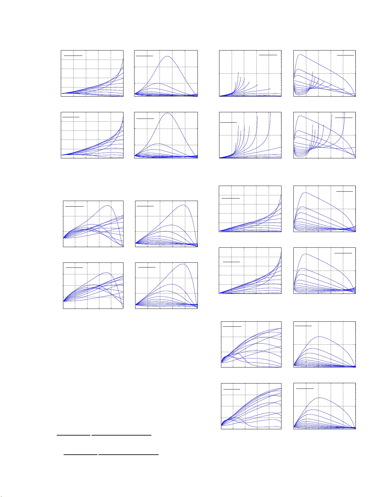
Accurate Estimators for Impro ving Min wise Hashing and b -Bit Min wise Hashing Ping Li Department of Statistical Science Cornell University Ithaca, NY 1 4853 pingli@cornell .edu Christian K¨ onig Microsoft Research Microsoft Co op ora tion Redmond, W A 98052 c hrisk o@microsoft.com Abstract Min wise 1 hashing is the standard technique in the context of se a rch and data bases for effi- ciently estimating set (e.g., hig h- dimensional 0/1 vector) similar ities. Recently , b-bit min- wise hashing w as propo sed whic h signifi- cantly improv es upon the original minwise hashing in practice b y sto ring only the low- est b bits of each hashed v alue, a s opp osed to using 64 bits. b-bit has hing is particularly effective in applications which mainly con- cern sets of hig h simila rities (e.g., the r esem- blanc e > 0 . 5 ). How ever, there are o ther im- po rtant applications in which not just pair s of high similar ities matter. F or example, many learning algorithms require all pairwise sim- ilarities and it is expected that only a small fraction of the pairs are similar. F urther- more, many applicatio ns care more a b o ut c ontainment (e.g., how muc h one ob ject is contained b y another o b ject) than the r esem- blanc e . In this paper, we show that the es- timators for minwise hashing and b-bit min- wise has hing used in the curr ent pra c tice can be systematica lly improv ed a nd the improv e- men ts are most significant for set pairs of low resemblance and high containmen t. 1 In tro duction Computing the size of set intersections is a fundamen- tal problem in infor mation re triev al, databases, and machine learning. F o r example, binary do cument vec- tors represented using w -s hing les ca n be vie wed either as vectors o f very high dimens io nality or as sets. The seminal w ork of minwise hashing [2, 4] is a standard to ol for efficiently co mputing r esemblanc es (Jacca rd similarity) among extremely high-dimensional (e.g., 2 64 ) binary vectors, which may be do cuments repre- sented by w -shingles ( w -grams , w contiguous words) 1 First draft in March, slightly mo dified in June, 2011. with w = 5 or 7 [2 , 4]. Min wise ha shing has been successfully applied to a very wide ra nge of real- world problems esp ecially in the con tex t o f sea rch; a partia l list includes [2, 4, 1, 13, 7, 27, 5, 29, 17, 1 0, 8, 14, 19, 25]. The r esemblanc e , R , is a widely used measure of sim- ilarity b etw een tw o sets. Consider t wo s ets S 1 , S 2 ⊆ Ω = { 0 , 1 , 2 , ..., D − 1 } , w he r e D , the size of the dic tio - nary , is often set to b e D = 2 64 in industry practice. Denote a = | S 1 ∩ S 2 | . R is defined a s R = | S 1 ∩ S 2 | | S 1 ∪ S 2 | = a f 1 + f 2 − a , f 1 = | S 1 | , f 2 = | S 2 | . Min wise hashing applies a random p e r mutation π : Ω → Ω on S 1 and S 2 . Base d on an elemen tar y proba- bilit y r esult: Pr (min( π ( S 1 )) = min( π ( S 2 ))) = | S 1 ∩ S 2 | | S 1 ∪ S 2 | = R, (1) one can store the sma llest elements under π , i.e., min( π ( S 1 )) and min( π ( S 2 )), and then rep eat the p er- m uta tion k times to estimate R . After k minwise inde- pendent per mut ations, π 1 , π 2 , ..., π k , one can estimate R without bias, as: ˆ R M = 1 k k X j =1 1 { min( π j ( S 1 )) = min( π j ( S 2 )) } , (2) V a r  ˆ R M  = 1 k R (1 − R ) . (3) The common practice is to stor e each hashed v alue, e.g., min( π ( S 1 )) and min ( π ( S 2 )), using 64 bits [12]. The storag e cos t (a nd consequently the computational cost) w ill be pro hibitive in large-sc a le applications [24]. It is well-understo o d in pra c tice tha t one c an reliably replace a p er mutation with a reas onable hashing func- tion; see the original min wis e hashing pap er [2] and the followup theor etical w o rk [3]. In o ther words, there is no need to stor e these k p ermutations. In this pa p er, we fir st obs e rve the standar d practice of min wis e hashing, i.e., using (2), can b e substantially improv ed for imp ortant scenarios . In fact, we will show that (2) is o ptimal only when the sets ar e of the same size, i.e., f 1 = f 2 , w hich is not to o co mmo n in practice. Figure 1 pr esents an example based on the websp am dataset (av ailable from the LibSVM site), which co n- tains 35 0000 do cuments represented using binary vec- tors of D = 16 million dimensions. Compar ed to the W e b sca le datase ts with billio ns of do cuments in 2 64 di- mensions, websp am is r elatively small and only use s 3- grams. Nev er theless, this example demonstrates that the set sizes (num b ers of no n-zeros), f i = | S i | , dis- tribute in a wide range. Therefore, when we co mpare t wo sets , s ay S 1 and S 2 , we exp ect the ratio f 1 /f 2 will often significantly deviate from 1. 0 1 2 3 4 5 x 10 4 0 1 2 3 4 x 10 4 Set sizes ( f ) Frequencies Figure 1 : Histo grams o f f i (n umber of non-zeros in the i -th data vector) in websp am dataset. Indeed, we computed the ratios f 1 /f 2 for all pairs in websp am . Without loss o f generality , w e alw ays as- sume f 1 ≥ f 2 . There are a ltogether 61 billion pairs with the mean f 1 /f 2 = 5.5 and the standar d deviation (std) = 9.5. Thus, w e exp ect that f 2 /f 1 = 0 . 2 ∼ 0 . 5 is c ommon and f 2 /f 1 < 0 . 1 is also fairly frequent . 1.1 The 3-Ce ll Multinomi al Problem The standard estimator (2) is based on a binomial dis- tribution. How ever, the pro blem really follows a 3 -cell m ultino mial distribution. Define z 1 = min( π ( S 1 )) a nd z 2 = min( π ( S 2 )). The three pr obabilities a re: P = = Pr ( z 1 = z 2 ) = a f 1 + f 2 − a = R, (4) P < = Pr ( z 1 < z 2 ) = f 1 − a f 1 + f 2 − a , (5) P > = Pr ( z 1 > z 2 ) = f 2 − a f 1 + f 2 − a (6) These pro babilities ar e easy to unders tand. F or exam- ple, for the ev ent { z 1 < z 2 } , the size of sample spac e is | S 1 ∪ S 2 | = f 1 + f 2 − a and the size of even t space is | S 1 − S 1 ∩ S 2 | = f 1 − a , and hence P < = f 1 − a f 1 + f 2 − a . W e will show tha t the estimator so lely based on P = (4) is optimal o nly when f 1 = f 2 . Assuming f 1 ≥ f 2 , then (5) should not be used for the estimation ta sk. The estimator base d on P > (6) is sup erio r to P = (6) when f 1 ≥ f 2 ≈ a . How ever, since w e do not kno w a in adv ance, we must combine all three pr obabilities to ensure accurate estimates. 1.2 The Measure of Co n tainme n t The r a tio T = a/f 2 (assuming f 1 ≥ f 2 ) is known as the c ont ainment . It is p oss ible that the resemblance R is sma ll but the co nt ainment T is larg e . Note that R = a f 1 + f 2 − a ≤ a/f 1 ≤ f 2 /f 1 . Thus, if, for exa mple, f 2 /f 1 ≤ 0 . 2, then R has to b e s mall, even when a ≈ f 2 (whic h corresp o nds to T ≈ 1). While the literature on minwise ha s hing has mainly fo cused on the estimation of set resemblance, accu- rate estimation o f set containmen t is also cr ucial to a num b er o f different applications. F or example, [9] uses b oth resemblance and cont a inment estimates of the w -gra ms cont a ined in text co lumns to characterize the s imilarity of database table co nten ts in a to ol that allows users to quickly understand database co nten t. In a similar c o ntext, [31] tests the (estimated) level of containmen t betw een the distinct v a lues contained in different (se ts of ) data base columns to automatically detect foreign key constra ints. [26] describ es the use of (estimated) s hingle co ntainmen t in the context of cluster-based compressio n schemes. In the context of ov erlay net works, [6 ] use s the estimated co ntainment (and resemblance) of the w o rking sets of p eers to co- ordinate betw een them, in turn reducing comm unica- tion cost and complex it y; b ecaus e only small mess ages should b e pa ssed for coo rdination, this e s timation has to b e based on sma ll synopses. The use of containmen t estimates in the c ontext of p eer- to-p eer netw orking is discussed in [15]. 1.3 b-Bit Mi n wis e Hashing The r ecent dev elo pment of b-bit minwise hash ing [22, 23, 20, 21] provides a solution to the (storag e and computational) problem o f minwise hashing by stor- ing only the low est b bits (instead of 64 bits) of ea ch hashed v alue for a small b. [22] prov ed that using only b = 1 bit p er hashed v a lue can achieve at lea st a 21.3-fold improv ement (in terms of storage) com- pared to using b = 64 bits if the target resemblance R > 0 . 5 . This is a very enc o uraging result whic h may lead to substantial improvemen t in applications like (near)duplicate detection of W e b pa ges [2 ]. On the other hand, when R is small, a s sho wn in [22, 21], one might have to increase b in order to achieve an adequate a c curacy without substantially increasing k , the num b e r of p ermutations. In fact, machine learning alg orithms like SVM r equire (essentially) all pairwise similarities and it is exp ected that most pairs are not too similar. Our concur rent work [21] attempts to combine linear SVM [18, 28, 11, 16, 3 0] with b-bit hashing; and our initial exp eriments suggest that b ≥ 4 (espe cially b = 8) is needed to achiev e go o d p erfor mance. In this pap er , we will provide estimators for both the standard minwise hashing and b-bit minwise hashing. 2 Estimators for Min wise Hashing Consider t wo sets S 1 , S 2 ∈ Ω = { 0 , 1 , 2 , ..., D − 1 } . f 1 = | S 1 | , f 2 = | S 2 | . a = | S 1 ∩ S 2 | . W e apply k r andom per mutations π j : Ω → Ω, and recor d the minimums z 1 ,j = min ( π j ( S 1 ), z 2 ,j = min ( π j ( S 2 ), j = 1 to k . W e will utilize the sizes o f thr e e disjoint sets: k = = |{ z 1 ,j = z 2 ,j , j = 1 , 2 , ..., k }| (7) k < = |{ z 1 ,j < z 2 ,j , j = 1 , 2 , ..., k }| (8) k > = |{ z 1 ,j > z 2 ,j , j = 1 , 2 , ..., k }| (9) Note that E ( k = ) = k P = , E ( k < ) = k P < , E ( k > ) = k P > , V ar ( k = ) = k P = (1 − P = ), etc. Thus, k = k , k < k , and k > k are unbiased estima to rs of P = (4), P < (5), and P > (6), resp ectively . F or the co nv enience of presentation, we estimate the in tersection a = ( f 1 + f 2 ) R 1+ R : ˆ a = = ( f 1 + f 2 ) k = /k 1 + k = /k = ( f 1 + f 2 ) k = k + k = (10) ˆ a < = f 1 − f 2 k < k − k < (11) ˆ a > = f 2 − f 1 k > k − k > , (12) which ar e a symptotically (for lar g e k ) un bia s ed esti- mators of a . The v a r iances ar e provided by Lemma 1. Lemma 1 V ar (ˆ a = ) = 1 k ( f 1 + f 2 − a ) 2 a ( f 1 + f 2 − 2 a ) ( f 1 + f 2 ) 2 + O  1 k 2  (13) V ar (ˆ a < ) = 1 k ( f 1 + f 2 − a ) 2 ( f 1 − a ) f 2 + O  1 k 2  (14) V ar (ˆ a > ) = 1 k ( f 1 + f 2 − a ) 2 ( f 2 − a ) f 1 + O  1 k 2  (15) Pr o of : The asymptotic varianc es c an b e c omput e d by the “delta metho d” V ar ( g ( x )) ≈ V ar ( x ) [ g ′ ( E ( x ))] 2 in a stra ightforwar d fashion. We skip the details.  2.1 The Maximum Lik eliho o d Estimator Lemma 1 sugg ests that the current standard estimator ˆ a = may b e severely less optimal when f 2 /f 1 deviates from 1. In fact, if we know f 1 > f 2 ≈ a (i.e., when the resemblance is s mall but the co nt a inment is lar ge), we will o btain goo d results b y using ˆ a > . The pro blem is that we do not kno w a in adv ance a nd hence we should resort to the maxim um likelihoo d estimator (MLE). Lemma 2 The MLE, denote d by ˆ a M LE , is the solu- tion t o the following e quation: k = f 1 + f 2 a − k < f 2 f 1 − a − k > f 1 f 2 − a = 0 (16) which is asymptotic al ly unbiase d with the vari anc e V ar (ˆ a M LE ) = 1 k ( f 1 + f 2 − a ) 2 f 1 + f 2 a + f 2 f 1 − a + f 1 f 2 − a + O  1 k 2  (17) Pr o of: The r esult fol lows fr om classic al multinomial estimation the ory. Se e Se ction 3.1.  2.2 Comparing MLE with Other E stimators Figure 2 compares the ratio s of the v ariances of estima- tors of a (only using the O  1 k  term of the v a riance). The top-left panel illustr ates that when f 2 /f 1 < 0 . 5 (whic h is common), the MLE ˆ a M LE can reduce the v ariance o f the standa r d estimator ˆ a = by a large fac- tor. When the target c o ntainmen t T = a f 2 approaches 1, the impr ov ement can be a s large a s 100-fold. The top-rig ht panel of Figure 2 sugg e sts that, if f 2 ≤ f 1 , then we should not use ˆ a < , b ec ause its v ar iance can be magnitudes larg er than the v a r iance of the MLE. The botto m- left panel confirms that if we know the containmen t is very la rge ( c lose to 1), then w e will do well by using ˆ a > which is simpler than the MLE. The problem is of cours e that w e do not know a in adv ance and hence we may still hav e to use the MLE. The bottom-r ight pa nel v e r ifies tha t ˆ a > is significantly better ˆ a < . 2.3 Exp erime n t F or the purp ose of verifying the theoretical impro ve- men ts, we use tw o pairs of sets corr esp onding to the o ccurrences of four common w o rds (“A – TEST” and “THIS – PERSON” ) in a c hunk of real world W eb crawl data. Eac h (w or d) set is a set of do cument (W eb page) IDs which contained tha t w ord at least once. F or “A – THE”, the resem blance = 0.05 24 and containmen t = 0.90 43. F or ‘THIS – PERSON”, the resemblance = 0.0903 and c ontainmen t = 0.8440 . Figure 3 presents the mean square errors (MSE) of the estimates using ˆ a = and ˆ a M LE . The results verify our theoretical predictions: 0 0.2 0.4 0.6 0.8 1 10 0 10 1 10 2 0.1 0.6 0.7 0.8 0.9 a / f 2 = 0.95 a / f 2 = 0.99 f 2 / f 1 Var ratios V a r ( ˆ a = ) V a r ( ˆ a M LE ) 0 0.2 0.4 0.6 0.8 1 10 0 10 2 10 4 10 6 0.1 0.2 0.95 a / f 2 = 0.99 f 2 / f 1 Var ratios V ar (ˆ a < ) V a r ( ˆ a M LE ) 0 0.2 0.4 0.6 0.8 1 1 5 10 15 20 a / f 2 = 0.1 a / f 2 = 0.2 0.3 0.4 0.5 0.6 0.7 0.99 f 2 / f 1 Var ratios V ar (ˆ a > ) V a r ( ˆ a M LE ) 0 0.2 0.4 0.6 0.8 1 10 0 10 2 10 4 10 6 0.1 0.7 0.8 0.9 0.95 a / f 2 = 0.99 f 2 / f 1 Var ratios V a r ( ˆ a < ) V a r ( ˆ a > ) Figure 2: V ar iance ratios (the low er the better). Ex - cept the b ottom-rig ht panel, w e compa re the other three estimators , ˆ a = , ˆ a < and ˆ a > , w ith the MLE ˆ a M LE . • F o r pairs of lo w resem blance and high co ntain- men t, the MLE ˆ a M LE provides significantly b et- ter (in these t wo cases, ab out an order of magni- tude b etter) r esults than the s ta ndard estimator ˆ a = . • The MLE is asymptotica lly un bia sed. The small bias at small k (which is co mmon for MLE in gen- eral) v anishes as k increa ses. • The theoretical v ar iances match the simulations. 50 100 100 0 10 4 10 5 10 6 10 7 Sample size k Mean square error (MSE) THIS − PERSON a = MLE Theoretical 50 100 1000 10 4 10 5 10 6 10 7 Sample size k Mean square error (MSE) A − TEST a = MLE Theoretical Figure 3: A sim ula tion study using tw o pairs of r e al- world v ector s (of low resemblance and high contain- men t) to verify (i) ˆ a M LE is significantly b etter than ˆ a = ; and (ii) the theoretical v ariances matc h the simu- lations and the bias of the MLE v anishes as k incr eases. 3 b -Bit Min wise Hashing b-Bit min wise hashing [22] stores eac h has he d v alue, e.g., z 1 = min( π ( S 1 )), z 2 = min( π ( S 2 )), using the low est b bits instead of 64 bits. In this sectio n, we will show that because the original b-bit min wis e hashing only used par t of the av ailable informa tion, it can b e substantially improved. W e fir st define: u 1 ,b = the nu m ber for med by the low est b bits of z 1 u 2 ,b = the nu m ber for med by the low est b bits of z 2 . [22] derived the pro bability form ula Pr ( u 1 ,b = u 2 ,b ) b y assuming D = | Ω | is large (whic h is virtually alwa ys satisfied in practice). W e will also need to derive P b, ( t,d ) = Pr ( u 1 ,b = t, u 2 ,b = d ) , t, d = 0 , 1 , 2 , ..., 2 b − 1 W e fo llow the conv ention in [22] b y defining r 1 = f 1 D , r 2 = f 2 D , s = a D (18) Instead of estimating a , we equiv alently estimate s in the context of b-bit hashing. Lemma 3 provides the probability formulas as the basic to ol. Lemma 3 Assume D is very lar ge. Pr ( u 1 ,b = t, u 2 ,b = d, t < d ) (19) = P < r 2 [1 − r 2 ] d − t − 1 1 − [1 − r 2 ] 2 b [1 − ( r 1 + r 2 − s )] t ( r 1 + r 2 − s ) 1 − [1 − ( r 1 + r 2 − s )] 2 b + P > r 1 [1 − r 1 ] t +2 b − d − 1 1 − [1 − r 1 ] 2 b [1 − ( r 1 + r 2 − s )] d ( r 1 + r 2 − s ) 1 − [1 − ( r 1 + r 2 − s )] 2 b Pr ( u 1 ,b = t, u 2 ,b = d, t > d ) (20) = P > r 1 [1 − r 1 ] t − d − 1 1 − [1 − r 1 ] 2 b [1 − ( r 1 + r 2 − s )] d ( r 1 + r 2 − s ) 1 − [1 − ( r 1 + r 2 − s )] 2 b + P < r 2 [1 − r 2 ] d +2 b − t − 1 1 − [1 − r 2 ] 2 b [1 − ( r 1 + r 2 − s )] t ( r 1 + r 2 − s ) 1 − [1 − ( r 1 + r 2 − s )] 2 b Pr ( u 1 ,b = t, u 2 ,b = t ) (21) = R + P < r 2 [1 − r 2 ] 2 b − 1 1 − [1 − r 2 ] 2 b + P > r 1 [1 − r 1 ] 2 b − 1 1 − [1 − r 1 ] 2 b ! × + [1 − ( r 1 + r 2 − s )] t ( r 1 + r 2 − s ) 1 − [1 − ( r 1 + r 2 − s )] 2 b Pr o of: Se e App endix A.  Therefore, we encounter a multinomial probability es- timation pr oblem with eac h cell probabilit y being a function of s . Note that the total num b er of cells, i.e., 2 b × 2 b , is la rge esp ecially when b is not sma ll. In additio n to P b, ( t,d ) , we also define the following three probability summarie s analogo us to P = , P < , and P > . P b, = = Pr ( u 1 ,b = u 2 ,b ) = 2 b − 1 X t =0 P b, ( t,t ) P b,<, = Pr ( u 1 ,b < u 2 ,b ) = 2 b − 1 X t = Pr ( u 1 ,b > u 2 ,b ) = 2 b − 1 X t>d P b, ( t,d ) Suppo se we conduct k permutations. W e define the observed counts, k b, ( t,d ) , k b, = , k b,< , and k b,> , which corres p o nd to P b, ( t,d ) , P b, = , P b,< , and P b,> , re s p e c- tively . Note that k = P t,d k b, ( t,d ) . [22] only used P b, = to estimate R (and hence also s ). W e exp ect to a chiev e substa nt ia l impr ov ement if we can take adv antage of the matrix of probabilities P b, ( t,d ) . Here, w e first review some basic statis tica l pro cedure for multinomial estimation and the classi- cal (asymptotic) v ariance a nalysis. 3.1 Review Classi cal Multinomial Estimatio n Consider a table with m cells, each of which is asso- ciated with a pro ba bility q i ( θ ), i = 1 , 2 , ..., m . Here we assume the probabilit y q i is parameterized b y θ (for example, the s in our problem), and the task is to estimate θ . Suppos e w e draw k i.i.d. samples and the n umber of obser v ations f r om th e i -th cell is k i , P m i =1 k i = k . The joint log-likelihoo d is prop ortiona l to l ( θ ) = m X i k i log q i ( θ ) . (22) The maximum likelihoo d estimator (MLE), which is optimal or a symptotically (for large k ) optimal in terms of the v ariance, is the solution ˆ θ M LE to the MLE equation l ′ ( θ ) = 0, i.e., l ′ ( θ ) = m X i =1 k i q ′ i ( θ ) q i ( θ ) = 0 , (23) solving which often requir es a numerical pro cedure. F or one - dimension problems as in our case, the n u- merical pro cedure is straightforw a rd. The estimation v ar iance of ˆ θ M LE is related to the Fisher Information I ( θ ) = − E ( l ′′ ( θ )): I ( θ ) = − E ( l ′′ ( θ )) = − m X i =1 E ( k i ) q ′′ i q i − [ q ′ i ] 2 q 2 i = − m X i =1 k q i q ′′ i q i − [ q ′ i ] 2 q 2 i = − k m X i =1 q ′′ i q i − [ q ′ i ] 2 q i (24) V ar  ˆ θ M LE  = 1 I ( θ ) + O  1 k 2  = 1 k 1 P m i =1 [ q ′ i ] 2 q i − q ′′ i + O  1 k 2  (25) F or b - bit hashing, since we ha ve 2 b × 2 b cells with probabilities P b, ( t,d ) , we can either use the full (entire) probably matr ix or v ario us reduced for ms by grouping (collapsing) cells (e.g ., P b, = , P b,< , and P b,> ) to ease the burden of numerically solving the MLE equation (23). 3.2 Fiv e Lev els of Es timators for s W e first in tr o duce the notation for the follo wing fiv e estimators of s : 1. ˆ s b,f denotes the full MLE solution by using all m = 2 b × 2 b cell proba bilities P b, ( t,d ) , t, d = 0 , 1 , 2 , ..., 2 b − 1 . This estimator will be most ac- curate and c o mputationally most intensiv e. 2. ˆ s b,do denotes the MLE solution b y using m = 2 b + 2 cells which include the 2 b diagonal probabilities P b, ( t,t ) , t = 0 , 1 , ..., 2 b − 1 a nd tw o summa r ies of the off-diag onals: P b,< = P t = P t>d P b, ( t,t ) . 3. ˆ s b,d denotes the MLE solution by using m = 2 b + 1 cells which include the 2 b diagonal pr obabilities P b, ( t,t ) , t = 0 , 1 , ..., 2 b − 1 and the sum o f the rest, i.e., P b,< + P b,> . 4. ˆ s b, 3 denotes the MLE solution by using m = 3 cells which include the sum of the diagonals and t wo sums of the off-diago nals, i.e., P b, = = P 2 b − 1 t =0 P b, ( t,t ) , P b,< , and P b,> . 5. ˆ s b, = denotes the MLE solution by using only m = 2 cells, i.e., P b, = and 1 − P b, = . This estimator requires no n umer ical so lutions and is the o ne used in the original b-bit minwise ha shing pap e r [22]. W e compare the asymptotic v ar iances of the other four estimators, ˆ s b,do , ˆ s b,d , ˆ s b, 3 , a nd ˆ s b, = , w ith the v ariance of the full MLE ˆ s b,f in Figures 4 to 12. W e consider b = 8 , 4 , 6, r 1 = 0 . 8 , 0 . 5 , 0 . 2 and th e full range s o f r 2 r 1 and s r 2 (whic h is the co ntainmen t). Note that the improv ement of this pap er compared to the previo us standard practice (i.e., ˆ s b, = ) is only reflected in the bo ttom-right pa nel of each figure. W e present other estimators in the hop e of finding one which is m uch simpler than the full MLE ˆ s b,f and still retains muc h of the improv ement. Our obs erv ations a re: • The full MLE ˆ s b,f , which us e s a matrix of 2 b × 2 b probabilities, can achiev e substant ial improv e- men ts (for example, 5- to 100-fold) compar ed to the standar d pr actice ˆ s b, = , esp ecially for cases of low resemblance and high containmen t. • Two other estimators, ˆ s b,do and ˆ s b, 3 usually per- form very w ell compar ed to the full MLE. ˆ s b,do uses 2 b + 2 ce lls and ˆ s b, 3 uses mere ly 3 c ells: the sum of the diagonals and the tw o sums of the off- diagonals . Therefore, we consider ˆ s b, 3 is likely to be pa rticularly useful in practice. 0 0.2 0.4 0.6 0.8 1 1 1.2 1.4 1.6 1.8 2 0.9 0.95 0.99 r 2 / r 1 Var ratios V a r ( ˆ s b,d o ) V ar ( ˆ s b,f ) b = 8, r 1 = 0.8 s / r 2 = 0.8 0.7 0.6 0.5 0.4 0.3 0 0.2 0.4 0.6 0.8 1 10 0 10 1 10 2 r 2 / r 1 Var ratios V a r ( ˆ s b,d ) V a r ( ˆ s b,f ) b = 8, r 1 = 0.8 s / r 2 = 0.99 0.95 0.9 0.8 0.6 0.1 0.7 0 0.2 0.4 0.6 0.8 1 1 1.5 2 2.5 3 0.9 0.95 0.99 r 2 / r 1 Var ratios V ar ( ˆ s b, 3 ) V a r ( ˆ s b,f ) b = 8, r 1 = 0.8 s / r 2 = 0.8 0.7 0.6 0.5 0.4 0.3 0 0.2 0.4 0.6 0.8 1 10 0 10 1 10 2 0.9 0.95 r 2 / r 1 Var ratios V a r ( ˆ s b, = ) V a r ( ˆ s b,f ) b = 8, r 1 = 0.8 s / r 2 = 0.99 0.8 0.6 0.1 0.7 Figure 4: Giv en a contingency table of s ize 2 b × 2 b , we hav e defined five different estimator s. W e compa re the theor etical v ariances of the other four estimator s, ˆ s b,do , ˆ s b,d , ˆ s b, 3 , a nd ˆ s b, = , with the v ariance o f the full MLE ˆ s b,f . The b ottom-r ight panel measures the r eal improv ement of this pap er compared to the previo us standard practice (i.e., ˆ s b, = ). In this case, t he v ar i- ance ra tios o f about 10 to 100 a re very substa ntial. The other thr e e panels are for testing whether simpler estimators can still achiev e substantial improvemen ts. F or ex ample, both ˆ s b,do and ˆ s b, 3 (the left t wo panels) only magnify the v ariance of the full MLE by small fac- tors compared to ˆ s b, = , and hence they might b e go o d estimators in lieu of the quite so phisticated full MLE solution. In this fig ure, we consider b = 8 and r 1 = 0.8 . Note that s/r 2 is the c ontainmen t. The resemblance is upp er bounded by r 2 /r 1 . . 0 0.2 0.4 0.6 0.8 1 1 1.2 1.4 1.6 1.8 s / r 2 = 0.2 0.3 0.4 0.5 0.6 0.7 0.8 0.9 0.95 r 2 / r 1 Var ratios V a r ( ˆ s b,d o ) V ar ( ˆ s b,f ) b = 8, r 1 = 0.5 0.1 0 0.2 0.4 0.6 0.8 1 10 0 10 1 10 2 r 2 / r 1 Var ratios V a r ( ˆ s b,d ) V a r ( ˆ s b,f ) b = 8, r 1 = 0.5 s / r 2 = 0.99 0.95 0.9 0.8 0.7 0.6 0.1 0 0.2 0.4 0.6 0.8 1 1 1.2 1.4 1.6 1.8 0.3 0.4 0.5 0.6 0.7 0.8 0.9 0.95 0.99 r 2 / r 1 Var ratios V ar ( ˆ s b, 3 ) V a r ( ˆ s b,f ) b = 8, r 1 = 0.5 s / r 2 = 0.2 0.1 0 0.2 0.4 0.8 1 10 0 10 1 10 2 r 2 / r 1 Var ratios V a r ( ˆ s b, = ) V a r ( ˆ s b,f ) b = 8, r 1 = 0.5 s / r 2 = 0.99 0.95 0.9 0.8 0.7 0.6 0.1 Figure 5 : V a r iance r atios for b = 8 and r 1 = 0 . 5. See the caption of Figure 4 for more details. 0 0.2 0.4 0.6 0.8 1 1 1.05 1.1 1.15 1.2 0.1 0.2 s / r 2 = 0.4 0.5 0.6 0.7 0.8 0.9 0.95 0.99 r 2 / r 1 Var ratios V a r ( ˆ s b,d o ) V ar ( ˆ s b,f ) b = 8, r 1 = 0.2 0 0.2 0.4 0.6 0.8 1 10 0 10 1 10 2 r 2 / r 1 Var ratios V a r ( ˆ s b,d ) V a r ( ˆ s b,f ) b = 8, r 1 = 0.2 s / r 2 = 0.99 0.95 0.9 0.8 0.7 0.1 0 0.2 0.4 0.6 0.8 1 1 1.05 1.1 1.15 1.2 0.1 0 .2 0.3 s / r 2 = 0.5 0.7 0.8 0.9 0.95 s / r 2 = 0.99 r 2 / r 1 Var ratios V ar ( ˆ s b, 3 ) V a r ( ˆ s b,f ) b = 8, r 1 = 0.2 0 0.2 0.4 0.6 0.8 1 10 0 10 1 10 2 0.1 0.7 0.8 0.9 0.95 r 2 / r 1 Var ratios V a r ( ˆ s b, = ) V a r ( ˆ s b,f ) b = 8, r 1 = 0.2 s / r 2 = 0.99 Figure 6: V ar ia nce ratios for b = 8 and r 1 = 0 . 2. 0 0.2 0.4 0.6 0.8 1 10 0 10 1 10 2 0.1 0.3 0.4 0.5 0.6 0.7 0.8 r 2 / r 1 Var ratios V a r ( ˆ s b,d o ) V ar ( ˆ s b,f ) b = 4, r 1 = 0.8 s / r 2 = 0.2 0 0.2 0.4 0.6 0.8 1 10 0 10 1 10 2 0.1 0.2 0.3 0.4 0.5 0.6 0.7 r 2 / r 1 Var ratios V a r ( ˆ s b,d ) V a r ( ˆ s b,f ) b = 4, r 1 = 0.8 s / r 2 = 0.99 0.95 0.9 0.8 0 0.2 0.4 0.6 0.8 1 10 0 10 1 10 2 0.1 0.2 0.3 0.4 0.5 0.8 0.9 r 2 / r 1 Var ratios V ar ( ˆ s b, 3 ) V a r ( ˆ s b,f ) b = 4, r 1 = 0.8 s / r 2 = 0.7 0.6 0 0.2 0.4 0.6 0.8 1 10 0 10 1 10 2 0.1 0.2 0.3 0.4 0.5 0.6 s / r 2 = 0.7 0.8 0.9 0.95 0.99 r 2 / r 1 Var ratios V a r ( ˆ s b, = ) V a r ( ˆ s b,f ) b = 4, r 1 = 0.8 Figure 7: V ar ia nce ratios for b = 4 and r 1 = 0 . 8. 0 0.2 0.4 0.6 0.8 1 1 1.2 1.4 1.6 1.8 2 0.2 0.3 0.4 0.5 0.6 0.7 0.8 0.9 r 2 / r 1 Var ratios V a r ( ˆ s b,d o ) V ar ( ˆ s b,f ) b = 4, r 1 = 0.5 s / r 2 = 0.1 0 0.2 0.4 0.6 0.8 1 1 5 10 15 r 2 / r 1 Var ratios V a r ( ˆ s b,d ) V a r ( ˆ s b,f ) b = 4, r 1 = 0.5 s / r 2 = 0.99 0.95 0.9 0.8 0 0.2 0.4 0.6 0.8 1 1 1.2 1.4 1.6 1.8 2 0.2 0.3 0.4 0.5 0.6 0.7 0.8 0.9 0.95 0.99 r 2 / r 1 Var ratios V ar ( ˆ s b, 3 ) V a r ( ˆ s b,f ) b = 4, r 1 = 0.5 s / r 2 = 0.1 0 0.2 0.4 0.6 0.8 1 1 5 10 15 r 2 / r 1 Var ratios V a r ( ˆ s b, = ) V a r ( ˆ s b,f ) b = 4, r 1 = 0.5 s / r 2 = 0.99 0.95 0.9 0.8 Figure 8: V ar ia nce ratios for b = 4 and r 1 = 0 . 5. 0 0.2 0.4 0.6 0.8 1 1 1.05 1.1 1.15 0.2 0.6 0.7 0.8 0.9 0.95 r 2 / r 1 Var ratios V a r ( ˆ s b,d o ) V ar ( ˆ s b,f ) 0.1 b = 4, r 1 = 0.2 s / r 2 = 0.99 0 0.2 0.4 0.6 0.8 1 1 1.5 2 2.5 r 2 / r 1 Var ratios V a r ( ˆ s b,d ) V a r ( ˆ s b,f ) b = 4, r 1 = 0.2 s / r 2 = 0.99 0.95 0.9 0.8 0.7 0.1 0 0.2 0.4 0.6 0.8 1 1 1.05 1.1 1.15 1.2 0.3 0.9 r 2 / r 1 Var ratios V ar ( ˆ s b, 3 ) V a r ( ˆ s b,f ) b = 4, r 1 = 0.2 s / r 2 = 0.99 0.95 0.1 0.2 0 0.2 0.4 0.6 0.8 1 1 1.5 2 2.5 r 2 / r 1 Var ratios V a r ( ˆ s b, = ) V a r ( ˆ s b,f ) b = 4, r 1 = 0.2 s / r 2 = 0.99 0.95 0.9 0.8 0.7 0.1 Figure 9: V ar ia nce ratios for b = 4 and r 1 = 0 . 2. Our analys is has demons trated that the m uch simpler estimator ˆ s b, 3 , which only us e s 3 cells, is often remar k- ably accur ate. W e expect it will be used in prac tice. ˆ s b, 3 inv olves three summary pro babilities: P b, = , P b,< , and P b,> . F or efficien t e stimation, we will need to use more compact presentations instead of the double summation for ms . Since w e a lready know P b, = as de- rived in [22], we only need to derive P b,< and then P b,> follows by symmetry . After some algebra, w e o btain P b,< = Pr ( u 1 ,b < u 2 ,b ) = 2 b − 1 X t j ) = r 1 ( r 2 − s ) [ 1 − r 1 ] i − j − 1 [1 − ( r 1 + r 2 − s )] j (28) W e will also need to derive Pr ( z 1 = i, z 2 = i ). The exact expression is given by Pr ( z 1 = i, z 2 = i ) =  D − i − 1 a − 1  D − i − a f 1 − a  D − i − f 1 f 2 − a   D a  D − a f 1 − a  D − f 1 f 2 − a  = a ( D − i − 1)!( D − f 1 − f 2 + a )! D !( D − f 1 − f 2 + a − i )! = a D Q i − 1 t =0 D − f 1 − f 2 + a − t Q i − 1 t =0 D − 1 − t F or conv enienc e , we introduce the following notation: r 1 = f 1 D , r 2 = f 2 D , s = a D . Also, w e assume D is lar ge (which is vir tually a lwa ys satisfied in pra ctice). W e ca n obtain a r easonable ap- proximation (analog ous to the P ossion appr oximation of binomial): Pr ( z 1 = i, z 2 = i ) = s [1 − ( r 1 + r 2 − s )] i T o v e r ify this, a s expec ted, Pr ( z 1 = z 2 ) = X i Pr ( z 1 = i, z 2 = i ) = X i s [1 − ( r 1 + r 2 − s )] i = s r 1 + r 2 − s = R Now we hav e to ols to co mpute Pr ( u 1 ,b = t, u 2 ,b = d ), where t, d ∈ { 0 , 1 , 2 , 3 , ..., 2 b − 1 } . Pr ( u 1 ,b = t, u 2 ,b = d, t < d ) = Pr ( z 1 = t, t + 2 b , t + 2 × 2 b , t + 3 × 2 b , ..., z 2 = d, d + 2 b , d + 2 × 2 b , d + 3 × 2 b , ... ) Pr  z 1 = t, z 2 = d, d + 2 b , d + 2 × 2 b , d + 3 × 2 b , ...,  = X j =0 Pr  z 1 = t, z 2 = d + j × 2 b , ...,  = X j =0 r 2 ( r 1 − s ) [ 1 − r 2 ] d + j × 2 b − t − 1 [1 − ( r 1 + r 2 − s )] t = r 2 ( r 1 − s ) [1 − r 2 ] d − t − 1 1 − [ 1 − r 2 ] 2 b [1 − ( r 1 + r 2 − s )] t Pr  z 1 = t + 2 b , z 2 = d + 2 b , d + 2 × 2 b , d + 3 × 2 b , ...,  = X j =1 Pr  z 1 = t + 2 b , z 2 = d + j × 2 b , ...,  = X j =1 r 2 ( r 1 − s ) [1 − r 2 ] d + j × 2 b − t − 2 b − 1 [1 − ( r 1 + r 2 − s )] t +2 b = r 2 ( r 1 − s ) [1 − r 2 ] d − t − 1 1 − [1 − r 2 ] 2 b [1 − ( r 1 + r 2 − s )] t +2 b Pr ( u 1 ,b = t, u 2 ,b = d, t < d, z 1 < z 2 ) = X i =0 r 2 ( r 1 − s ) [1 − r 2 ] d − t − 1 1 − [1 − r 2 ] 2 b [1 − ( r 1 + r 2 − s )] t + i × 2 b = r 2 ( r 1 − s ) [1 − r 2 ] d − t − 1 1 − [1 − r 2 ] 2 b [1 − ( r 1 + r 2 − s )] t 1 − [1 − ( r 1 + r 2 − s )] 2 b Next, w e study Pr ( u 1 ,b = t, u 2 ,b = d, t < d, z 1 > z 2 ) Pr  z 1 = d, ..., z 2 = t + 2 b , t + 2 × 2 b , t + 3 × 2 b , ..., t < d  = X j =1 r 2 ( r 1 − s ) [1 − r 2 ] t + j × 2 b − d − 1 [1 − ( r 1 + r 2 − s )] d = r 2 ( r 1 − s ) [1 − r 2 ] t +2 b − d − 1 1 − [1 − r 2 ] 2 b [1 − ( r 1 + r 2 − s )] d Pr  z 1 = d + 2 b , ..., z 2 = t + 2 × 2 b , t + 3 × 2 b , ..., t < d  = X j =2 r 2 ( r 1 − s ) [1 − r 2 ] t + j × 2 b − d − 2 b − 1 [1 − ( r 1 + r 2 − s )] d +2 b = r 2 ( r 1 − s ) [1 − r 2 ] t +2 b − d − 1 1 − [1 − r 2 ] 2 b [1 − ( r 1 + r 2 − s )] d +2 b Pr ( z 1 = d, d + 2 b , d + 2 × 2 b ..., z 2 = t, t + 2 b , t + 2 × 2 b , ..., t < d, z 1 < z 2 ) = X i =0 r 2 ( r 1 − s ) [1 − r 2 ] t +2 b − d − 1 1 − [1 − r 2 ] 2 b [1 − ( r 1 + r 2 − s )] d + i × 2 b = r 2 ( r 1 − s ) [1 − r 2 ] t +2 b − d − 1 1 − [ 1 − r 2 ] 2 b [1 − ( r 1 + r 2 − s )] d 1 − [1 − ( r 1 + r 2 − s )] 2 b By symmetry Pr ( z 1 = t, t + 2 b , t + 2 × 2 b , ..., z 2 = d, d + 2 b , d + 2 × 2 b ..., t < d, z 1 > z 2 ) = r 1 ( r 2 − s ) [1 − r 1 ] t +2 b − d − 1 1 − [1 − r 1 ] 2 b [1 − ( r 1 + r 2 − s )] d 1 − [1 − ( r 1 + r 2 − s )] 2 b Combining the results yields Pr ( u 1 ,b = t, u 2 ,b = d, t < d ) = r 2 ( r 1 − s ) [1 − r 2 ] d − t − 1 1 − [1 − r 2 ] 2 b [1 − ( r 1 + r 2 − s )] t 1 − [1 − ( r 1 + r 2 − s )] 2 b + r 1 ( r 2 − s ) [1 − r 1 ] t +2 b − d − 1 1 − [ 1 − r 1 ] 2 b [1 − ( r 1 + r 2 − s )] d 1 − [1 − ( r 1 + r 2 − s )] 2 b Pr ( u 1 ,b = t, u 2 ,b = d, t > d ) = Pr ( u 2 ,b = d, u 1 ,b = t, d < t ) = r 1 ( r 2 − s ) [1 − r 1 ] t − d − 1 1 − [1 − r 1 ] 2 b [1 − ( r 1 + r 2 − s )] d 1 − [1 − ( r 1 + r 2 − s )] 2 b + r 2 ( r 1 − s ) [1 − r 2 ] d +2 b − t − 1 1 − [ 1 − r 2 ] 2 b [1 − ( r 1 + r 2 − s )] t 1 − [1 − ( r 1 + r 2 − s )] 2 b Now, we need to compute Pr ( u 1 ,b = t, u 2 ,b = t ): Pr ( u 1 ,b = t, u 2 ,b = t ) = X i =0 X j =0 Pr  z 1 = t + i × 2 b , z 2 = t + j × 2 b  Pr ( u 1 ,b = t, u 2 ,b = t ) = Pr ( u 1 ,b = t, u 2 ,b = t, z 1 = z 2 ) + Pr ( u 1 ,b = t, u 2 ,b = t, z 1 6 = z 2 ) Pr ( u 1 ,b = t, u 2 ,b = t, z 1 = z 2 ) = X i =0 Pr  z 1 = z 2 = t + i × 2 b , ...  = X i =0 s [ 1 − ( r 1 + r 2 − s )] t + i × 2 b = s [ 1 − ( r 1 + r 2 − s )] t 1 − [1 − ( r 1 + r 2 − s )] 2 b Pr ( u 1 ,b = t, u 2 ,b = t, z 1 < z 2 ) = X i =0 X j = i +1 Pr  z 1 = t + i × 2 b , z 2 = t + j × 2 b  = X i =0 X j = i +1 r 2 ( r 1 − s ) [1 − r 2 ] ( j − i ) × 2 b − 1 [1 − ( r 1 + r 2 − s )] t + i × 2 b = X i =0 r 2 ( r 1 − s ) [1 − r 2 ] 2 b − 1 1 − [ 1 − r 2 ] 2 b [1 − ( r 1 + r 2 − s )] t + i × 2 b = r 2 ( r 1 − s ) [1 − r 2 ] 2 b − 1 1 − [1 − r 2 ] 2 b [1 − ( r 1 + r 2 − s )] t 1 − [ 1 − ( r 1 + r 2 − s )] 2 b Pr ( u 1 ,b = t, u 2 ,b = t, z 1 > z 2 ) = r 1 ( r 2 − s ) [1 − r 1 ] 2 b − 1 1 − [ 1 − r 1 ] 2 b [1 − ( r 1 + r 2 − s )] t 1 − [1 − ( r 1 + r 2 − s )] 2 b Combining the results yields Pr ( u 1 ,b = t, u 2 ,b = t ) = s [1 − ( r 1 + r 2 − s )] t 1 − [1 − ( r 1 + r 2 − s )] 2 b + r 2 ( r 1 − s ) [1 − r 2 ] 2 b − 1 1 − [1 − r 2 ] 2 b [1 − ( r 1 + r 2 − s )] t 1 − [1 − ( r 1 + r 2 − s )] 2 b + r 1 ( r 2 − s ) [1 − r 1 ] 2 b − 1 1 − [1 − r 1 ] 2 b [1 − ( r 1 + r 2 − s )] t 1 − [1 − ( r 1 + r 2 − s )] 2 b Finally , we re-write the pr obabilities in terms of R = P = , P < , and P > whenever po ssible: Pr ( u 1 ,b = t, u 2 ,b = d, t < d ) = P < r 2 [1 − r 2 ] d − t − 1 1 − [1 − r 2 ] 2 b [1 − ( r 1 + r 2 − s )] t ( r 1 + r 2 − s ) 1 − [1 − ( r 1 + r 2 − s )] 2 b + P > r 1 [1 − r 1 ] t +2 b − d − 1 1 − [ 1 − r 1 ] 2 b [1 − ( r 1 + r 2 − s )] d ( r 1 + r 2 − s ) 1 − [1 − ( r 1 + r 2 − s )] 2 b Pr ( u 1 ,b = t, u 2 ,b = d, t > d ) = P > r 1 [1 − r 1 ] t − d − 1 1 − [1 − r 1 ] 2 b [1 − ( r 1 + r 2 − s )] d ( r 1 + r 2 − s ) 1 − [ 1 − ( r 1 + r 2 − s )] 2 b + P < r 2 [1 − r 2 ] d +2 b − t − 1 1 − [ 1 − r 2 ] 2 b [1 − ( r 1 + r 2 − s )] t ( r 1 + r 2 − s ) 1 − [1 − ( r 1 + r 2 − s )] 2 b Pr ( u 1 ,b = t, u 2 ,b = t ) = R + P < r 2 [1 − r 2 ] 2 b − 1 1 − [1 − r 2 ] 2 b + P > r 1 [1 − r 1 ] 2 b − 1 1 − [1 − r 1 ] 2 b ! × + [1 − ( r 1 + r 2 − s )] t ( r 1 + r 2 − s ) 1 − [ 1 − ( r 1 + r 2 − s )] 2 b References [1] Mic h ael Bend ersky and W. Bruce Croft. Finding text reuse on the w eb . In WSDM , p ages 26 2–271, Barcelona, Spain, 2009. [2] Andrei Z. Broder. O n the resemblance and conta in- ment of do cuments. In the Compr ession and Complex- ity of Se quenc es , pages 21–29, Positano, Italy , 1997. [3] Andrei Z. Bro der, Moses Charik ar, Alan M. F rieze, and Mic hael Mitzenmacher. Min-wise indep endent p ermutations (ex t ended abstract). In STOC , pages 327–336 , Dallas , TX, 1998. [4] Andrei Z. Bro der, Steven C. Glassman, Mark S. Man- asse, and Geoffrey Zwei g. S yntactic clustering of the w eb. In WW W , pages 1157 – 1166, S anta Clara, CA, 1997. [5] Gregory Buehrer and Ku mar Chellapilla. A scalable pattern mining approach to web graph compression with communities. In WSDM , pages 95–106, Stanford, CA, 2008. [6] John Byers, Jeffrey Considine, Michael Mitzen- mac h er, and Stanisla v Rost. Informed Conten t Deliv- ery across Adaptive Overla y N etw orks. In SIGCOMM , pages 47–60, 2002. [7] Ludmila Cherk asov a, Kav e Eshghi, Charles B. Morrey I I I, Joseph T ucek, and Alistair C. V eitch. A pplying syntactic similarit y algori t h ms for enterprise informa- tion managemen t. In KDD , pages 1087–1096, Paris, F rance, 2009. [8] Fla v io Chierichetti, Ra v i Kumar, Silvio Lattanzi, Mic hael Mitzenmac her, Alessandro Panconesi, an d Prabhak ar Ragha van. On compressing so cial n et- w orks. In KDD , pages 219–228, Paris, F rance, 2009. [9] T. Dasu, T. Johnson, S. Muthukrishnan, and V. S hk ap enyuk. Mining database stru cture; or, ho w to b u ild a data q uality brow ser. In SIGMOD , pages 240–251 , Madison, WI, 2002. [10] Y on D ou risb oure, Filippo Geraci, and Marco Pelle- grini. Extraction and classification of dense implicit comm u nities in the web graph. ACM T r ans. W eb , 3(2):1–36, 2009. [11] Rong-En F an, Kai-W ei Chang, Cho-Jui Hsieh, Xiang- Rui W ang, and Chih-Jen Lin. Liblinear: A library for large linear classificatio n . Journal of Machine L e arn- ing Re se ar ch , 9:1871–18 74, 2008. [12] Dennis F etterly , Mark Manasse, Marc N a jork, and Janet L. Wiener. A large-scale study of th e evol u tion of web pages. In WWW , pages 669–67 8, Budap est, Hungary , 2003. [13] George F orman, Kav e Eshghi, and Jaap Suermondt. Efficien t d etection of large-scale red undancy in enter- prise file systems. SIGOPS Op er. Syst. R ev. , 43(1):84 – 91, 2009. [14] Sreeniv as Gollapudi and Aneesh S harma. A n ax- iomatic approach for result diversification. In WWW , pages 381–390 , Madrid, Spain, 2009. [15] Systems A bhishek Gupta, A bhishek Gupta, Di- vyak an t Agra wal, and Amr El Abbadi. Approximate Range Selection Queries in Peer-to-Peer. In In CIDR , 2002. [16] Cho-Jui Hsieh, Kai-W ei Chang, Chih-Jen Lin, S. Sathiya Keerthi, and S. Sundarara jan. A d ual co- ordinate descent metho d for large-scale linear svm. In Pr o c e e dings of the 25th international c onfer enc e on Machine le arning , ICML, pages 408–415, 2008. [17] Nitin Jindal and Bing Liu. Opinion spam and analysis. In WSDM , pages 219–230, Palo Alto, California, U S A, 2008. [18] Thorsten Joachims. T raining l in ear svms in linear time. In KDD , p ages 217–226, Pittsburgh, P A, 2006. [19] Konstantinos Kalpakis and S hilang T ang. Collabora- tive data gathering in wireless sensor n etw orks using measuremen t co-occurrence. Computer Communi c a- tions , 31(10):1979–1 992, 2008. [20] Ping Li and Arnd Christian K¨ onig. Theory and ap- plications b-b it minwise hashing. In Commun. A CM , 2011. [21] Ping Li, A nshumali Sh rivas tav a, Josh u a Mo ore, and Arnd Christian K¨ onig. Hashing algorithms for large- scale learning. T echnical rep ort. [22] Ping Li and Arnd Christian K¨ onig. b-b it minwis e hashing. I n WWW , pages 671–680, Raleigh, N C, 2010. [23] Ping Li, A rnd Christian K ¨ onig, and W enhao Gui. b- bit minw ise hashing for estimating three-wa y similar- ities. In NI PS , V ancouv er, BC, 2010. [24] Gurmeet Singh Manku, Arv ind Jain, and An ish Das Sarma. Detecting Near-Duplicates for Web-Craw ling. In WWW , Banff, A lb erta, Canada, 2007. [25] Marc N a jork, Sreeniv as Gollapudi, and Rina P ani- grah y . Less is more: sampling the n eighborhoo d graph makes salsa better and faster. In WSDM , pages 242– 251, Barcelona, Sp ain, 2009. [26] Zan Ou yang, Nasir D. Memon, T orsten Suel, and Dimitre T rend afilo v . Cluster-Based Delta Compres- sion of a Collecti on of Files. In WI SE , p ages 257–268, 2002. [27] Sandeep Pandey , Andrei Bro der, Flavio Chieric hetti, V anja Josifo vski, Ravi Kumar, and Sergei V assilvit- skii. Nearest-neighbor caching for conten t-match ap- plications. In W WW , pages 441–450, Madrid, Spain, 2009. [28] Shai Shalev-Shw artz, Y oram Singer, and Nathan Sre- bro. Pega sos: Primal estimated sub- gradien t solver for svm. In ICML , pages 807–814, Corv alis, Oregon, 2007. [29] T anguy Urvo y , Emmanuel Chauveau, Pasca l Filo che, and Thomas Lav ergne. T racking w eb spam with html style similarities. ACM T r ans. W eb , 2(1):1–28, 2008. [30] Hsiang-F u Y u , Cho-Jui Hsieh, Kai-W ei Chang, and Chih-Jen Lin. Large linear class ification when data cannot fit in memory . In KDD , p ages 833–842, 2010. [31] Meih u i Zhang, Marios Hadjielef th eriou, Beng Chin Ooi, Cecili a M. Procopiuc, and Divesh Sriv asta va . On Multi-column F oreign Key D isco very . Pr o c. V LDB Endow. , 3:805–814 , Septem b er 2010.