Algorithmic and Complexity Results for Cutting Planes Derived from Maximal Lattice-Free Convex Sets

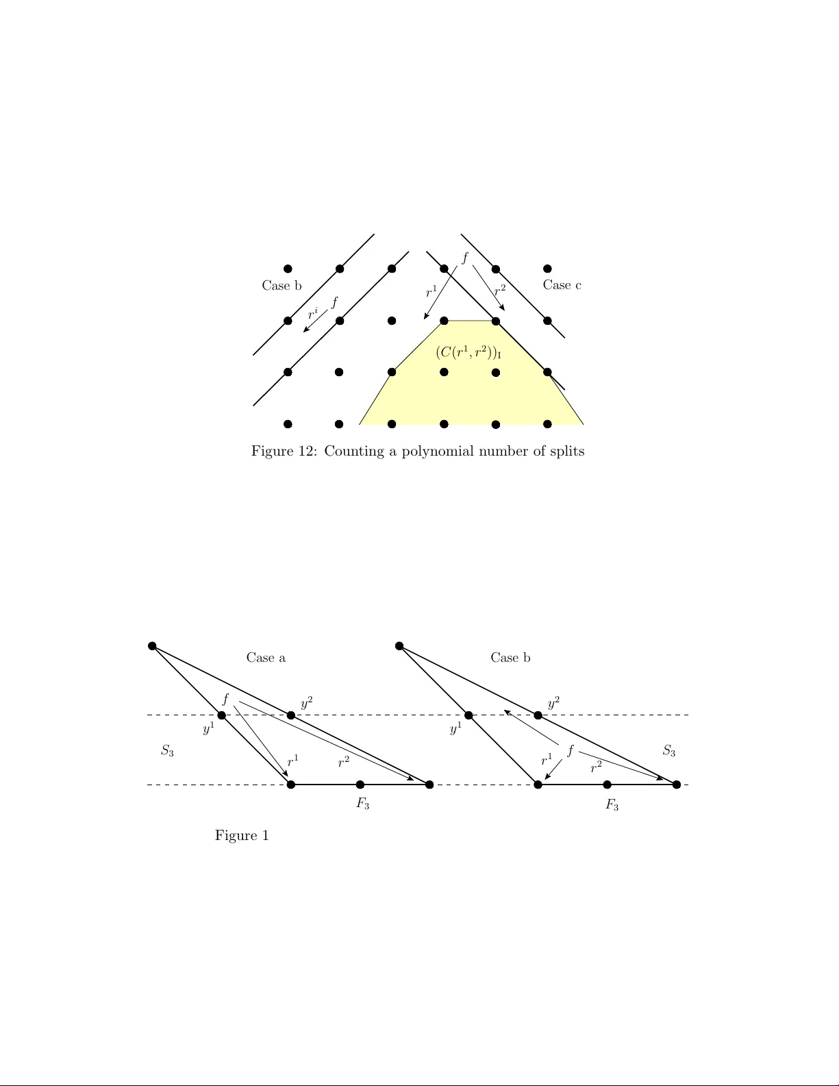
Algorithmic and Complexit y Results for Cutting Planes Deriv ed from Maximal Lattice-F ree Con v ex Sets Amitabh Basu ∗ Rob ert Hildebrand † Matthias K¨ opp e ‡ July 25, 2011 § Abstract W e study a mixed in teger linear program with m integer v ariables and k non- negativ e con tinuous v ariables in the form of the relaxation of the corner p olyhedron that w as introduced b y Andersen, Louveaux, W eisman tel and W olsey [ Ine qualities fr om two r ows of a simplex table au , Pro c. IPCO 2007, LNCS, v ol. 4513, Springer, pp. 1–15]. W e describe the facets of this mixed in teger linear program via the extreme p oints of a well-deﬁned p olyhedron. W e then utilize this description to give p olynomial time algorithms to derive v alid inequalities with optimal l p norm for arbitrary , but ﬁxed m . F or the case of m = 2, we giv e a reﬁnement and a new pro of of a characterization of the facets by Cornu ´ ejols and Margot [ On the fac ets of mixe d inte ger pr o gr ams with two inte ger variables and two c onstr aints , Math. Programming 120 (2009), 429–456]. The k ey p oint of our approach is that the conditions are m uch more explicit and can b e tested in a more direct manner, removing the need for a reduction algorithm. These results allow us to sho w that the relaxed corner p olyhedron has only p olynomially many facets. 1 In tro duction The in teger programming comm unity has recently fo cused on developing a unifying the- ory for cutting planes. This has in volv ed applying tools from conv ex analysis and the geometry of n umbers to combine the ideas b ehind Gomory’s corner p olyhedron [13] and Balas’ in tersection cuts [2] into one uniform framew ork. It is fair to say that this recent line of research was started by the seminal paper by Andersen, Louveaux, W eismantel and W olsey [1], which to ok a fresh lo ok at the w ork done by Gomory and Johnson in the 1960’s. W e refer the reader to [8] for a survey of these results. It can b e argued that the theoretical research has tended to emphasize the structural asp ects of these cutting planes and the algorithmic asp ects hav e not b een developed as ∗ Dept. of Mathematics, Universit y of California, Davis, abasu@math.ucdavis.edu † Dept. of Mathematics, Universit y of California, Davis, rhildebrand@math.ucdavis.edu ‡ Dept. of Mathematics, Universit y of California, Davis, mkoeppe@math.ucdavis.edu § Revision: 201 − Date: 2011-07-25 12:55:40 -0700 (Mon, 25 Jul 2011) 1 in tensively . Our goal in this pap er is to derive structural results which, we hop e, will b e useful from an algorithm design p ersp ectiv e. Hence, our emphasis is on deriving p oly- nomialit y results ab out the structure of these cutting planes. W e also provide concrete p olynomial time algorithms for generating the “b est” or “deep est” cuts, according to some standard criteria. T o this end, we study the follo wing system, introduced by Andersen et al. [1] and Borozan and Corn u´ ejols [7]. x = f + k X j =1 r j s j , x ∈ Z m , s j ≥ 0 for all j = 1 , . . . , k. (1) W e will assume that the data is rational, i.e., f ∈ Q m and r j ∈ Q m for all j ∈ { 1 , . . . , k } . This mo del app ears as a natural relaxation of Gomory’s corner p olyhe- dron [13]. As mentioned ab ov e, this mo del has receiv ed signiﬁcan t attention in recent y ears for developing the theory b ehind cutting planes derived from multiple rows of the optimal simplex tableaux. Note that to describ e the solutions of (1), one only needs to record the v alues of the s j v ariables. W e use R f = R f ( r 1 , . . . , r k ) to denote the set of all p oin ts s suc h that (1) is satisﬁed. It is w ell-kno wn that all v alid inequalities for con v( R f ), where conv denotes the conv ex hull, can b e derived using the Mink owski functional of maximal lattice-free conv ex sets. W e state this formally in Theorem 2.2 b elo w. In this pap er we giv e algorithms and theorems ab out the facet structure of conv( R f ), which are exp ected to b e useful for generating strong cutting planes for general mixed integer linear programs. Motiv ation and Results. It is well-kno wn that the in teger hull con v( R f ) is a p olyhe- dron of the blo cking typ e . In Section 3, we ﬁrst describ e the so-called blo cking p olyhe dr on for conv( R f ). This is the con vex set of all v alid inequalities for c on v( R f ). F or a de- tailed account of blocking polyhedra and the “p olar” set of the v alid inequalities for such p olyhedra, see Chapter 9 in [19]. The main result of Section 3 gives an explicit descrip- tion of the blo c king p olyhedron of conv( R f ) using a p olynomial num b er of inequalities (Theorem 3.3). This implies that all facets of con v ( R f ) can b e obtained by en umerat- ing the extreme p oints of a p olyhedron with a p olynomial num ber of facets in the dual space. This result has the same ﬂav or as Gomory’s result for describing all facets of the corner p olyhedron implicitly via the extreme p oints of a well-deﬁned p olyhedron (see Theorem 18 in [13]). W e next exploit this to provide eﬃcien t algorithms for ﬁnding the optimal v alid inequalit y according to certain norms of the co eﬃcient v ector. More precisely , let k v k p = ( P k j =1 | v j | p ) 1 /p b e the standard l p norm of a vector v ∈ R k . If P k j =1 γ j s j ≥ 1 is a v alid inequality for conv( R f ), its l p norm is k γ k p where γ is the vector in R m with comp onen ts γ j . W e give p olynomial time algorithms to determine cuts with minimum l p norm for arbitrary , but ﬁxed m . F or the sp ecial case of the l 1 and l ∞ norms, this 2 reduces to solving a linear program with p olynomially many constraints. W e also give an alternativ e approach for the l ∞ norm. W e then in v estigate the case of m = 2 in more detail in Sections 5 and 6. In particular, w e show that the num ber of facets of conv( R f ) is p olynomial in the input. This result is pro ved in Section 6 (Theorem 6.2). In order to prov e this theorem, we ﬁrst develop some tec hnology in Section 4 to derive necessary conditions for a v alid inequalit y to b e a facet. Our hop e is that these to ols can b e utilized to prov e useful theorems ab out facets of con v ( R f ) for m ≥ 3, in the same v ein as the results of Cornu ´ ejols and Margot app earing in [10]. Although we do not deriv e suc h results in this pap er, we exhibit the promise of this approac h by giving alternativ e pro ofs of necessary conditions for inequalities to b e facets whic h app ear in [10] and providing more reﬁned and new necessary conditions. The necessary conditions in [10] are stated as a particular termination condition of a complicated algorithm. This makes them hard to b e used in a practical setting. In con trast, our reﬁned conditions are explicit and can b e tested directly . This mak es them m uch more useful from the practical p oint of view of actually generating facet deﬁning cutting planes. Another adv an tage of our tec hnique ov er the Corn u´ ejols – Margot pro of is that when the necessary conditions are violated, we can explicitly express the given v alid inequalit y as a con v ex com bination of other v alid inequalities. This is crucial in obtaining a proof of the fact that the so-called triangle closur e is a p olyhedron [6]. This settles an important op en problem in this recent line of researc h. Finally , and p erhaps most imp ortan tly , w e envision that the ideas b ehind the p olynomiality results of Section 6 can b e exploited to design algorithms and heuristics for deriving eﬀective cutting planes. W e emphasize this by using the constructive nature of the pro of for Theorem 6.2 to giv e a p olynomial time algorithm for en umerating all the facets of conv( R f ) for m = 2 (Theorem 6.3). W e mention here that some v ariations of these ideas hav e b een explored b y Louveaux and P oirrier [16], and also by F uk asa wa et al. [12]. 2 Preliminaries It is w ell-known that conv( R f ) is a full-dimensional p olyhedron of blo c king type, i.e., con v ( R f ) ⊂ R k + (where R k + denotes the nonnegative orthan t) and if x ∈ conv( R f ), then y ≥ x implies y ∈ con v ( R f ). Hence, all nontrivial v alid inequalities for conv( R f ) can b e written as γ · s = P k j =1 γ j s j ≥ 1 for some vector γ ∈ R k + (see [19], Chapter 9 for more details on p olyhedra of blo c king type). A v alid inequalit y P k j =1 γ j s j ≥ 1 for con v ( R f ) is called minimal if it is not dominated b y another inequality , i.e., there do es not exist a diﬀer ent v alid inequality P k j =1 γ 0 j s j ≥ 1 suc h that γ 0 j ≤ γ j for j = 1 , . . . , k . A v alid inequalit y γ · s ≥ 1 for conv( R f ) is called extr eme if there do not exist v alid inequalities γ 1 · s ≥ 1, γ 2 · s ≥ 1 suc h that γ = 1 2 γ 1 + 1 2 γ 2 . F or p olyhedra of blocking type, extreme inequalities are alw a ys minimal. Moreo ver, since con v ( R f ) is full-dimensional, facets and extreme inequalities for con v( R f ) are one and 3 the same thing. W e now collect the main results from the recent theory of cutting planes using lattice-free sets. F or more details, please see [8]. Deﬁnition 2.1. L et K ⊂ R m b e a close d c onvex set c ontaining the origin in its interior. The gauge or the Minko wski functional is deﬁne d by ψ K ( x ) = inf { t > 0 | t − 1 x ∈ K } for al l x ∈ R m . By deﬁnition ψ K is non-negativ e. Theorem 2.2 (Intersection cuts [2], [8]) . Consider any close d c onvex set M c ontaining the p oint f in its interior, but no inte ger p oint in its interior. L et K = M − f . Then the ine quality P k j =1 ψ K ( r j ) s j ≥ 1 is valid for conv( R f ) . Mor e over, every valid ine quality of con v ( R f ) c an b e derive d in this manner. F or conv enience, we also sa y that the function ψ K is extreme when the corresponding inequalit y P k j =1 ψ K ( r j ) s j ≥ 1 is extreme. W e will refrain from using the terminology that ψ K deﬁnes a facet of con v ( R f ) as to not confuse these facets with facets of lattice- free p olytop es. W e will work with a ﬁxed set of rays { r 1 , . . . , r k } ⊂ R m . The in terior of an y set M ⊆ R m will b e denoted b y int( M ). It is also w ell-known (see [8]) that all minimal inequalities (and hence all extreme inequalities) can b e deriv ed using maximal lattic e-fr e e c onvex sets , i.e., conv ex sets con- taining no integer p oint in their in terior that are maximal with resp ect to set inclusion. Moreo ver, it is known [4, 17] that maximal lattice-free conv ex sets are p olyhedra whose recession cones are not full-dimensional. Since w e will b e concerned with maximal lattice- free con vex sets with f in their interior, one can represent such sets in the following canonical manner. Let B ∈ R n × m b e a matrix with n ro ws b 1 , . . . , b n ∈ R m . W e write B = ( b 1 ; . . . ; b n ). Let M ( B ) = { x ∈ R m | b i · ( x − f ) ≤ 1 for i = 1 , . . . , n } . (2) This is a p olyhedron with f in its in terior. W e will denote its vertices by v ert( B ). In fact, an y polyhedron with f in its in terior can be giv en such a description. W e will mostly deal with matrices B such that M ( B ) is a maximal lattice-free con vex set in R m . This description enables one to describe the Minko wski functional b y a simple piecewise- linear form ula: Theorem 2.3 (see [3], Theorem 24) . L et B ∈ R n × m such that the r e c ession c one of M ( B ) is not ful l-dimensional (i.e., b i · r ≤ 0 has no solution satisfying al l c onstr aints at strict ine quality). Then, ψ M ( B ) − f ( r ) = max i ∈{ 1 ,...,n } b i · r . (3) Therefore, all minimal inequalities for conv( R f ) can b e derived using (3) from ma- trices B such that M ( B ) is a maximal lattice-free conv ex set in R m . F or conv enience of notation, for an y matrix B ∈ R n × m w e deﬁne ψ B ( r ) = ψ M ( B ) − f ( r ) = max i ∈{ 1 ,...,n } b i · r . 4 T yp e 1 T yp e 2 T yp e 3 Quadrilateral Split Figure 1: Types of maximal lattice-free conv ex sets in R 2 F or the case of m = 2, Lo v´ asz c haracterized the maximal lattice-free conv ex sets in R 2 as follo ws. Theorem 2.4 (Lov´ asz [17]) . In the plane, a maximal lattic e-fr e e c onvex set with non- empty interior is one of the fol lowing: 1. A split c ≤ ax 1 + bx 2 ≤ c + 1 wher e a and b ar e c o-prime inte gers and c is an inte ger; 2. A triangle with an inte gr al p oint in the interior of e ach of its e dges; 3. A quadrilater al c ontaining exactly four inte gr al p oints, with exactly one of them in the interior of e ach of its e dges. Mor e over, these four inte gr al p oints ar e vertic es of a p ar al lelo gr am of ar e a 1. F ollowing Dey and W olsey [11], the maximal lattice-free triangles can b e further partitioned in to three canonical types (see Figure 1): • T yp e 1 triangles : triangles with integral vertices and exactly one integral p oint in the relativ e interior of each edge; • T yp e 2 triangles : triangles with at least one fractional vertex v , exactly one integral p oin t in the relative in terior of the tw o edges incident to v and at least tw o integral p oin ts on the third edge; • T yp e 3 triangles : triangles with exactly three integral p oints on the b oundary , one in the relativ e interior of each edge. Figure 1 shows these three types of triangles as well as a maximal lattice-free quadrilateral and a split satisfying the prop erties of Theorem 2.4. 5 3 Description and algorithmic results for the set of all v alid inequalities for con v ( R f ) F or the results of this section, w e will assume that the conical hull of the set of rays { r 1 , . . . , r k } is R m . This simpliﬁes the arguments presented and implies k > m . 3.1 P olyhedral structure As mentioned in Section 2, con v( R f ) is a p olyhedron of blo c king t yp e. W e will study the blo cking p olyhe dr on of con v ( R f ), i.e., con v ( R f ) ∨ =  γ ∈ R k +   γ · s ≥ 1 for all s ∈ con v( R f )  . This is the set of all normal vectors of non trivial v alid inequalities for conv( R f ). W e refer to [19] for a discussion of p olyhedra of blo c king type and these related notions. It is w ell-known that for any p olyhedron P of blo cking type, the set P ∨ is a p olyhedron. In this section, we give an explicit description of conv( R f ) ∨ . Moreo ver, when m is ﬁxed (not part of the input), our description of con v ( R f ) ∨ will hav e p olynomially many inequalities. F rom the deﬁnitions, it follo ws that the extreme inequalities for conv( R f ) are given by the extreme p oints of con v( R f ) ∨ . It is well-kno wn that for a full-dimensional p olyhedron lik e conv( R f ), facets and extreme inequalities are equiv alen t concepts. W e start with the following version of Carath´ eo dory’s theorem. Lemma 3.1. L et P b e a p olyhe dr on given by P = con v ( { v 1 , . . . , v p } ) + cone( { r 1 , . . . , r q } ) with dim ( P ) = n . F or any x ∈ P , ther e exist subsets I ⊆ { 1 , . . . , p } and J ⊆ { 1 , . . . , q } such that (i) | I | + | J | ≤ n + 1 , (ii) x ∈ con v( { v i | i ∈ I } ) + cone( { r j | j ∈ J } ) . The lemma follows immediately b y the standard homogenization of P and then ap- plying Carath ´ eo dory’s theorem for cones. Let I b e the set of all subsets I of { 1 , . . . , k } such that { r j | j ∈ I } is a basis for R m . Giv en an y x ∈ Z m and I ∈ I such that x − f ∈ cone( { r j | r j ∈ I } ), let s j ( x, I ) b e the (non-negative) co eﬃcient of r j when x − f is expressed in the basis { r j | j ∈ I } . Moreo ver, for any set I ∈ I , X ( I ) is the set of all x ∈ Z m suc h that x − f ∈ cone( { r j | j ∈ I } ). Prop osition 3.2. con v ( R f ) ∨ = n γ ≥ 0    X j ∈ I γ j s j ( x, I ) ≥ 1 ∀ x ∈ X ( I ) , ∀ I ∈ I o . (4) 6 Pr o of. Let γ b e any vector in R k + . Consider the conv ex set M γ = con v  f + r j γ j   γ j > 0  + cone  r j   γ j = 0  . (5) Since cone( { r 1 , . . . , r k } ) = R m , w e ha ve that f is in the in terior of M γ . Observ e that γ j = ψ M γ − f ( r j ). Using Theorem 2.2, it can b e shown that P k i =1 γ i s i ≥ 1 is a v alid inequalit y if and only if M γ do es not hav e any integer p oint in its in terior. W e denote the righ t hand side of (4) by Γ = n γ ≥ 0    X j ∈ I γ j s j ( x, I ) ≥ 1 ∀ x ∈ X ( I ) , ∀ I ∈ I o . W e ﬁrst show that an y γ ∈ Γ gives the co eﬃcients of a v alid inequality . W e will sho w that M γ do es not contain any integer p oin t in its in terior. Supp ose to the contrary and let ¯ x b e a p oin t in the interior of M γ . If ¯ x − f ∈ rec( M γ ), where rec denotes the recession cone, then ¯ x − f ∈ cone { r j | γ j = 0 } . Carath´ eodory’s theorem for cones then implies that there exists a subset I of { j | γ j = 0 } of size m such that ¯ x − f ∈ cone { r j | j ∈ I } and therefore ¯ x ∈ X ( I ). But then P j ∈ I γ j s j ( ¯ x, I ) = 0 < 1, which violates the inequalit y corresp onding to I and ¯ x in the deﬁnition of Γ. If ¯ x − f 6∈ rec( M γ ), then there exists µ > 1 such that µ ( ¯ x − f ) + f is on the b oundary of M γ b ecause ¯ x is in the in terior of M γ . This implies that µ ( ¯ x − f ) + f lies on a facet of M γ and therefore, using Lemma 3.1, there exists a subset I of { j | γ j > 0 } and a subset J of { j | γ j = 0 } , with µ ( ¯ x − f ) + f ∈ conv( { f + r j γ j | j ∈ I } ) + cone( { r j | j ∈ J } ) and | I | + | J | is at most m . Since the n umber of rays is at least m + 1, we may assume that | I | + | J | = m . Without loss of generalit y , let us assume that I = { 1 , . . . , | I |} and J = {| I | + 1 , . . . , m } . This then implies that there exist λ 1 ≥ 0 , . . . , λ m ≥ 0 satisfying P | I | j =1 λ j = 1 and µ ( ¯ x − f ) + f = P | I | j =1 λ j ( f + r j γ j ) + P m j = | I | +1 λ j r j , th us µ ( ¯ x − f ) = P | I | j =1 λ j ( r j γ j ) + P m j = | I | +1 λ j r j , and ﬁnally ¯ x − f = P | I | j =1 ( λ j /µ )( r j γ j ) + P m j = | I | +1 ( λ j /µ ) r j . The last equation shows that ¯ x ∈ X ( I ∪ J ). Moreov er, s j ( ¯ x, I ∪ J ) = λ j µγ j for 1 ≤ j ≤ | I | and s j ( ¯ x, I ∪ J ) = λ j µ for | I | + 1 ≤ j ≤ m . Substituting into the left-hand side of the constrain t for Γ corresp onding to I ∪ J and ¯ x , we get P | I | j =1 γ j · λ j µγ j + P m j = | I | +1 0 · λ j µ = P | I | j =1 λ j µ < 1 . 7 The inequality follo ws from the fact that P | I | j =1 λ j = 1 and µ > 1. Therefore this constrain t is violated by γ . So w e reach a con tradiction. Hence we conclude that in t( M γ ) ∩ Z m = ∅ . W e now show that if P k j =1 γ j s j ≥ 1 is a v alid inequality , then γ ∈ Γ. If not, there exists I ∈ I and x ∈ X ( I ) such that P j ∈ I γ j s j ( x, I ) < 1. Let I + b e the set { j ∈ I | γ j > 0 } and I 0 = I \ I + . By deﬁnition, x − f = P j ∈ I s j ( x, I ) r j = P j ∈ I + γ j s j ( x, I ) r j γ j + P j ∈ I 0 s j ( x, I ) r j . Th us, x = µf + P j ∈ I + γ j s j ( x, I )( f + r j γ j ) + P j ∈ I 0 s j ( x, I ) r j , where µ = 1 − P j ∈ I γ j s j ( x, I ) > 0. Since f ∈ in t( M γ ), the last equation shows that x is in the in terior of M γ . This contradicts the v alidit y of P k j =1 γ j s j ≥ 1. The description of conv( R f ) ∨ in Prop osition 3.2 uses inﬁnitely many inequalities. W e now show that we need only ﬁnitely many of these inequalities. Given I ∈ I , let ext( X ( I )) denote the extreme p oin ts of the conv ex hull of X ( I ). Theorem 3.3. con v ( R f ) ∨ = n γ ≥ 0    X j ∈ I γ j s j ( x, I ) ≥ 1 ∀ x ∈ ext( X ( I )) , ∀ I ∈ I o . Pr o of. W e show that for an y I ∈ I and x ∈ X ( I ), the inequality P j ∈ I γ j s j ( x, I ) ≥ 1 is dominated b y a conv ex com bination of inequalities corresp onding to p oin ts in ext( X ( I )). Since { r 1 , . . . , r k } and f are all rational, the recession cone of the conv ex hull of X ( I ) is the same as cone( { r j | j ∈ I } ) (see, for example, Theorem 16.1 in [19]). In fact, the con vex hull of X ( I ) is a p olyhedron. Therefore, x can b e represented as P p ∈ P µ p x p + P j ∈ I λ j r j where x p ∈ ext( X ( I )) for all p ∈ P and µ p are conv ex co eﬃcients and λ j ’s are nonnegativ e co eﬃcients. This further implies that x − f = P p ∈ P µ p ( x p − f ) + P j ∈ I λ j r j . If w e represent x − f , x p − f in the basis { r j | j ∈ I } , we conclude that s j ( x, I ) = P p ∈ P µ p s j ( x p , I ) + λ j . Since the λ j ’s are nonnegativ e, this shows that the inequalit y cor- resp onding to x is dominated by a conv ex combination of the inequalities corresp onding to x p , p ∈ P . 3.2 Complexit y of the inequalit y description of conv( R f ) ∨ W e now turn to the study of the complexity of the inequality description of the p olyhe- dron con v ( R f ) ∨ . W e use the follo wing general result ab out the integer hull of a p olyhedron. If P is a p olyhedron, we denote b y P I its integer hull, i.e., the con vex hull of all integer p oints con tained in P . When the dimension is ﬁxed, P I has only a p olynomial num ber of v ertices, as Co ok et al. [9] show ed. 8 Theorem 3.4. L et P = { x ∈ R q | Ax ≤ b } b e a r ational p olyhe dr on with A ∈ Q p × q and let φ b e the lar gest binary enc o ding size of any of the r ows of the system Ax ≤ b . L et P I = con v ( P ∩ Z q ) b e the inte ger hul l of P . Then the numb er of vertic es of P I is at most 2 p q (6 q 2 φ ) q − 1 . Moreo ver, Hartmann [14] gav e an algorithm for enumerating all the v ertices, which runs in p olynomial time in ﬁxed dimension. W e thus obtain: Remark 3.5. L et the dimension m b e a ﬁxe d numb er. Sinc e al l the r ays r 1 , . . . , r k and f ar e r ational, by The or em 3.4, the c ar dinality of ext( X ( I )) is b ounde d by a p olynomial in the binary enc o ding length of the data r 1 , . . . , r k , f for any I ∈ I . Mor e over, the c ar dinality of I is at most  k m  , which is a p olynomial in k . Henc e, conv( R f ) ∨ is a p olyhe dr on which c an b e r epr esente d as the interse ction of p olynomial ly many half-sp ac es. 3.3 Finding the strongest cuts Let γ ∗ b e the optimal solution to the following conv ex program. min k γ k p s.t. X j ∈ I γ j s j ( x, I ) ≥ 1 ∀ x ∈ ext( X ( I )) , ∀ I ∈ I , γ ≥ 0 . (6) Theorem 3.3 implies that γ ∗ giv es the co eﬃcien ts of a v alid inequality with minim um l p norm. There is an interesting in terpretation for the optimal cut with resp ect to the l 2 norm. If we view (1) as the optimal LP tableau, then v alid inequalities for conv( R f ) are cuts which separate the curren t LP solution, x = f , s = 0 from the integer hull. The v alid inequalit y with minimum l 2 norm is then the “deep est” cut, i.e., the cut whose Euclidean distance from the current LP solution is the maxim um. The other l p norms are also often used as a criterion for choosing the “b est” cut. Remark 3.6. Sinc e the fe asible r e gion for the c onvex pr o gr am (6) is describ e d by p olyno- mial ly many ine qualities by R emark 3.5, we c an solve these pr o gr ams in p olynomial time. However, fr om a pr actic al p oint of view, it might b e e asier to solve these pr o gr ams using a cutting-plane or sep ar ation appr o ach. We pr esent a p olynomial time sep ar ation algo- rithm for the c onvex pr o gr am when the dimension m is an arbitr ary ﬁxe d numb er, which uses inte ger fe asibility algorithms in ﬁxe d dimensions. This avoids explicitly enumer ating I ∈ I and ext( X ( I )) , which c ould b e a nontrivial and time-c onsuming task. Given a p oint γ , we ne e d to de cide if it is fe asible for (6) . This is achieve d by testing if the c onvex set M γ deﬁne d in (5) has an inte ger p oint in its interior. If M γ is teste d to have no inte ger p oint in its interior, then The or em 2.2 implies that the ine quality P k j =1 γ j s j ≥ 1 is valid. The pr o of of Pr op osition 3.2 shows that γ is ther efor e fe asible to (6) . 9 On the other hand, if M γ is teste d to have an inte ger p oint ¯ x in its interior, then the pr o of of Pr op osition 3.2 shows that some c onstr aint c orr esp onding to I ∈ I such that ¯ x ∈ X ( I ) is violate d. By testing e ach subset of { r 1 , . . . , r k } of size m , we c an ﬁnd this violate d c onstr aint in O ( mk m ) c al ls to an inte ger fe asibility or acle. When m is ﬁxe d, this is a p olynomial in k . Note that for the l 1 and l ∞ norms, the optimization problem (6) can b e changed to a linear program b y a standard reformulation. Finding the v alid inequalit y with minim um l ∞ norm admits an alternativ e algorithm, whic h a voids solving (6). This again utilizes only integer feasibility algorithms for ﬁxed dimensions. This approac h could be more practical than solving the linear program b ecause it would av oid explicitly enumerating I ∈ I and ext( X ( I )) and also do es not require to use a cutting-plane pro cedure. Instead, w e can use a simple search pro cedure as follows. F or any scalar α > 0, let C ( α ) = conv( { f + αr j | j = 1 , . . . , k } ) . Let P k j =1 γ j s j ≥ 1 b e a v alid inequalit y . Let M γ b e deﬁned as in (5). Observe that C (1 / k γ k ∞ ) ⊆ M γ . Since M γ do es not con tain any integer p oin t in its interior, neither do es C (1 / k γ k ∞ ). Therefore, to ﬁnd the inequality with optimal l ∞ norm, w e need to ﬁnd the maximum p ossible v alue of α , such that in t( C ( α )) ∩ Z m = ∅ . Let this maximum b e α ∗ . The maximum α ∗ , of course, corresp onds to a set C ( α ∗ ) that has an in teger p oint on one of its facets. This sho ws that α ∗ is a rational num b er, for which, using standard tec hniques, we can determine a b ound on its n umerator and denominator of p olynomial binary enco ding length. Then w e can use the asymptotically optimal algorithm by Kwek and Mehlhorn [15] for searching a rational n umber α ∗ of b ounded numerator and denominator, using only queries of the type “Is α ∗ ≤ α ?” This is similar to a binary search algorithm. Each such query amounts to testing in t( C ( α )) ∩ Z m = ∅ for some current estimate α for α ∗ . Th us, this query step can b e solv ed by integer feasibility algorithms for ﬁxed dimensions. 4 The Tilting Space F or an y matrix B = ( b 1 ; . . . ; b n ) ∈ R n × m , let Y ( B ) b e the set of integer p oin ts y j con tained in M ( B ) = { x ∈ R m | b i · ( x − f ) ≤ 1 for i = 1 , . . . , n } . If M ( B ) is a lattice-free conv ex set, all elements of Y ( B ) of course lie on the b oundary of M ( B ), that is, on at least one facet F i of M ( B ), induced b y a constrain t b i · ( x − f ) ≤ 1. In the present pap er, we prov e necessary conditions for P k j =1 ψ B ( r j ) s j ≥ 1 to b e an extreme inequalit y mainly by p erturbation arguments. Given a matrix B , we sho w 10 00 11 00 00 11 11 00 11 00 00 11 11 00 11 00 11 00 00 11 11 00 00 11 11 00 00 11 11 00 00 11 11 f (a) (b) y 1 y 2 y 3 y 4 F 1 F 2 F 3 F 4 y 1 F 1 F 2 F 3 f Figure 2: Tilting the facets of maximal lattice-free sets. (a) In this particular quadri- lateral, setting Y 1 = { y 1 } , . . . , Y 4 = { y 4 } allo ws to tilt all facets F 1 , . . . , F 4 . This still holds true if w e ensure that all the corner rays remain corner ra ys for the perturba- tion (constraint (7b)). (b) In this Type-1 triangle, setting Y 1 = { y 1 } (a strict subset of Y ( B ) ∩ F 1 ) and Y 2 = Y ( B ) ∩ F 2 , Y 3 = Y ( B ) ∩ F 3 , then facet F 1 can tilt, whereas facets F 2 and F 3 remain ﬁxed. This still holds true if we ensure that all the non-corner rays remain non-corner ra ys for the p erturbation (constraint (7c)). Note that choosing tilts from the set S ( B ) ensures that no new integer points en ter. How ev er, integer points ma y lie outside the set after tilting, such as the top and right vertices in this example. under suitable h yp otheses the existence of certain small perturbations A and C of B such that the inequalit y P k j =1 ψ B ( r j ) s j ≥ 1 is a strict con vex combination of the inequalities P k j =1 ψ A ( r j ) s j ≥ 1 and P k j =1 ψ C ( r j ) s j ≥ 1. Geometrically , these p erturbations corre- sp ond to sligh tly ‘tilting’ the facets F i of M ( B ). In our pro ofs, it is conv enien t to choose, for every i = 1 , . . . , n , a certain subset Y i ⊆ Y ( B ) ∩ F i of the integer p oin ts on the facet F i . When we tilt the facet F i , we require that this subset Y i con tinues to lie in the tilted facet; this obviously restricts how we can c hange the facet. This is illustrated in Figure 2. W e also need to control the in teraction of the rays r j and the facets. W e will often refer to the set of r ay interse ctions P =  p j ∈ R 2   p j = f + 1 ψ B ( r j ) r j , ψ B ( r j ) > 0 , j = 1 , . . . , k  , that is, the p oin ts p j where the ra ys r j meet the b oundary of the set M ( B ). It is easy to see that whenev er ψ B ( r j ) > 0, the set I B ( r j ) = arg max i =1 ,...,n b i · r is the index set of all inequalities of M ( B ) that the ray in tersection p j = f + 1 ψ B ( r j ) r j satisﬁes with equalit y . In particular, for m = 2, when all the inequalities corresp onding to the rows of B are facets of M ( B ), w e ha ve | I B ( r j ) | = 1 when r j p oin ts to the relative interior of a facet, and | I B ( r j ) | = 2 when r j p oin ts to a v ertex of M ( B ). In this second case, w e call r a c orner r ay of M ( B ). Again see Figure 2. When M ( B ) is a split in R 2 , | I B ( r j ) | = 1 if r j 11 is not in the recession cone of M ( B ) and | I B ( r j ) | = 2 when r j is in the recession cone. Deﬁnition 4.1. L et Y denote the tuple ( Y 1 , . . . , Y n ) . The tilting space T ( B , Y ) ⊂ R n × m is deﬁne d as the set of matric es A = ( a 1 ; . . . ; a n ) ∈ R n × m that satisfy the fol lowing c onditions: a i · ( y − f ) = 1 for y ∈ Y i , i = 1 , . . . , n, (7a) a i · r j = a i 0 · r j for i, i 0 ∈ I B ( r j ) , (7b) a i · r j > a i 0 · r j for i ∈ I B ( r j ) , i 0 / ∈ I B ( r j ) . (7c) Constrain t (7b) implies that if r j hits a facet F i of M ( B ), then it also needs to hit the same facet of M ( A ). In particular, for m = 2, this means that if r j is a corner ray of M ( B ), then r j m ust also b e a corner ray for M ( A ) if A ∈ T ( B , Y ). Constraint (7c) enforces that if r j do es not hit a facet F i of M ( B ), then it also do es not hit the same facet of M ( A ). Th us w e hav e I A ( r j ) = I B ( r j ) for all ra ys r j if A ∈ T ( B , Y ). Note that T ( B , Y ) is cut out by linear equations and strict linear inequalities only and, since we alw ays hav e B ∈ T ( B , Y ), it is non-empty . Th us it is a conv ex set whose dimension is the same as that of the aﬃne space deﬁned b y the equations, (7a) and (7b), only . By N ( B , Y ) ⊂ R n × m w e denote the linear space parallel to this aﬃne space, in other w ords the null space of these equations. If dim T ( B , Y ) ≥ 1, w e can ﬁnd tw o other matrices A and C in T ( B , Y ) such that B is a strict con vex combination of A and C . This will ha v e the follo wing imp ortant consequence w hic h sa ys that the inequalit y derived using M ( B ) is a conv ex com bination of the inequalities deriv ed using M ( A ) and M ( C ). Lemma 4.2. Supp ose A, C ∈ T ( B , Y ) with B = αA + (1 − α ) C , α ∈ (0 , 1) . Then ψ B ( r j ) = αψ A ( r j ) + (1 − α ) ψ C ( r j ) for j = 1 , . . . , k . Pr o of. Let j ∈ { 1 , . . . , k } . Since A, C ∈ T ( B , Y ) we kno w that I B ( r j ) = I A ( r j ) = I C ( r j ). Hence, let i ∈ I B ( r j ). Then αψ A ( r j ) + (1 − α ) ψ C ( r j ) = αa i · r j + (1 − α ) c i · r j = ( αa i + (1 − α ) c i ) · r j = b i · r j = ψ B ( r j ) . F ollowing the deﬁnition of extreme inequalit y , w e see that ﬁnding suc h lattice-free p olytop es M ( A ) and M ( C ) w ould imply that P k j =1 ψ B ( r j ) s j ≥ 1 is not extreme pro vided that ψ A ( r j ) 6 = ψ C ( r j ) for som e j = 1 , . . . , k . W e will ﬁrst handle the lattice-free condition, and later, via case analysis, we will argue that we can ﬁnd distinct inequalities. Next w e introduce a to ol that helps to ensure that no extra lattice p oints lie in the set after tilting the facets. T o this end, consider the set S ( B ) := { A = ( a 1 ; . . . ; a n ) ∈ R n × m | Y ( A ) ⊆ Y ( B ) } . 12 Lemma 4.3. L et B ∈ R n × m b e such that M ( B ) is a b ounde d maximal lattic e-fr e e set. Then S ( B ) c ontains an op en neighb orho o d of B in the top olo gy of R n × m . This follo ws from now-classic results in the theory of parametric linear programming. Sp eciﬁcally , consider a parametric linear program, sup { c ( t ) x : A ( t ) x ≤ b ( t ) } ∈ R ∪ {±∞} , where all coeﬃcients dep end con tin uously on a parameter v ector t within some parameter region R ⊆ R q . It is a theorem by D. H. Martin [18] that the optimal v alue function is upp er semicon tinuous in every parameter p oint t 0 suc h that the solution set (optimal face) is b ounded, relativ e to the set of parameters where the suprem um is ﬁnite. Here w e only make use of a lemma used in the pro of: Theorem 4.4 (D. H. Martin [18], Lemma 3.1) . Supp ose that the solution set for t = t 0 is non-empty and b ounde d. Then, in p ar ameter sp ac e, ther e is an op en neighb orho o d O of t 0 such that the union of al l solution sets for t ∈ O is b ounde d. Pr o of of L emma 4.3. Consider the parametric linear program max { 0 | a i · ( x − f ) ≤ 1 , i = 1 , . . . , n } with parameters t = A = ( a 1 ; . . . ; a n ) ∈ R n × m . By the assumption of the lemma, the solution set for t 0 = B = ( b 1 ; . . . ; b n ) is b ounded. Let O b e the op en neighborho o d of t 0 from Theorem 4.4, and let ˆ S b e the union of all solution sets for t ∈ O , which is by the theorem a b ounded set. F or eac h of the ﬁnitely man y lattice p oints y ∈ ˆ S \ M ( B ), let i ( y ) ∈ { 1 , . . . , n } b e an index of an inequalit y that cuts oﬀ y , that is, b i ( y ) · ( y − f ) > 1. Then O 0 = { A = ( a 1 ; . . . ; a n ) ∈ O | a i ( y ) · ( y − f ) > 1 for all y ∈ ˆ S \ M ( B ) } is an op en set containing B = ( b 1 ; . . . ; b n ). F or A = ( a 1 ; . . . ; a n ) ∈ O 0 w e hav e Y ( A ) ⊆ Y ( B ), and thus O 0 is the desired op en neigh b orho o d of B contained in S ( B ). Observ ation 4.5. Supp ose dim T ( B , Y ) ≥ 1 . By virtue of L emma 4.3, for any ¯ A ∈ N ( B , Y ) , ther e exists 0 < δ < 1 such that b oth B ±  ¯ A ∈ T ( B , Y ) ∩ S ( B ) for al l 0 <  ≤ δ . Observ ation 4.6. If Y = ( Y 1 , . . . , Y n ) is a c overing of Y ( B ) , then M ( A ) is lattic e-fr e e for every A ∈ T ( B , Y ) ∩ S ( B ) . Observ ation 4.5 and 4.6 are very useful b ecause when w e can ensure that Y = ( Y 1 , . . . , Y n ) is a cov ering of Y ( B ), we no longer hav e to worry ab out ﬁnding explicit lattice-free conv ex sets. Rather, we can concentrate on simply sho wing that dim T ( B , Y ) ≥ 1 and that there exist matrices in that space such that there is a c hange in the co eﬃcien t of at least one of the rays. 13 00 00 11 11 00 00 11 11 00 00 11 11 00 00 11 11 00 00 11 11 0 0 1 1 00 00 11 11 00 00 11 11 00 00 11 11 f f y 1 y 2 y 3 (a) (b) y 2 y 1 F 1 F 1 Figure 3: Simple tilts: Tilting one facet of a p olytop e to generate new inequalities. In b oth examples, there is a ray p ointing to a non-integer p oint on the in terior of the facet b eing tilted. This ensures that the inequalities from the tilted sets are distinct, and therefore w e see that the original inequality P k j =1 ψ B ( r j ) s j ≥ 1 is not extreme b ecause it is the strict conv ex combination of t w o other inequalities. This is the assertion of Lemma 4.7. A simple application of this principle is to tilt one facet of a p olytop e to show that the corresp onding inequalit y is not extreme, as shown in Figure 3. This is summarized in the follo wing lemma. Lemma 4.7 (Simple tilts) . L et m ≥ 2 . L et M ( B ) b e a maximal lattic e-fr e e p olytop e for some matrix B ∈ R n × m . L et F 1 b e a fac et of M ( B ) such that rel int( F 1 ) ∩ Z m = { y 1 } and P ∩ F 1 ⊂ rel in t( F 1 ) , i.e., ther e ar e no r ay interse ctions on the lower-dimensional fac es of F 1 . If rel int( F 1 ) ∩ P \ Z m 6 = ∅ , then P k j =1 ψ B ( r j ) s j ≥ 1 is not extr eme. Pr o of. Let F 1 , . . . , F n b e the facets of M ( B ). Let Y 1 = { y 1 } and Y i = Y ( B ) ∩ F i , i = 2 , . . . , n , so that Y = ( Y 1 , . . . , Y n ) is a co vering of the set Y ( B ) of integer points in M ( B ). Let us analyze dim T ( B , Y ). Since P ∩ F 1 ⊂ rel int( F 1 ), there are no equalities in T ( B , Y ) corresp onding to some I B ( r j ) whic h inv olv e a 1 . Moreo ver, Y 1 is a singleton set consisting of y 1 . Hence, there is only one equation in T ( B , Y ) whic h in volv es a 1 , and that is a 1 · ( y 1 − f ) = 1. This implies that dim T ( B , Y ) ≥ m − 1 ≥ 1 for m ≥ 2. W e will no w select a particular element in N ( B , Y ) \ { 0 } . By the hypothesis, there exists j ∈ { 1 , . . . , k } such that p j ∈ (rel int( F 1 ) ∩ P ) \ Z m . Since rel int( F 1 ) ∩ Z m = { y 1 } , this implies r j and y 1 − f are linearly indep endent. Since a 1 · ( y 1 − f ) = 0 is the only equation inv olving a 1 in N ( B , Y ), and y 1 − f and r j are linearly indep enden t, N ( B , Y ) ∩ { ( a 1 ; . . . ; a n ) | a 1 · r j = 0 } ( N ( B , Y ). Pick any ¯ A ∈ N ( B , Y ) \ { ( a 1 ; . . . ; a n ) | a 1 · r j = 0 } . By Observ ation 4.5, there exists an  > 0 such that b oth B ±  ¯ A ∈ T ( B , Y ) ∩ S ( B ). By our c hoice of Y , the hypothesis of Observ ation 4.6 is satisﬁed and therefore M ( B ±  ¯ A ) are b oth lattice-free. Moreov er, since ¯ A 6∈ { ( a 1 ; . . . ; a n ) | a 1 · r j = 0 } , we ha v e ¯ a 1 · r j 6 = 0. Therefore, ψ B +  ¯ A ( r j ) = ( b 1 +  ¯ a 1 ) · r j 6 = ( b 1 −  ¯ a 1 ) · r j = ψ B −  ¯ A ( r j ); the equalities follo w from the fact that B ± A ∈ T ( B , Y ) and so I B +  ¯ A ( r j ) = I B −  ¯ A ( r j ) = I B ( r j ) = { 1 } . 14 Moreo ver, since B = 1 2 ( B +  ¯ A ) + 1 2 ( B −  ¯ A ), one can no w apply Lemma 4.2 to show that the inequality from M ( B ) is a con vex com bination of the tw o diﬀerent v alid inequalities coming from M ( B ±  ¯ A ). In the next section, we will use this lemma and more complicated applications of the tilting space. 5 New Necessary Conditions for m = 2 In this section, we pro ve necessary conditions for P k j =1 ψ B ( r j ) s j ≥ 1 to b e an extreme inequalit y for any matrix B such that M ( B ) is a maximal lattice-free set in R 2 . These conditions can also b e sho wn using the complete characterization of facets for m = 2 in [10]. Our pro ofs primarily use geometrically motiv ated tilting argumen ts whic h illuminate wh y certain inequalities are not extreme. W e ﬁnd only three cases when a non-extreme inequality is a conv ex combination of inequalities deriv ed from conv ex sets of a diﬀeren t com binatorial type: splits can b e con vex combinations of t wo Type 2 triangle inequalities; Type 2 triangles can, in some instances, be conv ex combinations of a Type 3 triangle and a quadrilateral inequalit y; and in some other cases, T yp e 2 inequalities can b e conv ex combinations of t w o quadrilaterals. In Section 6, w e will use these conditions to sho w that there are only p olynomially man y extreme inequalities for con v ( R f ). Notation. The integer p oin ts will typically b e lab eled suc h that y 1 ∈ rel int( F 1 ) , y 2 ∈ rel int( F 2 ). The closed line segment b et ween tw o p oints x 1 and x 2 will b e denoted b y [ x 1 , x 2 ], and the open line segmen t will b e denoted by ( x 1 , x 2 ). Within the case analysis of some of the pro ofs, w e will refer to certain p oints lying within splits. F or con venience, for i = 1 , 2 , 3, w e deﬁne S i as the split such that one facet of S i con tains F i and S i ∩ int( M ( B )) 6 = ∅ . F or any facet F i , we will need to consider the sub-lattice of Z 2 con tained in the linear space parallel to F i . W e use the notation v ( F i ) to denote the primitiv e lattice vector which generates this one-dimensional lattice. W e b egin with a lemma regarding corner ra ys for triangles and quadrilaterals in R 2 . Lemma 5.1. L et B ∈ R n × 2 b e such that M ( B ) is a triangle ( n = 3 ) or a quadrilater al ( n = 4 ). L et Y i = { y i } , for any y i ∈ rel in t( F i ) ∩ Z 2 . If P 6⊂ Z 2 and M ( B ) has fewer than n c orner r ays, then ther e exists ¯ A ∈ N ( B , Y ) \ { 0 } such that for al l 0 <  < 1 ψ B +  ¯ A ( r j ) 6 = ψ B −  ¯ A ( r j ) for some j = 1 , . . . , k and ψ B ( r j ) = 1 2 ψ B −  ¯ A ( r j ) + 1 2 ψ B +  ¯ A ( r j ) for al l j = 1 , . . . , k . Pr o of. W e examine the tilting space of B with at most n − 1 corner rays. W e only need to examine the tilting space of exactly n − 1 corner ra ys, as it is a subspace of the other 15 cases. With n − 1 corner rays, T ( B , Y ) is the set of matrices A = ( a 1 ; . . . ; a n ) satisfying the follo wing system of equations, where, for conv enience, we deﬁne ¯ y i := y i − f : a i · ¯ y i = 1 for i = 1 , . . . , n and a i · r i = a i +1 · r i for i = 1 , . . . , n − 1 , and a n umber of strict inequalities, which we do not list here. W e ha ve assumed, without loss of generality , that the rays and facets are n umbered suc h that w e ha ve corner ra ys r i ∈ F i ∩ F i +1 for i = 1 , . . . , n − 1, so the remaining ra y r n is not a corner ray . As usual, y i ∈ F i ∩ Z 2 for i = 1 , . . . , n . Note that ¯ y i is linearly indep endent from r i for i = 1 , . . . , n − 1 and linearly indep endent from r i − 1 for i = 2 , . . . , n , because y i lies in the relativ e in terior of F i and the rays p oin t to the v ertices. W e no w study the linear subspace N ( B , Y ) that lies parallel to the aﬃne h ull of T ( B , Y ), so that N ( B , Y ) is describ ed by the homogeneous equations a i · ¯ y i = 0 for i = 1 , . . . , n and a i · r i = a i +1 · r i for i = 1 , . . . , n − 1 . (8) There are 2 n − 1 equations and 2 n v ariables, so dim N ( B , Y ) ≥ 1. Moreov er, observe that B satisﬁes all the strict inequalties of T ( B , Y ) and therefore, we can choose ¯ A = (¯ a 1 ; . . . ; ¯ a n ) ∈ N ( B , Y ) \ { 0 } such that B ±  ¯ A ∈ T ( B , Y ) for all 0 <  < 1. Notice that for i = 1 , . . . , n − 1, if ¯ a i = 0, then ¯ a i +1 m ust satisfy ¯ a i +1 · r i = 0 and ¯ a i +1 · ¯ y i +1 = 0, which implies that ¯ a i +1 = 0, since ¯ y i +1 and r i are linearly indep enden t. Similarly , for i = 2 , . . . , n , if ¯ a i = 0, then ¯ a i − 1 m ust satisfy ¯ a i − 1 · r i − 1 = 0 and ¯ a i − 1 · ¯ y i − 1 = 0, whic h implies that ¯ a i − 1 = 0. By induction, this shows that if ¯ a i = 0 for an y i = 1 , . . . , n , then ¯ A = 0, whic h contradicts our assumption. Hence, a i 6 = 0 for i = 1 , . . . , n . No w supp ose the ray r ∈ { r 1 , . . . , r k } p oin ts to F i \ Z 2 for some i ∈ { 1 , . . . , n } . This ra y must exist by the assumption that P 6⊂ Z 2 . If r is parallel to ¯ y i , then it either p oints to y i from f , or it do es not point to F i . Since w e assumed that r p oints to F i \ Z 2 , neither of these is p ossible, so r is not parallel to ¯ y i . Now since ¯ a i · ¯ y i = 0 and neither is the zero v ector, ¯ y i and ¯ a i are linearly indep enden t and thus span R 2 . Pic k α, β such that r = α ¯ y i + β ¯ a i . Then ¯ a i · r = ¯ a i · ( α ¯ y i + β ¯ a i ) = β k ¯ a i k 2 2 . Note β 6 = 0 since r is not parallel to ¯ y i . Since B ±  ¯ A ∈ T ( B , Y ) for ev ery 0 <  < 1, I B +  ¯ A ( r ) = I B ( r ) = I B −  ¯ A ( r ). Therefore, ψ B +  ¯ A ( r ) = ( b i +  ¯ a i ) · r 6 = ( b i −  ¯ a i ) · r = ψ B −  ¯ A ( r ). Since B = 1 2 ( B +  ¯ A ) + 1 2 ( B −  ¯ A ), applying Lemma 4.2 ﬁnishes the result. W e comment here that in the statement of Lemma 5.1, we do not insist that M ( B ) is a lattice-free conv ex set. Therefore, the statement do es not mention anything ab out v alid or extreme inequalities for con v ( R f ). This generalit y will b e needed in our results in the coming subsections. 5.1 T yp e 3 triangles and quadrilaterals F or this section on Type 3 triangles and quadrilaterals, w e will b e using a sp eciﬁc Y = ( Y 1 , . . . , Y n ) where Y i will consist of the unique integer p oint in the relativ e in terior of 16 facet F i . This would mean that Y = ( Y 1 , . . . , Y n ) is a co v ering of Y ( B ) for Type 3 triangles and quadrilaterals. W e will now apply Lemma 5.1 to matrices B such that M ( B ) is a maximal lattice-free set that is either a Type 3 triangle or a quadrilateral. Corollary 5.2. Supp ose that M ( B ) has n fac ets and is a maximal lattic e-fr e e set that is either a T yp e 3 triangle ( n = 3) or a quadrilater al ( n = 4) , and that P 6⊂ Z 2 . If M ( B ) has fewer than n c orner r ays, then P k j =1 ψ B ( r j ) s j ≥ 1 is not extr eme. Pr o of. Apply Lemma 5.1 on M ( B ) with Y to obtain ¯ A ∈ N ( B , Y ) \ { 0 } with the stated prop erties. Since Y is a co vering of Y ( B ), b y Observ ation 4.5, there exists 0 <  < 1 such that B ±  ¯ A ∈ T ( B , Y ) ∩ S ( B ); so by Observ ation 4.6, M ( B ±  ¯ A ) are b oth lattice-free. F rom the conclusion of Lemma 5.1, we see that P k j =1 ψ B ( r j ) s j ≥ 1 is not extreme as it is the conv ex combination of tw o distinct v alid inequalities derived from the lattice-free sets M ( B ±  ¯ A ). Lemma 5.3 (T yp e 3 T riangles) . Supp ose M ( B ) is a T yp e 3 triangle. If P k j =1 ψ B ( r j ) s j ≥ 1 is extr eme, then one of the fol lowing holds: Case a. P ⊂ Z 2 . Case b. vert( B ) ⊆ P . Pr o of. This follo ws from Corollary 5.2. F or quadrilaterals, Cornu ´ ejols and Margot deﬁned the r atio c ondition as a necessary and suﬃcient condition to yield an extreme inequality when all corner rays are present. Supp ose p 1 , p 2 , p 3 , p 4 are the corner ray in tersections assigned in a counter-clockwise orien tation, and y i is the integer p oint contained in [ p i , p i +1 ]. The ratio condition holds if there do es not exist a scalar t > 0 such that k y i − p i k k y i − p i +1 k = ( t for i = 1 , 3 1 t for i = 2 , 4 . (9) This is illustrated in Figure 4. W e will now sho w the relation b et ween the ratio condition and the tilting space. Lemma 5.4. Supp ose M ( B ) is a quadrilater al with four c orner r ays. If the r atio c ondi- tion do es not hold, i.e., ther e exists a sc alar t > 0 with (9) , then dim T ( B , Y ) 6 = 0 . Pr o of. W e will ﬁrst analyze the tilting space equations with four corner ra ys, and then apply the assumption that the ratio condition do es not hold. F or conv enience w e deﬁne ¯ y i := y i − f and ¯ p i := p i − f , where p i are the ra y intersections. Then ¯ p i = 1 ψ B ( r i ) r i . W e wan t to determine when there is not a unique solution to the follo wing system of 17 00 00 11 11 00 00 11 11 00 00 11 11 00 00 11 11 p 1 y 1 p 2 y 2 p 3 y 3 p 4 y 4 Figure 4: Example of a quadrilateral for which the ratio condition do es not hold, i.e., there exists a t > 0 satisfying (9). Here dim T ( B , Y ) 6 = 0. equations that come from the tilting space: a 1 · ¯ y 1 = 1 a 1 · ¯ p 2 = a 2 · ¯ p 2 a 2 · ¯ y 2 = 1 a 2 · ¯ p 3 = a 3 · ¯ p 3 a 3 · ¯ y 3 = 1 a 3 · ¯ p 4 = a 4 · ¯ p 4 a 4 · ¯ y 4 = 1 a 4 · ¯ p 1 = a 1 · ¯ p 1 or             ¯ y 1 ¯ p 2 − ¯ p 2 ¯ y 2 ¯ p 3 − ¯ p 3 ¯ y 3 ¯ p 4 − ¯ p 4 ¯ y 4 − ¯ p 1 ¯ p 1                 a 1 a 2 a 3 a 4     =             1 0 1 0 1 0 1 0             as an 8 × 8 matrix equation where every vector sho wn in the matrix is a row v ector of size 2. W e will analyze the determinan t of the matrix. Since the p oints ¯ y 1 , ¯ y 2 , ¯ y 3 , ¯ y 4 are on the in terior of each facet, they can b e written as certain conv ex com binations of ¯ p 1 , ¯ p 2 , ¯ p 3 , ¯ p 4 . W e write this in a complicated form at ﬁrst to simplify resulting calculations. Here, α 0 = 1 + α , and α > 0, and similarly for β , γ , and δ . ¯ y 1 = 1 α 0 ¯ p 1 + α α 0 ¯ p 2 ¯ p 1 = α 0 ¯ y 1 − α ¯ p 2 ¯ y 2 = 1 β 0 ¯ p 2 + β β 0 ¯ p 3 ⇔ ¯ p 2 = β 0 ¯ y 2 − β ¯ p 3 ¯ y 3 = 1 γ 0 ¯ p 3 + γ γ 0 ¯ p 4 ¯ p 3 = γ 0 ¯ y 3 − γ ¯ p 4 ¯ y 4 = 1 δ 0 ¯ p 4 + δ δ 0 ¯ p 1 ¯ p 4 = δ 0 ¯ y 4 − δ ¯ p 1 No w just changing the last row using the ab ov e columns  − ¯ p 1 0 0 ¯ p 1  →  0 α ¯ p 2 0 ¯ p 1  →  0 0 − αβ ¯ p 3 ¯ p 1  →  0 0 0 αβ γ ¯ p 4 + ¯ p 1  18 The resulting matrix, after adding this last row and substituting in ¯ y 4 , is             ¯ y 1 ¯ p 2 − ¯ p 2 ¯ y 2 ¯ p 3 − ¯ p 3 ¯ y 3 ¯ p 4 − ¯ p 4 1 δ 0 ¯ p 4 + δ δ 0 ¯ p 1 αβ γ ¯ p 4 + ¯ p 1             This is now an upper blo c k triangular matrix. The ﬁrst three blo c ks are all non-singular, and the last blo c k is non-singular if and only if there do es not exist a t suc h that 1 δ 0 ¯ p 4 + δ δ 0 ¯ p 1 = t ( αβ γ ¯ p 4 + ¯ p 1 ) ⇒  δ δ 0 − t  ¯ p 1 +  1 δ 0 − tα β γ  ¯ p 4 = 0 . If such a t exists, then t = δ δ 0 since ¯ p 1 and ¯ p 4 are linearly indep endent. It follows that αβ γ δ = 1 if and only if dim T ( B , Y ) 6 = 0. If the ratio condition do es not hold, then it is easy to see that α = 1 β = γ = 1 δ , and hence αβ γ δ = 1 and dim T ( B , Y ) 6 = 0. Lemma 5.5 (Quadrilaterals) . Supp ose M ( B ) is a quadrilater al. If P k j =1 ψ B ( r j ) s j ≥ 1 is extr eme, then one of the fol lowing holds: Case a. P ⊂ Z 2 . Case b. vert( B ) ⊆ P and the r atio c ondition holds. Mor e over, M ( B ) is the unique quadrilater al with these four c orner r ays and these four inte ger p oints. Pr o of. Supp ose that we are not in Case a. Corollary 5.2 shows that all four corner ra ys m ust exist. Lemma 5.4 shows that if the ratio condition do es not hold, then dim T ( B , Y ) ≥ 1 and so one of the equalities in T ( B , Y ) corresp onding to a corner ra y is redundant. This means that N is a subspace of N ( B , Y ) where N is the subspace giv en by the equations (8). Since w e supp ose P 6⊂ Z 2 , the pro of of Lemma 5.1 sho ws that there exists ¯ A ∈ N \ { 0 } such that for ev ery 0 <  < 1, ψ B +  ¯ A ( r j ) 6 = ψ B −  ¯ A ( r j ) for some j = 1 , . . . , k and ψ B ( r j ) = 1 2 ψ B −  ¯ A ( r j ) + 1 2 ψ B +  ¯ A ( r j ) for all j = 1 , . . . , k . Since N is a subspace of N ( B , Y ), w e hav e that ¯ A ∈ N ( B , Y ) \ { 0 } . W e can again use Observ ations 4.5 and 4.6 to sho w that P k j =1 ψ B ( r j ) s j ≥ 1 is not extreme. Observ e that the set of matrices A such that M ( A ) con tains the same set of in teger p oin ts as M ( B ) and has the same four corner ra ys as M ( B ) is giv en b y all solutions to the equalit y system in T ( B , Y ). If this system had non unique solutions, then dim T ( B , Y ) ≥ 1 and following the same reasoning as abov e, we w ould conclude that P k j =1 ψ B ( r j ) s j ≥ 1 is not extreme. Remark 5.6. The r atio c ondition is inde e d e quivalent to dim T ( B , Y ) = 0 . We c an se e this by showing that dim T ( B , Y ) 6 = 0 if and only if the r atio c ondition do es not 19 0 1 0 1 0 1 0 1 0 1 0 1 00 11 00 11 00 11 00 11 00 11 00 11 f p 2 F 3 Case a f p 2 y 2 F 3 S 3 Case b S 3 y 1 y 1 y 2 p 1 p 1 Figure 5: Cases for extreme Type 1 triangles in Lemma 5.7 hold. L emma 5.4 shows that if the r atio c ondition do es not hold, then dim T ( B , Y ) 6 = 0 . On the other hand, if dim T ( B , Y ) 6 = 0 , then P k j =1 ψ B ( r j ) s j ≥ 1 is not extr eme using similar ar guments as in the pr o of ab ove of L emma 5.5. Cornu´ ejols and Mar got [10] show that the r atio c ondition holds if and only if P k j =1 ψ B ( r j ) s j ≥ 1 is extr eme, and so sinc e P k j =1 ψ B ( r j ) s j ≥ 1 is not extr eme, the r atio c ondition do es not hold. 5.2 T yp e 1 triangles Lemma 5.7 (Type 1 T riangles) . Supp ose M ( B ) is a T yp e 1 triangle and supp ose that P k j =1 ψ B ( r j ) s j ≥ 1 c annot b e r e alize d or dominate d by an ine quality derive d fr om either a T yp e 2 triangle or a split. If P k j =1 ψ B ( r j ) s j ≥ 1 is extr eme, then ther e exist p 1 , p 2 ∈ v ert( B ) ∩ P . Mor e over, lab eling the fac et c ontaining p 1 , p 2 as F 3 , one of the fol lowing holds: Case a. f / ∈ S 3 . Case b. f ∈ S 3 , and P 6⊂ S 3 . Figure 5 illustrates the t wo cases of the lemma. Pr o of. Step 1. W e will show that if #(vert( B ) ∩ P ) ≤ 1, then either P k j =1 ψ B ( r j ) s j ≥ 1 is not extreme, or it is realized by a Type 2 inequality . If #(vert( B ) ∩ P ) ≤ 1, then there is a facet whose vertices are not con tained in P ; without loss of generality , let this facet b e F 1 . W e now consider a simple tilt of facet F 1 . Lemma 4.7 shows that if P ∩ rel int( F 1 ) \ Z 2 6 = ∅ , then P k j =1 ψ B ( r j ) s j ≥ 1 is not extreme. Otherwise, if P ∩ rel int( F 1 ) \ Z 2 = ∅ , then since there are no corner rays, we can tilt F 1 with y 1 as a fulcrum and create a T yp e 2 triangle that realizes the same inequality as P k j =1 ψ B ( r j ) s j ≥ 1 (see Figure 6). Step 2. F rom Step 1, if P k j =1 ψ B ( r j ) s j ≥ 1 is extreme, then #(vert( B ) ∩ P ) ≥ 2, i.e., there exist p 1 , p 2 ∈ v ert( B ) ∩ P . As in the statement of this lemma, p 1 , p 2 ∈ F 3 . If P ∪ { f } ⊂ S 3 , then P k j =1 ψ B ( r j ) s j ≥ 1 is dominated or realized by the v alid inequality deriv ed from S 3 . Therefore either Case a or Case b o ccurs. 20 00 00 11 11 00 00 11 11 00 00 11 11 00 00 11 11 00 00 11 11 00 00 11 11 f F 1 Figure 6: In the proof of Lemma 5.7, Step 1, a Type 1 triangle can b e replaced b y a T yp e 2 triangle (dotted) that gives the same inequality . 00 00 11 11 00 11 00 11 00 11 00 11 00 00 11 11 00 11 0 0 1 1 0 1 0 1 0 1 0 1 y 4 y 4 y 1 f y 1 f F 4 y 2 y 2 F 3 F 3 y 3 y 3 (a) (b) Figure 7: The geometry of Lemma 5.8. (a) The hypothesis of the lemma regarding the ra y intersections on F 3 . (b) A new edge is constructed such that no ra ys p oint to it, turning the triangle to a quadrilateral. 5.3 T yp e 2 triangles and splits F or these t wo types of maximal lattice-free sets, we allow tilts where Y = ( Y 1 , . . . , Y n ) ma y not b e a co vering of Y ( B ). This may create non-lattice-free sets in T ( B , Y ) ∩ S ( B ) as the h ypothesis of Observ ation 4.6 is not satisﬁed. W e handle this b y adding an additional edge to tak e care of the conﬂicting lattice points in the in terior. Recall the notation v ( F i ) for the lattice vector which generates the sub-lattice of Z 2 parallel to F i . Moreo ver, we recall that ( x 1 , x 2 ) denotes the op en line segmen t b etw een x 1 and x 2 . Lemma 5.8. L et M ( B ) b e a T yp e 2 triangle with #(conv( P ∩ F 3 ) ∩ Z 2 ) ≤ 1 . Supp ose ther e exists a p oint y 3 ∈ F 3 ∩ Z 2 such that P ∩ F 3 ⊂ ( y 3 − v ( F 3 ) , y 3 + v ( F 3 )) . L et Y i = { y i } , and supp ose that dim T ( B , Y ) ≥ 1 . F or any ¯ A ∈ N ( B , Y ) \ { 0 } , ther e exists an 0 <  1 < 1 such that P k j =1 ψ B +  ¯ A ( r j ) s j ≥ 1 is a valid ine quality for conv( R f ) for every 0 <  ≤  1 . The geometry of this lemma is illustrated in Figure 7 (a). Pr o of. Recall that a lattice-free set containing f in its interior yields a v alid inequality for conv( R f ). W e will construct 0 <  1 < 1 such that for ev ery 0 <  ≤  1 there exists a matrix C = ( c 1 ; c 2 ; c 3 ) with three ro ws or a matrix C = ( c 1 ; c 2 ; c 3 ; c 4 ) with four ro ws, 21 suc h that M ( C ) is a lattice-free set and ψ C ( r j ) = ψ B +  ¯ A ( r j ) for j = 1 , . . . , k . Of course, in the case when C has four ro ws, the set M ( C ) will contain an additional edge. By Observ ation 4.5, there exists 0 < δ < 1 such that B +  ¯ A ∈ T ( B , Y ) ∩ S ( B ) for all 0 <  ≤ δ . F rom the deﬁnition of S ( B ) it follows that M ( B +  ¯ A ) ∩ Z 2 ⊆ Y ( B ) for all 0 <  ≤ δ . Since Y 1 = { y 1 } and Y 2 = { y 2 } , y 1 and y 2 are not contained in in t( M ( B +  ¯ A )). This implies that int( M ( B +  ¯ A )) ∩ Z 2 ⊂ F 3 . If int( M ( B +  ¯ A )) ∩ Z 2 = ∅ for every 0 <  ≤ δ , then M ( B +  ¯ A ) is lattice-free for ev ery such  . So we let  1 = δ and let C = B +  ¯ A for ev ery 0 <  ≤ δ and w e are done. Otherwise, let 0 <  0 ≤ δ b e suc h that in t( M ( B +  0 ¯ A )) ∩ Z 2 6 = ∅ . Let y 4 b e the closest in teger p oin t on F 3 to y 3 suc h that y 4 ∈ in t( M ( B +  0 ¯ A )). Note that one can then assume y 4 = y 3 + v ( F 3 ). Next, pic k c 4 ∈ R 2 suc h that c 4 · ( x − f ) ≤ 1 is a halfspace containing P ∪ { y 1 , y 2 , y 3 } and suc h that c 4 · ( y 4 − f ) = 1. This exists b ecause there are only ﬁnitely man y ray intersections, y 4 is on the b oundary , and P ∩ F 3 ⊂ { y 4 + t ( y 3 − y 4 ) | t > 0 } since P ∩ F 3 ⊂ ( y 3 − v ( F 3 ) , y 3 + v ( F 3 )). Consider the set V := { ( a 1 ; a 2 ; a 3 ) ∈ R 3 × 2 | a i · r j > c 4 · r j for j = 1 , . . . , k , i ∈ I B ( r j ) } . Since V is an op en set containing B , there exists 0 <  1 ≤  0 suc h that B +  ¯ A ∈ V for ev ery 0 <  ≤  1 . F or any 0 <  ≤  1 , let ( c 1 ; c 2 ; c 3 ) = B +  ¯ A . Then C = ( c 1 ; c 2 ; c 3 ; c 4 ) has the prop erty that M ( C ) is a lattice-free quadrilateral. This is b ecause  ≤ δ implies in t( M ( B +  ¯ A )) ∩ Z 2 ⊂ F 3 . But all these integer points violate the inequalit y c 4 · ( x − f ) ≤ 1. See Figure 7 (b). Moreo ver, ψ C ( r j ) = ψ B +  ¯ A ( r j ) for j = 1 , . . . , k . This is b ecause I C ( r j ) = I B ( r j ) = I B +  ¯ A ( r j ) for all j ; the ﬁrst equality follo ws b ecause B +  ¯ A ∈ V and the second equality follo ws from the fact that B +  ¯ A ∈ T ( B , Y ), since  ≤ δ . One can pro ve an analogous lemma for splits. Although the statement and the pro of are v ery similar to Lemma 5.8, there are some subtle diﬀerences. F or example, S ( B ) is not full-dimensional when M ( B ) is a split; Lemma 4.3 applies only when M ( B ) is b ounded. Hence, more w ork needs to b e done to create a lattice-free set in this case. Lemma 5.9. L et M ( B ) b e a split with #(conv( P ∩ F 1 ) ∩ Z 2 ) ≤ 1 . L et y 1 ∈ F 1 ∩ Z 2 such that P ∩ F 1 ⊂ ( y 1 − v ( F 1 ) , y 1 + v ( F 1 )) . L et Y 1 = { y 1 } and Y 2 = { y 2 , y 3 } , wher e y 2 , y 3 ar e two arbitr ary inte ger p oints on F 2 . Supp ose that dim T ( B , Y ) ≥ 1 . F or any ¯ A ∈ N ( B , Y ) \ { 0 } , ther e exists 0 <  1 < 1 such that P k j =1 ψ B +  ¯ A ( r j ) s j ≥ 1 is a valid ine quality for conv( R f ) for every 0 <  ≤  1 . Pr o of. Similar to the pro of of Lemma 5.8, we will construct 0 <  1 < 1 such that for ev ery 0 <  <  1 , there exists a matrix C = ( c 1 ; c 2 ; c 3 ) such that M ( C ) is a lattice-free set con taining one additional edge (so M ( C ) is a triangle) and ψ C ( r j ) = ψ B +  ¯ A ( r j ) for j = 1 , . . . , k . First, since B satisﬁes the strict inequalities in T ( B , Y ), there exists 0 < δ < 1 such that B +  ¯ A ∈ T ( B , Y ) for every 0 <  ≤ δ . 22 Observ e that setting Y 2 = { ¯ y 2 , y 3 } implies that F 2 is ﬁxed as the equalities in T ( B , Y ) corresp onding to y 2 , y 3 force F 2 to lie on the line passing through y 2 , y 3 . Therefore, for an y ¯ A ∈ N ( B , Y ) \ { 0 } , F 1 is tilted for M ( B + ¯ A ) and hence M ( B + ¯ A ) will contain lattice p oints in its interior. Let y 4 b e the closest in teger point on F 1 to y 1 suc h that y 4 ∈ int( M ( B + ¯ A )). Note that one can then assume y 4 = y 1 + v ( F 1 ). Cho ose ˆ y 2 , ˆ y 3 ∈ M ( B + ¯ A ) ∩ F 2 suc h that ˆ y 2 − y 1 and v ( F 1 ) form a lattice basis for Z 2 and ˆ y 3 = ˆ y 2 + v ( F 1 ). This can b e done b ecause the equalit y conditions in T ( B , Y ) from Y 2 ﬁx the side F 2 of M ( B ) and so it remains parallel to v ( F 1 ). Next, pick c 3 ∈ R 2 suc h that c 3 · ( x − f ) ≤ 1 is a halfspace containing P ∪ { y 1 , ˆ y 2 , ˆ y 3 } and suc h that c 3 · ( y 4 − f ) = 1. This exists b ecause there are only ﬁnitely man y ray intersections, y 4 is on the b oundary , and P ∩ F 1 ⊂ { y 4 + t ( y 1 − y 4 ) | t > 0 } since P ∩ F 1 ⊂ ( y 1 − v ( F 1 ) , y 1 + v ( F 1 )). Consider the set V := { ( a 1 ; a 2 ) ∈ R 2 × 2 | a i · r j > c 3 · r j for j = 1 , . . . , k , i ∈ I B ( r j ) } . Since V is an op en set containing B , there exists an 0 <  1 ≤ δ such that B +  ¯ A ∈ V for ev ery 0 <  ≤  1 . F or any such  , let ( c 1 ; c 2 ) = B +  ¯ A . W e sho w that C = ( c 1 ; c 2 ; c 3 ) has the prop erty that M ( C ) is a lattice-free triangle. Let S b e the split deﬁned by the line passing through y 1 , ˆ y 2 and the line passing through y 4 , ˆ y 3 (this deﬁnes a split b ecause ˆ y 2 , ˆ y 3 , y 1 and y 4 form a parallelogram of area 1). Since M ( C ) ∩ M ( B ) ⊆ M ( B ), M ( C ) ∩ M ( B ) is lattice-free. Also, M ( C ) \ int( M ( B )) ⊆ S and hence M ( C ) \ M ( B ) is lattice-free. Moreov er the b oundary shared b y these tw o sets M ( C ) ∩ M ( B ) and M ( C ) \ int( M ( B )) is the line segmen t [ y 1 , y 4 ], which contains no in teger p oints in its relative interior. Therefore, M ( C ) is lattice-free. Moreo ver, ψ C ( r j ) = ψ B +  ¯ A ( r j ) for j = 1 , . . . , k b ecause I C ( r j ) = I B ( r j ) = I B +  ¯ A ( r j ) for all j . The ﬁrst equalit y follo ws because B +  ¯ A ∈ V and the second equality is b ecause  ≤ δ and so B +  ¯ A ∈ T ( B , Y ). With the ab o ve lemma, the necessary conditions for splits are eas y to show. Lemma 5.10 (Splits) . Supp ose M ( B ) is a split. If P k j =1 ψ B ( r j ) s j ≥ 1 is extr eme, then one of the fol lowing holds: Case a. P ⊂ Z 2 . Case b. Ther e exists j ∈ { 1 , . . . , k } such that r j lies in the r e c ession c one of the split. Case c. #(conv( P ∩ F i ) ∩ Z 2 ) ≥ 2 for at le ast one of i = 1 or i = 2 . Pr o of. W e supp ose that we are not in Case a, Case b, or Case c and show that P k j =1 ψ B ( r j ) s j ≥ 1 is not extreme. So we supp ose, p ossibly b y exc hanging the lab els on F 1 and F 2 , that F 1 ∩ P \ Z 2 6 = ∅ , no ray in { r 1 , . . . , r k } lies in the recession cone of the split, and #(con v ( P ∩ F 1 ) ∩ Z 2 ) ≤ 1. Let y 1 ∈ F 1 suc h that P ∩ F 1 ⊂ ( y 1 − v ( F 1 ) , y 1 + v ( F 1 )). Cho ose an y y 2 , y 3 ∈ F 2 ∩ Z 2 . Let Y 1 = { y 1 } , Y 2 = { y 2 , y 3 } . Note that since w e assumed that no ra y lies in the recession cone, we hav e | I B ( r j ) | = 1, for every j = 1 , . . . , k . Hence, there are no equalities in T ( B , Y ) for I B ( r j ). Then dim T ( B , Y ) ≥ 4 − 3 = 1. Pic k any ¯ A ∈ N ( B , Y ) \ { 0 } . 23 00 00 11 11 00 11 00 11 00 11 00 11 00 11 00 11 00 11 00 11 0 1 00 11 00 11 00 11 00 11 0 1 00 11 0 0 1 1 00 00 11 11 0 0 1 1 0 0 1 1 0 0 1 1 0 0 1 1 y 4 y 4 y 4 y 4 f y 3 y 3 y 2 y 1 f f y 1 y 2 y 3 y 3 y 2 y 1 y 2 y 1 f Case b  Case b  Case c  Case c  Figure 8: Cases of extreme Type 2 triangles in Lemma 5.11. Notice that the equalities deﬁning T ( B , Y ) corresp onding to y 2 and y 3 ﬁx F 2 com- pletely b ecause they force it to b e the line going through y 2 and y 3 . In other w ords, ¯ a 2 = 0. Therefore ¯ a 1 6 = 0. Since B satisﬁes the strict inequalities of T ( B , Y ), there exists δ > 0 such that B ±  ¯ A ∈ T ( B , Y ) for all 0 <  ≤ δ , implying (amongst other things) that I B ±  ¯ A ( r j ) = I B ( r j ) for all j = 1 , . . . , k . Using Lemma 5.9 with ¯ A , w e know that there exists an 0 <  1 < 1 suc h that P k j =1 ψ B +  ¯ A ( r j ) s j ≥ 1 is a v alid inequalit y for every 0 <  ≤  1 . Similarly , using Lemma 5.9 with − ¯ A , there exists an 0 <  2 < 1 suc h that P k j =1 ψ B −  ¯ A ( r j ) s j ≥ 1 is a v alid inequalit y for ev ery 0 <  ≤  2 . Let  = min { δ ,  1 ,  2 } . Thus, P k j =1 ψ B ±  ¯ A ( r j ) ≥ 1 are b oth v alid inequalities. Since ¯ A ∈ N ( B , Y ), ¯ a 1 · ( y 1 − f ) = 0. Since F 1 ∩ P \ Z 2 6 = ∅ , there exists r j with I B ( r j ) = { 1 } and p j 6∈ Z 2 and so r j and y 1 − f are linearly indep endent. This implies that ¯ a 1 · r j 6 = 0 since ¯ a 1 · y 1 = 0 and ¯ a 1 6 = 0. Hence, ψ B +  ¯ A ( r j ) = ( b 1 +  ¯ a 1 ) · r j 6 = ( b 1 −  ¯ a 1 ) · r j = ψ B −  ¯ A ( r j ). The equalities follo w b ecause  ≤ δ and so I B ±  ¯ A ( r j ) = I B ( r j ) = { 1 } . Moreo ver, since B ±  ¯ A ∈ T ( B , Y ), Lemma 4.2 implies that P k j =1 ψ B ( r j ) ≥ 1 is a conv ex com bination of the t wo v alid inequalities P k j =1 ψ B ±  ¯ A ( r j ) ≥ 1. Hence, w e hav e shown that P k j =1 ψ B ( r j ) s j ≥ 1 is not extreme b y using t wo T yp e 2 triangles (note that the triangle M ( C ) in the pro of of Lemma 5.9 is a Type 2 triangle). Lemma 5.11 (Type 2 T riangles) . L et M ( B ) b e a T yp e 2 triangle with fac ets F 1 , F 2 , F 3 wher e F 3 is the fac et c ontaining multiple inte ger p oints. L et y 1 , y 2 b e the unique inte ger p oints on the r elative interiors of F 1 and F 2 , r esp e ctively. 24 00 00 11 11 00 00 11 11 00 00 11 11 00 00 11 11 00 00 11 11 00 00 11 11 F 3 y 3 F 1 y 4 f F 2 y 2 y 1 Figure 9: In the pro of of Lemma 5.11, Step 1, a simple tilt from Lemma 4.7 shows that P k j =1 ψ B ( r j ) s j ≥ 1 is not extreme. If P k j =1 ψ B ( r j ) s j ≥ 1 is extr eme and not dominate d or r e alize d by a split ine quality, then one of the fol lowing holds: Case a. P ⊂ Z 2 . Case b. Ther e exist p 1 , p 2 ∈ P ∩ F 3 with #([ p 1 , p 2 ] ∩ Z 2 ) ≥ 2 , and ther e exists a matrix B 0 such that M ( B 0 ) is a T yp e 2 triangle, ψ B 0 ( r j ) = ψ B ( r j ) for al l j = 1 , . . . , k , and has at le ast one of p 1 or p 2 in vert( B 0 ) . If ther e exist non-inte ger-p ointing r ays on the r elative interior of b oth F 1 , F 2 , then ther e exist two c orner r ays. Also, one of the fol lowing holds: Case b  . f / ∈ S 3 . Case b  . f ∈ S 3 and P 6⊂ F 3 . Case c. Ther e exist p 1 , p 2 ∈ P ∩ F i with i = 1 or i = 2 , with #([ p 1 , p 2 ] ∩ Z 2 ) ≥ 2 , such that p 1 ∈ F 3 ∩ Z 2 and if P \ ( F i ∪ F 3 ∪ Z 2 ) 6 = ∅ , then p 2 c an b e taken to b e a c orner r ay. A lso, one of the fol lowing holds: Case c  . f / ∈ S i . Case c  . f ∈ S i and P 6⊂ S i . The cases of the lemma are illustrated in Figure 8. Pr o of. Step 1. Supp ose P 6⊂ Z 2 and there do not exist p 1 , p 2 ∈ P suc h that #([ p 1 , p 2 ] ∩ Z 2 ) ≥ 2. W e will show that P k j =1 ψ B ( r j ) s j ≥ 1 is then not extreme. First note that there is at most one corner ra y in F 3 b ecause there are multiple integer p oin ts on F 3 . Let y 3 ∈ F 3 suc h that P ∩ F 3 ⊂ ( y 3 − v ( F 3 ) , y 3 + v ( F 3 )). Let Y i = { y i } . Supp ose ﬁrst that y 3 ∈ vert( B ) ∩ P and, without loss of generalit y , y 3 ∈ F 1 ∩ F 3 . Note that this implies that there are no corner rays on F 2 , b ecause #([ p 1 , p 2 ] ∩ Z 2 ) ≤ 1 and so P ∩ F 2 ⊂ rel int( F 2 ). If P ∩ F 2 \ Z 2 6 = ∅ , then a simple tilt from Lemma 4.7 shows that P k j =1 ψ B ( r j ) s j ≥ 1 is not extreme, as shown in Figure 9. If instead P ∩ F 2 \ Z 2 = ∅ , then P ⊂ conv( { y 1 , y 2 , y 3 , y 4 } ), where y 4 is the integer p oint adjacent to y 3 on F 3 , since no tw o elemen ts of P contain tw o integer p oints b et ween them. Hence, P ∪ { f } ⊂ S i for either i = 1 or 3, and hence P k j =1 ψ B ( r j ) s j ≥ 1 is dominated by the inequality derived from S i , con tradicting the hypothesis of this lemma. Supp ose now that y 3 ∈ rel int( F 3 ). Since there are at most 2 corner rays, Lemma 5.1 sho ws that there exists ¯ A ∈ N ( B , Y ) \ { 0 } suc h that for every 0 <  < 1, ψ B +  ¯ A ( r j ) 6 = 25 00 00 11 11 00 00 11 11 00 00 11 11 00 00 11 11 00 00 11 11 0 0 1 1 00 00 11 11 0 0 1 1 00 00 11 11 0 0 1 1 f f y 1 y 2 y 1 y 2 (a) (b) Figure 10: In the pro of of Lemma 5.11, Step 2a, either F 1 or F 2 is tilted to giv e a new triangle M ( B 0 ) (dotted). (a) Here F 2 cannot be used b ecause tilting w ould remov e f from the in terior. (b) Instead, F 1 needs to b e used. ψ B −  ¯ A ( r j ) for some j = 1 , . . . , k and ψ B ( r j ) = 1 2 ψ B −  ¯ A ( r j ) + 1 2 ψ B +  ¯ A ( r j ) for every j = 1 , . . . , k . If we pick  arbitrarily , it is p ossible that M ( B +  ¯ A ) or M ( B −  ¯ A ) is not lattice-free. How ev er, using Lemma 5.8 with ¯ A and − ¯ A , we know that there exist 0 <  1 < 1 and 0 <  2 < 1 suc h that for  = min {  1 ,  2 } , b oth the inequalities P k j =1 ψ B ±  ¯ A ( r j ) s j ≥ 1 are v alid for conv( R f ). Therefore P k j =1 ψ B ( r j ) s j ≥ 1 is not extreme. W e comment here that, due to Lemma 5.8, we may b e using inequalities that come from quadrilaterals to sho w that P k j =1 ψ B ( r j ) s j ≥ 1 is not extreme. Therefore, if P k j =1 ψ B ( r j ) s j ≥ 1 is extreme, w e are either in Case a with P ⊂ Z 2 , or there exist p 1 , p 2 ∈ P with #([ p 1 , p 2 ] ∩ Z 2 ) ≥ 2. In the latter case, we no w show that we m ust b e in either Case b  , b  , c  , or c  . Step 2. Supp ose P 6⊂ Z 2 and there exist p 1 , p 2 ∈ P ∩ F 3 with #([ p 1 , p 2 ] ∩ Z 2 ) ≥ 2. Without loss of generalit y , we lab el p 1 , p 2 suc h that P ∩ F 3 ⊂ [ p 1 , p 2 ]. Step 2a. W e will sho w that there exists a matrix B 0 suc h that M ( B 0 ) is a lattice-free T yp e 2 triangle that has at least one corner ray in F 3 , and ψ B 0 ( r j ) = ψ B ( r j ) for all j = 1 , . . . , k . If either p 1 or p 2 is a v ertex of M ( B ), then we let B 0 = B and mo ve to Step 2b. W e no w deal with the case that p 1 6∈ v ert( B ) and p 2 6∈ v ert( B ). Supp ose there exists ˆ r ∈ { r 1 , . . . , r k } suc h that ˆ p ∈ F 1 ∩ F 2 , i.e., ˆ r is a corner ray on F 1 and F 2 . W e now make a tilting space argument to argue that P k j =1 ψ B ( r j ) s j ≥ 1 is not extreme. W e deﬁne Y = ( Y 1 , Y 2 , Y 3 ) as Y 1 = { y 1 } , Y 2 = { y 2 } and Y 3 = F 3 ∩ Y ( B ). Hence, Y is a cov ering of Y ( B ). Since there is only one c orner ra y ( p 1 6∈ vert( B ) and p 2 6∈ v ert( B )), only one equation in N ( B , Y ) comes from a corner ray condition. Y 1 and Y 2 eac h con tribute one equation. Y 3 con tributes a system of equalities inv olving a 3 with rank 2. Therefore, dim N ( B , Y ) = 6 − 5 = 1. W e pick any ¯ A ∈ N ( B , Y ) \ { 0 } . F rom Observ ation 4.5 and Observ ation 4.6, there exists  > 0 suc h that P k i =1 ψ B ±  ¯ A ( r j ) s j ≥ 1 are b oth v alid inequalities and Lemma 4.2 implies that P k j =1 ψ B ( r j ) s j ≥ 1 is a conv ex com bination of these t wo v alid inequalities. W e now show that ψ B +  ¯ A ( ˆ r ) 6 = ψ B −  ¯ A ( ˆ r ). Note that the equations from Y 3 imp ose that ¯ a 3 = 0. Therefore, either ¯ a 1 6 = 0 or 26 00 00 11 11 00 00 11 11 00 11 00 11 00 11 00 11 y 4 f y 1 y 2 y 3 Figure 11: In the pro of of Lemma 5.11, Step 3, a simple tilting argument (Lemma 4.7) sho ws that the inequality is not extreme. ¯ a 2 6 = 0. Without loss of generalit y , assume ¯ a 1 6 = 0. Observe now that y 1 − f and ˆ r are linearly indep endent since y 1 is in the relativ e in terior of F 1 and ˆ p is a v ertex of F 1 . Since Y 1 imp oses ¯ a 1 · ( y 1 − f ) = 0, this implies that ¯ a 1 · ˆ r 6 = 0. Therefore, ψ B +  ¯ A ( ˆ r ) = ( b 1 +  ¯ a 1 ) · ˆ r 6 = ( b 1 −  ¯ a 1 ) · ˆ r = ψ B −  ¯ A ( ˆ r ); the equalities follo w from the fact that B ±  ¯ A ∈ T ( B , Y ) implying that I B ±  ¯ A ( ˆ r ) = I B ( ˆ r ). So we can assume that p 1 6∈ v ert( B ), p 2 6∈ v ert( B ) and F 1 ∩ F 2 6∈ P , i.e., there is no corner ray in M ( B ). Since F 1 and F 2 do not ha ve corner ra ys, then w e m ust ha ve rel int( F i ) ∩ P \ Z 2 = ∅ for i = 1 , 2 b ecause otherwise Lemma 4.7 sho ws that P k j =1 ψ B ( r j ) s j ≥ 1 is not extreme, b y a simple tilt of F 1 or F 2 . F or i = 1 , 2, since rel int( F i ) ∩ ( P \ Z 2 ) = ∅ , changing F i to now lie on the line through p i and y i do es not c hange P k j =1 ψ B ( r j ) s j ≥ 1, unless f is no longer in the interior of the set. At most one of these facet tilts puts f outside the p erturb ed set, th us at least one of them is p ossible. This is illustrated in Figure 10. Without loss of generalit y , we assume that the tilt of facet F 1 is p ossible. Let the set after tilting b e M ( B 0 ) and B 0 b e the corresp onding matrix. W e claim that M ( B 0 ) is lattice-free. T o see this, let y 3 , y 4 ∈ [ p 1 , p 2 ] ∩ Z 2 b e distinct in teger p oints adjacen t to each other. Then consider the split S with facets through [ y 3 , y 1 ] and [ y 4 , y 2 ]. Since [ y 3 , y 4 ] ⊂ [ p 1 , F 1 ∩ F 3 ] is a strict subset, the new intersection at F 1 ∩ F 2 is a subset of the split, and hence M ( B 0 ) \ M ( B ) ⊂ S , and therefore no new in teger p oints are introduced. Step 2b. Supp ose now that p 1 ∈ F 1 ∩ F 3 and there exists a p oint p ∈ rel int( F 2 ) \ Z 2 . If there are no corner rays on F 2 , then Lemma 4.7 shows that P k j =1 ψ B ( r j ) s j ≥ 1 is not extreme. Therefore the conditions of Case b are met. If P ∪ { f } ⊂ S 3 then P k j =1 ψ B ( r j ) s j ≥ 1 is dominated or realized b y the split inequality from S 3 , hence either Case b  or Case b  o ccurs. Step 3. Supp ose P 6⊂ Z 2 and there exist p 1 , p 2 ∈ P ∩ F i with #([ p 1 , p 2 ] ∩ Z 2 ) ≥ 2, for i = 1 or i = 2. Without loss of generalit y , we assume that i = 1. In order for #([ p 1 , p 2 ] ∩ Z 2 ) ≥ 2, it has to equal exactly tw o, and one of the p oin ts, sa y p 1 , must lie in p 1 ∈ F 1 ∩ F 3 ∩ Z 2 . Th us, p 1 is the corner ra y . 27 If there exists a p oin t p ∈ rel int( F 2 ) \ Z 2 , then again, there must b e a corner ray on F 2 ; otherwise, Lemma 4.7 sho ws that P k j =1 ψ B ( r j ) s j ≥ 1 is not extreme. See Figure 11. Since w e are not in Case b, this must b e the corner ray p ointing to F 1 ∩ F 2 . Th us p 2 can b e tak en to b e this corner ray . As in Case b, if P ∪ { f } ⊂ S 1 , then P k j =1 ψ B ( r j ) s j ≥ 1 is dominated or realized by the inequalit y derived from S 1 . Hence, we are either in Case c  or Case c  . This concludes the pro of. 6 Num b er of facets of the integer h ull W e recall that we hav e k rays r 1 , . . . , r k . Remark 6.1. Given two r ays r 1 and r 2 in R 2 , we denote by C ( r 1 , r 2 ) the c one { x ∈ R 2 | x = f + s 1 r 1 + s 2 r 2 , with s 1 , s 2 ≥ 0 } . By The or em 3.4, we get that ( C ( r 1 , r 2 )) I has a p olynomial numb er of fac ets and vertic es. Theorem 6.2. The numb er of fac ets of con v ( R f ) is p olynomial in the size of the enc o ding of the pr oblem for m = 2 . Pr o of. W e will follow the cases from section 5 for eac h t yp e of maximal lattice-free con vex set in R 2 . W e will ﬁrst handle the case where P ⊂ Z 2 . That is, let P b e the set of closest in teger p oints that the ra ys p oint to from f . If conv( P ) is a lattice-free set, then it is con tained within a maximal lattice-free set. Cho ose any particular maximal lattice-free set containing P . This co vers Case a for Type 2 and 3 triangles, quadrilaterals, and splits. W e will no longer refer to this Case a for these types of lattice-free sets. Splits. The necessary conditions are given in Lemma 5.10. W e consider the tw o remain- ing cases, whic h are illustrated in Figure 12. Case b. A ray direction r j is parallel to the split. There are at most k such ray directions, and th us at most k splits in this case. Case c. There exist p 1 , p 2 suc h that [ p 1 , p 2 ] ∩ Z 2 ≥ 2, and therefore, the split must run parallel to a facet of ( C ( r 1 , r 2 )) I , of whic h there are only p olynomially many . There are only  k 2  w ays to choose tw o ra ys for this p ossibility . T yp e 1 triangles. W e assume that the inequality cannot be realized or dominated b y a T yp e 2 triangle or split, b ecause in this case we will use the analysis for these tw o types. W e now apply Lemma 5.7 and refer to Figure 13. There are tw o corner rays, call them r 1 , r 2 ; there are  k 2  w ays to c ho ose them. Since these ra ys b oth p oint directly to integer p oints, they uniquely deﬁne F 3 . Case a. Since f do es not lie in the split S 3 , the in teger points y 1 , y 2 are uniquely determined. 28 00 00 11 11 0 1 00 11 0 0 1 1 00 11 00 11 0 1 0 0 1 1 0 0 1 1 0 1 00 11 00 00 11 11 00 00 11 11 00 11 00 00 11 11 00 11 00 11 00 00 11 11 0 1 0 1 00 11 00 00 11 11 00 00 11 11 00 11 f f r 1 r 2 r i Case b Case c ( C ( r 1 , r 2 )) I Figure 12: Counting a p olynomial num ber of splits 00 11 00 00 11 11 00 00 11 11 00 00 11 11 0 0 1 1 00 00 11 11 00 11 00 00 11 11 00 00 11 11 00 00 11 11 0 0 1 1 00 00 11 11 f y 2 y 1 F 3 r 1 r 2 y 2 y 1 F 3 r 1 r 2 f Case a Case b S 3 S 3 Figure 13: Counting a p olynomial num ber of Type 1 triangles 29 0 1 0 0 1 1 00 00 11 11 00 11 0 1 0 0 1 1 00 00 11 11 00 11 00 00 11 11 0 0 1 1 0 0 1 1 0 0 1 1 r 1 r 2 ( C ( r 1 , r 2 )) I S 3 F 3 y 1 y 2 f Figure 14: Counting a p olynomial num ber of Type 2 triangles in Case b Case b. Since f lies in the split S 3 and there exists a ray in tersection p 3 outside the split, the in teger p oints y 1 , y 2 are uniquely determined. In b oth cases, since F 3 , y 1 , y 2 , and the corner rays r 1 , r 2 uniquely determine the triangle, there are only p olynomially man y Type 1 triangles that w e must consider. T yp e 2 triangles. The necessary conditions are giv en in Lemma 5.11. Case b . W e ﬁrst pick the tw o ra ys r 1 , r 2 to b e the ra ys that are closest to F 1 ∩ F 3 and F 2 ∩ F 3 , resp ectiv ely . This can b e done in  k 2  w ays. See Figure 14. W e next pic k the facet F 3 as a facet of ( C ( r 1 , r 2 )) I , which can b e done only p olyno- mially man y wa ys. No w we choose y 1 , y 2 . In Case b  , where f 6∈ S 3 , they are giv en uniquely by where f is. In Case b  , when P 6⊂ S 3 , w e ﬁrst pic k a ray r 3 suc h that the corresp onding ra y in tersection p 3 will b e the one that is not contained in S 3 , and so r 3 p oin ts b et ween y 1 and y 2 . This would imply that y i is one of the v ertices of ( C ( r i , r 3 )) I . Moreov er, since y 1 , y 2 ha ve to lie on the lattice plane adjacen t to F 3 , w e hav e a unique c hoice for y 1 , y 2 once we choose r 3 . Now r 3 can b e chosen in O ( k ) wa ys and so there are O ( k ) wa ys to pic k y 1 , y 2 . If w e choose there to be a second corner ra y somewhere (we can do this in O ( k ) w ays), then the triangle is uniquely determined by the tw o corner rays, F 3 , y 1 , and y 2 . On the other hand, if we choose that there is only one corner ra y , then we pick r 1 or r 2 to b e the only corner ray (2 choices), and the facet opp osite of this corner ray cannot ha ve an y rays p oin ting to it that do not p oint to an integer p oin t. This is b ecause that facet has no corner rays. Therefore, an y particular choice of this facet with no rays p oin ting to it will suﬃce (although one may not exist). Hence, there are only p olynomially man y p ossibilities for Case b. Case c . W e ﬁrst choose r 1 , r 2 to b e the t wo ra ys such that #([ p 1 , p 2 ] ∩ Z 2 ) ≥ 2. One of them must p oin t to an integer p oint on the facet F 3 . There are 2 ×  k 2  w ays to c ho ose this. Without loss of generality , let r 1 p oin t to the integer p oint on F 3 . See Figure 15. 30 00 00 00 00 00 00 00 00 00 00 11 11 11 11 11 11 11 11 11 11 00 00 11 11 00 00 11 11 00 00 11 11 00 00 11 11 00 00 11 11 00 00 11 11 00 00 11 11 00 00 11 11 00 11 00 11 0 1 00 11 ( C ( r 1 , r 2 )) I F 1 S 1 f r 1 r 2 y 4 F 3 y 2 F 2 Figure 15: Counting a p olynomial num ber of Type 2 triangles in Case c W e next choose the facet F 1 from ( C ( r 1 , r 2 )) I . There is a unique c hoice for F 1 b ecause p 3 is an integer p oin t and so p 3 will b e the v ertex of ( C ( r 1 , r 2 )) I (if one exists) that lies on the facet of C ( r 1 , r 2 ) deﬁned by the ray r 1 . Hence F 1 can b e the unique facet that is adjacen t to this vertex but not lying on the facet of C ( r 1 , r 2 ) deﬁned b y the ray r 1 . No w w e pick y 2 , y 4 . This analysis is the same as with Cases b  and b  . In Case c  , these p oin ts are uniquely determined by f . In Case c  , these are uniquely determined b y one of the ra ys p oin ting b etw een them. Th us, y 2 , y 4 can b e chosen in O ( k ) w ays after c ho osing this ray . If w e assume there are tw o corner rays ( r 1 and r 2 ), then the triangle is uniquely determined b y these corner rays, F 1 , y 2 , and y 4 . On the other hand, if we assume that r 1 is the only corner ray , then there cannot b e an y rays p ointing to the in terior of the opp osite facet F 2 . Therefore, this facet can b e c hosen to b e any particular facet (if one exists) that do es not hav e rays p oin ting to it. Then the triangle is uniquely determined by r 1 , F 1 , F 2 , y 2 , and y 4 . Therefore, there are only p olynomially many Type 2 triangles of Case c, and hence there are only p olynomially man y Type 2 triangles that we need to consider. T yp e 3 triangles. The necessary conditions are giv en in Lemma 5.3. Case b. W e only need to consider Case b, where there are three corner ra ys. Now w e pic k an y triplet of rays, say r 1 , r 2 , r 3 , and require that eac h side of M ( B ) passes through a v ertex of ( C ( r i , r i +1 )) I , i = 1 , 2 , 3 and r 4 = r 1 . There are only p olynomially such triplets of in teger vertices y 1 , y 2 , y 3 to c ho ose. W e note that a triangle whose 3 corner ra ys and a p oint on the relative interior of eac h facet are known is already uniquely determined. In the app endix, we pro ve this claim (Prop osition A.1). Th us, we can use a triplet of ra ys and a v ertex from each in tegral h ull of the three cones spanned by consecutive ra ys to deﬁne the triangle. These are p olynomial in n umber. 31 Quadrilaterals. The necessary conditions are given in Lemma 5.5. Case b. W e ﬁrst pick four rays r 1 , r 2 , r 3 , r 4 to b e corner rays, which can b e done in  k 4  w ays. W e next pic k four in teger p oin ts y 1 , y 2 , y 3 , y 4 , with y i a v ertex of ( C ( r i , r i +1 )) I , with i = 1 , 2 , 3 and y 4 a vertex of ( C ( r 4 , r 1 )) I . This can b e done in p olynomially man y w ays. Lemma 5.5 Case b says that if P k j =1 ψ B ( r j ) s j ≥ 1 is extreme, then it is the unique quadrilateral with these corner rays and integer p oin ts. Therefore, w e count at most one quadrilateral for eac h set of corner rays and integer p oints. Therefore, there are only p olynomially man y quadrilaterals that must b e considered. W e ha v e en umerated all the t yp es of maximal lattice-free con v ex sets in R 2 and shown that there are only p olynomially man y sets of each t yp e that m ust b e considered. Hence, for the case of m = 2, w e hav e shown that R f has only p olynomially man y facets. W e obtain the following result as a direct consequence of our pro of for Theorem 6.2. Theorem 6.3. Ther e exists a p olynomial time algorithm to enumer ate al l the fac ets of con v ( R f ) when m = 2 . Pr o of. F or each of the ﬁv e types of maximal lattice-free sets in the plane, the pro of for Theorem 6.2 sho ws ho w to generate in p olynomial time the ones that are potentially facet deﬁning. How ev er, since w e only ensure that the necessary conditions from Section 5 are not violated, w e can p otentially generate a set of v alid inequalities (of p olynomial size) whic h is a sup erset of all the facets. W e can then use standard LP techniques to select the facet deﬁning ones from these. 32 A App endix: Uniqueness of a triangle deﬁned b y 3 corner ra ys and a p oin t on the relativ e in terior of eac h facet Prop osition A.1. Any triangle deﬁne d by 3 c orner r ays and 3 p oints (one on the r elative interior of e ach fac et) is uniquely deﬁne d. Pr o of. The space of these three corner rays and 3 p oints is exactly the tilting space of any such triangle satisfying this. F or conv enience we deﬁne ¯ y i := y i − f and ¯ p i := p i − f , where p i are the ra y intersections. Then ¯ p i = 1 ψ B ( r i ) r i . W e w ant to show that the solution to the following systems of equations is unique. a 1 · ¯ y 1 = 1 a 1 · ¯ p 2 = a 2 · ¯ p 2 a 2 · ¯ y 2 = 1 a 2 · ¯ p 3 = a 3 · ¯ p 3 a 3 · ¯ y 3 = 1 a 3 · ¯ p 1 = a 1 · ¯ p 1 ⇒         ¯ y 1 ¯ p 2 − ¯ p 2 ¯ y 2 ¯ p 3 − ¯ p 3 ¯ y 3 − ¯ p 1 ¯ p 1           a 1 a 2 a 3   =         1 0 1 0 1 0         W e then write this down as a matrix equation where every vector in the matrix is a ro w vector of size 2, therefore w e hav e a 6 × 6 matrix. W e will analyze the determinant of the matrix. Since the p oints ¯ y 1 , ¯ y 2 , ¯ y 3 are on the interior of eac h facet, they can b e written as conv ex com binations of ¯ p 1 , ¯ p 2 , ¯ p 3 . ¯ y 1 = 1 α 0 ¯ p 1 + α α 0 ¯ p 2 ¯ p 1 = α 0 ¯ y 1 − α ¯ p 2 ¯ y 2 = 1 β 0 ¯ p 2 + β β 0 ¯ p 3 ⇒ ¯ p 2 = β 0 ¯ y 2 − β ¯ p 3 ¯ y 3 = 1 γ 0 ¯ p 3 + γ γ 0 ¯ p 1 ¯ p 3 = γ 0 ¯ y 3 − γ ¯ p 1 Therefore, we can p erform row reduction on the last row. Just tracking the last row, w e hav e  − ¯ p 1 0 ¯ p 1  →  0 α ¯ p 2 ¯ p 1  →  0 0 ¯ p 1 − αβ ¯ p 3  . This matrix now has an upp er blo ck triangular form, and the determinant is easily computed as det( ¯ y 1 ; ¯ p 2 ) det( ¯ y 2 ; ¯ p 3 ) det( ¯ y 3 ; ¯ p 1 − αβ ¯ p 3 ) . The ﬁrst tw o determinan ts are non-zero b ecause those vectors are linearly indep endent. The last determinan t requires some work:  ¯ y 3 ¯ p 1 + αβ ¯ p 3  =  1 γ 0 ¯ p 3 + γ γ 0 ¯ p 1 ¯ p 1 − αβ ¯ p 3  =  γ γ 0 1 γ 0 1 − αβ   ¯ p 1 ¯ p 3  . Since all the co eﬃcien ts are p ositive, the determinant of the ﬁrst matrix is strictly negativ e, and since ¯ p 1 , ¯ p 3 are linearly indep enden t, the determinant of the second matrix is non-zero. Hence, the determinant of the original matrix is non-zero, and therefore the system of equa- tions has a unique solution. 33 Ac kno wledgments. A. Basu wishes to thank G ´ erard Cornu ´ ejols and F ran¸ cois Margot for many discussions which led to an earlier man uscript [5], whic h the present article is based on. During the completion of this w ork, R. Hildebrand w as supp orted by grant DMS-0636297 (VIGRE), and R. Hildebrand and M. K¨ opp e were supp orted b y grant DMS-0914873 of the National Science F oundation. References [1] K. Andersen, Q. Louveaux, R. W eismantel, and L. W olsey , Ine qualities fr om two r ows of a simplex table au , Integer Programming and Combinatorial Optimization. 12th International IPCO Conference, Ithaca, NY, USA, June 25–27, 2007. Pro ceed- ings (M. Fisc hetti and D. Williamson, eds.), Lecture Notes in Computer Science, v ol. 4513, Springer Berlin / Heidelb erg, 2007, pp. 1–15. [2] E. Balas, Interse ction cuts – a new typ e of cutting planes for inte ger pr o gr amming , Op erations Researc h 19 (1971), 19–39. [3] A. Basu, L e ctur es on mo dern appr o aches to cutting planes , a v ailable from http: //www.math.ucdavis.edu/ ~ abasu/RFG/lecture_notes.pdf , 2010. [4] A. Basu, M. Conforti, G. Cornu ´ ejols, and G. Zambelli, Maximal lattic e-fr e e c onvex sets in line ar subsp ac es , Mathematics of Op erations Researc h 35 (2010), 704–720. [5] A. Basu, G. Cornu ´ ejols, and F. Margot, Finding str ongest two-r ow cuts , Unpublished man uscript, 6 pages, May 2008. [6] A. Basu, R. Hildebrand, and M. K¨ opp e, The triangle closur e is a p olyhe dr on , man uscript, 2011. [7] V. Borozan and G. Cornu ´ ejols, Minimal valid ine qualities for inte ger c onstr aints , Mathematics of Op erations Researc h 34 (2009), 538–546. [8] M. Conforti, G. Corn u ´ ejols, and G. Zambelli, Corner p olyhe dr a and interse ction cuts , Surv eys in Op erations Researc h and Managemen t Science 16 (2011), 105–120. [9] W. J. Co ok, M. E. Hartmann, R. Kannan, and C. McDiarmid, On inte ger p oints in p olyhe dr a , Combinatorica 12 (1992), no. 1, 27–37. [10] G. Cornu ´ ejols and F. Margot, On the fac ets of mixe d inte ger pr o gr ams with two inte ger variables and two c onstr aints , Mathematical Programming 120 (2009), 429– 456, DOI: 10.1007/s10107-008-0221-1. [11] S. Dey and L. W olsey , Lifting inte ger variables in minimal ine qualities c orr esp ond- ing to lattic e-fr e e triangles , In teger Programming and Com binatorial Optimization. 34 13th International Conference, IPCO 2008, Bertinoro, Italy , Ma y 26–28, 2008. Pro- ceedings (A. Lo di, A. P anconesi, and G. Rinaldi, eds.), Lecture Notes in Computer Science, v ol. 5035, Springer Berlin / Heidelb erg, 2008, pp. 463–475. [12] R. F uk asa wa, 2011, Personal communication. [13] R. E. Gomory , Some p olyhe dr a r elate d to c ombinatorial pr oblems , Linear Algebra and its Applications 2(4) (1969), 451–558. [14] M. E. Hartmann, Cutting planes and the c omplexity of the inte ger hul l , Phd thesis, Cornell Universit y , Department of Op erations Research and Industrial Engineering, Ithaca, NY, 1989. [15] S. Kwek and K. Mehlhorn, Optimal se ar ch for r ationals , Information Pro cessing Letters 86 (2003), no. 1, 23–26. [16] Q. Louveaux and L. P oirrier, An algorithm for the sep ar ation of two-r ow cuts , w orking pap er, av ailable from http://www.montefiore.ulg.ac.be/ ~ poirrier/ download/pub/separation.pdf , 2011. [17] L. Lo v´ asz, Ge ometry of numb ers and inte ger pr o gr amming , Mathematical Program- ming: State of the Art (M. Iri and K. T anab e, eds.), Mathematical Programming So ciet y , 1989, pp. 177–201. [18] D. H. Martin, On the c ontinuity of the maximum in p ar ametric line ar pr o gr amming , Journal of Optimization Theory and Applications 17 (1975), 205–210. [19] A. Sc hrijver, The ory of line ar and inte ger pr o gr amming , John Wiley and Sons, New Y ork, 1986. 35

Algorithmic and Complexity Results for Cutting Planes Derived from Maximal Lattice-Free Convex Sets

Original Paper

Comments & Academic Discussion

Leave a Comment

Original Paper

Related Papers

Comments & Academic Discussion

Leave a Comment