An iterative feature selection method for GRNs inference by exploring topological properties

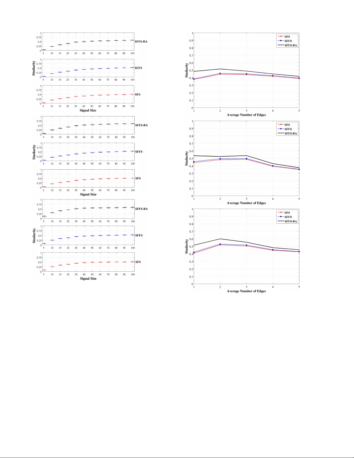
1 An iterativ e f eature selection method f or GRNs inf erence b y e xplor ing topological proper ties F abrício M. Lopes, Da vid C . Mar tins-Jr, J unior Barrera and Rober to M. Cesar-Jr F Abstract —An impor tant prob lem in bioinformatics is the inference of gene regulatory networ ks (GRN) from tempor al expression profiles . In general, the main limitations faced by GRN inference methods is the small number of samples with huge dimensionalities and the noisy nature of the expression measurements. In face of these limitations, alternatives are needed to get better accuracy on the GRNs inference problem. This work addresses this prob lem by presenting an alternative feature selection method that applies prior knowledge on its search strategy , called SFFS-BA. The proposed search strategy is based on the Sequential Floating Forward Selection (SFFS) algorithm, with the inclusion of a scale-free (Barabási-Alber t) topology information in order to guide the search process to improv e inference. The proposed algorithm e xplores the scale-free proper ty by pr uning the search space and using a power law as a weight for reducing it. In this w ay , the search space trav ersed by the SFFS-BA method combines a breadth- first search when the number of combinations is small ( h k i ≤ 2 ) with a depth-first search when the number of combinations becomes e xplosiv e ( h k i ≥ 3 ), being guided b y the scale-free pr ior inf ormation. Exper imental results show that the SFFS-BA provides a better inference similar ities than SFS and SFFS, keeping the robustness of the SFS and SFFS methods, thus presenting v er y good results . Keyw ords: SFS, SFFS, f eature selection, rev erse-engineering, gene networks inference , systems biology , bioinformatics. 1 I N T R O D U C T I O N One of the most challenging research problems for System Biology nowadays is the inference (or rev erse-engineering) of gene regulatory networks (GRNs) from expression profiles. This research issue became important after the debioinformat- icsvelopment of high-throughput technologies for extraction of gene expressions (mRNA abundances or transcripts), such as DNA microarrays [1] or SA GE [2], and more recently RN A-Seq [3]. This problem regards re vealing regulatory re- lationships between biological molecules in order to recover a complex network of interrelationships, which can describe not just div erse biological functions but also the dynamics of molecular activities. It is very important to understand how many biological processes happen and in most cases, ho w to prev ent it from happening (diseases). F .M. Lopes is with the F eder al University of T echnology - P araná, Brazil (e-mail: fabricio@utfpr .edu.br). D.C. Martins-Jr is with the F ederal University of ABC, Brazil (e- mail:david.martins@ufabc.edu.br), J. Barrera is with the F aculty of Philosophy, Sciences and Letters of Ribeirão Pr eto, University of São P aulo, Brazil (e-mail: jb@ime.usp.br). R.M. Cesar-Jr is with the Institute of Mathematics and Statistics of the University of São P aulo and Brazilian Bioethanol Science and T echnology Laboratory (CTBE), Brazil (e-mail: cesar@vision.ime.usp.br) In the context of expression profiles, a big challenge that researchers need to face is the lar ge number of v ariables or genes (thousands) for just a fe w experiments av ailable (dozens). In order to infer relationships among those variables, it is needed a great ef fort in dev eloping nov el computational and statistical techniques that are able to alleviate the intrinsic error estimation committed in the presence of small number of samples with huge dimensionalities. In general, it is not possible to recover the GRNs very accurately . The main reasons for this are the lack of informa- tion about the biological organism, the high complexity of the networks and the intrinsic noise of the expression measure- ments. In this context, there are sev eral recent initiativ es to ov ercome such limitations by incorporating other information on the inference/prediction method. One kind of initiati ve is the use of the functional gene information, e.g., from the Gene Ontology , Proteome, KEGG, among others, into the clustering process, resulting in more biologically meaningful clusters [4], [5], [6]. Another alternativ e is by using biological information for the discov ery of transcriptional regulation relationships, i.e., to infer GRNs [7], [8], [9]. A v ariety of biological data integration techniques for GRNs inference are described in [10], [11], [12], [13]. Although the integration of biological information with mathematical models is critically important in discov ering nov el biological kno wledge, it is restricted by the prior biolog- ical information of each gene or biological entity . One way to use prior information and make the methods less restrictive is the use of information about local or global prior kno wledge of an or ganism instead of an information about a single gene, e.g., to use the network structure/topology as prior information. In this way , the integrated use of multiple data types together with local and global topological properties could be decisiv e for the effecti ve prediction of GRNs and their functions in face of the known limitations [10], [14], [15], [16], [17]. The analysis of local and global biological network prop- erties and its application on the inference process is very recent and promising [18], [19], [11], [20], [21]. For example, the application of network structure by the inference methods makes use of similarities of connected network modules [22], structural and graph-theoretic interpretation for the network components [23], [17], taking into account the network sparse- ness [24], [25], [26], gene network motifs [27] and the search for cliques in network graphs [28]. More important, biological 2 networks and particularly GRNs are known not only to be sparse, but also or ganized, so as nodes belonging to different connectivity classes [29]. These examples sho w the importance of such problem and the need for ne w methodologies to ov ercome it. The information about network topology can help the inv es- tigation of biological process by adopting the complex netw ork theory and its properties [30], [31], [32], [33]. It is known that many kinds of relationships can be successfully described by complex networks. In particular , the complex networks theory describes various types of network topologies, each one with well defined properties, and it has been broadly applied to characterize biological processes and gene relationships in volv ed. Some biological networks, for example, were shown to present the scale-free property , in which many nodes have a low degree and a few of them have a high degree (hubs), in which the degree distribution is approximated by a po wer-law distribution [34], [35], [36], [37], [38], [33], [39]. In general, topological patterns and its structural analysis is one of the most promising topics in the analysis of complex networks [40], [41], and particularly the application of structural prop- erties of the network can be a very valuable prior information to be used by the GRNs inference methods. The use of network topology models for the simulation and analysis of GRNs hav e been recently described in [42] and the same models are further explored in the present paper . In this work, a new method is proposed for the inference of GRNs from expression profiles by incorporating a scale- free topology and applying a conditional dependency criterion function. Thus, it is suggested a method that takes the scale- free topology into account as prior information in the inference process. This leads to a better inference of networks presenting scale-free property . The main purpose of this paper is to show the interest of taking into account information about the scale- free topology of the network in order to improve the inference process and make it more suitable for a class of problems, i.e., scale-free networks. The inference process is conducted by observing the condi- tional dependence of a target gene gi ven its potential predictors through temporal e xpression profiles, and by applying the mean conditional entropy as criterion function [43], [44], [45], [46]. This process has been recognized as an appropriate statistical tool to model direct interactions between genes [29]. The main contribution of this work is the proposal of a new feature selection method for GRNs inference from temporal expression profiles. Our inference method is based on a previous feature selection algorithm [47], [48], with the inclusion of scale-free topology as a prior information, in which the search space trav ersed is relatively small and provides encouraging results. Next sections (Sections 2 and 3) introduce a brief back- ground on the complex network theory and the network inference problem. In Section 4, the feature selection problem is discussed in more detail, including a short description of the SFS and SFFS techniques. Section 4.3 discusses the intrinsically multiv ariate prediction issue and how it can affect the greedy feature selection algorithms in such way that the achie ved solution may be relativ ely far aw ay from the optimal. Section 6 describes our proposed feature selection method (SFFS-B A). Section 7 shows some experimental re- sults. Finally , Section 8 concludes the work, discussing future perspectiv es. 2 C O M P L E X N E T W O R K S T H E O RY A N D B I O - L O G I C A L N E T WO R K S The genes of a network can be characterized by its degree, i.e., the number of connections with other genes of these network that it has. By considering directed networks, there are two kinds distinct relationships. The in-degree is the number of directed connections recei ved by a gene. The out-degree is the number of directed connections edges sent by a gene. The indi vidual gene degrees can be used to estimate the degree distribution P ( k ) and as a result, characterize the whole network, i.e., a global network property . The uniformly-random Erdös-Rényi (ER) [49] complex network model is based on randomly connected vertices. This model assume the hypothesis that complex systems are connected at random, leading to a Poisson degree distribution with peak at the av erage degree h k i , indicating that the most of the genes have a de gree close to h k i . In other works, the ER model has a statistically homogeneous degree distribution [38]. On the other hand, the scale-free netw ork structure proposed by Barabási and Albert [50] (B A), is based on a heterogeneous distribution on its vertex degree, in which few genes hav e a large number of connections and the most of genes have few connections. The absence of a typical degree led to this complex network model to be described as “scale-free” [38]. More specifically , the scale-free structural property is charac- terized by a power -law in its connections (degree) distribution. In other words, the probability P ( k ) of a gene to interact with k other genes decays as a power law P ( k ) ∼ k − γ , (1) in which γ is a numerical constant. In general, numerous networks, such as the Internet, hu- man collaboration networks and metabolic networks, follow a scale-free structure [38]. In particular , most known biological networks present a scale-free structure [33], implying that their distribution on its gene relationships (degree k ) is irregular , a large number of connections (edges) is concentrated on a small number of genes, while large number of genes have few connections. In this case, scale-free networks hav e a high probability of exhibiting hubs [50]. In particular , by considering the transcriptional regulations of the Sacchar omyces cere visiae [35], it was found a close relation between proteins and genes which presents a degree distribution with an exponential decay very similar to a power law . In the work dev eloped by Farkas et al. [36], it was found an ov erlap between the connecti vity distribution of scale- free and Sacchar omyces cer evisiae transcriptome networks. In such work it was suggested a potential regulatory relationship among its genes, in which a small number of transcription factors are responsible for a complex set of expression patterns under div erse conditions. 3 Regarding the constant decay γ , it was reported that scale- free networks describe the Escherichia coli metabolic net- works and its metabolic reactions follo ws a power -law , with γ = 2 . 2 [34]. It is also known that the probability of a given yeast protein to interact with k other yeast proteins follows a power -law , with γ = 2 . 4 [51], [52]. In general, the degree exponent γ is usually in the range 2 < γ < 3 [31], [38]. In summary , the scale-free complex network model has been effecti v ely used to simulate and describe the behavior of biological networks [33], [34], [35], [36], [37], [38], [39]. 3 G R N I N F E R E N C E The combination of expression analysis, perturbations, treat- ments and gene mutations may indicate information about molecular or specific functions of the genes. Gene regulatory networks (GRN) inference from expression data, a process also kno wn as reverse engineering, is a dif ficult computational task due to the huge data volume (number of genes or expres- sion profiles) and to the small number of av ailable samples, including the large complexity of biological networks, thus representing an important challenge in bioinformatics and computational biology researches [53]. The GRNs inference from temporal expression data tries to identify the variation of the expression levels along time, becoming possible to indicate information such as metabolic pathways, cell cycle and mapping of modifications caused by stimuli. It can be used as a model for functional representation of gene interactions. It is important to highlight that the network inference has the objectiv e of discovering interaction networks between genes that are potentially interesting from the biological point of view . The relationships among genes are suggested according to some estimator and can be e xamined or v alidated by wet-lab experiments. As such experiments hav e a high cost in terms of financial, human and time resources, the main idea is to offer to the specialists a reduced number of hypotheses that satisfactorily identify a certain phenomenon of interest. There are se veral approaches for modeling and identification of GRNs. Examples include Boolean Networks [54] and its stochastic version (Probabilistic Boolean Networks) [55], Dif- ferential Equations [56] and Bayesian Networks [57], to name but a fe w . This work focuses on the Probabilistic Boolean Networks (PBN) model, since it captures global properties of GRNs while dealing well with settings presenting limited number of samples. Regarding the feature selection approaches to infer GRNs, there are mainly three types of criterion functions. The cor- relation based criterion functions are those that measure 1-to- 1 relationships, often employed to identify co-regulation be- tween genes, functional modules and clusters [58]. It does not take into account multiv ariate relationships, i.e., the expression of a given target being regulated by a set of two or more genes with multiv ariate interaction. Bayesian error estimation based criterion functions ev aluate the estimated errors present in the joint probability distribution of a target gene gi ven its candidate predictor genes [59], [60], [61], which is capable to detect multiv ariate (N-to-1) relationships. Finally , information theory based criterion functions are used to detect 1-to-1 and N-to-1 relationships [62], [63], [64], [45], [65], relying on the uniformity of the conditional probability distributions of the target giv en the candidate predictors as a whole (larger uniformity leads to higher entropy , which in turn leads to smaller mutual information). The literature related to modeling and identification of GRNs is huge and on rapidly increasing, which indicates its importance. The reader is referred to [11], [13], [66], [67], [68], [69] for revie ws on this subject. 4 F E AT U R E S E L E C T I O N Pattern recognition methods allow the classification of objects, i.e., a class or label is assigned to each object based on its features. In many applications, and specifically in GRN inference, the feature space dimension of such objects tends to be very high while the number of samples is very limited. In this context, the study and dev elopment of techniques for dimensionality reduction become mandatory . Feature selection is a possible approach to perform dimen- sionality reduction. A feature selection method looks for sub- sets of features that lead to a good representation, classification or prediction of the objects classes. It is composed by two main parts: a search algorithm and a criterion function which assigns a quality value to the feature subsets. The only way to guarantee optimality of the solution is to in vestigate the entire space of possible subsets (exhaustiv e search), although depending on some criterion function con- straints adopted (e.g. monotonical or U-shaped), it is possible to reach the optimal solution by searching for a constrained subset space by applying “branch-and-bound” methods [70], [71]. The e xhaustiv e search is computationally unfeasible in general, and especially for inference of GRNs which inv olves data with thousands of features (genes). There are many heuristics proposed for feature selection. T wo classical feature selection heuristics are briefly introduced and discussed below . 4.1 Sequential Forward Selection (SFS) The Sequential Forward Selection (SFS) is a genuinely greedy feature selection algorithm in the sense that it includes the best feature according to the criterion function in each step. It starts with an empty set (bottom-up approach) and adds the best indi vidual feature to the partial solution. In the next step, it looks for the best feature that, jointly with the feature already included in the partial solution, forms the best pair . This process continues until a stop condition is satisfied, which normally is based on a fixed dimension value (cardinality of the subset to be returned) or based on the variation of the criterion function from the previous to the next step. A variant of this algorithm is the Sequential Backward Selection (SBS) which starts with the full feature set and eliminates the least relev ant feature according to the criterion function (top- down approach), repeating this process successi vely until a stop condition is satisfied [47]. The greedy algorithms such as SFS and SBS present a drawback known as nesting effect. This effect occurs because the discarded features by using the top-down approach are 4 nev er inserted again to the partial solution, and the inserted features in the bottom-up approach are never discarded from the partial solution. Section 4.3 presents the reason why this phenomenon occurs. 4.2 Sequential Floating Forward Selection (SFFS) The Sequential Floating Forward Selection (SFFS) algorithm tries to alleviate the nesting effect by allowing the inclusion and exclusion of features in the partial solution in a floating way , i.e., without requiring the definition of the number of insertions or exclusions [47]. It starts with an empty set (cardinality k = 0). The SFS algorithm is applied until k = 2. For k > 2, the SBS algorithm is applied in order to exclude bad features. The SFFS applies alternately the SFS and SBS until a stop condition is reached. The best solution of each cardinality k is stored in a list. The best solution among them is selected as the returned solution of the algorithm and, in case of ties, the solution with the smallest cardinality is returned. A schematic flowchart of the SFFS algorithm is presented in Figure 1. Fig. 1. Schematic flowchar t of the SFFS algor ithm [46] (adapted from [72]). K ref ers to the size of the current solution subset while d refers to the size of the final solution subset. SFFS is renowned for presenting an excellent cost-benefit in terms of the computational complexity and the quality of the returned solution. There are some variants of this algorithm (adaptiv e and generalized floating search methods) that try to improve the SFFS solutions at the expense of an increase on the computational cost. Howe ver , they can not avoid the nesting effect completely [72]. 4.3 Intrinsically Multivariate Prediction This section briefly discusses one of the main reasons why the feature selection heuristics do not guarantee the optimum solution. A target feature is intrinsically multiv ariate predicted (IMP) by its predictor feature set if all predictors combined greatly predicts the target behavior , while every properly contained subset of the mentioned predictor set has an almost null prediction power regarding the target. Formally , a set of features X is intrinsically multiv ariate predictiv e for the target feature Y with respect to λ and δ , for 0 ≤ λ , δ ≤ 1 and λ < δ , if max Z & X F Y ( Z ) ≤ λ ∧ F Y ( X ) ≥ δ (2) where F is a criterion function that varies from 0 to 1 (0 meaning absence of prediction and 1 meaning full prediction) [73]. The parameters λ and δ usually assume small (less than 0.2) and large (greater than 0.8) values, respectiv ely , to reflect the IMP property . Additionally , an intrinsically multiv ariate predictiv eness degree (IMP score) through the maximum value of δ − λ can be defined as: I Y ( X ) = F Y ( X ) − max Z & X F Y ( Z ) (3) Considering Boolean features, the deterministic e xclusiv e-or binary logic (XOR) is an e xample of an IMP set when tw o pre- dictors may assume an y value from { ( 0 , 0 ) , ( 0 , 1 ) , ( 1 , 0 ) , ( 1 , 1 ) } with uniform probability distribution. In this case, it is impos- sible to predict the target based on the observation of just one of its predictors, since the target can assume the value 0 or 1 regardless of the v alues of each individual predictor . Of course when the predictors are combined, the prediction is perfect for ev ery instance from { ( 0 , 0 ) , ( 0 , 1 ) , ( 1 , 0 ) , ( 1 , 1 ) } (the prediction is giv en by the XOR logic). The nesting ef fect occurs in most feature selection algo- rithms and can be explained by the IMP phenomenon. Consid- ering an IMP set, its individual features (or subsets of features) are not good to predict the target, so they hardly will be included in the partial solution of a giv en sub-optimal feature selection. Howe v er , an optimum solution can be formed by such features together (large IMP score), which implies that the considered feature selection probably does not reach this solution. Besides, two good indi vidual predictors may not lead to a very good pair, since they have a relativ ely high correlation with the target feature, meaning that they hav e high correlation with each other . Section 6 shows that the method proposed here can ev entually return IMP sets as solutions when its IMP score is moderately large, i.e., each individual feature has little, but not null, contribution in predicting the target feature, and also when the cardinality of such IMP sets is not very high (in this case, any good predictor set with large cardinality would not be returned due to the high estimation error performed when ev aluating large dimensionality sets). 5 P R O B A B I L I S T I C G E N E T I C N E T W O R K S Probabilistic Genetic Networks (PGN) is a model proposed to represent GRNs. PGNs are based on PBNs, in which the selection of the transition function is not deterministic and the states of the genes and networks are represented by discrete values. PGNs describe a finite dynamical system, discrete in time, composed by a finite number of states, in which each transcript is represented by a variable. The composition of all v ariables form a vector considered the system state. Each vector component has an associated transition function which calculates its next value from the previous state of other genes (predictors). These functions are components of a transition functions vector , which defines the transition from a network state to the next state and represents the gene regulation mechanism [45]. In this model, the gene expression networks are represented as a stochastic process ruled by a Markov chain. In other 5 words, assuming this principle means that a conditional prob- ability of a future event, given the previous events, depends only on the immediately previous ev ent. A Markov chain is characterized by a transition matrix π Y | X of conditional probabilities among states, and its elements are denoted by p y | x , and a vector of initial states s 0 . A PGN is a Markov chain ( π Y | X , s 0 ) in which some axioms are assumed [45]: i the transition matrix π Y | X is homogeneous, i.e., p y | x is not a function of t . The state transition probability is constant; ii p y | x > 0, i.e., all state pairs can be reached (er godic Markov chain); iii the transition matrix π Y | X is conditionally independent, i.e., for ev ery state pair x , y , p y | x = ∏ n i = 1 p ( y i | x ) ; iv π Y | X is quasi-deterministic, i.e., for e very state x , exists a state y such that p y | x ≈ 1. Theses axioms are moti vated by biological phenomena or simplifications due to the lack of samples for model estima- tion. The first axiom is a constraint to simplify the estimation problem. The second axiom states that all states are reachable, i.e., the presence of perturbation or noise can ev entually lead the system to any state. The third axiom determines that a gene expression at a gi ven time instant is independent of the expression of other genes at the same instant t . The last axiom says that the system has a structural dynamics which is prone to small noises [45]. 6 S F F S W I T H S T R U C T U R A L P R O P E R T I E S ( S F F S - B A ) The proposed method is based on the Probabilistic Genetic Networks (PGN), which is described in [45] and in Section 5. The proposed method considers the four axioms established by the PGN model and proposes two new constraints: • For every target gene i , by adding a new predictor x i in the result set with cardinality > 1, there should be an information gain in the prediction of the target gene, whenev er the chosen predictor is part of the true result set. If the information gain by adding a new predictor in the result set is poor , the predictor could not be part of the true result set or there is no data enough to make the prediction. In both cases, the inclusion of the predictor in the result set should be a voided. • The network topology follows a power-la w in its connec- tions distribution, i.e., a scale-free network structure such as described in Section 2. By assuming the PGN model and these new constraints, the main contribution of our method is to include structural information as a prior knowledge to perform a search on a reduced space, thus achieving better results. The idea is based on the assumption that a gene with no predictors tends to have a random behavior , while a gene with predictors tends to hav e a more ordered behavior . In this way , it is possible to expect that a source gene in a GRN (i.e., with no predictors) presents a behavior with small variations in the criterion function on trying to identify a possible predictor to it. In other w ords, small v ariations are expected on the criterion function values by adding ne w predictors on the result set of a source, as shown by Figure 2 (Source). Fig. 2. Criter ion function behavior by the inclusion of new predictors in the result set (optimum value is zero). The blac k curve (Normal) is expected f or targets with well defined predictors in which each predictor has a good contribution in predicting the target behavior . The blue cur v e (IMP) is e xpected f or targets with intrinsically multiv ariate predictors in which each predictor is not good enough to predict the target behavior , as opposite to the whole predictor set. The red cur v e (Source) is expected f or targets that hav e no predictors. On the other hand, when a gene has predictors, it is expected a distinct beha vior , mainly on trying a possible predictor that is part of the result set (true positiv e). In this way , it is expected some significant variation on criterion function values when performing a search for possible predictors, as showed by Figure 2 (Normal and IMP). The curves shown in Figure 2 were obtained using the A GN model described in [42], for which it was applied the mean conditional entropy as a criterion function [46] in order to exemplify the adopted assumption for the three discussed cases, i.e., normal, source and IMP . Giv en the network topology constraint and the IMP prop- erty , the proposed algorithm performs a search for best and worst individual predictors, based on the SFFS-MR algorithm [48], by considering all genes of the network. SFFS-MR is an algorithm that applies the classical SFFS for several initial features, considering good and bad individual features. In the second step, the search is performed again for all genes, b ut the algorithm chooses the target genes that present a prediction gain (i.e., the criterion function v alue moves closer to the optimum) by adding a new predictor to its result set. This increased result set is preserv ed in the ne xt iteration. The tar get genes with small information gain, i.e., poor predictions when increasing its predictor set, are not considered for the next iteration, as well as the predictor set that reaches the optimal value of the criterion function or gets too close to it. In this context, the scale-free topology and the above pre- sented assumption are considered by the proposed algorithm in order to integrate the prior knowledge (scale-free topology), applied to reverse-engineering of GRNs from temporal expres- sion profiles. By considering that the scale-free network model 6 is characterized by a power law P ( k ) ≈ k − γ in its connections distribution (Section 2), the same power law is considered to prune the search space on each iteration. Algorithm 1 Network-Inference ( t arge t s , e x ps , γ , ∆ ) 1: var list exel is t 2: var inte ger k ← 1, n ← t arge t s .size() 3: f or i = 1 to n do 4: exel is t .append( t arge t s [ i ] , / 0, 1, 0) 5: end for 6: while n > 1 do 7: for i = 1 to n do 8: [ t ar ge t , pset s , c f v , gain ] ← e xel ist .removefirst() 9: [ new pset s , newc f v , gain ] ← SFFS- B A( t arg et , c f v , pse t s , k , e x ps , ∆ ) 10: ex elist.append( t arge t , new pset s , newc f v , gain ) 11: end for 12: SortPredictorSetsbyGain(ex elist) 13: n ← n × k − γ 14: k ← k + 1 15: end while 16: r eturn e xel ist Algorithm 2 SFFS-B A ( t arge t , c f v , pse t s , k , e x ps , ∆ ) 1: if pse t s = / 0 then 2: for pred ict or id x = 1 to ex ps .size() do 3: pset s .append( pred ict or id x ) 4: end for 5: end if 6: while pse t s is not empty and pset s .first.cardinality ≤ k do 7: new pset ← pset s .remov efirst() 8: newc f v ← SFS( t ar ge t , new pse t , k , e x ps ) 9: if newc f v < bes t c f v and ( best c f v − newc f v ) > ∆ then 10: newc f v ← SBS( t ar ge t , new pse t , ex ps ) 11: best c f v ← newc f v 12: best se t ← new pset 13: end if 14: if new pset .cardinality = 1 then 15: pset s .append( new pset ) 16: end if 17: end while 18: if k > 1 then 19: pset s ← best set 20: end if 21: r eturn [ pset s , best c f v , ( c f v − best c f v ) ] Algorithm 1 starts by considering the targets and all av ail- able samples (temporal e xpression profile, called exps ) in order to select the individual predictors, i.e., k = 1. In the following, Algorithm 2 (SFFS-BA) is applied in order to discover the best features of each target gene, which are ranked according to the adopted criterion function. One important difference of the proposed feature selection method is that the algorithm will explore the search space in steps, i.e., the predictors are chosen iteratively according to the cardinality parameter k . Another dif ference is that for k = 1 the SFFS-B A algorithm will return all predictor sets and the best criterion function value in order to explore all the individual predictors in the next iteration and to better recover the predictors of the IMP targets. From k > 1, the algorithm begins to return only the best set, assuming that some of the true predictors would be in the selected predictors set. At the end of each iteration of the Algorithm 1, the target genes are sorted by the prediction gain, the number of considered targets for the next iteration is updated following a po wer law , gi ven by n = n × k − γ and the cardinality of the result set is updated ( k ← k + 1). In this way , when k = 2, the next iterations will consider just the target genes with higher prediction gain when increasing its predictor cardinality k . It is important to notice that target genes that reach the optimal v alue of criterion function or get too close are not considered for the increasing on its predictor cardinality . The search is performed while the number of tar get genes n > 1 (stop condition). In summary , the SFFS-BA differs from SFFS (Section 4.2) because of its iterati vity , the exploration of all combinations of predictors set with cardinality k ≤ 2 and the inclusion of a search space pruning method based on the assumption that the expression data (input) were generated from a scale-free network. Algorithms 1 and 2 present the specification of the proposed feature selection algorithm: SFFS-BA. The parameter ex ps represents the temporal expression profile, in which the genes are generally arranged in the rows and experiments in the columns. The parameter γ is a constant value that determines the exponential decay , i.e., the number of targets that will be considered in the next iteration (predictor set expansion). A criterion function value variation ( ∆ ) is also included. The ∆ value prev ents that minor variations of the criterion function ( ≤ ∆ ) cause the increase of the predictors subset. The present paper adopted γ = 2 . 5 and ∆ = 0 . 05. The adopted γ is related with the mean v alue found in the literature, which is usually in the range 2 < γ < 3 [31], [38]. The application of the algorithm to predict a single gene or a set of genes of interest instead of the entire network is straightforward by selecting the targets parameter . 7 E X P E R I M E N TA L R E S U L T S This section presents the experimental results obtained by con- sidering a synthetic networks approach, which is described in [42]. The artificial gene networks (A GNs) were generated by considering the uniformly-random Erdös-Rényi (ER) topology , the scale-free Barabási-Albert (B A) and the small-world W atts- Strogatz (WS). For all experiments, the network models (ER, BA and WS) were applied with n = 100 vertices (genes). The a verage degree h k i per gene varied from 1 to 5, and the number of observed time instants (signal size) varied from 5, 10, 15, 20 to 100 in steps of 20. For each gene g i of the network, its value was giv en by a randomly selected function from 3 possible Boolean functions { f ( i ) 1 , f ( i ) 2 , f ( i ) 3 } , which represents different behaviors or functions assumed by each gene g i . In order to 7 assign a robust structural dynamics with small noise to the networks, the probabilities of each function be selected are giv en by c ( i ) 1 = 0 . 98 , c ( i ) 2 = 0 . 01 , c ( i ) 3 = 0 . 01 , i = 1 , . . . , n . W ith these probabilities, the PGN axioms ii (all possible states are reachable) and iv (quasi-deterministic setting) are satisfied (Section 5). The network identification method described in [46] im- plements feature selection methods for network inference. By applying the SFS and SFFS as search strategies and the mean conditional entropy as criterion function. This method was applied in order to identify the networks from simulated temporal expressions. The same method, criterion function and other parameters (default) were kept fixed during the comparativ e analysis with SFFS-BA. In order to measure the similarity between the synthetic ( A ) and the inferred ( B ) networks, we adopt the PP V (Pos- itiv e Predictiv e V alue, also kno wn as accuracy or precision) and Sensit ivit y (or recall) [74], [42], which are widely used to compare the results of the GRNs inference methods. Since the PP V and Sensit ivit y are not independent of each other , we take into account the geometrical mean between them as a similarity measure, given by: Simil ar i t y ( A , B ) = p PP V ( A , B ) × S ensi t ivit y ( A , B ) . The experimental results were obtained from 50 simulations by using different signal sizes (i.e., number of time points) and h k i v alues. The first experiment was performed in order to compare the three methods (SFS, SFFS and SFFS-BA) with respect to the temporal expressions size, which is a critical issue in bioinformatics problems. Figure 3 presents these results, in which the similarity measure was calculated by taking into account the average results for all variations of h k i . It is possible to notice that all methods hav e an increase on its performance by increasing the number of observ ations in the three network topologies (ER, WS and B A). Howe ver , the improv ement of the SFFS-BA occurs earlier by using just 20 time points, consistently outperforming the other two meth- ods from this point forward. Meanwhile, the SFFS slightly outperforms the SFS only with the signal size greater than 80 time points, i.e., the difference of the similarity rates is smaller than the difference achiev ed by SFFS-B A by considering all network topologies. In addition, the SFFS-B A similarity curve (Figure 3) shows a more significant improvement with the expansion on signal size by considering the BA network topology , as expected. Howe v er , considering ER and WS network topologies, the improv ement of the SFFS-BA not only outperforms the other two methods but also it is consistent, ev en in the presence of some perturbations in the temporal signal, which is implied by the stochasticity in the application of transition functions. Figure 4 (a) and (b) shows the boxplots of the similarity values for each number of time points. It is possible to notice a very small variation in the boxplots, indicating stable results for all time points. These results are an important indicati ve of the stability of the proposed methodology . The second experiment was performed in order to compare the robustness of the methods by increasing the complexity of the networks in terms of its av erage degree h k i . Figure (a) ER (b) WS (c) B A Fig. 3. Similarity measure obtained by SFS, SFFS and SFFS-BA applied to infer networ k edges from temporal e xpression profiles with different number of time points (signal size). The similar ity represents the mean over 50 e xecutions f or each netw ork topology . 5 presents the a verage results for all variations of signal size (number of time points). It is possible to notice the similarity down-grade with the increase of av erage degree h k i for the three algorithms. Howe ver , there was an improvement in results from h k i = 1 to h k i = 2 for ER and B A topologies. This behavior can be explained by the fact that less complex networks h k i = 1 have several genes with no predictor , but the inference methods tend to find false positiv es, thus reducing its similarity ratio. In this context, the SFFS-BA algorithm also outperforms the SFS and SFFS, presenting a soft decrease of similarity with the increase of av erage degree h k i for ER topology . In 8 (a) ER (b) WS (c) B A Fig. 4. Distr ib ution (boxplots) of the similar ity values obtained by SFS, SFFS and SFFS-BA applied to infer network edges from temporal expression profiles with diff erent number of time points (signal size) from 50 e xecutions of each netw ork topology . the presence of a network structure as is the case of BA and WS topologies, the decrease of similarity was less smooth, but ev en in these cases the SFFS-BA presents better results. W ith regard to the IMP genes with cardinality greater or equal than 3, it is important to notice that the SFFS-BA tends to consider them if, at each step, an individual predictor added to the subset has a prediction gain larger than the predictors of the genes considered as sources (absence of predictors). The tendency is that a moderately IMP set is detected if the number of samples contained in the gene expression matrix is suf ficient to estimate its joint probability distributions. Howe ver , there are two situations in which it is possible that SFFS-BA considers the target gene from an IMP set as source gene. The first situation is the case in which the dimension of the IMP (a) ER (b) WS (c) B A Fig. 5. Similarity measure obtained by SFS, SFFS and SFFS-BA applied to inf er network edges from different network comple xities in terms of av erage degree h k i . The similarity represents the mean over 50 ex ecutions for each network topology . set is excessiv e for the number of samples av ailable, making the error estimation of the joint probability distributions a crucial factor (the number of parameter to be estimated grows exponentially as a function of the cardinality). The second case refers to the strongly IMP sets where all its properly contained subsets offer a very poor information gain with regard to the target. This problem is inherent to the feature selection methods that explore only a subspace of all possible solutions, as SFFS-BA does. The only way to guarantee that IMP features are returned is through a exhausti ve search for the whole solution space. 9 8 C O N C L U S I O N This work presents an iterativ e floating search strategy for the inference of gene regulatory networks by including the scale- free assumption as a prior information in the inference process. Giv en the kno wn limitations, our focus is the inclusion of prior knowledge on search methods. In particular, by presenting a more suitable and efficient algorithm for the inference of GRNs from temporal expression profiles, which presents a small number of samples and huge dimensionalities (genes). The proposed algorithm is based on the assumption that sev eral biological networks can be approximated by a scale- free topology . The presented method exploits this property by pruning the search space and using a power law as a weight for reducing the search space. In this context, the search space trav ersed by the SFFS-B A method combines a breadth-first search when the number of combinations is small ( h k i ≤ 2) with a depth-first search when the number of combinations becomes explosi ve ( h k i ≥ 3). The experimental results sho w that the SFFS-BA provides better inference accuracy than SFS and SFFS, when consid- ering small signal sizes with 20-30 time points and also with large ones, with 100 time points. In addition, the SFFS-B A was able to achieve 60% of similarity on network recovery after only 50 observations from a state space of size 2 20 , presenting very good results. The SFFS-BA has also prov ed to be robust and stable, as SFS and SFFS, when submitted to the increasing complexity of the networks in terms of its average degree h k i . The robust- ness ans stability are important properties for the inference methods, even in the presence of some perturbations in the temporal signal, implied by the stochasticity in the application of transition functions. Besides, the SFFS-B A showed better results than the SFS and SFFS. A possible extension of the present work would be the inclusion of the small-world (WS) [75] topology information in order to guide the search process for the correct topology inference of these networks. Also, we plan to apply this technique to infer GRNs from real data. A C K N OW L E D G M E N T S This work was supported by F APESP , CNPq and CAPES. R E F E R E N C E S [1] D. Shalon, S. J. Smith, and P . O. Brown, “A DNA microarray system for analyzing complex DNA samples using two-color fluorescent probe hybridization.” Genome Researc h , vol. 6, no. 7, pp. 639–645, 1996. [2] V . E. V elculescu, L. Zhang, B. V ogelstein, and K. W . Kinzler, “Serial Analysis of Gene Expression, ” Science , vol. 270, no. 5235, pp. 484–487, 1995. [3] Z. W ang, M. Gerstein, and M. Snyder , “RNA-Seq: a revolutionary tool for transcriptomics, ” Nat Rev Genet , vol. 10, no. 1, pp. 57–63, 2009. [4] G. Macintyre, J. Bailey , D. Gustafsson, I. Havi v , and A. K ow alczyk, “Using gene ontology annotations in exploratory microarray clustering to understand cancer etiology , ” P attern Recognition Letters , vol. In Press, Corrected Proof, pp. –, 2010. [5] X. Cui, T . W ang, H.-S. Chen, V . Busov , and H. W ei, “Tf-finder: A software package for identifying transcription factors inv olved in biological processes using microarray data and existing knowledge base, ” BMC Bioinformatics , vol. 11, no. 1, p. 425, 2010. [6] J. De Haan, E. Piek, R. van Schaik, J. de Vlieg, S. Bauerschmidt, L. Buydens, and R. W ehrens, “Integrating gene expression and go classification for pca by preclustering, ” BMC Bioinformatics , vol. 11, no. 1, p. 158, 2010. [7] A. V . W erhli and D. Husmeier, “Gene regulatory network reconstruction by bayesian integration of prior knowledge and/or different experimental conditions, ” Journal of Bioinformatics and Computational Biology , vol. 6, no. 3, pp. 543–572, 2008. [8] J. Ernst, Q. K. Beg, K. A. Kay , G. Balázsi, Z. N. Oltvai, and Z. Bar- Joseph, “ A semi-supervised method for predicting transcription factor- gene interactions in Escherichia coli , ” PLoS Comput Biol , vol. 4, no. 3, p. e1000044, 03 2008. [9] J. Seok, A. Kaushal, R. Davis, and W . Xiao, “Knowledge-based analysis of microarrays for the discovery of transcriptional regulation relation- ships, ” BMC Bioinformatics , vol. 11, no. Suppl 1, p. S8, 2010. [10] O. G. T royanskaya, “Putting microarrays in a context: Inte grated analysis of diverse biological data, ” Brief Bioinform , vol. 6, no. 1, pp. 34–43, 2005. [11] G. Karlebach and R. Shamir, “Modelling and analysis of gene regulatory networks, ” Nat Rev Mol Cell Biol , vol. 9, no. 10, pp. 770–780, 2008. [12] J. Baumbach, A. T auch, and S. Rahmann, “T o wards the integrated analysis, visualization and reconstruction of microbial gene regulatory networks, ” Brief Bioinform , vol. 10, no. 1, pp. 75–83, 2009. [13] M. Hecker, S. Lambeck, S. T oepfer , E. van Someren, and R. Guthke, “Gene regulatory network inference: Data integration in dynamic models - A revie w, ” Biosystems , vol. 96, no. 1, pp. 86–103, 2009. [14] M. V idal, “Interactome modeling, ” FEBS Letters , vol. 579, no. 8, pp. 1834–1838, 2005, systems Biology . [15] T . Aittokallio and B. Schwikowski, “Graph-based methods for analysing networks in cell biology, ” Brief Bioinform , vol. 7, no. 3, pp. 243–255, 2006. [16] S. Ray , S. Bandyopadhyay , and S. Pal, “Combining multisource infor- mation through functional-annotation-based weighting: Gene function prediction in yeast, ” Biomedical Engineering, IEEE T ransactions on , vol. 56, no. 2, pp. 229–236, 2 2009. [17] O. Kuchaie v , T . Milenkovic, V . Memisevic, W . Hayes, and N. Przulj, “T opological network alignment uncovers biological function and phy- logeny , ” Journal of The Royal Society Interface , vol. 7, no. 50, pp. 1341–1354, March 2010. [18] S. Klamt, J. Saez-Rodriguez, and E. Gilles, “Structural and functional analysis of cellular networks with cellnetanalyzer, ” BMC Systems Biol- ogy , vol. 1, no. 1, p. 2, 2007. [19] V . Lacroix, L. Cottret, P . Thébault, and M.-F . Sagot, “ An introduction to metabolic networks and their structural analysis, ” IEEE/A CM T rans. Comput. Biol. Bioinformatics , vol. 5, no. 4, pp. 594–617, 2008. [20] P . Lenas, M. Moos, and F . P . Luyten, “Developmental engineering: A new paradigm for the design and manufacturing of cell-based products. part ii. from genes to networks: Tissue engineering from the viewpoint of systems biology and network science, ” T issue Engineering P art B: Reviews , vol. 15, no. 4, pp. 395–422, 2009. [21] T . Przytycka and Y .-A. Kim, “Network integration meets network dynamics, ” BMC Biology , vol. 8, no. 1, p. 48, 2010. [22] I. Ulitsky and R. Shamir, “Identification of functional modules using network topology and high-throughput data, ” BMC Systems Biology , vol. 1, no. 1, p. 8, 2007. [23] S. Narasimhan, R. Rengaswamy , and R. V adigepalli, “Structural prop- erties of gene regulatory networks: Definitions and connections, ” IEEE/ACM T rans. Comput. Biol. Bioinformatics , vol. 6, no. 1, pp. 158– 170, Jan.-March 2009. [24] M. Andrecut and S. Kauffman, “On the sparse reconstruction of gene networks, ” Journal of Computational Biology , vol. 15, no. 1, pp. 21–30, 2008. [25] M. Andrecut, S. Huang, and S. Kauffman, “Heuristic approach to sparse approximation of gene regulatory networks, ” Journal of Computational Biology , vol. 15, no. 9, pp. 1173–1186, 2008. [26] S. Christley , Q. Nie, and X. Xie, “Incorporating existing network information into gene network inference, ” PLoS ONE , vol. 4, no. 8, p. e6799, 08 2009. [27] S. Ott, A. Hansen, S.-Y . Kim, and S. Miyano, “Superiority of network motifs over optimal networks and an application to the revelation of gene network evolution, ” Bioinformatics , vol. 21, no. 2, pp. 227–238, 2005. [28] H. Y u, A. Paccanaro, V . Trifono v , and M. Gerstein, “Predicting inter- actions in protein networks by completing defective cliques, ” Bioinfor- matics , vol. 22, no. 7, pp. 823–829, 2006. 10 [29] C. Charbonnier , J. Chiquet, and C. Ambroise, “W eighted-lasso for struc- tured network inference from time course data, ” Statistical Applications in Genetics and Molecular Biology , vol. 9, no. 1, p. 15, 2010. [30] S. H. Strogatz, “Exploring complex networks, ” Nature , vol. 410, no. 6825, pp. 268–276, 2001. [31] R. Albert and A.-L. Barabási, “Statistical mechanics of complex net- works, ” Rev . Mod. Phys. , vol. 74, no. 1, pp. 47–97, 2002. [32] M. E. J. Newman, “The structure and function of complex networks, ” SIAM Review , vol. 45, no. 2, pp. 167–256, 2003. [33] L. d. F . Costa, F . A. Rodrigues, and A. S. Cristino, “Complex networks: the key to systems biology , ” Genetics and Molecular Biology , vol. 31, no. 3, pp. 591–601, 2008. [34] H. Jeong, B. T ombor, R. Albert, Z. N. Oltvai, and A.-L. Barabási, “The large-scale organization of metabolic networks, ” Nature , vol. 407, pp. 651–654, 2000. [35] N. Guelzim, S. Bottani, P . Bourgine, and F . Képès, “T opological and causal structure of the yeast transcriptional regulatory network, ” Nature genetics , vol. 31, pp. 60–63, 2002. [36] I. J. Farkas, H. Jeong, T . V icsek, A.-L. Barabási, , and Z. N. Oltvai, “The topology of the transcription regulatory network in the yeast, saccharomyces cerevisiae, ” Physica A: Statistical Mechanics and its Applications , vol. 318, no. 3-4, pp. 601–612, 2003. [37] A.-L. Barabási and Z. Oltvai, “Network biology: Understanding the cell’ s functional or ganization, ” Natur e Re views Genetics , v ol. 5, pp. 101– 113, February 2004. [38] R. Albert, “Scale-free networks in cell biology, ” J Cell Sci , vol. 118, no. 21, pp. 4947–4957, 2005. [39] A.-L. Barabási, “Scale-Free Networks: A Decade and Beyond, ” Science , vol. 325, no. 5939, pp. 412–413, 2009. [40] U. Alon, “Network motifs: theory and experimental approaches, ” Nat Rev Genet , vol. 8, no. 6, pp. 450–461, 2007. [41] B. Goemann, E. Wingender , and A. Potapov , “ An approach to ev aluate the topological significance of motifs and other patterns in regulatory networks, ” BMC Systems Biology , vol. 3, no. 1, p. 53, 2009. [42] F . M. Lopes, R. M. Cesar-Jr , and L. d. F . Costa, “Gene expression complex networks: synthesis, identification and analysis, ” Journal of Computational Biology , vol. In Press, Accepted Manuscript, 2011. [43] S. Liang, S. Fuhrman, and R. Somogyi, “Reveal: a general reverse engineering algorithm for inference of genetic network architectures, ” in Pr oceedings of the P acific Symposium on Biocomputing , 1998, pp. 18– 29. [Online]. A vailable: http://psb.stanford.edu/psb- online/proceedings/ psb98/abstracts/p18.html [44] D. C. Martins-Jr, R. M. Cesar-Jr , and J. Barrera, “W -operator window design by minimization of mean conditional entropy , ” P attern Analysis & Applications , vol. 9, pp. 139–153, 2006. [45] J. Barrera, R. M. Cesar-Jr , D. C. Martins-Jr, R. Z. N. V encio, E. F . Merino, M. M. Y amamoto, F . G. Leonardi, C. A. B. Pereira, and H. A. Portillo, “Constructing probabilistic genetic networks of Plasmodium falciparum , from dynamical expression signals of the intraerythrocytic dev elopment cycle, ” in Methods of Microarr ay Data Analysis V , P . Mc- Connell, S. M. Lin, and P . Hurban, Eds. Springer US, 2007, pp. 11–26. [46] F . M. Lopes, D. C. Martins-Jr , and R. M. Cesar-Jr , “Feature selection en vironment for genomic applications, ” BMC Bioinformatics , v ol. 9, no. 1, p. 451, October 2008. [47] P . Pudil, J. Novo vi ˇ cová, and J. Kittler, “Floating search methods in feature-selection, ” P attern Recognition Letters , v ol. 15, no. 11, pp. 1119– 1125, November 1994. [48] F . M. Lopes, D. C. Martins-Jr, J. Barrera, and R. M. Cesar-Jr , “SFFS- MR: a floating search strategy for GRNs inference, ” in P attern Recogni- tion in Bioinformatics, Proceedings , ser . Lecture Notes in Computer Sci- ence, vol. 6282. Springer Berlin / Heidelberg, 2010, Proceedings Paper , pp. 407–418, 5th IAPR International Conference on Pattern Recognition in Bioinformatics (PRIB 2010), Nijmegen, The Netherlands, SEP 22-24, 2010. [49] P . Erdös and A. Rényi, “On random graphs, ” Publ. Math. Debrecen , vol. 6, pp. 290–297, 1959. [50] A.-L. Barabási and R. Albert, “Emergence of scaling in random net- works, ” Science , vol. 286, no. 5439, pp. 509–512, 1999. [51] H. Jeong, S. P . Mason, A.-L. Barabási, and Z. N. Oltvai, “Lethality and centrality in protein networks, ” Natur e , vol. 411, no. 6833, pp. 41–42, 2001. [52] S. Boccaletti, V . Latora, Y . Moreno, M. Chavez, and D. U. Hwang, “Complex netw orks: Structure and dynamics, ” Physics Reports , vol. 424, no. 4-5, pp. 175–308, 2006. [53] I. Hov atta, K. Kimppa, A. Lehmussola, T . Pasanen, J. Saarela, I. Saarikko, J. Saharinen, P . T iikkainen, T . T oi vanen, M. T olvanen et al. , DNA micr oarray data analysis , 2nd ed. CSC, Scientific Computing Ltd, 2005. [54] S. A. Kauffman, “Metabolic stability and epigenesis in randomly con- structed genetic nets, ” Journal of Theoretical Biology , vol. 22, no. 3, pp. 437–467, March 1969. [55] I. Shmule vich, E. R. Dougherty , S. Kim, and W . Zhang, “Probabilistic boolean networks: a rule-based uncertainty model for gene regulatory networks, ” Bioinformatics , vol. 18, no. 2, pp. 261–274, 2002. [56] T . Chen, H. L. He, and G. M. Church, “Modeling gene expression with differential equations, ” in P acific Symposium on Biocomputing , 1999, pp. 29–40. [57] N. Friedman, M. Linial, I. Nachman, and D. Pe’er, “Using bayesian networks to analyze e xpression data, ” Journal of Computational Biology , vol. 7, no. 3-4, pp. 601–620, 2000. [58] J. M. Stuart, E. Segal, D. K oller , and S. K. Kim, “ A gene-coexpression network for global discovery of conserved genetic modules, ” Science , vol. 302, no. 5643, pp. 249–255, 2003. [59] R. F . Hashimoto, S. Kim, I. Shmulevich, W . Zhang, M. L. Bittner, and E. R. Dougherty , “Growing genetic regulatory networks from seed genes, ” Bioinformatics , vol. 20, no. 8, pp. 1241–1247, May 2004. [60] E. R. Dougherty , M. Brun, J. M. T rent, and M. L. Bittner , “Conditioning- based modeling of contextual genomic regulation, ” IEEE/ACM TCBB , vol. 6, pp. 310–320, 2009. [61] N. Ghaffari, I. Ivanov , X. Qian, and E. R. Dougherty , “A CoD-based reduction algorithm for designing stationary control policies on Boolean networks, ” Bioinformatics , vol. 26, no. 12, pp. 1556–1563, Apr 2010. [62] A. Margolin, K. N. Basso, C. Wiggins, G. Stolovitzky , R. Favera, and A. Califano, “ARACNE: An algorithm for the reconstruction of gene regulatory networks in a mammalian cellular context, ” BMC Bioinformatics , vol. 7, no. Suppl 1, p. S7, 2006. [63] J. Faith, B. Hayete, J. Thaden, I. Mogno, J. W ierzbowski, G. Cottarel, S. Kasif, J. Collins, and T . Gardner, “Lar ge-scale mapping and validation of escherichia coli transcriptional regulation from a compendium of expression profiles, ” PLoS Biology , vol. 5, no. 1, pp. 259–265, 2007. [64] A. Rao, A. Hero III, D. States, and J. Engel, “Using directed information to build biologically relev ant influence networks, ” in Pr oc LSS Comput Syst Bioinform , August 2007, pp. 145–156. [Online]. A v ailable: http://www .lifesciencessociety .org/CSB2007/toc/PDF/145.2007.pdf [65] W . Zhao, E. Serpedin, and E. R. Dougherty , “Inferring connecti vity of genetic regulatory networks using information-theoretic criteria, ” IEEE/ACM TCBB , vol. 5, no. 2, pp. 262–274, April 2008. [66] P . D’haeseleer , S. Liang, and R. Somogyi, “Genetic network inference: from co-expression clustering to reverse engineering, ” Bioinformatics , vol. 16, no. 8, pp. 707–726, 2000. [67] H. de Jong, “Modeling and simulation of genetic regulatory systems: A literature revie w , ” Journal of Computational Biology , vol. 9, no. 1, pp. 67–103, 2002. [68] M. P . Styczynski and G. Stephanopoulos, “Overvie w of computational methods for the inference of gene regulatory networks, ” Computers & Chemical Engineering , vol. 29, no. 3, pp. 519–534, 2005. [69] T . Schllit and A. Brazma, “Current approaches to gene regulatory network modelling, ” BMC Bioinformatics , vol. 8, no. Suppl 6, p. S9, September 2007. [70] P . Somol, P . Pudil, and J. Kittler , “Fast branch & bound algorithms for optimal feature selection, ” IEEE TP AMI , vol. 26, no. 7, pp. 900–912, July 2004. [71] M. Ris, D. C. Martins-Jr, and J. Barrera, “U-curve: A branch-and-bound optimization algorithm for u-shaped cost functions on boolean lattices applied to the feature selection problem, ” P attern Recognition , vol. 43, no. 3, pp. 557–568, March 2010. [72] P . Somol, P . Pudil, J. Novo vi ˇ cová, and P . Paclík, “ Adapti ve float- ing search methods in feature selection, ” P attern Recognition Letters , vol. 20, pp. 1157–1163, 1999. [73] D. C. Martins-Jr, U. Braga-Neto, R. F . Hashimoto, E. R. Dougherty , and M. L. Bittner, “Intrinsically multi variate predicti ve genes, ” IEEE J ournal of Selected T opics in Signal Pr ocessing , vol. 2, no. 3, pp. 424–439, June 2008. [74] E. R. Dougherty , “V alidation of inference procedures for gene regulatory networks, ” Current Genomics , vol. 8, no. 6, pp. 351–359, 2007. [75] D. J. W atts and S. H. Strogatz, “Collective dynamics of small-world networks, ” Nature , vol. 393, pp. 440–442, 1998.