Spectral approximations in machine learning

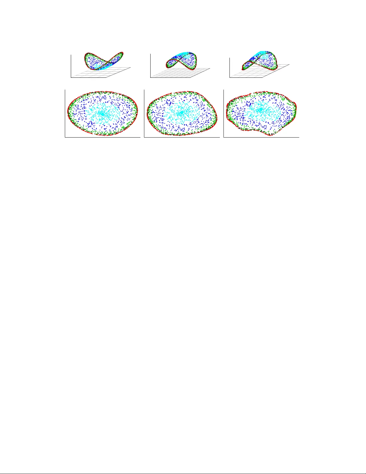
Sp ectral appro ximations in mac hine learning Darren Homrighausen Departmen t of Statistics Carnegie Mellon Univ ersity Pittsburgh, P A 15213 dhomrigh@stat.cm u.edu Daniel J. McDonald Departmen t of Statistics Carnegie Mellon Univ ersity Pittsburgh, P A 15213 danielmc@stat.cm u.edu V ersion: July 20, 2011 Abstract In man y areas of machine learning, it b ecomes necessary to find the eigen vector decomp ositions of large matrices. W e discuss tw o metho ds for reducing the computa- tional burden of sp ectral decomp ositions: the more v enerable Nystr¨ om extension and a newly in tro duced algorithm based on random pro jections. Previous work has cen tered on the ability to reconstruct the original matrix. W e argue that a more interesting and relev an t comparison is their relative p erformance in clustering and classification tasks using the approximate eigen vectors as features. W e demonstrate that p erformance is task sp ecific and dep ends on the rank of the approximation. 1 In tro duction Sp ectral Connectivit y Analysis (SCA) is a burgeoning area in statistical mac hine learn- ing. Beginning with principal components analysis (PCA) and Fisher discriminan t analysis and con tinuing with lo cally linear em b eddings [12], SCA techniques for discov ering low- dimensional metric em b eddings of the data hav e long b een a part of data analysis. More- o ver, new er tec hniques, such as Laplacian eigenmaps [2] and Hessian maps [3], similarly seek to elucidate the underlying geometry of the data by analyzing appro ximations to certain op erators and their resp ectiv e eigenfunctions. Though the tec hniques are different in man y resp ects, they share one ma jor c haracter- istic: the necessit y for the computation of a p ostiv e definite kernel and, more imp ortan tly , its sp ectrum. Unfortunately , a w ell known speed limit exists. F or a matrix W ∈ R n × n , the eigen v alue decomp osition can b e computed no faster than O ( n 3 ). On its face, this limit constrains the applicability of SCA techniques to mo derately sized problems. F ortunately , there exist metho ds in numerical linear algebra for the approximate com- putation of the sp ectrum of a matrix. Tw o such metho ds are the Nystr¨ om extension [14] and another algorithm [7] w e hav e dubbed ‘Gaussian pro jection’ for reasons that will b e- come clear. Eac h seeks to compute the eigenv ectors of a smaller matrix and then em b ed the remaining structure of the original matrix on to these eigenv ectors. These metho ds are widely used in the applied SCA communit y e.g. [6, 5]. Ho wev er, the choice as to the ap- pro ximation metho d has remained a sub jective one, largely based on the subfield of the resp ectiv e researchers. The goal of this pap er is to pro vide a careful, comprehensiv e comparison of the Nystr¨ om extension and Gaussian pro jection metho ds for appro ximating the sp ectrum of the large 1 matrices o ccuring in SCA techniques. As SCA is such a v ast field, we concen trate on one sp ecific technique, known as diffusion map from the graph Laplacian. In this technique, it is necessary to compute the sp ectrum of the Laplacian matrix L . F or a dataset with n observ ations, the matrix L is n by n , and hence the exact numerical sp ectrum quickly b ecomes imp ossible to compute. Previous w ork on a principled comparison of the Nystr¨ om extension and Gaussian pro- jection methods hav e left op en some imp ortan t questions. F or instance, [4, 13] b oth pro- vide con trasts that, while interesting, are limited in that they only consider approximation metho ds based on column sampling. F urthermore, p erformance ev aluations in the literature fo cus on reconstructing the matrix W . How ev er, in the machine learning communit y , this is rarely the appropriate metric. Generally , some or all of the eigenv ectors are used as an input to standard classification, regression, or clustering algorithms. Hence, there is a need for comparing the effect of these metho ds on the accuracy of learning mac hines. W e find that for these sorts of applications, neither Nystr¨ om nor Gaussian pro jection ac hieves uniformly b etter results. F or similar computational costs, b oth metho ds p erform w ell at manifold reconstruction. How ev er, Gaussian pro jection p erforms relativ ely p oorly in a related clustering task. Y et, it also outperforms Nystr¨ om on a standard classification task. W e also find that the choice of tuning parameters can b e easier for one metho d relative to the other dep ending on the application. The remainder of this pap er is structured as follows. In § 2 we give an ov erview of our particular choice of SCA technique — the diffusion map from the graph Laplacian — as well as introduce b oth the Nystr¨ om and the Gaussian pro jection metho ds. In § 3, we presen t our empirical results on three tas ks: low dimensional manifold recov ery , clustering, and classification. Lastly , § 4 details areas in need of further inv estigation and provides a syn thesis of our findings ab out the strengths of each appro ximation metho d. 2 Diffusion maps and sp ectral appro ximations 2.1 Diffusion map with the graph Laplacian The tec hnique in SCA that w e consider is commonly referred to as a diffusion map from the graph Laplacian. Roughly , the idea is to construct an adjacency graph on a giv en data set and then find a parameterization for the data which minimizes an ob jective function that preserves lo calit y . W e giv e a brief ov erview here. See [10] for a more comprehensiv e treatmen t. Sp ecifically , supp ose we ha v e n observ ations, x 1 , . . . , x n . Define a graph G = ( V , E , f W ) on the data suc h that V = { x 1 , . . . , x n } are the observ ations, E is the set of connections b et w een pairs of observ ations, and f W is a weigh t matrix asso ciated with every elemen t in E , corresp onding to the strength of the edge. W e mak e the common c hoice (e.g. [11, § 2.2.1]) of defining f W ij = exp  −|| x i − x j || 2 /  (1) for all 1 ≤ i, j ≤ n suc h that ( i, j ) ∈ E . F urther, w e define a normalized version of the matrix W . This can b e done either symmetrically , as W := D − 1 / 2 f W D − 1 / 2 , (2) or asymmetrically as W := D − 1 f W , (3) 2 where D := diag( P n j =1 f W 1 j , . . . , P n j =1 f W nj ). In either case, the graph Laplacian is defined to b e L := I − W . Here, I is the n by n iden tity matrix. One can show ([11, § 8.1]) that the optimal p dimensional embedding is given by the diffusion map on to eigenv ectors t wo through p + 1 of W . 1 That is, find an orthonormal matrix U and diagonal matrix Σ such that W = U Σ U > and retain the second through ( p + 1) th column of U as the features. Note that we ha v e supressed an y mention of eigen v alues in the diffusion map as they only represent rescaling in our applications and hence are irrelev ant to our conclusions. Also, L and W hav e the same eigenv ectors. In most mac hine learning scenarios, this map is created as the first step for more tra- ditional applications. It can b e used as a design (also known as a feature) matrix in clas- sification or regression. Also, it can b e used as co ordinates of the data for unsup ervised (clustering) techniques. The crucial asp ect is the need to compute the eigenv ectors of the matrix W . W e giv e an ov erview of the Nystr¨ om metho d in § 2.2 and Gaussian pro jection metho d in § 2.3 for appro ximating these eigen vectors. 2.2 Nystr¨ om As men tioned in § 1, for most cases of in terest in mac hine learning, n is large and hence the computation of the eigenv ectors of the matrix W is computationally infeasible. How ever, the Nystr¨ om extension giv es a metho d for computing the eigen vectors and eigenv alues of a smaller matrix, formed by column subsampling, and ‘extending’ them to the remaining columns. The Nystr¨ om method for approximating the eigen vectors of a matrix comes from a m uch older technique for finding a n umerical solution of in tegral equations. F or our purp oses, the Nystr¨ om method finds eigenv ectors of a reduced matrix that appro ximates the action of W . 2 Sp ecifically , c ho ose an in teger m < n and an associated index subset M ⊂ { 1 , . . . , n } =: N suc h that | M | = m to form an m × m matrix W ( m ) := W M ,M . Here our notation mimics common co ding syntax. Subsetting a matrix with a set of indices indicates the retention of those ro ws or columns. Then, we find a diagonal matrix Λ ( m ) and orthonormal matrix U ( m ) suc h that W ( m ) U ( m ) = Λ ( m ) U ( m ) . (4) These eigenv ectors are then extended to an appro ximation of the matrix U by a simple form ula. See Algorithm 1 for details and an outline of the pro cedure. Of course, c ho osing the subset M is imp ortan t. By far the most common technique is to c ho ose M by sampling m times without replacement from N . W e refer to this as the ‘uniform Nystr¨ om’ metho d. Recently , ho wev er, there has been work on making more informed and data-dep endent choices. The first w ork in this area we are aw are of can b e found in [4]. More recently , [1] prop osed sampling from a distribution formed b y all  n m  determinan ts of the possible retained matrices. This is of course not feasible, and [1] pro vides some appro ximations. W e use the scheme where instead of a uniform dra w from N , w e draw from N in prop ortion to the size of the diagonal elemen ts in W . When used, this metho d is referred to as the ‘weigh ted Nystr¨ om.’ 1 The first eigen v alue and asso ciated eigenv ector corresp ond to the trivial solution and are discarded. 2 W e consider the numerical sp ectral decomp osition of the full matrix W to b e the ‘exact’ or ‘true’ decomp osition and ignore the effects of numerical error in our nomenclature. 3 Algorithm 1 Nystr¨ om appro ximation based on subsampling Giv en an n × n matrix W and integer m < n , compute an approximation U ny s to the eigen vectors U of W . 1: Compute U ( m ) and Λ ( m ) via equation (4). 2: F orm b λ i = n m λ ( m ) i b u i = r m n 1 λ ( m ) i W N ,M u ( m ) i , where λ ( m ) i and u ( m ) i are the i th diagonal entry and i th column of Λ ( m ) and U ( m ) , resp ectiv ely . 3: Return U ny s = [ b u 1 , . . . , b u m ] 2.3 Gaussian pro jection An alternate to the Nystr¨ om metho d is a very in teresting new algorithm in tro duced in [7]. This new algorithm differs from other appro ximation techniques in that it produces, for any matrix A , a subspace of col( A ) (the column space of A ) through the action of A on a random set of linearly indep endent v ectors. This is in contrast to randomly selecting columns of A to form a subspace of col( A ) as in [4] and the Nystr¨ om metho d. This is imp ortan t as crucial features of col( A ) can b e missed by simply subsampling columns. W e include a combination of algorithms 4.1 and 5.3 from [7] in Algorithm 2 for com- pleteness. 2.4 Theoretical comparisons F or both the Nystr¨ om and the Gaussian pro jection methods, theoretical results hav e b een dev elop ed demonstrating their p erformance at forming a rank m appro ximation to W . F or the weigh ted Nystr¨ om method, [1] finds that E || W − W ny s || F ≤ || W − W m || + C n X i =1 W 2 ii (5) where W ny s is the appro ximation to W via the Nystr¨ om metho d and W m is the best rank m approximation. Likewise, for Gaussian pro jection , [7] finds that || W − W g p || F ≤ 2  1 + || Ω || σ min  δ (6) where σ min is the minim um singular v alue of Q > Ω and δ is a user defined tolerance for ho w m uch the pro jection QQ > distorts W , ie: ||  I − QQ >  W || ≤ δ. Ho wev er, these results are not generally comparable. T o the best of our kno wledge no lo wer b ounds exist showing limits to the qualit y of the approximations formed by either metho d. So theoretical comparisons of these b ounds are ill advised if not entirely meaning- less. F urthermore, it is not clear that reconstruction of the matrix W is beneficial to the mac hine learning tasks that the eigen vectors of W are used to accomplish. SCA metho ds 4 Algorithm 2 Gaussian pro jection Giv en an n × n matrix W and in teger m < n , we compute an orthonormal matrix Q that appro ximates col( W ) and use it to compute an appro ximation U g p to the eigen vectors of W , U . 1: Dra w n × m Gaussian random matrix Ω. 2: F orm Y = W Ω. 3: Construct Q , an orthonormal matrix suc h that col( Q ) = col( Y ). 4: F orm B such that B minimizes || B Q > Ω − Q > Y || 2 , ie. B is the least squares solution. 5: Compute the eigenv ector decomposition of B , ie: B = b U b Σ b U > 6: Return U g p = Q b U . often serve as dimensionality reduction to ols to create features for classification, cluster- ing, or regression metho ds. This first pass dimension reduction do es not obviate the need for doing feature selection with the computed appro ximate eigen vectors. In other words, the approximation metho ds help av oid one curse of dimensionalit y , in that large amoun ts of data incurrs the cost of a large amoun t of computations. An op en question is: can the selection of the tuning parameter m also a void another curse of dimensionality in that o ver-parameterizing the mo del leads to an increase in its prediction risk? A ma jor difference in the Nystr¨ om metho d versus the Gaussian pro jection metho d is that U g p remains an orthonormal matrix, and hence provides an orthogonal basis for col( W ). This can b e seen b y considering the output of Algorithm 2, writing u i = U g p N ,i as the i th column, and observing h u g p i , u g p j i = h Q ˆ U N ,i , Q ˆ U N ,j i = h ˆ U N ,i , ˆ U N ,j i = δ ij (7) b y the orthonomalit y of Q and ˆ U . This is in con trast to Algorithm 1 that pro duces U ny s whic h is a rotation of W N ,M b y the matrix U ( m ) . This difference has implications that need further exploration. How ev er, it does show that Gaussian pro jection pro vides a numerically sup erior set of features with whic h to do learning. 3 Exp erimen tal results In order to ev aluate the appro ximation metho ds men tioned ab o v e, we focus on three related tasks: manifold reconstruction, clustering, and classification. In the first tw o cases, w e examine simulated manifolds with and without an em b edded clustering problem. F or the classification task, w e examine the MNIST handwritten digit database [9], using diffusion maps for feature creation and supp ort vector machines (SVMs) to perform the classification. 3.1 Manifold recov ery T o in v estigate the p erformance of the t w o appro ximation metho ds through the lens of manifold recov ery , we c ho ose a standard “fishbowl” lik e ob ject. It is constructed using the 5 Fish bowl Halo and sphere Figure 1: This figure sho ws the t wo sim ulated manifolds we attempt to recov er. The fish b o wl on the left is a standard exercise in the literature, while the modified halo and ball on the righ t allows for a related clustering exercise parametric equations for an ellipsoid: u ∈ [0 , 2 π ) x = a cos u sin v v ∈ [ d, π ] y = b sin u sin v z = c cos v , where ( a, b, c ) > 0 determine the size of the ellipsoid and d ∈ [0 , π ) determines the size of the op ening. W e sample v uniformly ov er the in terv al, while u is a regularly spaced sequence of 2000 p oint s. The dominan t computational cost for the appro ximations are O ( nm 2 ) for Nystr¨ om and O ( n 2 m ) for Gaussian pro jection , w e c ho ose the parameter m so that they hav e equal dominan t cost. That is, if w e c ho ose m g p for the Gaussian pro jection metho d to b e a certain v alue, w e set m ny s for the Nystr¨ om metho d to be m ny s = √ nm g p . F or the Nystr¨ om metho d, w e take m ny s = 141 while for Gaussian pro jection, m g p = 10. The manifold reconstruction of the ellipsoid is shown in Figure 2. Both methods perform reasonably w ell. The underlying structure is well recov ered. F or this figure, the tuning parameter was set at  = 15 in all three cases. Changing it makes very little difference (  ∈ [1 , 200] yields very similar figures ov er repeated randomizations 3 ). This robustness with resp ect to tuning parameter choice is rarely the case as we will see in the next example. 4 3.2 Clustering T o create a clustering example similar to the manifold reco very problem, we remov ed the b ottom fifth of the fish b o wl and created a glob in the middle of the resulting halo. See Figure 1 for a plot of the shap e. W e consider the light blue observ ations in the middle one 3 The magnitude of the tuning parameter dep ends heavily on the intrinsic separation in the data 4 Another standard manifold recov ery example, the “swissroll”, is very sensitive to tuning parameter c hoice as well as the choice of the matrix f W . 6 Ex a c t N y s tr ö m A p p r o x i m a te SVD Figure 2: Here, the true eigen vectors along with b oth appro ximate methods demonstrate the manifold recov ery capabilities. F or equiv alent computational time, b oth metho ds p erform reasonably . The true eigenv ectors are on the left, the Nystr¨ om metho d is in the center, while the Gaussian pro jection metho d is on the right. cluster and the outer ring as a second cluster. The result is a three dimensional clustering problem for whic h linear classifiers will fail. How ever, diffusion methods yield an em b edding whic h will b e separable ev en in one dimension via linear metho ds (Figure 3, first column). The next tw o columns sho w the Nystr¨ om appro ximation with m ny s = 200 and for Gaussian pro jection with m g p = 20. W e see that Nystr¨ om provides a v ery faithful repro duction of the exact eigenv ectors. Gaussian pro jection loses muc h of the separation presen t in the other t wo methods. It is imp ortan t to keep in mind the selection of appropriate tuning parameters. Our c hoice in this example is a sub jective one, based on visual inspection. In this scenario, tun- ing parameter selection b ecomes v ery difficult, and hugely imp ortan t. Small p erturbations in the tuning parameter lead to p oor embeddings whic h not only yield p o or clustering solu- tions, but which can completely destroy the structure visible in the data alone. F urthermore, tuning parameters m ust b e selected separately for the exact as well as the t w o appro ximate metho ds with no guarantee that they will b e similar. In our particular parameterization, the exact reconstruction was successful for  ∈ [0 . 05 , 0 . 15] while the approximate metho ds required  ≈ 0 . 25. The reconstruction via Gaussian pro jection shown in Figure 3 displays the b est separation that we could ac hiev e for this computational complexity . Clearly , the Nystr¨ om metho d p erforms b etter in this case, yielding an em b edding that remains easily separable even in one dimension. 3.3 Classification A common machine learning task is to classify data based on a labelled set of training data. When all the data (training and test) are a v ailable, using the semi-sup ervised approac h of a diffusion map from the graph Laplacian is a very reasonable tec hnique for pro viding lab els for the test data. Ho wev er, this technique requires a v ery large sp ectral decomp osition as it is based on the entire dataset, b oth training and test. W e in v estigate classifying the handwritten digits found in the MNIST dataset and used in e.g. [9]. See the left panel of Figure 4 for fifteen randomly selected digits. Using SVM 7 Exact Nyström Puma Exact Nyström Puma Figure 3: Using the true eigenv ectors and with b oth approximation methods, we attempt to perform a clustering task. F or equiv alen t computational time, the Nystr¨ om metho d far outp erforms Gaussian pro jection. The true eigenv ectors are on the left, the Nys tr¨ om metho d is in the center, while the Gaussian pro jection metho d is on the right. with the (appro ximate) eigenv ectors of the graph Laplacian as features, w e attempt to classify a test set using eac h of the ab o ve describ ed appro ximation tec hniques. Though the digits are rotated and sk ewed relativ e to each other, we do not consider desk ewing as very go od classification results ha ve b een obtained using SVM without an y suc h prepro cessing (see for example [8]). W e c ho ose the smo othing parameter in the SVM via 10 fold cross- v alidation. Additionally , we c ho ose the bandwidth parameter of the diffusion map,  , by minimizing the misclassification error on the test set ov er a grid of v alues. F or small enough datasets, w e can compute the true eigenv ectors to get an idea of the efficiency loss we incurr by using each appro ximation. If we c ho ose a random dataset comprised of n train = 4000 test digits and n test = 800 training digits, then it is still feasible to calculate the true eigenv ectors of the matrix W . T able 1 displays the results with an appro ximation parameter of m = m ny s = m g p = 400. 5 W e see that the Gaussian pro jection metho d has the b est p erformance of the three considered metho ds. Additionally , as exp ected, the weigh ted Nystr¨ om metho d outp erforms the uniform Nystr¨ om, but only sligh tly . Note that the true eigenv ector misclassification rate, 5.5%, is a bit w orse than that rep orted in [8] — 1%. W e attribute this to using a muc h smaller training sample for our classification pro cedure. 5 In the manifold recov ery and clustering tasks, we are essentially in terested only in the first few eigenv ec- tors of W , so it makes sense to compare the tw o metho ds for equiv alent computational complexity . How ever in the classification task, w e wan t to create tw o comparable feature matrices which may then be regularized b y the classifier. F or this reason, it seems more natural to choose m nys = m gp . 8 Metho d # Correct n test 800 T rue eigenv ectors 756 Uniform Nystr¨ om 697 W eighted Nystr¨ om 701 Gaussian pro jection 725 T able 1: n train = 4000, m = 400 0 1000 2000 3000 4000 0.04 0.05 0.06 0.07 m Misclassification Rate (%) Gaussian Proj. Nys. Uniform Nys. Weighted Figure 4: Left: A random sample of fifteen digits from the MNIST dataset. Righ t: Mis- classification rates from running the three appro ximation metho ds on a random subset of the MNIST digits for m ∈ { 50 , 150 , 450 , 1350 , 4050 } with n train = 15000 and n test = 3000 (see text for more details). The weigh ted and uniform Nystr¨ om metho ds are very similar. The Gaussian pro jection metho d results in a w orse misclassification rate for smaller m , but its p erformance improv es mark edly for larger m . Additionally , w e ran a comparison with n train = 15000 and n test = 3000. Here computing the true eigen vectors would b egin to be truly time/resource consuming. F or each m ∈ { 50 , 150 , 450 , 1350 , 4050 } we perform the grid searc h to minimize test set misclassification for each method. W e do this a total of ten times and av erage the results to somewhat account for the randomness of each approximation method. The results app ear on the right hand side of Figure 4. W e see that again the weigh ted and uniform Nystr¨ om metho ds pro duce v ery similar misclassification rates. In terestingly , the Gaussian pro jection metho d results in a worse misclassification rate for smaller m , but its p erformance impro ves markedly for larger m . 4 Discussion In this pap er, we consider t wo main methods — the Nystr¨ om extension and another method w e dub Gaussian pro jection — for approximating the eigenv ectors of the graph Laplacian matrix W . As a metric for performance, we are in terested in ramifications of these appro x- imations in practice. That is, how do the approximations affect the efficacy of standard 9 mac hine learning tec hniques in standard machine learning tasks. Sp ecifically , we consider three common applications: manifold reconstruction, clustering, and classification. F or the last task w e additionally in vestigate a new er version of the Nystr¨ om metho d, one that allo ws for w eighted sampling of the columns of W based on the size of the diagonal elemen ts. W e find that for these sorts of applications, neither Nystr¨ om nor Gaussian pro jection ac hieves uniformly b etter results. F or similar computational costs, b oth metho ds p erform w ell at manifold reconstruction, eac h finding the lo w er dimensional structure of the fish b o wl as a deformed plane. Ho wev er, the Gaussian pro jection method reco very is somewhat distorted relative to the true eigenv ectors. In the clustering task, Gaussian pro jection p erforms relativ ely p oorly . Although the inner sphere is now linearly separable from the outer ring, the em b edding is muc h noisier than for the true eigenv ectors and the Nystr¨ om extension. Lastly , we find that the weigh ted and uniform Nystr¨ om metho ds result in nearly the same misclassification rates, with perhaps a slight edge to the w eighted v ersion. But, Gaussian pro jection outperforms both Nystr¨ om metho ds as long as m is mo derately large: ab out 10% of n . This v alue of m still provides a substantial sa vings ov er computing the true eigenv ectors. References [1] Belabbas, M., and Wolfe, P. (2009), “Sp ectral methods in machine learning and new strategies for very large datasets,” Pr o c e e dings of the National A c ademy of Scienc es , 106 (2), 369–374. [2] Belkin, M., and Niyogi, P. (2003), “Laplacian eigenmaps for dimensionality re- duction and data represen tation,” Neur al Computation , 15 (6), 1373–1396. [3] Donoho, D., and Grimes, C. (2003), “Hessian eigenmaps: locally linear embed- ding techniques for high-dimensional data,” Pr o c e e ding of the National A c ademy of Scienc es , 100 (10), 5591–5596. [4] Drineas, P., and Mahoney, M. (2005), “On the Nystr¨ om metho d for appro xi- mating a gram matrix for improv ed k ernel-based learning for high-dimensional data,” Journal of Machine L e arning R ese ar ch , 6 , 2153–2175. [5] F owlkes, C., Belongie, S., Chung, F., and Malik, J. (2004), “Sp ectral group- ing using the Nystr¨ om method,” IEEE T r ansactions on Pattern Analy sis and Machine Intel ligenc e , 26 (2), 214–225. [6] Freeman, P., Newman, J., Lee, A., Richards, J., and Schafer, C. (2009), “Photometric redshift estimation using sp ectral connectivity analysis,” Monthly No- tic es of the R oyal Astr onomic al So ciety , 398 , 2012–2021, arXiv:0906.0995 [astro- ph.CO]. [7] Halk o, N., Mar tinsson, P. G., and Tr opp, J. A. (2009), “Finding structure with randomness: Sto c hastic algorithms for constructing approximate matrix decom- p ositions,” arXiv:0909.4061 [math.NA]. [8] La uer, F., Suen, C., and Bloch, G. (2007), “A trainable feature extractor for handwritten digit recognition,” Pattern R e c o gnition , 40 (6), 1816–1824. 10 [9] LeCun, Y., Bottou, L., Bengio, Y., and Haffner, P. (1998), “Gradien t-based learning applied to do cumen t recognition,” Pr o c e e dings of the IEEE , 86 (11), 2278– 2324. [10] Lee, A., and W asserman, L. (2008a), “Spectral connectivit y analysis,” Journal of the A meric an Statistic al Asso ciation , 105 (491), 1241–1255. [11] Lee, A. B., and W asserman, L. (2008b), “Sp ectral connectivity analysis,” arXiv:0811.0121 [stat.ME]. [12] R oweis, S., and Saul, L. (2000), “Nonlinear dimensionality reduction by locally linear embedding,” Scienc e , 106 (5500), 2323–2326. [13] T al w alkar, A., Kumar, S., and R owley, H. (2008), “Large-scale manifold learn- ing,” in IEEE Confer enc e on Computer Vision and Pattern R e c o gnition, 2008 , IEEE. [14] Williams, C., and Seeger, M. (2001), “Using the Nystr¨ om method to sp eed up k ernel machines,” in A dvanc es in Neur al Information Pr o c essing Systems 13 . 11