Long-Term Energy Constraints and Power Control in Cognitive Radio Networks

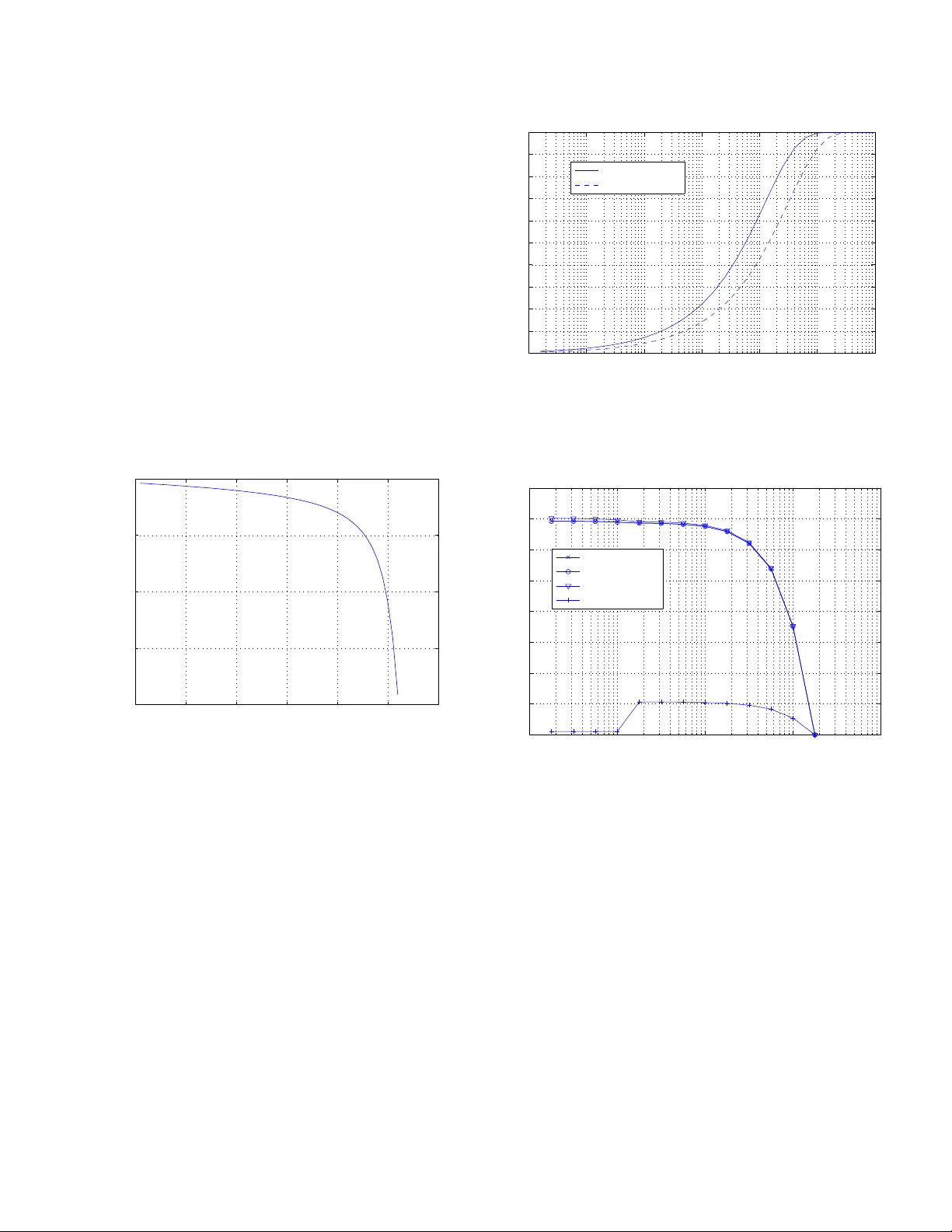
LONG-TERM ENERGY CONSTRAINTS AND PO WER CONTR OL IN COGNITIVE RADIO NETWORKS F ranc ¸ ois M ´ eriaux 1 , Y ezekael Hayel 2 , Samson Lasaulce 1 , Andr ey Garnaev 3 1 L2S - CNRS - SUPELEC - Univ Paris-Sud F-91192 Gif-sur -Yvette, France { meriaux,lasaulce } @lss .supelec.fr 2 Lab . d’Informatique d’A vignon - Univ ersit ´ e d'A vi gnon 84911 A vignon - France yezekael.hayel@univ-a vig non.fr 3 V . I.Zubov R esearch Institut e of Computational Mathematics & Control Processes St Petersb urg State Univ ersity , Russia 198504 agarnae v@rambler .ru ABSTRA CT When a long-term energy constraint is imposed to a transmitter, the av erage energy -efficienc y of a transmitter is, i n general, not max- imized by always transmitting. In a cogniti ve radio context, t his means that a secondary link can re-exp loit the non-used time-slots. In the case where the secondary link i s imposed to generate no in- terference on the primary l ink, a relev ant issue is therefore to kn ow the fraction of time-slots av ai lable to the secondary transmitter , de- pending on the system parameters. On the other hand, if t he sec- ondary transmitter is mode led as a selfish and free player choosing its powe r control policy to maximize its av erage energy-ef ficiency , resulting primary and secondary signals are not necess arily orthog- onal and st udying the corresponding Stackelber g game is relev ant to kno w the outcome of this interactiv e situation in terms of po wer control policies. Index T erms — Cognitiv e r adio, Energy-ef fi cienc y , Po wer con- trol, Primary user , S econd ary user, Stack elberg games . 1. INTRODUCTION One of the i deas of cogniti ve radio is to allow some wireless termi- nals, especially transmitters, to sense their en vironment in terms of used spectrum and to react to it dynamically . The cogniti ve radio paradigm [1] has become more and more important to the wireless community since the release of the FCC report [2]. Indeed, cogni- tiv e radio corresponds to a good way of tackling the crucial prob- lem o f spectrum co ngestion and increasing spectral ef fi cienc y . More recently , t he main actors of the telecoms industry , namely carriers, manufa cturers, and regulators hav e also realized t he importance of energy aspects i n wireless networks (see e.g., [3 ]) both at the net- work infrastructure and mobile terminal si des. There are many rea- sons for this and we wil l not pro vide them here. As far as this paper is con cerned, the goal is to st udy the influence of long-term energ y constraints (e.g., the limited battery life typically) on power control in networks where cogniti ve radios are i n volved . The performance criterion which is considered for the terminal i s deriv ed from the one introduced by Good man and Mandayam in [4]. Therein, the au- thors propose a distributed po wer control scheme for freq uency non- selectiv e block fading multiple access channels. For each block, a terminal aims a t maximizing its ind ividu al ener gy-ef ficiency na mely , the number of successfully decoded bits at the recei ver per Joule consumed at the transmitter . Although, a power control maximizing such a perfo rmance metric is called energy-ef ficient, it does not tak e into account possible long-term energy constraints. Indeed, in [4] and related references (e.g., [5][6]), the terminals always transmit, which amounts to considering no constraints on the av ailable (a ver - age) energy . The goal of t he present work is precisely to see how energy constraints modify po wer control policies in a single-user channel and in a cogniti ve radio channel. For the sake of simplic- ity , time-slotted communications are assumed. The paper is organized in two main parts. In Sec. 3 a si ngle- user chan nel is cons idered. It is shown that maximizing an av erage energy -efficienc y under a long-term energ y constraint l eads t he ter - minal to not transmit on certain blocks. The probability that the terminal does not transmit is lo wer bounded. In a setti ng where a primary transmitter has to con trol its po wer under e nergy-co nstraint, this pro bability matters since it corresponds to the fraction of av ail- able time-slots which are re-exploitable by a secondary (cognitiv e) transmitter . In Sec. 3, the single-user channel model is sufficient since the seco ndary link has to meet a z ero interference constraint (it can only exp loit non -used time-slots). I n Sec. 4, the secondary trans- mitter is assumed to be free to use all the time-slots. The technical differe nce between the primary and secondary transmitters is that the former has to choose its p ower lev el in the first place while the latter observ es this le vel and react to it. T he suited interaction model is therefore a Stackelberg game [7] where the primary and secondary transmitters are respectiv ely the leader and follower of the game. Sec. 5 prov ides numerical results which allow us to validate some deri ved results and compare the two cognitive settings (depending whether the secondary transmitter can generate no n-orthogonal sig- nals). 2. GENERAL SYSTEM MODEL In the whole paper the goal is to study a system comprising two transmitter-recei ver pairs. The signal mod el under c onsideration can be described by a frequenc y non -selectiv e b lock f ading c hannel. The signals recei ved by the two recei vers write as: y 1 = h 11 x 1 + h 21 x 2 + z 1 y 2 = h 22 x 2 + h 12 x 1 + z 2 . (1) The channel gain of t he link ij namely , h ij is assumed to be con- stant over each block or time-slot. The quantity g ij = | h ij | 2 is assumed to be a continuo us ran dom v ariable having indepe ndent re- alizations and distributed accord ing to the pro bability density func- tion φ ij ( g ij ) . The r eception noises are zero-mean complex white Gaussian noises with v ariance σ 2 . The instantaneous power of the transmitted signal x i on time-slot t is giv en by p i ( t ) = 1 N N X n =1 | x ( n ) | 2 (2) where n is the symbol index and N the number of symb ols per t ime- slot. For simplicity , transmissions are assumed to be time-slotted. T ransmitter 1 (resp. 2 ), recei ver 1 (resp. 2 ), link 11 (resp. 22 ) will be respecti vely called primary (resp. secondary ) transmitter , primary (resp. second ary) r ecei ver , and (resp. second ary) primary link. The main technica l d ifference between the primary an d the sec- ondary links is that the seconda ry transmitter can obse rve the po wer lev els chosen by the primary transmitter but the conv erse does not hold. In this paper , t wo scen arios are inv esti gated: • Scenario 1 (Sec. 3): the secon dary transmitter is i mposed to meet a zero-interference con straint on the primary link. Since the primary and sec ondary signals are orthogonal, e verything happens for the transmitter 1 as if it was transmitting o ver a single-user channel. • Scenario 2 (Sec. 4): this time, the secondary transmitter ca n use all the time-slots and not only those not exploited b y the primary l ink. P rimary and secondary signals are t herefore not orthogona l i n ge neral. In this frame work, for each time- slot, the primary transmitter chooses its power l e vel and is informed that the secondary will observe and react to it in a rational manner . A Stackelber g game formulation is proposed to study this interactiv e sit uation. 3. WHEN PRIMAR Y AND SECOND AR Y SIGNALS ARE OR T HOGON AL 3.1. Opti mal po wer control sc heme for the primary transmitter From the primary point of view , there is no interference and the signal-to-noise plus i nterference ratio (SINR) coincides with the signal-to-noise ratio (SNR): SNR( p 1 ( g 11 )) = g 11 p 1 ( g 11 ) σ 2 . (3) When using the notation p 1 ( g 11 ) instead of p 11 ( t ) we implicitly make appropriate ergodicity assumptions on g 11 . The main purpose of this section is precisely to determine the optimal control function p 1 ( g 11 ) in the sense of the long -term energy ef ficiency , which is de- fined as follo ws: u 1 ( p 1 ( g 11 )) = R 1 Z + ∞ 0 φ 11 ( g 11 ) f (SN R( p 1 ( g 11 ))) p 1 ( g 11 ) d g 11 (4) where R 1 is the transmission r ate and f is an efficienc y function representing t he packet suc cess rate f : R + → [0 , 1] . The function f is assumed to possess the following properties: 1. f is non-decre asing, C 2 differe ntiable, f (0) = 0 , lim x → + ∞ f ( x ) = 1 and there exists a unique inflection point x 0 for f . 2. f ′ is non-neg ativ e, f ′ (0) = lim x → + ∞ f ′ ( x ) = 0 . f ′ reaches its maximum for x 0 . 3. f ′′ is non-ne gativ e o ver [0 , x 0 ] , negati ve over [ x 0 , + ∞ [ . f (2) (0) = 0 , lim x → + ∞ f ′′ ( x ) = 0 − . These properties are verified by the tw o t ypical efficienc y fun ctions av ailable in the li terature: f a ( x ) =  e − a x ∀ x > 0 0 if x = 0 (5) and f M ( x ) =  1 − e − x  M ∀ x ≥ 0 . (6) The function f a , a ≥ 0 has been introduced in [8][9] and corre- sponds to t he case where the efficiency function equals one minus t he outage probability . On the other hand, f M , M ∈ N ∗ , corresponds to an empirical approximation of the packet success rate which was already used in [4]. Compared to references [4][5][6], note that the user’ s utility is the av erage energy-ef ficiency and not the instantaneous energy- efficien cy . This allo ws one to tak e into account th e follo wing ener gy constraint: T Z + ∞ 0 φ 11 ( g 11 ) p 1 ( g 11 )d g 11 ≤ E 1 (7) where T is the time-slot duration an d E 1 is the a v ailable en ergy for terminal 1 . In order to fi nd the optimal solution(s) for the power control schemes, let us consider the Lagrangian L u 1 . It writes as: L u 1 = R 1 Z + ∞ 0 φ 11 ( g 11 ) f (SN R( p 1 ( g 11 ))) p 1 ( g 11 ) d g 11 − λ ( T Z + ∞ 0 φ 11 ( g 11 ) p 1 ( g 11 )d g 11 − E 1 ) . (8) It is ready to sho w tha t the optimal instantaneous sign al-to-noise ratio (3) has to be the solution of ∂ L u 1 ∂ p 1 ( g 11 ) = 0 : xf ′ ( x ) − f ( x ) = λT σ 4 R 1 g 2 11 x 2 . (9) Solving the abov e eq uation amounts to finding the zeros of F ( x ) = xf ′ ( x ) − f ( x ) − λT σ 4 R 1 g 2 11 x 2 . W e hav e that F i s C 1 differe ntiable, F (0) = 0 , lim x → + ∞ F ( x ) = −∞ , and F ′ ( x ) = xf (2) ( x ) − 2 λT σ 4 R 1 g 2 11 x. (10) Then, ∃ ǫ, ∀ x ∈ ]0 , ǫ ] , F ′ ( x ) < 0 . Considering the sign of F ′ , giv en the particular form of f (2) , two cases ha ve to be considered. • If ∀ x , f ′′ ( x ) ≤ 2 λT σ 4 R 1 g 2 11 , F ′ is neg ativ e or null and F is de- creasing. Then 0 is the only zero for F . • If ∃ ( x 1 , x 2 ) , x 1 < x 2 st f ′′ ( x 1 ) = f ′′ ( x 2 ) = λT σ 4 R 1 g 2 11 , and F ′ non-ne gativ e over [ x 1 , x 2 ] . F decreases over [0 , x 1 ] , in- creases ov er [ x 1 , x 2 ] and decreases ov er [ x 2 , + ∞ [ . Then F may hav e zero, one or tw o zeros differen t from 0 . If F has one zero, it i s 0 and 0 is the maximum for L u 1 . If F has two zeros: 0 and x ′ 0 , L u 1 is decreasing and 0 is the maximum for L u 1 . If F has three ze ros: 0 , x ′ 1 and x ′ 2 , L u 1 decreases over [0 , x ′ 1 ] , increases ov er [ x ′ 1 , x ′ 2 ] and decreases ov er [ x ′ 2 , + ∞ [ . The maximum for L u 1 is then 0 or x 2 . Assume SN R ∗ λ E 1 ( g ) is the greatest solution of equation (9). Then an optimal po wer control schem e is giv en by: p ∗ 1 ( g 11 ) = σ 2 g 11 SNR ∗ λ E 1 ( g 11 ) (11) with SNR ∗ λ E 1 ( g 11 ) ≥ 0 . Si nce E 1 is fixed, the methodolog y con- sists in determining λ E 1 , t hen a solution of (9) is determined nu- merically . Note that λ E 1 is in bits/Joule 2 . It can be interpreted as a minimal number of bits to transmit for 1 Joule 2 . The hig her λ E 1 is, the better the chann el should be to be used. Remark (Capacity of fast fading chann els). The proposed analysis is reminiscent to the capacity determination of fast fad- ing single-user channels [10]. T wo important differenc es between this and our analysis are worth being emphasized. F irst, mathe- matically , the optimization problem under study is more general than t he one of [10]. Indeed, if one makes the particular choice f (SN R( p 1 ( g 11 ))) = p 1 log (1 + SNR( p 1 ( g 11 ))) , the optimal SNR is gi ven by SN R ∗ ( p 1 ( g 11 )) = g 11 λ E 1 σ 2 − 1 , which corresp onds to a water-filling solution (the SNR has to be non-negati ve). Second, the physical interpretation of the av erage utility is d ifferent from the fast fading case. In the fast fading case, the po wer control is updated at the symbol rate whereas in our case, i t is updated at the time-slot frequenc y namely , 1 T . Indeed, in power control problems, what is updated is the a verage po wer ov er a block or t ime-slot and assuming an average power constraint over sev eral blocks or time-slots gen- erally does not make sense. Howe ver , from an energy perspecti ve introducing an average constraint is relev ant. This comment i s a kind of subtle and characterizes our approach. 3.2. Time-slot occupancy probability As shown in the preceding section, time-slots are not used by the pri- mary link when the solution SNR ∗ λ E 1 ( g 11 ) is negati ve. Therefore, the proba bility that this ev ent occurs corresponds to the probability of ha ving a free time-slot for the secondary link. It is thus rele vant to ev aluate Pr[SNR ∗ λ E 1 ( g 11 ) ≤ 0] . At fi rst glance, exp licating this probability does not seem to be trivial. Ho wev er, one can see from the preceding section that if max f ′′ ≤ 2 λT σ 4 R 1 g 2 11 , the function F has no non-neg ativ e solutions except from 0 , in which case there is no po wer allocated to chan nel g 11 . Based on this observ ation, the fol- lo wing lower bo und arises: Pr  max f ′′ ≤ 2 λT σ 4 R 1 g 2 11  ≤ Pr[SNR ∗ λ E 1 ( g 11 ) ≤ 0] . (12) Many simulations hav e shown that this lower bound is reason- ably tight, one of them is provided in the simulation section; what matters in this paper is to sho w that the fraction of av ailable time- slots can be significant and t he proposed lo wer bou nd en sures to achiev e at least the corresponding performance. T o conclude on this point, note that in t he case where f (SNR( p 1 ( g 11 ))) = p 1 log (1 + SNR( p 1 ( g 11 ))) , the probability of having a fr ee time- slot for the secondary link can be easily expressed and is giv en by: Pr h SNR ∗ λ E 1 ( g 11 ) ≤ 0 i = 1 − e − λ E 1 σ 2 g 11 (13) where g 11 = E ( g 11 ) . A similar analysis has been made to design a Shannon-rate efficient interference ali gnment technique for static MIMO interference channels [11][12]. 4. A ST A CKELBERG FORMULA TION OF THE NON-OR T HOGONAL CASE W e assum e now that both transmitters are free to decide their powe r control policy . Howe ver , there is still hierarchy in the system in the sense that, for each time-slot, the primary transmitter has to cho ose its power le vel in the first place and the secondary transmitter (as- sumed to equipped with a cognitiv e r adio) observes this l e vel and reacts to it . This framew ork is exac tly the one of a Stack elberg game since it is assumed that the primary transmitter (called the game leader) kno ws it is o bserved by a rati onal player (the game follo wer). The SINR for the first transmitter/recei ver pair is: S I N R 1 ( p 1 , p 2 ) = p 1 g 11 σ 2 + p 2 g 21 := γ 1 , (14) where g 21 is the channel gain between transmitter 2 and receiv er 1. For the seco nd transmitter/receive r pair , the SINR is: S I N R 2 ( p 1 , p 2 ) = p 2 g 22 σ 2 + p 1 g 12 := γ 2 , (15) where g 12 is the channel gain between transmitter 1 and receiver 2. Using this relation, we hav e the po wers for transmitters 1 and 2 depending on the SINRs: p 1 = σ 2 g 11 γ 1 + γ 1 γ 2 g 21 g 22 1 − αγ 1 γ 2 , and p 2 = σ 2 g 22 γ 2 + γ 1 γ 2 g 12 g 11 1 − αγ 1 γ 2 with α = g 21 g 12 g 11 g 22 . (16) A Stackelberg e quilibrium is a vector ( p ∗ 1 , p ∗ 2 ) such that: p ∗ 1 = arg max p 1 u 1 ( p 1 , p ∗ 2 ( p 1 )) , (17) with ∀ p 1 , p ∗ 2 ( p 1 ) = arg max p 2 u 2 ( p 1 , p 2 ) . (18) Note that the abo ve expression i mplicitly assumes that the best- response of the follo wer is a singleton, which is ef fective ly the case for the problem under study . In our S tack elberg game, the utility u 2 of the secondary transmitter/recei ver p air depends on the po wer control scheme p 1 through the expres sion: ∀ p 1 , u 2 ( p 1 , p 2 ) = R 2 Z + ∞ 0 Z + ∞ 0 φ 12 ( g 12 ) φ 22 ( g 22 ) f ( p 2 g 22 σ 2 + p 1 g 12 ) p 2 d g 12 d g 22 , (19) with the ener gy constraint: T Z + ∞ 0 φ 22 ( g 22 ) p 2 d g 22 ≤ E 2 . (20) In order to determine a St ack elberg equilibrium, we first hav e to ex- press the best response of the follo wer that is, the best po wer control scheme for the secondary transmitter/receive r pair, giv en the long term po wer control sche me of the primary transmitter/receiver pair . For a gi ven p 1 ( g 12 ) , the Lagrangian L u 2 of u 2 is giv en by: L u 2 ( p 1 , p 2 , λ 2 ) = R 2 Z + ∞ 0 Z + ∞ 0 φ 12 ( g 12 ) φ 22 ( g 22 ) f ( p 2 g 22 σ 2 + p 1 g 12 ) p 2 d g 12 d g 22 − λ 2 ( T Z + ∞ 0 φ 22 ( g 22 ) p 2 d g 22 − E 2 ) . (21) Proposition 1 (Optimal SINR f or the secondary transmitter) . The secondary transmitter ha s to tune its power level such that its SINR is the gr eatest ze r o of the following equation: xf ′ ( x ) − f ( x ) = λ 2 T ( σ 2 + p 1 g 12 ) 2 R 2 g 2 22 x 2 . (22) The proof is ready and follo ws t he single-user case analysis, which is condu cted in Sec. 3. The optimal power control sche me p ∗ 2 of the secondary transmitter/receiv er pair , depending on t he power control scheme p 1 is giv en by: p ∗ 2 ( p 1 ) = σ 2 + p 1 g 12 g 22 x 2 ( p 1 ) , (23 ) where x 2 ( p 1 ) is the greatest solution of (22). No w , let us the consider the case of the primary transmitter . Proposition 2 (Optimal SINR for the primary transmitter) . The p ri- mary tra nsmitter has to tune its power le vel suc h that its SINR is the gr eatest zero of the following eq uation: xf ′ ( x ) [ 1 − αx 2 x − G ( x )] − f ( x ) = λ 1 T σ 4 R 1 g 2 11 1 + g 21 g 22 x 2 1 − αxx 2 ! 2 x 2 , with G ( x ) = αx (1 + g 12 g 11 x ) 2 x 2 (1 − αx 2 x ) 2 R 2 g 2 22 2 λ 2 T σ 4 f ′′ ( x 2 ) − (1 + g 12 g 11 x ) 2 . (24) Pr oof. The leader is optimizing his utility function u 1 taking into ac- count this best response po wer control scheme of the follo wer trans- mitter/receiv er pair . The SINR of the leader transmitter/receiv er pair , when the follo wer transmitter/receiv er pair uses his best response po wer control scheme, is gi ven by: SINR 1 ( p 1 , p ∗ 2 ( p 1 )) = p 1 g 11 σ 2 + p ∗ 2 ( p 1 ) g 21 = p 1 g 11 σ 2 (1 + g 21 g 22 x 2 ( p 1 )) + p 1 g 12 g 21 g 22 x 2 ( p 1 ) . (25) The deri vativ e of the SINR of the leader is ∂ γ 1 ∂ p 1 ( p 1 ) = g 11 σ 2 (1 + g 21 g 22 x 2 ( p 1 )) − p 1 σ 2 g 21 g 22 x ′ 2 ( p 1 ) − p 2 1 g 12 g 21 g 22 x ′ 2 ( p 1 ) ( σ 2 (1 + g 21 g 22 x 2 ( p 1 )) + p 1 g 12 g 21 g 22 x 2 ( p 1 )) 2 (26) Then we hav e p 1 ∂ γ 1 ∂ p 1 ( p 1 ) = γ 1 ( p 1 ) σ 2 (1 + g 21 g 22 x 2 ( p 1 )) − p 1 σ 2 g 21 g 22 x ′ 2 ( p 1 ) − p 2 1 g 12 g 21 g 22 x ′ 2 ( p 1 ) σ 2 (1 + g 21 g 22 x 2 ( p 1 )) + p 1 g 12 g 21 g 22 x 2 ( p 1 ) , = γ 1 ( p 1 ) 1 − p 1 g 12 g 21 g 22 x 2 ( p 1 ) + p 1 σ 2 g 21 g 22 x ′ 2 ( p 1 ) + p 2 1 g 12 g 21 g 22 x ′ 2 ( p 1 ) σ 2 (1 + g 21 g 22 x 2 ( p 1 )) + p 1 g 12 g 21 g 22 x 2 ( p 1 ) ! , = γ 1 ( p 1 ) 1 − x 2 ( p 1 ) αγ 1 ( p 1 ) − ( σ 2 + p 1 g 12 ) p 1 g 21 g 22 x ′ 2 ( p 1 ) σ 2 (1 + g 21 g 22 x 2 ( p 1 )) + p 1 g 12 g 21 g 22 x 2 ( p 1 ) ! , = γ 1 ( p 1 ) 1 − x 2 ( p 1 ) αγ 1 ( p 1 ) − σ 2 + p 1 g 12 g 12 αx ′ 2 ( p 1 ) γ 1 ( p 1 ) ! (27) T aking the exp ression of x 2 ( p 1 ) we get: x ′ 2 f ′ ( x 2 ) + x 2 x ′ 2 f ′′ ( x 2 ) − x ′ 2 f ′ ( x 2 ) = 2 λ 2 T ( σ 2 + p 1 g 12 ) R 2 g 2 22 g 12 x 2 2 + 2 λ 2 T ( σ 2 + p 1 g 12 ) 2 R 2 g 2 22 x 2 x ′ 2 , (28) which yields to: x ′ 2 f ′′ ( x 2 ) = 2 λ 2 T ( σ 2 + p 1 g 12 ) R 2 g 2 22 g 12 x 2 + 2 λ 2 T ( σ 2 + p 1 g 12 ) 2 R 2 g 2 22 x ′ 2 . (29) Then we get the deri vati ve of x 2 ( p 1 ) : x ′ 2 ( p 1 ) = 2 λ 2 T R 2 g 2 22 ( σ 2 + p 1 g 12 ) g 12 x 2 f ′′ ( x 2 ) − 2 λ 2 T R 2 g 2 22 ( σ 2 + p 1 g 12 ) 2 . (30) Then we hav e: ( σ 2 + p 1 g 12 ) x ′ 2 ( p 1 ) g 12 = 2 λ 2 T R 2 g 2 22 ( σ 2 + p 1 g 12 ) 2 x 2 f ′′ ( x 2 ) − 2 λ 2 T R 2 g 2 22 ( σ 2 + p 1 g 12 ) 2 . (3 1) T aking the e xpression of the po wer of receiver/transmitter p air 1 de- pending on both SINRs, we get: σ 2 + p 1 g 12 = σ 2 1 + g 12 g 11 γ 1 1 − αγ 1 γ 2 ! , (32) Then ( σ 2 + p 1 g 12 ) x ′ 2 ( p 1 ) g 12 = (1 + g 12 g 11 γ 1 ) 2 x 2 (1 − αγ 2 γ 1 ) 2 R 2 g 2 22 2 λ 2 T σ 4 f ′′ ( x 2 ) − (1 + g 12 g 11 γ 1 ) 2 . (33) Then we hav e: p 1 ∂ γ 1 ∂ p 1 ( p 1 ) = γ 1   1 − αx 2 γ 1 − αγ 1 (1 + g 12 g 11 γ 1 ) 2 x 2 (1 − αx 2 γ 1 ) 2 Rg 2 22 2 λ 2 T σ 4 f ′′ ( x 2 ) − (1 + g 12 g 11 γ 1 ) 2   (34) By denoting x 1 the largest so lution of this equation, the optimal po wer control scheme of the leader at the equilibrium is giv en by: p ∗ 1 g 11 σ 2 (1 + g 21 g 22 x 2 ( p ∗ 1 )) + p 1 g 12 g 21 g 22 x 2 ( p ∗ 1 ) = x 1 . (35) 5. NUMERICAL RESUL TS The following simulations are performed with the parameters: T = 10 − 3 s, R 1 = R 2 = 10 4 bits/s, σ 2 = 10 − 12 W , the channel gains g 11 and g 22 are assumed to follow a Rayleigh distr ibu tion of mean 10 − 10 , when n eeded, g 12 and g 21 are assumed t o follow a Rayleigh distribution of mean 10 − 12 and the efficienc y function used is f a , defined in Sec. 3 with a = 0 . 9 . Fig. 1 i llustrates the i nfluence of λ E on the energ y constraint in a single-user case. When λ E is lo w , the optimal po wer control scheme is to transmit most of t he time, thus the ener gy spent is high. On the contrary , when λ E increases, transmission w ill only occurs when the channel g ain is good enough , resulting in a lo w er energ y spent. After a certain threshold, the opti- mal scheme is not to transmit at all. 10 2 10 4 10 6 10 8 10 10 10 12 10 14 10 −12 10 −10 10 −8 10 −6 10 −4 λ (bits/J²) E (J) Fig. 1 . Energ y spent on duration T depending on λ E . In Fig. 2, we are in the context of Sec. 3.2. W e compute the probability per time-slot that the primary link i s not used and we compare it to its lower bound. It is interesting to note that this lower- bound is relativ ely tight to the ex act probability . Fig. 3 compares the expected util ities of Stackelberg equilibrium (Sec. 4 ) an d the orthogo nal case (Sec. 3). As we cou ld expect, the primary link of the orthogonal case offers the best util ity , but the orthogonal secondary link has the worst performance. T he leader and follower of the Stackelberg case have are much more similar in terms of performance and are very clos to the performance of the primary link which makes the Stack elberg case a very ef ficient and fair scenario for both links. Of course, like in the single-user case, after a threshold for λ , they do n ot transmit at all. 10 7 10 8 10 9 10 10 10 11 10 12 10 13 0 0.1 0.2 0.3 0.4 0.5 0.6 0.7 0.8 0.9 1 λ (bits/J²) Free time−slot probability Exact probability Lower bound Fig. 2 . Comparison of the exact probability of ha ving free time-slot with the proposed lo wer bound of this probability . 10 8 10 9 10 10 10 11 10 12 0 0.5 1 1.5 2 2.5 3 3.5 4 x 10 5 λ (bits/J²) utility (bits/J) Leader utility Follower utility Primary user Secondary user Fig. 3 . Comparison of the exp ected utilities o f Stackelber g equilib- rium and the o rthogonal cas e dep ending on λ . In this particular case, λ 1 = λ 2 = λ . In particular , Fi g. 4 sho ws the optimal po wer p rofile of the lead- ing transmitter w .r .t. the chann els gains g 11 and g 22 when λ = 10 1 0 bits/J 2 . It is clear that for lo w values of g 11 , the optimal policy is n ot to transmit. Then we distinguish two zones of interest: • when both g 11 and g 22 are good, the transmitter uses most of its powe r for a relatively high value of g 11 , • when only g 11 is good, we can see that the transmitter uses most of i ts po wer for a lower v alue of g 11 as it is not li ke ly to facing interference f rom the following t ransmitter in this zone. 6. CONCLUSION AND PERSPECTIVES In this paper, it is sho wn how a lon g-term ene rgy co nstraint modifies the behavior of a transmitter in terms of power control policy . In 10 −15 10 −10 10 −5 10 −15 10 −10 10 −5 0 0.005 0.01 0.015 g 22 g 11 Transmitting power of the leader (W) Fig. 4 . Power profile of the leading transmitter w .r .t. g 11 and g 22 in the two-player Stack elberg case. contrast wit h related work s such as [4][5][6], a transmitter d oes not alway s transmit when it is sub ject to such a constraint. This sho ws that whe n impleme nting its b est po wer control policy , a primary link does not e xploit all the a v ailable time-slots. The probability of hav- ing a free time-slot for the secondary link can be lowe r bounded in a reasonably ti ght manner an d sho wn to be non-ne gligible in general. As a second step, a scenario where the secondary link can inter- fere on the primary link is analyzed. The problem is formulated as a Stackelber g game where th e primary trans mitter is the leader and the secondary transmitter is the follo wer . An equ ilibrium in this game is sho wn to e xist for typical conditions on the efficienc y function f ( x ) . Interestingly , t he fact that the transmitters hav e a long-term energ y constraint can m ake the system more ef ficient since this incites users to interfere less; indeed simulations show the existence of a va lue of an energy budg et which maximizes t he users’ s util ities. While the po wer control schemes at the equilibrium can be determined, the corresponding equations have a drawback: the power control scheme of a given user does not only rely on the knowled ge of its indi vidual channel gain but also on the other channel gains. This sho ws the relev ance of improving the proposed work by designing more distri bu ted p ower control policies. Additionally , the prop osed scenarios inclu ded one primary link and on e secondary link. When se veral cognitiv e transm itters are present, there is a competition b e- tween the secondary transmitters for exploiting the resources left by the primary link. 7. REFERENCES [1] J. Mitola and G. Q. Maguire, “Cogniti ve radio: making soft- ware radios more personal, ” IEEE P er sonal Communications , vol. 6 , no. 4, pp. 13–18, Aug. 1999. [2] FCC, “Report of the spectrum ef ficiency working group, ” T ech. Rep., Federal Commun. Commission, USA, Nov ember 2002. [3] J. Palicot, “Cognitiv e radio: an enabling technology for the green radio communications concept, ” in I EEE International Confer ence on W ireless Communications and Mo bile Comput- ing (ICWMC) , 2009, pp. 489–49 4. [4] D. J. Goodman and N. B. M andayam, “Power control for wire- less data, ” IE EE P erson. Comm. , vol. 7, pp. 48–54, 2000. [5] F . Meshkati, M. Chiang, H. V . Poor , and S. C. S chwa rtz, “ A game-theoretic approach to energy -efficient power control in multi-carrier cdma systems, ” IEEE Journ al on Selected Ar eas in Communications , vo l. 24, no. 6, pp. 1115–1129, 2006. [6] S. Lasaulce, Y . Haye l, R. El Azouzi, and M. Debbah , “Intro- ducing hierarchy in energ y games, ” IEEE T rans. on W ir eless Comm. , vol. 8 , no. 7, pp. 3833–3843 , 2009 . [7] V . H. Stacke lberg, Marketform und Gleichge wicht , 1934. [8] E. V . Belmega and S. Lasaulce, “ An information-theoretic look at mimo energy-ef ficient communications, ” ACM Proc. of the Intl. Conf. on P erformance Evaluation Methodolo gies and T ools (V A LUETOOLS) , 2009. [9] E. V . Belmega and S. Lasaulce, “Energ y-efficient precoding for multiple-antenna termina ls, ” IEEE Tr ans. Signal Pr ocess. , vol. 5 9, no. 1, pp. 329–340, January 2011. [10] A. Goldsmith and P . V araiya, “Capacity of fading channels with channel side information, ” IE EE T ransactions on Infor- mation Theory , vol. 43, no. 6, pp. 1986–199 2, Nov . 199 7. [11] S. M. Perl aza, M. Debbah, S. Lasaulce, and J.-M. Chaufray , “Opportunistic interference alignment in MIMO interference channels, ” in IE EE 19th Intl. Symp. on P ers onal, Indo or and Mobile Radio C ommunication s (PIMRC) , Cannes, France, Sep. 2008. [12] S. M. Perl aza, H. T embin ´ e, S. Lasaulce, and M. Debbah, “Spectral efficienc y of decentralized parallel multiple access channels, ” IE EE. T rans. on Signal Processin g , 2010.