An Analytical Model for the Intercell Interference Power in the Downlink of Wireless Cellular Networks

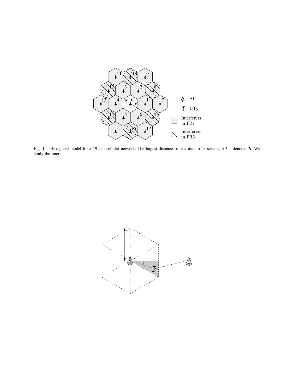
1 An Analytical Model for the Intercell Interference Po wer in the Do wnlink of W ireless Cellular Networks Benoit Pijcke, Marie Zwingelstein-Colin, Marc Gazalet, Mohamed Gharbi, Patrick Corlay Uni versit ´ e Lille Nord de France, F-59000 Lille UVHC, IEMN/DO AE, F-59313 V alenciennes CNRS, UMR 8520, F-59650 V illeneuve d’Ascq, France firstname.lastname@univ-valenciennes.fr Abstract In this paper , we propose a methodology for estimating the statistics of the intercell interference power in the downlink of a multicellular network. W e first establish an analytical expression for the probability law of the interference power when only Rayleigh multipath fading is considered. Next, focusing on a propagation en vironment where small-scale Rayleigh fading as well as lar ge-scale ef fects, including attenuation with distance and lognormal shadowing, are taken into consideration, we elaborate a semi-analytical method to b uild up the histogram of the interference power distribution. From the results obtained for this combined small- and large-scale fading context, we then de velop a statistical model for the interference po wer distribution. The interest of this model lies in the fact that it can be applied to a large range of values of the shadowing parameter . The proposed methods can also be easily extended to other types of networks. Index T erms Intercell interference po wer , statistical modeling, wireless networks, Rayleigh fading, lognormal shadowing. I . I N T RO D U C T I O N In the emerging wireless communication standards L TE-Adv anced and Mobile WiMAX, ag- gressi ve spectrum reuse is mandatory in order to achieve the increased spectral efficienc y required by IMT -Advanced for the 4th generation of standard telephony . Howe v er , since spectrum reuse comes at the expense of increased intercell interference, these standards e xplicitely require interference management as a basic system functionality [1]–[3]. The research area related to the de velopment and analysis of interference management techniques, mostly in relation with 2 the more general subject of radio ressource management, is very dynamic, as witnessed by the high number of rele v ant recent contributions in this area [4]–[10]. All these new standards use OFDMA as the modulation and the multiple access scheme. In an OFDMA system, there is no intracell interference as the users remain orthogonal, ev en through multipath channels. Howe ver , when users from different cells are present at the same time on the same subchannel, which is the case under aggressiv e frequency reuse, signals superpose, leading to some form of intercell interference. Providing statistical models of the interference power is essential to allow for an accurate e valuation of networks performances without the need for lenghtly and costly Monte Carlo simulations. The statistical characterization of the interferences has been in vestigated for a long time, under lots of different scenarios, and following sev eral approaches. The distribution of cumulated instantaneous interference power in a Rayleigh fading channel was in v estigated in [11], where an infinite number of interfering stations was considered. In [12], the interference po wer statistics is obtained analytically for the uplink and downlink of a cellular system, but in the presence of large-scale fading only . Interference modeling when considering only large- scale fading effects has also been in vestig ated in [13]–[15], where the emphasis is on finding a good approximation of the lognormal sum distrib ution. In [16], an analytical deri v ation of the probability density function (pdf) of the adjacent channel interference is deri ved for the uplink. More recently , in [17] the pdf of the do wnlink SINR was deri ved in the context of randomly located femtocells via a semi-analytical method. Other contrib utions hav e focused directly on the analysis of a particular performance measure that is influenced by intercell interference, like the probability of outage and the radio spectrum ef ficiency [18]–[20]. The analysis of interference in dense asynchronous networks, such as ad-hoc networks, is also an activ e research area, for which a deep re view of the recent developments can be found in [21], [22]. In this paper , we derive a semi-analytical methodology to estimate the statistics of the intercell interference power in a wireless cellular network, when the combined ef fects of large-scale and small-scale multipath fading are taken into consideration. Large-scale effects include attenuation with distance (path-loss) as well as lognormal shadowing, and the small-scale fading is Rayleigh distributed. W e consider a distrib uted wireless multicellular network, in both cases where power control and no po wer control is applied. The proposed methodology is semi-analytical, in that the statistical estimate of the interference power resulting from N > 1 interferers is obtained by numerical techniques from an analytically-derived interference model for one interferer . The methodology is v alid in a quite general frame work; we ha ve chosen to present it using a he xagonal network layout, although it can handle any other topology . W e validate the proposed methods by comparing the moments of the estimates to the exact moments of the distribution which can be deriv ed analytically . Using this methodology , we are able to provide a very good estimate of the pdf of the interference po wer , for dif ferent v alues of the shadowing standard deviation, σ dB . Based on these estimates, we then propose an analytical statistical model of the interference 3 po wer , based on a modified Burr distribution, which includes 5 parameters. This analytical, parameterized by σ dB , model will hopefully serve as a practical tool for the assesment and simulation of wireless cellular networks when the ef fect of shado wing is to be considered. The main contributions of this paper are as follo ws. • In the special situation where only path-loss and Rayleigh fading are considered (no shad- o wing), we deri v e a very accurate approximated analytical e xpression for the pdf and the cumulati ve distribution function (cdf) of the intercell interference power; • W e propose a semi-analytical method for the estimation of the pdf of the intercell interference po wer in a multicellular network when the combined propagation ef fects of path-loss, Rayleigh fading and lognormal shado wing are considered; • Based on this method, we deriv e an analytical model for the pdf of the intercell interference po wer by slightly modifying a Burr probability distribution. This model is parameterized by the lognormal standard de viation σ dB and its interest resides in the fact that it is valid on the whole [0 , 12] -dB range of v alues. The remainder of this paper is or ganized as follo ws. In Section II, we describe the multicell do wnlink transmission en vironment, and we provide the expression of the interference po wer for which we want to find a statistical model. In Section III, the original methodology for estimating the statistics of the interference po wer is presented. For this purpose, we examine in Section III-A the particular case where path loss and Rayleigh fast-f ading are the only fading phenomena considered. In Section III-B, we include the shadowing ef fect and we consider in the first instance the contrib ution of one interfering cell. W e then generalize to N > 1 interferers. In Section IV, we apply the proposed method to estimate the pdf of the interference po wer in a typical multicellular network, under two frequency reuse scenarios. Section V is dedicated to the parametric analytical modeling of the interference po wer . Section VI concludes the paper by summarizing the proposed methods and by presenting some perspectiv es. W e will use the follo wing notation for the rest of the paper . Non-bold letters such as x are used to denote scalar v ariables, and | x | is the magnitude of x . Bold letters like x denote vectors. W e use E { X } to denote the expectation of X . The pdf and cdf of the random variable (r .v .) X will be denoted p X ( x ) and F X ( x ) respectiv ely . I I . M U L T I C E L L D O W N L I N K T R A N S M I S S I O N M O D E L W e consider the downlink of an OFDMA-based 19-cell cellular network having the 2D hexag- onal layout depicted on Fig. 1. W e assume a unit-gain omnidirectional SISO ( single input, single output ) antenna pattern, both for the fixed access points (APs) and the mobile user terminals (UTs) which are supposed to be uniformly distributed ov er the service area. As OFDM is used for intracell communication, we assume an orthogonal transmission scheme within a cell. W e consider a synchronous discrete-time communication model in which acti ve APs at an y giv en 4 time slot send information symbols to their respective UTs o ver a shared spectral resource, which gi ves rise to an interference-limited en vironment. In this frame work, we will focus on the statistics of the so-called intercell interference power undergone by a typical UT . In this regard, we will consider UT in cell 0 (denoted UT 0 , see Fig. 1), for it is surrounded by 18 potential interferers. For UT 0 , the receiv ed signal on OFDMA subchannel ` at time slot m can be modeled as y 0 ( m, ` ) = h 0 ( m, ` ) x 0 ( m, ` ) + N X n =1 h n ( m, ` ) x n ( m, ` ) + w ( m, ` ) . Here x 0 ( m, ` ) represents the information symbol intended to UT 0 and x n ( m, ` ) , n 6 = 0 , the n th interfering symbol (this symbol is sent from AP n to its respectiv e user). The coef ficient h n ( m, ` ) denotes the instantaneous gain of the ` th (interfering) subchannel from AP n to UT 0 . Each subchannel ` is subject to additive white Gaussian noise w ( m, ` ) . In the following, we will focus without loss of generality on a single OFDMA subchannel, thereby omitting subchannel index ` in all subsequent notations. T wo frequency reuse scenarios will be considered (see Fig. 1): • the full frequency reuse pattern, denoted FR1, where all APs in the network transmit at the same time using the same frequency range ( N = 18 intercell interferers); • a partial frequency reuse pattern, denoted FR3, with reuse factor 3 ( N = 6 interferers). Each channel is assumed to be flat-fading, possibly experiencing small-scale multipath fading and/or large-scale effects. For the rest of the paper , we concentrate on the instantaneous channel power gain 1 G n ( r n ) , which is proportional to | h n ( m ) | 2 and can be expressed as a three-factor product: G n ( r n ) = G pl ,n ( r n ) G f ,n G s ,n , n = 1 , 2 , . . . , N . (1) In the abo ve equation, r n denotes the distance between UT 0 and AP n (distances r n are func- tions of UT 0 ’ s position within its cell). G pl ,n ( r n ) = K (1 /r n ) γ is the (deterministic) path loss (normalized with distance, see Appendix A), where K is a constant and γ represents the path loss exponent. The Rayleigh fading gain G f ,n is modeled by an e xponential distribution with rate parameter equal to 1 , i.e., E { G f ,n } = 1 ; we denote the corresponding pdf by p G f ,n ( x ) . The shado wing gain G s ,n is modeled by a lognormal distribution whose pdf can be written p G s ,n ( x ) = ξ √ 2 π σ dB x exp − (10 log 10 ( x ) − µ dB ) 2 2 σ 2 dB ! , x > 0 , where ξ = 10 / ln(10) [23]. Note that the importance of the shadowing phenomenon is directly related to the standard de viation σ dB . For a gi ven σ dB , the parameter µ dB is determined to ensure a unit mean shado wing gain: E { G s ,n } = 1 , which leads to µ dB = − σ 2 dB / (2 ξ ) . As r .v . ’ s G f ,n and G s ,n are independent from each other, and as E { G f ,n } = E { G s ,n } = 1 , we have, from (1), 1 As this paper will focus on power gains only , the term power will then be omitted in subsequent paragraphs. 5 E { G n ( r n ) } = G pl ,n ( r n ) , which reflects the fact that the n th interfering channel’ s Rayleigh fading and shadowing components cause the actual gain G n ( r n ) to fluctuate about its mean v alue G pl ,n ( r n ) . The total interference power undergone by UT 0 can then be written I = P N n =1 P n G n ( r n ) , where P n = E  | x n | 2  is the po wer emitted by AP n . In what follows, we consider that all APs transmit at the same power , i.e., P n = P for all n . This corresponds to, e.g., a fast-fading en vironment where no channel state information feeds back from mobile users to APs, which results in a no power control scheme where all APs transmit at the maximum power; although crude, this scheme can be seen as a lo wer bound on performance for real systems. Considering that each AP transmits at the same po wer P also applies to a more practical scenario where APs hav e access to channel state information and po wer control is associated with the opportunistic scheduling policy proposed (and pro ved to be sum-rate optimal) in [10], when the number of users per cell is high (since in this case, it can be e xpected that the channels between users scheduled at the same time and their serving APs ha ve about the same po wer gains). Thus, the interference simplifies to I = P P N n =1 G n ( r n ) . W e no w define the interfer ence gain — which will be denoted G — as being the sum of the channel power gains between the interested user and the N interferers, i.e., G = N X n =1 G n ( r n ) = N X n =1 G pl ,n ( r n ) G f ,n G s ,n . (2) (Note that G is a function of UT 0 ’ s location through the distances r n .) So, as I = P G , characterizing the interference power I is equi valent to studying the interference gain G . W e will concentrate on the latter in the subsequent sections. I I I . M E T H O D O L O G Y W e are no w interested in finding an estimate of the pdf of the random interference gain (2). Since direct calculation of the pdf does not seem possible, we aim at producing an accurate histogram for the interference gain G that will then be modeled using a specified statistical distribution. Such a histogram is constructed from a set of samples called a typical set, i.e., a discrete ensemble of values that accurately represents a random phenomenon. T raditionally (and especially in the telecommunications area), this typical set is issued from Monte Carlo simulations, which might, at first sight, produce satisfying results. Ho we ver , in a propagation en vironment that is subject to intense shado wing (i.e., for lar ge v alues of the [0 , 12] -dB range under consideration), the classical Monte Carlo method fails at producing a representativ e set of sampled gains [24], [25]. This can be explained by examining the particular distribution in v olved, for one single as well as for multiple interfering cells. A typical cdf of the interference gain (single or multiple interferers) for a high value of σ dB belongs to the class of heavy-tailed distributions [26], for which the least-frequently occuring v alues — also called rar e events — are 6 the most important ones, as a proportion of the total population, in terms of moments. A finite- time random drawing process performed on this cdf ne ver produces these rare ev ents because of their very lo w probabilities, which causes the resulting set to be not typical. Hence the need for a new approach. As will be seen in Subsection III-B2, the pdf and the cdf of the interference gain for one single interferer may be expressed in its integral form. From this expression, we propose the following two-step approach: 1) Produce a typical set of gains for one interferer using the gener alized in verse method . This method consists in generating a typical set of samples corresponding to an arbitrary continuous cdf F , and is based upon the following property: if U is a uniform [0 , 1] r .v ., then F − 1 ( U ) has cdf F ; 2) Produce a typical set for multiple interferers by adequately combining typical sets from single interferers and the Monte Carlo computational technique. A. Special case: No shadowing W e start this section by considering a propagation en vironment in which the only fading phenomenon is due to Rayleigh multipath fading. In this particular case, (1) simplifies to G n ( r n ) = G pl ,n ( r n ) G f ,n . (3) W e first note that, because of the symmetry of the network geometry , we need only study the interference power distribution for UT 0 located within one of the twelve triangular sectors depicted on Fig. 2; in the following, we will consider the grey-shaded region for illustration purposes. W e now introduce an original approximation that will help simplify further computations. W e can see that in (3), it is UT 0 ’ s random position that makes the path loss G pl ,n ( r n ) fluctuate, when the randomness of G f ,n is due to Rayleigh fading. But it is worth noting that, although both phenomena are random, path loss fluctuations differ from multipath fading in an important way : the path loss takes v alues in a finite set (related to UT 0 ’ s location within its cell) whereas the v ariations due to fading ha ve an (t heoretically) infinite dynamic range. Since pathloss fluctuations’ dynamics are very small compared to fading’ s, we propose to approximate (3) by replacing each gain G pl ,n ( r n ) by its av erage value, which leads to G n ≈ E r n { G pl ,n ( r n ) } G f ,n = E r 0 ,θ { G pl ,n ( f n ( r 0 , θ )) } G f ,n , (4) using the notation r n = f n ( r 0 , θ ) , n = 1 , 2 , ..., N , where ( r 0 , θ ) are UT 0 ’ s polar coordinates, as depicted in Fig. 2. By examining (4), we see that, under this approximation, G n does not depend on UT 0 ’ s v arying position anymore. 7 W e further note that G n , as expressed in (4), is an exponentially distributed r .v . with rate parameter 1 /λ n [27], λ n — which we call the average path loss — being defined as follows: λ n = E r 0 ,θ { G pl ,n ( f n ( r 0 , θ )) } . (5) Using (5), (4) can also be written G n ≈ λ n G f ,n , (6) and the intercell interference gain (2) can be reduced to a sum of independant (but not identically distributed) exponential r .v . ’ s: G ≈ N X n =1 λ n G f ,n . (7) G , as expressed in (7), is a r .v . whose cdf, denoted F G ( g ) , has a closed form expression av ailable in the literature [28]; it can be expressed as F G ( x ) = 1 − N X n =1 A n exp  − x λ n  , (8) where A n = λ N n N Q j =1 j 6 = n λ n − λ j , n = 1 ...N . The pdf, denoted p G ( g ) , can be easily calculated by deriving (8): p G ( x ) = N X n =1 A n λ n exp  − x λ n  . (9) In Section IV -A, it is first shown that approximation (4) is valid in the case of one single interfering cell. This consequently validates the proposed model (7) in the case of multiple interfering cells, which we show for both frequency reuse patterns FR1 and FR3. B. General case: Attenuation with distance, shadowing and multipath fading Let us now focus on characterizing the distribution of the intercell interference gain G in a propagation en vironment where Rayleigh fading as well as shadowing (due to obstacles between the transmitter and recei ver that attenuate signal po wer) are taken into account. T o the best of our knowledge, no closed form e xpression for the interference gain G exists in the literature. But, as will be seen in Section III-B2, we determine an analytical formula (under integral form) of the distrib ution of the interference gain for one interferer . Using this result, we are able to obtain a histogram for G’ s distrib ution in the presence of multiple interferers. For this purpose, we proceed in two steps: first, we compute a typical set for the interference 8 gain produced by one single interferer . As described in Section III-B2, this is done by numerical computation (from the integral-form cdf), followed by non-uniform partitioning, and then in v er- sion, of the cdf. Then we generate a typical set for N interferers using an appropriate combination of the (weighted by λ n ) typical sets of each single interferer (Section III-B3). The accuracy of the proposed method will be e v aluated in both single- and multiple-interferer cases by comparing the actual moments computed from the typical sets with the exact moments of the interference gain distribution (which can be formulated analytically , as will be seen in Section III-B1). 1) Pr eliminaries: W e begin this section by examining two important points. When taking into account multipath fading as well as shadowing as the fading ef fects in the propagation en vironment, a question arises about the v alidity of the original approximation (6). Fortunately , our approximation is being strengthened by this additional contribution due to shado wing, since this phenomenon is just another source of infinite-dynamics randomness. T aking shado wing into consideration amounts to introducing an additional term in (6) that can now be written G n ≈ λ n G f ,n G s ,n . (10) A second point pertains to the moments of both statistical distributions of G n (single interferer) and G (multiple interferers). Using approximation (10), it is shown in Appendix B that the k th- order moment of G n ’ s distrib ution has the following e xpression: E n ( G n ) k o = k ! exp  k ( k − 1) σ 2 dB 2  . (11) Computation of the k th-order moment of G ’ s distrib ution is done in Appendix C and leads to the following formula: E  G k  = k ! X a : | a | = k λ a exp σ 2 dB 2 − k + N X n =1 α 2 n !! , (12) where a = ( α 1 , α 2 , . . . , α N ) , α n ∈ N , n = 1 , 2 , . . . , N , is an N -dimensional v ector whose sum of components is written | a | = P N n =1 α n , and λ α = λ α 1 1 λ α 2 2 . . . λ α N N . So the summation in Eq (12) is taken over all sequences of non-negati v e integer indices α 1 through α N such that the sum of all α n is k . Note that the 1 st-order moment, E { G } = N X n =1 λ n , (13) is a quantity of particular interest because it is proportional to the avera ge power of the inter- ference signal. As closed form expressions of moments hav e been determined, the y may be used in ev aluating the accuracy of typical sets for both single- and multiple-interferer statistical laws. 9 2) Single interfer er: W e no w turn on to computing a typical set for the interference gain produced by one inte rferer . For con venience, the a verage path loss (5) for this single interferer is normalized to 1, i.e., λ n = 1 , so (10) reduces to G n ≈ G f ,n G s ,n . (14) As G n is the product of two independent r .v . ’ s, its cdf can be written F G n ( x ) = Z ∞ 0 p G f ,n ( u ) " Z x u 0 p G s ,n ( y ) d y # d u = Z ∞ 0 p G f ,n ( u ) F G s ,n  x u  d u, (15) where F G s ,n ( x/u ) denotes the shadowing gain’ s cdf. Recalling that G s ,n is modeled as a lognormal r .v ., we hav e, using the same notations as in Section II, F G s ,n ( x/u ) = Q  µ dB − 10 log  x u  /σ dB  , where Q ( z ) = 1 / √ 2 π R ∞ z exp ( − t 2 / 2) d t is the complementary error function of Gaussian statistics. Replacing p G f ,n ( u ) and F G s ,n ( x/u ) by their respectiv e e xpression in (15), we obtain an integral-form expression for the cdf of the intercell interference gain produced by one single interfer: F G n ( x ) = Z ∞ 0 Q 10 log 10  u x  σ dB − σ dB 2 ξ ! exp ( − u ) d u. (16) W e are now interested in generating a typical set of the interference gain G n ; we denote this typical set by S ` n , where ` is the number of elements in the set. It was mentioned in Section III that, though widely used in telecommunications, the Monte Carlo computational technique proves inef ficient for lar ge v alues of σ dB . An interesting alternative method is the generalized in verse method, for which an ` -element typical set for a gi ven distrib ution is obtained by an ` -lev el uniform partitioning, followed by in version, of the cdf. Now we know that, for large v alues of σ dB , the distribution of G n exhibits the heavy-tailed property , which means, as described before, that the least-frequently occuring v alues (i.e., the highest g ains) are the most important ones in terms of moments. Therefore, taking these highest amplitudes into consideration using the ’classical’ generalized in verse method w ould require a finer partitioning of the cdf, which would produce a typical set made up of a huge amount of elements. In order to construct a typical set with a reasonable v alue for ` , we propose to accomodate the above-mentioned method by performing a non-uniform partitioning of G n ’ s cdf, and, as high amplitudes are important in terms of moments, we proceed with a finer partitioning of the [0 , 1] segment for values close to 1 . The implementation details of the method are described on Fig. 3; they result from a good compromise between accuracy and simplicity . W e first di vide the interv al 10 [0 1] of the cdf into J intervals, numbered j = 1 , . . . , J , of dif ferent lengths: the j th interv al has a length d j = 9 × 10 − j , j = 1 , . . . , J − 1 ; the last interv al has a length d J = 10 − J to ensure P J j =1 δ j = 1 . W e next perform a P -le vel uniform partitioning on each interv al, i.e., each interv al is no w partitioned by P equally-spaced points. Finally , we in vert the partitioned cdf to obtain a typical set S ` n of cardinality ` = J × P . Also, as the proposed partitioning is non- uniform, S ` n needs to be associated a probability set: the probability of an element computed from the j th interval is δ j = d j /P . It can be sho wn (see Section IV -B) that using J = 25 interv als containing P = 900 points each — which results in a typical set that contains only ` = 25 × 900 = 22 , 500 elements 2 — guarantees that up to third-order moments deri v ed from the typical set are within 1% of the exact values for all σ dB . 3) Multiple interfer ers: W e now focus on finding an L -element typical set — denoted S L — for the interference gain G that must be computed from N typical sets S ` n , n = 1 , 2 , . . . , N . W e first note that interferer n ’ s typical set can be directly obtained by weighting each element of S ` n by its av erage path loss λ n ; we will denote interferer n ’ s typical set by λ n S ` n . Let us no w find a way to produce the ensemble S L from the typical sets λ n S ` n . Ideally , S L should be constructed by considering all combinations of the elements of the typical sets λ n S ` n , but the cardinality of the resulting set, L = ` N = ( J P ) N , would rapidly become prohibitiv e as the number N of interferers increases. T o get rid of this complexity , we point out that the above-mentioned ideal (exhausti v e) solution can also be viewed as an exhausti ve combination of intervals ( J N combinations) associated with an exhausti ve combination of elements within each interval combination ( P N combinations). And we observe that the most important part of this exhausti v e solution pertains to the combination of intervals , i.e., the combination of elements belonging to interv al j of typical set λ n S ` n with elements belonging to interv al k , k 6 = j , of typical set λ m S ` m , m 6 = n . So a way to construct a (near optimal) typical set for G could be to perform exhausti v e combinations of the intervals (as in the e xhausti ve solution), and to approximate the exhaustiv e combination of the elements within each interval combination by the following procedure: for each of the J N combinations of N P -point intervals, • Perform a random permutation of the P elements within each of the N P -point intervals 3 ; • Add up these N permuted P -point interv als to obtain one resulting P-element interval. This last P -element interv al approximates the P N -element interval that would hav e resulted from an exhausti ve combination of elements within the considered interv al combination. Now , as there are J N interv al combinations, the resulting typical set would contain J N P elements, which can still be prohibiti ve, so this second solution — which we will refer to as the near -optimal 2 T o produce moments of the same accuracy , the traditional uniform partitioning approach would require about ` = 900 × 10 25 points. 3 T wo interval combinations of the same rank j are supposed to be orthogonal because of the high number of points in each interval ( P = 900 ), which guarantees the independance of permutations. 11 solution — can not be applied as such. W e ev entually propose a novel approach which makes use of this near-optimal solution and is based on the follo wing two-step algorithm: Step 1 Apply exhausti ve combinations of intervals to a subset of M interfering links; Step 2 Perform Monte Carlo simulations for the N − M remaining links. W e no w detail the principle of the proposed method. In Step 1, we apply the near-optimal solution described abov e, but to a subset of M < N interfering links which we will call compelled links. The compelled links are chosen to hav e the highest a verage path losses ( λ 1 ≥ · · · λ M ≥ · · · λ N ) so as to minimize errors in other (non-compelled) interfering links. The exhausti v e combination of the J intervals for M compelled links obtained from the near-optimal solution thus results in one set of J M P elements. In Step 2, we b uild up a J M P -element set for each of the N − M remaining, non-compelled, links by performing J M random drawings of interv als according to the probability set { δ j } , j = 1 , 2 , . . . , J . As in the near -optimal solution, a random permutation of the elements is applied at each drawing. The ensemble of amplitudes of the intercell interference gain G — the so-called typical set S L —is then constructed by adding up these N − M + 1 sets; it is of cardinality L = J M P . Associated to S L is a probability set determined as follo ws: to each interval is associated a weight which is the product of probabilities δ k of intervals issued from compelled links (for non-compelled links, probabilities are accounted for by means of the random selection process); these weights are then normalized to obtain probabilities. Finally , the histogram of the interference gain G can be constructed from these resulting amplitude and probabiliy sets. It is important to note, howe ver , that, as a random drawing process is in v olved, a number of iterations might be needed in order for this process to con ver ge (elements of S L and associated probabilities are av eraged at each iteration). W e will call this semi-analytical technique the Monte Carlo-panel method (MCP , in short) 4 . The MCP method is illustrated on Fig. 4 for N = 4 interfering cells, M = 2 compelled links, and J = 2 interv als per typical set (these interv als — denoted A and B — hav e probabilities δ 1 = 0 . 9 and δ 2 = 0 . 1 respectiv ely , and each one of them contains P elements). Step 1 of the alogrithm is summarized in the light-grey shaded box: intervals from typical sets S ` 1 and S ` 2 (corresponding to compelled interfering links 1 and 2, and weighted by their respectiv e a verage path losses λ 1 and λ 2 ) are combined together , as described in the near-optimal solution, to obtain a set of amplitudes of cardinality 4 P representati ve of the two compelled links; associated to this set of amplitudes is a set of weights { 0 . 81 , 0 . 09 , 0 . 09 , 0 . 01 } . The dark-grey shaded box summarizes Step 2: for each non-compelled interfering link, a 4 P -element set of amplitudes is made up by 4 interv als ( A or B ) drawn according to the probability set { 0 . 9 , 0 . 1 } and applied random permutations. The typical set S L (with L = 4 P in our e xample) is then obtained by summing up together all these sets. The histogram of the interference gain G is constructed 4 The term ’panel’ refers to survey panels used by polling organizations. 12 from S 4 P and the associated probability set 5 . Note that one random permutation of the interv al (permuted intervals have been assigned the prime symbol) is performed at each (compelled or random) manipulation of an interval. Implementing the MCP method howe v er requires cautiousness. In non-compelled links, random drawings of intervals are performed based on the probability set { δ j } , j = 1 , 2 , . . . , J . In this process, lowest-probability intervals, which contain the highest interference gains, are totally ignored for two reasons. The first reason pertains to the fact that obtaining a significant frequency of appearance of such rare ev ents would require a prohibitive number of simulation runs. The second reason is due to limitations inherent to softw are simulation tools which use pseudo-random number generators to generate sequences of ’ random’ numbers belonging to a fixed set of values. In order to take into account the ignorance of the contribution of the highest interference gains of the N − M non-compelled interfering links in the probability set { δ j } , we suggest the following workaround: in these links, we intentionally make e xclusiv e use of the J , 1 ≤ J < J , first interv als, and we associate them a loaded probability set  δ 0 j  defined as follows: δ 0 j =    αδ j for 1 ≤ j ≤ J 0 for J + 1 ≤ j ≤ J (17) where α = 1 J P j =1 δ j (18) is a normalizing constant such that P J j =1 δ 0 j = 1 (using the particular non-uniform partitioning described previously , we hav e: α = 1 /  1 − 0 . 1 J  & 1 ). No w , as was mentioned before, high amplitudes play an important role in terms of moments. Although the impact of neglecting them in non-compelled links is globally limited because these links are weighted by smaller av erage path losses λ n ( n = M + 1 , . . . , N ), it has to be compensated in order to satisfy the 1 st-order moment constraint (i.e., the sampled mean has to con ver ge to the exact v alue 6 ). For this purpose, small (resp. large) amplitudes need to be underweighted (resp. ov erweighted). Thus, an underweighting multiplicativ e factor , denoted f − , is applied to amplitudes of the J first intervals of compelled links; similarly , an o verweighting multiplicativ e factor f + is applied to amplitudes of the last N − J interv als. (Computation details of factors f − and f + are giv en in Appendix D.) Let us last notice that the choice for v alues of M and J is a trade-off between dif ferents aspects: cardinality of the resulting typical set (i.e., tractable number of points), number of simulation runs and accuracy of the histogram. W e hav e determined that M = 2 and J = 3 meet all these 5 The probability set is obtained by normalizing the set of weigths. 6 W e recall that the mean E { G } is of particular importance because it is proportional to the a verage interference power . 13 requirements. I V . N U M E R I C A L R E S U LT S In this section, we present numerical results related to the different methods introduced in the preceding section. In Section IV -A, we first examine the validity of the original approximation introduced in Section III, stating that the interference g ain G n (and, consequently , G ) does not depend on the user’ s position within its cell. For this purpose, we compare the approximation of G gi ven by (6) with the ’exact’ formula (3). Then, in Section IV -B, we obtain the histogram of the interference gain G n (one single interferer) by applying the non-uniform partitioning generalized in v erse method described in III-B2. Finally , the MCP method (see III-B3) is used to build up the histogram of the interference gain for multiple interferers in Section IV -C. W e use the following simulation parameters. W e consider a system functioning at 1 GHz. W e fix the cell radius to R = 700 m, d 0 = 10 m, and the pathloss exponent to 3 . 2 , which corresponds to a typical urban en vironment, as described in the COST -231 reference model [29]. The reference distance is chosen to be equal to 2 R . A verage path losses λ n , n = 1 , 2 , . . . , N , are determined numerically using (5) and are summarized in T able I. A. No shadowing In this section, we ev aluate the proposed approximation (6) against Monte Carlo simulations performed on (3). W e first consider the contribution of one interfering cell and, in this re gard, we examine two opposite scenarios: one for which the in vestigated interferer (i.e., AP 1) produces the largest dynamic range for the intercell interference power undergone by a user in the grey- shaded triangular area of Fig. 2; the other one for which the in vestigated cell (i.e., AP 13) has the smallest dynamics. Obviously , both dynamics dif ferently impact the accuracy of our model. Note that, in both cases, the sum of interference gains (7) reduces to one exponential r .v . Modeled and simulated pdf ’ s for abov e-mentioned cases (a) and (b) are plotted in Fig. 5 and Fig. 6 respectiv ely , and the good match of the curves sho ws that the proposed method is a good approximation. W e then consider the whole set of interfering cells ( N interferers) under frequency reuse patterns FR1 and then FR3, for which results are sho wn in Fig. 7 and Fig. 8 respecti v ely . W e see that simulated and modeled probability laws (2) and (7) respectiv ely closely match for both frequency reuse patterns. W e also note that simulated and approximated curves are closer to one another for FR3 than they are for FR1. As e xplained before for the single-interferer scenario, fluctuations of actual pathlosses G pl ,n ( r n ) , n = 7 , ..., 18 , can be assumed to have about the same dynamic range, but these dynamics are smaller than those of gains G pl ,n ( r n ) , n = 1 , ..., 6 . B. Shadowing, one interferer In this section, we make use of the non-uniform partitioning generalized in v ersion method introduced in Section III-B2 to obtain a typical set for the interference gain of one interferer . 14 T able II presents the three first moments computed from typical set S ` n , as compared with the exact moments of the distribution of the interference gain G n . W e see that moments issued from the typical set are far beyond the 1% accuracy requirement. The proposed method also outperforms the Monte Carlo simulation technique, which cannot be guaranteed to con ver ge for such a small number of points. Histograms of the interference gain G n computed from typical set S ` n is illustrated on Fig. 9 for different values of σ dB . C. Shadowing, multiple interferer s W e now e valuate the MCP method de veloped in Section III-B3. W e have determined that 20 , 000 iterations of the base MCP algorithm guarantee that the 1 st-order moment computed from any typical set (whate ver σ dB v alue is considered) con v erges to its exact value (13). T able II presents the values of the 1 st-order moment of G , both exact (analytical) and approximated (computed from the typical set). W e can see that the proposed method performs very well for the whole range of σ dB v alues. Histograms of the interference gain G computed from typical sets obtained by the MCP method are illustrated on Fig. 10 (FR1 scenario) and Fig. 11 (FR3 scenario) for different v alues of σ dB . V . S TA T I S T I C A L M O D E L In Section III, we de veloped analytical and numerical methods to build up a good approx- imation of the histogram of the interference gain G . In this section, we aim at using this result to elaborate a statistical model for G , i.e., a closed form expression of the probability law , characterized by the shado wing parameter σ dB . This task is challenging in that one single parametric law is required, that is v alid for propagation en vironments which considerably v ary depending upon the shadowing phenomenon (parameter σ dB ), and that is applicable to various frequency reuse scenarios (FR1 and FR3). W e initialize the modeling process by extracting usefull information from a carefull analysis of the histograms of the interference gain G (see Fig. ’ s 10 and 11). W e first note that G is a positi ve continuous r .v . W e then observe that all curves are asymmetric, and this property is e ven more pronounced for large values of σ dB . In this case, G’ s pdf ’ s also ha ve a sharper peak and a longer, fatter tail, the last of which being a characteristic of heavy-tailed distributions (a.k.a. power distributions ), as already mentioned. Due to the strongly ske wed nature of the interference gain distribution for large σ dB ’ s, a po wer-type statistical model turns out to be suitable here. In this regard, a Pareto-like distribution seems to be a good candidate, so we focus, in first approximation, on a 3-parameter Burr-type X I I distribution [27]. The Burr distribution has a flexible shape and controllable location and scale, which makes it appealing to fit any giv en set of unimodal data that e xhibits a heavy-tail 15 behavior (e.g., it is an appropriate model for characterizing insurance claim sizes). Howe ver , as 3 parameters seem to not be sufficient to correctly characterize the interference gain distribution under those particularly tight constraints, another law is required, which of fers greater flexibility to match the whole range of σ dB v alues. Such a flexibility is provided by introducing an additional shape parameter into the Burr distrib ution, based on the follo wing property [30]: if F ( x ) is a cdf, so is ( F ( x )) η , ∀ η > 0 . Thus, we ha ve established a new Burr-based probability law , whose cdf — denoted F G ( x ) — is gi ven by F G ( x ) =      1 − 1  1 +  x β  α  k      η ,        x > 0 η > 1 α, k , β > 0 (19) where η , α and k are the shape parameters, and β is the scale parameter of the distrib ution. G’ s pdf — denoted p G ( x ) — can be easily obtained by deriving (19): p G ( x ) = η αk β  x β  α − 1  1 +  x β  α  k − 1 ! η − 1  1 +  x β  α  kη +1 . (20) W e next establish a parametric family of functions (parameterized by σ dB ) for the interference gain G by determining empirical formulas for parameters η , α , k , and β . For this purpose, we propose that all parameters (whatev er frequency scenario is considered) be modeled by the same 6-parameter function f that has the following e xpression: f ( σ dB ) = a 1 + a 2 · 1 − σ dB a 3  1 +  σ dB a 3  a 4  1 a 4 · 1 1 +  σ dB a 5  a 6 , (21) where coefficients a i , i = 1 , 2 , . . . , 6 hav e been determined empirically and are summarized in T able III. Corresponding empirical laws f , as functions of σ dB , are plotted on Fig. 12 (FR1 scenario) and Fig. 13 (FR3 scenario). The pdf ’ s of the proposed statistical model are superimposed on histograms obtained by the MCP method for different v alues of the shadowing parameter σ dB on Fig. 14 (resp. Fig. 15) for the FR1 (resp. FR3) scenario. W e no w come to the last step of our modeling process. As seen earlier , MCP-obtained histograms and the proposed Burr-based distributions closely match for the whole range of σ dB . Howe ver , care must be taken in defining the range of gains for which our model is valid. And indeed, the Burr-based statistical law needs to be truncated at a maximum v alue — denoted x t — defined in such a way that the 1 st-order 16 moment constraint holds, which we can write Z x t 0 xp G ( x ) d x = E { G } , where E { G } is the exact mean (13). As a consequence of this truncation process, a normalizing factor , A = 1 1 − P ( x > x t ) , (22) has to be incorporated in both the cdf and pdf of the elaborated model, which are then written AF G ( x ) and Ap G ( x ) respectiv ely . Regarding the empirical law x t as a function of σ dB , we also propose the same 5-parameter function for both FR1 and FR3 scenarios: x t ( σ dB ) = a 1 · exp  σ dB a 2  a 3  · exp exp −  σ dB − a 4 a 5  2 !! , (23) where coefficients a i , i = 1 , 2 , . . . , 6 ha ve been determined empirically and are summarized in T able IV. Empirical laws x t , as functions of σ dB , are plotted on Fig. 16 (FR1 scenario) and Fig. 17 (FR3 scenario). The normalizing factor may be easily computed by replacing x t by its actual value in (22). V I . C O N C L U S I O N A N D F U T U R E W O R K In this paper , we ha ve proposed a methodology to estimate the statistics of the intercell interference power in the downlink of a multicellular network. In a propagation environment subject only to path loss and multipath Rayleigh fading, we hav e established an accurate ap- proximated analytical expression for the interference po wer distrib ution. Then, considering the combined effects of path loss, lognormal shado wing and Rayleigh fading, we ha ve proposed a semi-analytical method for the estimation of the pdf of the interference po wer . Finally , we hav e de veloped a statistical model parameterized by the shado wing parameter σ dB and valid on a large range of v alues ( [0 , 12] dB). It is our hope that the methods described in this paper are suf ficiently detailed to enable the reader to apply them to other types of en vironments. A future work will pertain to impro ving the statistical interference po wer model by more closely linking the proposed model de veloped for a combined Rayleigh fading–lognormal shadowing en vironment to the ’exact’ analytical formula obtained in the case where only Rayleigh fading was considered. Another perspective is to apply the proposed methods to other wireless network topologies (e.g., ad hoc networks,...). A P P E N D I X A. Normalized channel power gain In this paper , we concentrate on the channel power gain H n ( r n ) = | h n ( m ) | 2 , where h n ( m ) is the instantaneous gain of the channel between AP n and UT 0 . H n ( r n ) can be expressed as a 17 three-factor product: H n ( r n ) = H pl ,n ( r n ) G f ,n G s ,n , (24) where r n represents the distance between UT 0 and AP n (distances r n are functions of UT 0 ’ s position within its cell), and H pl ,n ( r n ) , G f ,n and G s ,n represent the path loss, multipath Rayleigh fading and shado wing components respectiv ely . W e no w further describe these last three com- ponents. The (deterministic) path loss H pl ,n ( r n ) diminishes as the distance r n between UT 0 and AP n increases, based on the common power law [23] H pl ,n ( r n ) = K  d 0 r n  γ , (25) where K = ( c/ (4 π f d 0 )) 2 is a dimensionless constant, with c being the speed of light, f , the operating frequency , and d 0 , a reference distance for the antenna far-field; and γ represents the path loss exponent. In order to make our study independent from the antenna characteristics and the cell size, we rewrite (25) under the following form: H pl ,n ( r n ) = K  d 0 d ref  γ  d ref r n  γ , (26) where d ref is a reference distance, and we introduce the normalized path loss G pl ,n ( r n ) , defined as follows: G pl ,n ( r n ) =  d ref r n  γ . (27) From (26) and (27), we establish the following relationship: G pl ,n ( r n ) = 1 K  d 0 d ref  γ H pl ,n ( r n ) . (28) In a similar manner , we define the normalized instantaneous power gain G n ( r n ) as follows: G n ( r n ) = 1 K  d 0 d ref  γ H n ( r n ) = G pl ,n ( r n ) G f ,n G s ,n , (29) where (29) deriv es from (24) and (28). 18 B. Computation of moments for one interfer er W e find the closed form expression of the k th-order moment E n ( G n ) k o of the statistical distribution of the interference gain G n (one interfering cell). W e ha ve: E n ( G n ) k o = E n ( G f ,n G s ,n ) k o = E n ( G f ,n ) k o E n ( G s ,n ) k o , (30) where (30) follows from the independance property of the r .v . ’ s G f ,n and G s ,n . As G f ,n is exponentially distrib uted with unit mean, its k th-order moment is giv en by: E n ( G f ,n ) k o = k ! (31) As for G s ,n , it has a lognormal distrib ution with parameters − σ dB / 2 and σ dB ; its ra w moment can be written: E n ( G s ,n ) k o = exp  k ( k − 1) σ 2 dB 2  . (32) Replacing (31) and (32) in (30) leads to (11). C. Computation of moments for multiple interfer ers W e establish the analytical formula of the k th-order moment E  G k  of the statistical dis- tribution of the interference gain G (multiple interferers). Using approximation (10), we can write: E  G k  = E    N X n =1 λ n G f ,n G s ,n ! k    = E    X a : | a | = k k ! a ! Z a    , (33) where the following notation is used: • a = ( α 1 , α 2 , . . . , α N ) , α n ∈ N , n = 1 , 2 , . . . , N , is an N -dimensional vector whose sum of components is | a | = N X n =1 α n ; • the multifactorial a ! is such that a ! = N Y n =1 ( α n !) ; • the variable Z a is defined as follo ws: Z a = ( λ 1 G f , 1 G s , 1 ) α 1 ( λ 2 G f , 2 G s , 2 ) α 2 · · · ( λ N G f ,N G s ,N ) α N . 19 Using (30), we can further dev elop (33), which giv es (12). D. Computation of corr ection factors W e determine the correction factors used in the MCP method described in Section III-B3. Recall that the technique consists, for non-compelled links, in randomly selecting intervals from a subset containing only the J highest-probability (i.e., smallest-amplitude) intervals. But, as high-amplitude intervals nev er appear in this random process, small amplitudes get overweighted in non-compelled links, which must be compensated in compelled links, where small (resp. lar ge) amplitudes need to be underweighted (resp. overweighted), in such a way that the 1 st-order sampled moment con v erges to its exact value. Thus, in order to satisfy the mean constraint, an underweighting multiplicati ve factor , denoted f − , is applied to amplitudes of the J first intervals of compelled links; similarly , an ov erweighting multiplicativ e factor f + is applied to amplitudes of the last N − J interv als. W e no w compute these two correction factors. Let us first see how each interfering link contributes to the 1 st-order moment of the intercell interference gain G . For each compelled link n , n = 1 , . . . , M , we can write 7 : E { G n } = J X j =1 δ j g j = J X j =1 δ j g j | {z } A + J X j = J +1 δ j g j | {z } B = 1 , where G n = G f ,n G s ,n (approximation (14), with λ n = 1 ), and, by construction of the typical set S ` n , A + B = 1 , ∀ σ dB . For each non-compelled link n , n = M + 1 , . . . , N , G n ’ s mean is E { G n } = J X j =1 δ 0 j g j < 1 , where the probability set  δ 0 j  is given by (17). So, if no correction factors are introduced, the contribution of all (compelled and non-compelled) links to the intercell interference gain G giv es 7 Note that, for the sake of simplification, each P -element interval is reduced to its center of mass — denoted g j . 20 the following mean: E { G } = M X n =1 λ n E { G n } | {z } =1 + N X n = M +1 λ n E { G n } | {z } < 1 < N X n =1 λ n , where N X n =1 λ n = A N X n =1 λ n + B N X n =1 λ n (34) is the exact mean (13). Let us now introduce the correction factors f − and f + into compelled links, as described pre viously . G ’ s 1 st-order moment — denoted E cor { G } — then becomes: E cor { G } = M X n =1 λ n J X j =1 δ j f − g j + J X j = J +1 δ j f + g j ! + N X n = M +1 λ n J X j =1 αδ j g j = M X n =1 λ n  Af − + B f +  + N X n = M +1 λ n αA = A f − M X n =1 λ n + α N X n = M +1 λ n ! + B f + M X n =1 λ n . (35) In order for both exact and actual means to be equi v alent (i.e., (34) ≡ (35)), we need to solve the follo wing system:              f − M X n =1 λ n + α N X n = M +1 λ n = N X n =1 λ n f + M X n =1 λ n = N X n =1 λ n which leads to f − = 1 − ( α − 1) N P n = M +1 λ n M P n =1 λ n (36) f + = 1 + N P n = M +1 λ n M P n =1 λ n . (37) Note that we hav e f + > 1 and, as α & 1 , f − . 1 . 21 R E F E R E N C E S [1] N. Himayat, S. T al war , A. Rao, and R. Soni, “Interference management for 4G cellular standards [W iMAX/L TE UPD A TE], ” IEEE Communications Magazine , vol. 48, no. 8, pp. 86–92, August 2010. [2] IEEE 802.16m System Description Documents (SDD) 0034r3 , IEEE Std., Rev . r3, June 2010. [Online]. A vailable: http://www .ieee802.or g/16/tgm/docs/80216m- 09 0034r3.zip [3] TS 300 Evolved Universal Terrestrial Radio Access (E-UTRA) and Evolved Universal Terr estrial Radio Access Networks (E-UTRAN); overall description; Stag e 2 , 3GPP Std., 2010. [4] Y . J. Choi, N. Prasad, and S. Rangarajan, “Intercell radio ressource management through network coordination for IMT- advanced systems, ” EURASIP Journal on W ir eless Communications and Networking , vol. 2010, no. 4, February 2010. [5] G. Boudreau, J. Panicker , G. Ning, R. Chang, W . Neng, and S. Vrzic, “Interference coordination and cancellation for 4G networks, ” IEEE Communications Magazine , vol. 47, pp. 74–81, April 2009. [6] H. Zhang, X. D. Xu, J. Y . Li, X. F . T ao, T . Svensson, and C. Botella, “Performance of power control in inter-cell interference coordination for frequency reuse, ” The J ournal of China Universities of P osts and T elecommunications , vol. 17, pp. 37–43, February 2010. [7] A. Hernandez, I. Guio, and A. V aldovinos, “Radio ressource allocation for interference management in mobile broadband OFDMA based networks, ” W ireless Communications Mobile Computing , v ol. 10, pp. 1409–1430, November 2010. [8] M. S. Kang and B. C. Jung, “Decentralized intercell coordination in uplink cellular network using adaptive sub-band exclusion, ” in Pr oc. of IEEE W ireless Communications and Networking Confer ence, WCNC’09 , April 2009, pp. 1–5. [9] D. Gesbert, S. Hanly , H. Huang, S. Shamai, O. Simeone, and W . Y u, “Multi-cell MIMO cooperativ e networks: A new look at interference, ” IEEE Journal of Selected Areas in Communications , vol. 28, no. 9, pp. 1380–1408, December 2010. [10] S. G. Kiani and D. Gesbert, “Optimal and distributed scheduling for multicell capacity maximization, ” IEEE T ransactions on W ir eless Communications , vol. 7, pp. 288–297, January 2008. [11] R. Mathar and J. Mattfeldt, “On the distribution of cumulated interference power in rayleigh fading channels, ” W ir eless Networks , vol. 1, no. 1, pp. 31–36, January 1995. [12] M. Zorzi, “On the analytical computation of the interference statistics with applications to the performance evaluation of mobile radio systems, ” IEEE T ransactions on Communications , vol. 45, no. 1, January 1997. [13] N. C. Beaulieu and X. Qiang, “ An optimal lognormal approximation to lognormal sum distributions, ” IEEE T ransactions on V ehicular T echnology , vol. 53, no. 2, pp. 479–489, March 2004. [14] J. C. S. Santos Filho, Y acoub, M. D., and P . Cardieri, “Highly accurate range-adaptiv e lognormal approximation to lognormal sum distributions, ” Electr onic Letters , vol. 42, no. 6, pp. 361–363, March 2006. [15] S. S. Szyszkowicz, “Interference in cellular networks: sum of log-normal modeling, ” Ph.D. dissertation, 2007. [16] H. Haas and S. McLaughlin, “ A deriv ation of the pdf of adjacent channel interference in a cellular system, ” IEEE Communications Letters , vol. 8, no. 2, pp. 102–104, February 2004. [17] K. W . Sung, H. Haas, and S. McLaughlin, “ A semianalytical PDF of do wnlink SINR for femtocell networks, ” EURASIP Journal on W ir eless Communications and Networking , v ol. 2010, no. 5, January 2010. [18] R. Prasad and A. K egel, “Improv ed assesment of interference limits in cellular radio performance, ” IEEE T ransactions on V ehicular T echnology , vol. 40, no. 2, pp. 412–419, May 1991. [19] F . Berggren and S. B. Slimane, “ A simple bound on the outage probability with lognormally distributed interfers, ” IEEE Communications Letters , vol. 8, no. 5, pp. 271–273, May 2004. [20] M. Pratesi, F . Santucci, and F . Graziosi, “Generalized moment matching for the linear combination of lognormal R Vs - Application to the outage analysis in wireless systems, ” in Pr oc. of IEEE International Symposium on P ersonal, Indoor and Mobile Radio Communications , September 2006, pp. 1–5. [21] M. Haenggi and R. K. Ganti, “Interference in large wireless networks, ” F oundations and T r ends in Networking , vol. 3, no. 2, pp. 127–248, 2008. [22] P . Cardieri, “Modeling interference in wireless ad-hoc networks, ” IEEE Communications Surveys and T utorials , vol. 12, no. 4, pp. 551–572, 2010. [23] A. Goldsmith, W ireless Communications . Cambridge Univ ersity Press, 2005. [24] Z. Huang and P . Shahab uddin, “ A unified approach for finite-dimensional, rare-e vent monte carlo simulation, ” in Pr oceedings of the 36th Conference on W inter Simulation , 2004, pp. 1616–1624. 22 T ABLE I A V E R AG E P A T H L O S S E S λ n , n = 1 , 2 , . . . , N , D E FI N E D B Y (6) , I N D E C R E A S I N G O R D E R O F I M P O RTA N C E . E AC H I N D E X m O F C O L U M N AP m C O R R E S P O N D S T O I N D E X O F A VE R A G E PA T H L O S S λ n ( n 6 = m , I N G E N E R A L ) . FR 1 ( N = 18 ) FR 3 ( N = 6 ) n λ n AP m n λ n AP m 1 6 . 467 1 1 0 . 568 8 2 3 . 588 2 2 0 . 426 18 3 1 . 708 6 3 0 . 307 10 4 1 . 069 3 4 0 . 219 16 5 0 . 767 5 5 0 . 178 12 6 0 . 663 4 6 0 . 158 14 7 0 . 568 8 8 0 . 426 18 9 0 . 316 7 10 0 . 307 10 11 0 . 260 9 12 0 . 219 16 13 0 . 188 17 14 0 . 178 12 15 0 . 158 14 16 0 . 145 11 17 0 . 118 15 18 0 . 107 13 [25] S. Asmussen, K. Binswanger , and B. Hojgaard, “Rare ev ent simulation for hea vy-tailed distributions, ” Bernouilli , vol. 6, no. 2, pp. 303–322, 2000. [26] N. Markovitch, Nonparametric Analysis of Univariate Heavy-T ailed Data: Research and Practice , J. W iley , Ed. John W iley & Sons, 2007. [27] N. L. Johnson, S. Samuel K otz, and N. Balakrishnan, Continuous Univariate Distributions , 2nd ed. John Wile y & Sons, 1994, vol. 1. [28] S. V . Amari and R. B. Misra, “Closed-form expressions for distribution of sum of exponential random variables, ” IEEE T ransactions on Reliability , vol. 46, no. 4, pp. 519–522, December 1997. [29] European Cooperative in the Field of Science and T echnical Research EUR O-COST 231, “Urban transmission loss models for mobile radio in the 900 and 1800 MHz bands, ” The Hague, T ech. Rep., September 1991, rev . 2. [30] R. D. Gupta and D. Kundu, “Introduction of shape/ske wness parameter(s) in a probability distribution, ” J ournal of Pr obability and Statistical Science , vol. 7, no. 2, pp. 153–171, August 2009. 23 T ABLE II E X AC T A N D A P P R OX I M A T E D M O M E N T S F O R O N E S I N G L E I N T E R F E R E R A N D F O R M U LT I P L E I N T E R F E R E R S . no shadowing ( σ dB = 0 dB) intense shadowing ( σ dB = 12 dB) exact approximated e xact approximated E { ( G n ) } 1 1 1 0 . 990 E  ( G n ) 2  2 2 4 . 138 · 10 3 1 . 119 · 10 3 E  ( G n ) 3  6 6 53 . 127 · 10 9 13 . 246 · 10 6 E { ( G ) } (FR1) 17 . 25 17 . 10 17 . 25 17 . 08 E { ( G ) } (FR3) 1 . 857 1 . 857 1 . 857 1 . 855 T ABLE III C O E FFI C I E N T S a i , i = 1 , 2 , . . . , 6 , O F T H E E M P I R I C A L L AW S O F PA R A M E T E R S η , α , k , A N D β ( F R 1 A N D F R 3 S C E N A R I O S ) . FR 1 FR 3 a 1 a 2 a 3 a 4 a 5 a 6 a 1 a 2 a 3 a 4 a 5 a 6 η 4 0 1 1 1 1 0 1 1 1 1 1 α 0 . 93 0 . 87 65 1 7 . 2 3 . 2 0 . 38 0 . 94 39 . 90 2 . 00 8 . 30 3 . 00 k 0 . 65 2 . 18 3 . 3 0 . 39 4 . 75 2 . 06 0 12 . 70 2 . 35 2 . 07 11 . 00 6 . 47 β 0 . 04 16 . 44 13 . 45 9 6 . 35 2 . 56 1 . 81 24 . 35 3 . 60 2 . 77 1 . 77 1 . 31 T ABLE IV C O E FFI C I E N T S a i , i = 1 , 2 , . . . , 6 , O F T H E E M P I R I C A L L AW S O F PA R A M E T E R x t ( F R 1 A N D F R 3 S C E N A R I O S ) . a 1 a 2 a 3 a 4 a 5 FR 1 61 . 56 6 . 06 1 . 84 5 . 27 2 . 51 FR 3 1 . 71 5 . 10 1 . 89 6 . 40 2 . 30 24 0000 0000 0000 0000 1111 1111 1111 1111 0000 0000 0000 0000 1111 1111 1111 1111 000 000 000 000 111 111 111 111 000 000 000 000 111 111 111 111 0000 0000 0000 0000 1111 1111 1111 1111 0000 0000 0000 0000 1111 1111 1111 1111 0 0 1 1 9 10 11 12 3 2 8 13 4 0 1 7 18 6 5 14 15 16 17 R AP UT 0 Interferers in FR1 Interferers in FR3 Fig. 1. Hexagonal model for a 19-cell cellular network. The largest distance from a user to its serving AP is denoted R . W e study the interference power undergone by the mobile receiver UT 0 in the central cell (numbered 0 ). UT 0 r n r 0 θ AP n R Fig. 2. Because of the particular symmetry of the network geometry , we need only study the interference gain distribution for a user located within one the twelve dashed triangular areas. For illustration purposes, we will consider the grey-shaded sector . 25 0 1 δ 3 = 10 − 2 δ 1 = 9 · 10 − 1 ∆ i = 10 − 2 δ 2 = 9 · 10 − 2 ∆ i = 10 − 1 (a) (b) (1 ≤ i ≤ P ) ( P + 1 ≤ i ≤ 2 P ) 0 . 99 0 . 98 0 . 97 0 . 96 0 . 95 0 . 94 0 . 93 0 . 92 0 . 91 0 . 90 0 . 9 0 . 8 0 . 7 0 . 6 0 . 5 0 . 4 0 . 3 0 . 2 0 . 1 Fig. 3. Illustration of the general inv erse method with non-uniform partitioning ( J = 3 , P = 9 ): (a) non-uniform partitioning of the [0 , 1] segment; (b) uniform partitioning of interval I 2 . 26 random drawings and permutations δ 1 δ 2 λ 1 B 0 λ 1 A 0 interferer 1 (compelled) δ 1 δ 2 λ 2 A 0 λ 2 B 0 interferer 2 (compelled) δ 1 δ 2 A B typical set S ` n amplitudes probabilities δ 2 2 δ 2 δ 1 δ 1 δ 2 δ 2 1 δ 2 2 δ 2 δ 1 δ 1 δ 2 δ 2 1 . λ 1 A 0 + λ 2 B 0 λ 1 B 0 + λ 2 B 0 λ 1 B 0 + λ 2 A 0 λ 1 A 0 + λ 2 A 0 λ 3 A 0 λ 3 A 0 λ 3 B 0 λ 3 A 0 λ 1 A 0 + λ 2 A 0 λ 1 A 0 + λ 2 B 0 λ 1 B 0 + λ 2 A 0 λ 1 B 0 + λ 2 B 0 + λ 3 A 0 + λ 4 A 0 + λ 3 B 0 + λ 4 A 0 + λ 3 A 0 + λ 4 A 0 + λ 3 A 0 + λ 4 A 0 interferers 1 and 2 (compelled) λ 4 A 0 λ 4 A 0 λ 4 A 0 λ 4 A 0 interferer 3 interferer 4 STEP 1 STEP 2 typical set S L Fig. 4. Illustration of the MCP method for N = 4 interfering cells, M = 2 compelled links, and J = 2 intervals per link (denoted A and B , with respective probabilities δ 1 and δ 2 ). Each A 0 (resp. B 0 ) represents one random permutation of A (resp. B ). 27 simulation model 40 0 10 20 30 50 g 0 . 05 0 . 10 0 . 15 p G AP 1 ( g ) Fig. 5. Simulated vs. modeled pdf of the intercell interference power with no shadowing when AP 1 is the only interferer . Since AP 1 produces the largest dynamics for the interference po wer undergone by a user in the grey-shaded sector of Fig. 2 with only one interfering cell, these curves correspond to the worst-case scenario for validating our approximation. simulation model 0 g 10 2 4 6 8 0 . 1 0 . 2 0 . 3 0 . 4 0 . 5 0 . 6 p G AP 13 ( g ) Fig. 6. Simulated vs. modeled pdf of the intercell interference power with no shadowing when AP 13 is the only interferer . AP 13 produces the smallest dynamics for the interference power undergone by a user in the grey-shaded sector of Fig. 2 with only one interfering cell (best match for our model). 28 simulation model 0 g 10 60 50 40 30 20 p G FR 1 ( g ) 0 . 07 0 . 06 0 . 05 0 . 04 0 . 03 0 . 02 0 . 01 Fig. 7. Simulated vs. modeled pdf of the intercell interference power G for frequency reuse pattern FR1. simulation model 0 g 1 2 3 4 5 6 p G FR 3 ( g ) 0 . 5 0 . 4 0 . 3 0 . 2 0 . 1 Fig. 8. Simulated vs. modeled pdf of the intercell interference power G for frequency reuse pattern FR3. 29 1 σ dB = 0 σ dB % 0 2 σ dB = 4 σ dB = 12 · · · g p G n ( g ) E { G n } = 1 Fig. 9. Histograms of the interference gain G n (one interferer) for different values of σ dB . 30 0 10 1 2 σ dB = 12 σ dB % g σ dB = 0 p G ( g ) E { G } = 17 . 25 Fig. 10. Histograms of the interference gain G obtained by the MCP method (FR1 scenario). 31 0 4 3 2 1 1 σ dB % σ dB = 12 σ dB = 0 g p G ( g ) E { G } = 1 . 857 Fig. 11. Histograms of the interference gain G obtained by the MCP method (FR3 scenario). 32 6 12 0 σ dB 6 12 0 σ dB 6 12 0 σ dB 6 12 0 σ dB α β k 4 3 2 1 5 10 15 20 0 . 5 . η 3 . 0 2 . 5 2 . 0 1 . 5 1 . 0 2 . 0 1 . 5 1 . 0 0 . 5 Fig. 12. Empirical laws η , α , k , and β as functions of σ dB (FR1 scenario). 33 6 12 0 σ dB 6 12 0 σ dB 6 12 0 σ dB 6 12 0 σ dB α β k 4 1 2 3 . 12 10 8 6 4 2 10 5 15 20 25 η 0 . 5 1 . 0 1 . 5 Fig. 13. Empirical laws η , α , k , and β as functions of σ dB (FR3 scenario). 34 0 10 1 2 σ dB = 12 σ dB % g σ dB = 0 simulation E { G } = 17 . 25 model p G ( g ) Fig. 14. Comparison of MCP histograms and modeled cdf of the interference gain G for σ dB = 0 , 3 , 6 , 9 , 12 (FR1 scenario). 35 0 4 3 2 1 1 σ dB % σ dB = 12 σ dB = 0 simulation g p G ( g ) model E { G } = 1 . 857 Fig. 15. Comparison of MCP histograms and modeled cdf of the interference gain G for σ dB = 0 , 3 , 6 , 9 , 12 (FR3 scenario). 36 0 6 12 σ dB 1 , 000 2 , 000 x t Fig. 16. T runcation gain x t as a function of σ dB (FR1 scenario). 0 6 12 σ dB x t 800 400 Fig. 17. T runcation gain x t as a function of σ dB (FR3 scenario).