Metrics of Risk Associated with Defects Rediscovery

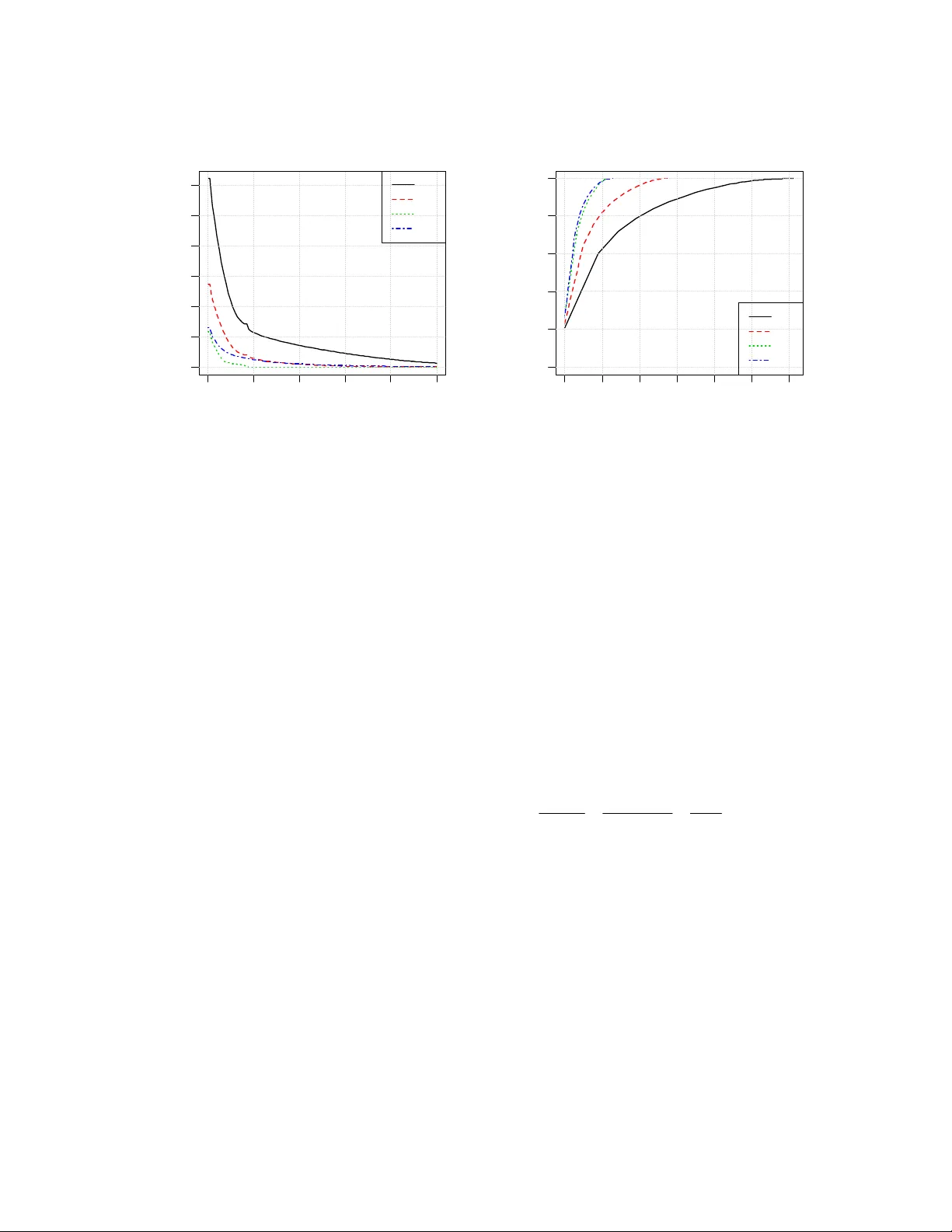
1 Metrics of Risk Associated with Defects Rediscovery A.V. Miranskyy a , M. Davison b , M. Reesor c a IBM Canada Ltd., To ron to, ON, Can ada Department of { a,b,c Applied Mathematics | b Statistical & Actu arial Sciences | b Richard Ivey School of Business}, Univers ity of Western Ontario, Canada a andriy@ca.ibm.com , { b mdavison | c mreesor}@uwo.ca Abstract Software de fects rediscovered by a large num ber of custom ers affect various st akeholders and may: 1) hint at gaps in a software m anufacturer’s Qual- ity Assurance (QA) processe s , 2 ) l e a d t o a n o v e r - load of a softwa re manufacturer’ s support and maintenance teams, and 3) consum e customers’ resources, leading to a loss of reputatio n and a decrease in sales. Quantifying risk associated with the redis- covery of defects can help all of these stake- holders. In this chapter we present a set of metrics needed to quantify th e risks. The metrics are de- signed to help: 1) the QA tea m to assess their processes; 2) the support and maintenan ce teams to allocate their res ources; and 3) th e customer s to assess the risk associated with using the software product. The paper include s a validation case study which app lies the risk metrics to industrial data. To calculate the metrics we use mathemati- cal instruments like the h eavy-tailed Kappa distri- bution an d the G/M/ k queuing m odel. 1 Intr oduction During in-hou se testing of a software produ ct, the Quality Assurance (QA) team attempts to remove defects injected during so ft ware development. It is impossible to remove all defects before ship- ping the softw are product. As cust omers use the product, they discover defects that “esca ped” the QA team. After receiving a defect report the soft- ware provi der’s mai ntenance team prepa res and makes available a fix. A discovered defe ct is sometimes rediscovered by an other custom er. Copyright © 2011 This rediscov ery could occur beca use another customer finds the de fect before the fix is avail- able or has not been inst alled. A defects relating to rarely used software features will be rediscov- ered infrequently. Howeve r, a defect relating to popular and e xtensively use d features may affect a significant fraction of customers. Frequently rediscovered defect s (affecting many customers) can ca use an avalanc he of re- quests, defined as a large number of re quests for fixes from multiple customers within a short time- frame. Because differe nt so ftware versions are run on differe nt software and hardware platfo rms, each customer may require a different fix. An avalanche has significa nt conseque nces: support personnel will experience a h eavy volume of support requests and the mainten ance team will need to prepare a large number of special builds while customers await t he official fix. On the other side, t he custom ers’ system adm inistrators will need to spend time assessing the fix’s risk and distributing it to their systems. An inordinate number of de fects may dimini sh the provider’s reputation and result in decreased software sales. Frequent redis covery of a defect sugge sts that one or more common functionalities were not properly tested. Analysis of such defects is im por- tant to identify g aps in QA processes to prevent the future escape of similar defects. Defect risk analysis is therefore important for software m anufacturers and custom ers alike. We propose a set of quantitative risk metrics which can be used to assist: • The support team’s assessment of the po- tential number of repeated calls on the same subject, hel ping in person nel alloca- tion; • The maintenance tea m’s estimation of the potential number of repeate d special builds, 2 assisting in reso urce allocation of team members; • The QA team’s assessment of trends in fre - quently redi scovered defect s on release-to- release basis. If the tre nd shows increased defect rediscovery, QA proc esses must be improved. The resulting strategy to clos e testing pr ocess gaps can be derived by root cause analysis of frequently redisc overed defects; • The customer’s assessment of the risks as- sociated with software produc t use. We present a validation case stud y showing applicability of these new metrics to an industrial dataset of defects rediscove ry. In order to model the data we derive a com pound Kappa di stribution and use the G/M/k queu eing model. Section 2 of this paper revie ws relevant wor k. Motivation for the metrics applications is de- scribed in Sect ion 3 with thei r formal defini tions deferred until Section 4. Section 5 provid es a validation case study, showing application of the metrics to the industrial data. Finally, Sectio n 6 concludes the paper. 2 Related Resear ch The paper’s main co ntribution is a set of metrics for assessing defect re discovery risks. T he follow- ing metri cs have been form ulated by other a uthors: the number of redisc overies per defect [ 1], the time interval between first and last rediscovery of a given defect[1] and the prob ability that a cus- tomer will observe failure in a given timeframe [2]. Our metrics are comple mentary to these three. Our metrics can help in resource allocation of service and maintenance teams; these metrics rely on inform ation about arrival of defect redis cover- ies. Other aut hors have used cou nting processes [ 3] and regression models to help estimate staffing needs. However, the a uthors do not assess risks associated wit h under-staffi ng; hence ou r work co mple me nts t he irs . We use a G/M/k que ue analysis to estimate staffing needs for deli very of special builds fixing rediscoveri es for custom ers. Queuing t heory tools have not yet been applied to th is problem, al- though the load on a k- member service team de- livering fixes for initial rediscovery of defects was modeled i n [4] usi ng k paralle l M/M/1 processes. Work has also been done on mod eling the initial discovery repa ir time distri bution [5] and predict- ing defect re pair time based o n attributes of past defect reports [6]. The second contribution of this paper is the introduction of a co mpound Kappa distributio n, related to the family of heav y-tailed distributions, to model the data. Wh ile previous work has ob- served that, depending on the d ataset, distribution of defect re discoveries have found either to be thin-tailed (exponentially b ounded) [7] or, in other cases, he avy-tailed [8], [9] , many processes in software engi neering are gove rned by heavy- tailed dist ributions [ 10]. Based on these observa- tions, m odeling the redisc overy distri bution was performed usi ng the em pirical [8], geom etric [7], lognormal [9], and Pareto [9] distributions. We found that no ne of these param etric models pr o- vided an adequate fit t o our data. T herefore, we introduced the more flexi ble compound Kappa distribution for the number o f rediscoveries pro- viding reasona ble fit. 3 What Do W e W ant in a Risk Metric? Metrics used by Suppo rt and Maintenance Tea ms, Quality Assurance Team and customers are given in Sections 3. 1, 3.2 and 3.3, respectively. 3.1 Support and Maintenance Teams Defect discov ery related to com mon and fre- quently executed fun ctionalities triggers a large number of support requests shortly after its initia l discovery. This can be explained as follows: Proactive requests for software fix : The soft- ware manufac turer publis hes inform ation about newly discovered de fects on a regular basis. In turn, a customer’s soft ware administrators analyze newly published defects shortly after publication and use their expe rtise to assess the defect redis - covery probability and th e severity of implications associated with its rediscove ry. If the administra- tors decide the risks warrant it, they will contact the manufact urer’s support desk request ing a spe- cial software buil d 1 incorporating a defect fix. This is a preventative m easure against encounter- ing this problem in the future. 1 We assume th at the standard veh icle for delivery of fixes is through cumulative fix packs. 3 Reactive requests for software fix : A cus- tomer could e ncounter a defect recently exposed by another c ustomer. Thi s is comm on for regres- sion defects which br eak existing functionality, thus, requesting a special build fro m the support desk to pr event d efect r eenco unter. In both cases, the support desk will, after an initial assessment, relay this special build compil- ing and testing request to the manufactu rer’s maintenance team. Large n umbers of cus tomers classifying a defect as “potentially discoverable” may trigger an avalanche of special build requests. These requests can ove rload the maintenance and support personnel. W e no w analyze the cause of the overload and the actions needed to prevent it. Maintenance Team: Customers m ay use different versions of the product on multiple p lat- forms. Even though th e source code re pairing a given defect is the same, special builds will have to be tailored individually for each c ustomer. Building and testing a special bu ild of a large software pr oduct can take s everal days, c onsum- ing human and hardwa re resources. The refore, the maintenance tea m is interested in knowing the probability of the increase in the number of re- quests for special builds abov e a set threshold 2 over a particular time interval as well as the total number of re quests above th e threshold. W hen the number of requests for s pecial builds exceeds a certain threshold we say a “ spike ” results. In addi- tion to the probability of a spike, the mainten ance team is also interested in the conditional expecta- tion of the spike’s size given its occurre nce. Also of interest is the probability th at the number of requests for special builds in a give n timeframe will not exceed a predetermin ed threshold. By leveraging thi s data, the managem ent of the mai n- tenance team can allocate personnel (based on t he expected number of s pecial builds and the avera ge waiting time to deliver the builds) so th at they can be transferred to the “s pecial-build team” on an as-needed basis, decrea sing delivery time to cus- tomer. Support Team : Once contacted by a cus- tomer with a proactive request for a special bu ild, a support analyst must verify if the defect of in- terest can be rediscovered by this customer 3 . If the 2 In addition to ro utine requests for special builds f or defects with small numbe rs of rediscoveries. 3 For example, even though th e customer is using func- tionality affect ed by a give n d efect, the problem could request is reactive, t hen the analyst has to verify that the problem is caused b y this particular defect and not anot her one with similar symptom s. Knowing the probability and po tential size of spikes in the number of requests (as well as the probability of not exceed ing a certain number of calls in a give n timeframe ) can support manage - ment’s person nel allocation, speeding di agnostics thus leading to faster transfers to the maintenance team and a decrease in the overall turnaround time. The end result is cost savings and hig her customer satisfaction. 3.2 Quality Assurance Team Maintenance and Support teams can use info rma- tion about frequentl y rediscovere d defects for tactical planning. The QA team can use this data for strategic planning to identify trends in soft- ware quality on a release-to-release basis. Fre- quently rediscovered de fects affecting a significant f raction of the cust omer base relates to frequently executed common func tionality. The presence of such defects suggests the QA team’s inability to reprodu ce customer workloads in- house or its failure to execute ex isting test-cases covering this func tionality [11]. In order to com- pare releases of the product , an analyst needs to find out how many def ects were rediscovered at least x times for a gi ven release 4 . The num bers of defects with high num ber of rediscoveries should decrease from release to release. An increasing number of def ects may imply a det erioration of QA processes. The QA t eam should an alyze root causes of defects to find the actions nee ded to close these gaps. 3.3 Customers Information a bout defect rediscovery int erests customers, especially fo r m ission-critical applica- tions. It is known that customers perceive quality [11-13] to be correlated with the quantity and severity of failures they enco unter. Therefore, comparison of the num ber of defects affecting a be specific to a hardware platform not used b y this customer. 4 If the customer base of a software product does not change significantly from release to releas e, then the number of defects with a high number of red iscoveries can be directly compared. If this assumption fails then it may be beneficial to normalize the number of d efects by the size of customer base and/or product usage. 4 significant pe rcentage of the customer base fo r various products can be used as one of the meas- ures needed to select the “safest” product. In the next section w e discuss some techni ques required to answer these questions. 4 Definition of New Risk Metrics Based on the discussion in t he previous sect ion, stakeholders are interested in the following data: 1. The number of defects rediscovere d more than certain number of times in a given time fr a me; 2. The number of defects affecting a certain percentage of t he customer ba se in a given time fr a me; 3. Th e total numb er of rediscoveries for d e- fects rediscovered m ore than certain num- ber of times in a given timeframe; 4. Th e probability of sp ikes in the number of requests in a given timeframe; 5. Th e probability that the number of requ ests for special builds in a given tim eframe will not exceed a certain thres hold; 6. The worst-case scenario for the total num- ber of redisc overies; 7. The expected waiting time of custom ers. To calculate these variab les we build a formal statistical m odel of defect re discoveries. Suppose that N field defects are discove red inde- pendently 5 up to time t with the i -th defect redis- covered (,) ii DD s t ≡ times in the interval [ s , t ), s < t . For the sake of brevity we will use i D and (,) i Ds t interchangeably. Th e total number of rediscoveries U ( s , t ) between times s and t is given by () 1 (,) ( ,) . Nt i i Us t Ds t = ≡ ∑ (1 ) A spike (of strength r ) i s defined to occu r when the total number of rediscoveries in a given ti me- frame [ s , t ] is greater than r : (,) . Us t r > (2) 5 Initial exposure of a defect depends only on user’s workload and configuration. Discovery of one defect should not, in the majorit y of cases, change probability of discovery of another defect. The probability that the i -th defect will be red is- covered exactl y d times in the interval [,) st is given by ( ) ( ) . ii pd P D d ≡= We assume that the probability distribution of the number of re- discoveries is the same for all defects (i.e., that the i D are identically distribu ted random variables). The same assumption is implicitly used in [7-9]. This assumption is not necessary to compute the metrics; however, it simplifies calibration of our model 6 . Ass uming that the number of redisc overies lies in the range [0, ∞ ), the probability that th e number of redi scoveries of the i -th defect will be less than or equal to d is given by cumul ative dis- tribution fu nction (cdf ) 0 () ( ) ( ) , i d iD d i i j F dE I P D d p j ≤ = == ≤ = ⎡⎤ ⎣⎦ ∑ (3) where A I is an indicator variable suc h that 1, i f h o l d s ; 0, otherwise A A I = ⎧ ⎨ ⎩ (4 ) from which it follows t hat the expected value of A I is equal to probability of A : [ ] () . A EI P A = (5) The probability that the number of rediscov eries of the i -th defect will be greater than d is give n by the decumulati ve distribution fun ction: 1 () ( ) () 1 ( ) . i iD d i ii jd F dE I P D d pj F d > ∞ =+ == > == − ⎡⎤ ⎣⎦ ∑  (6) The quantile function, (inverse of the cdf) 1 () i F α − is used to determine th e α quantile of a given dis- tribution. The expected total num ber of rediscov eries for the i -th defect with redisc overies ranging bet ween l and u is given by (, ) ( ) . i u ii l D u i jl Rl u E D I j p j ≤≤ = == ⎡⎤ ⎣⎦ ∑ (7) Note that R i (1, ∞ ) calculates expected number of rediscoveries o f the i -th defect. Armed with these 6 If, in a particul ar case, defects are not identical ly dis- tributed, an anal yst can try to partition the datase t into subsets of identically dist ributed defects based on a classification criterion . 5 instruments, we can estim ate the metrics needed to address the questions listed above. M 1 : Expected number of defects rediscov- ered more than certain number of times The expected n umber of defects redi scovered mor e th an d times is gi ven by 1 1 11 () () . i i N Dd i NN Dd i ii Md E I EI F d = == > > = == ⎡⎤ ⎢⎥ ⎣⎦ ⎡⎤ ⎣⎦ ∑ ∑∑  (8) If all D i are identically distributed, then (8) sim- plifies to i.d. 11 1 () () () () . N i i M dF d N F d N F d = == = ∑   (9) Note that we suppress indices to ease notation. M 2 : Expected number of defects affecting certain percentage of the customer base This metric is similar to M 1 . If we denote the total number of c ustomers by C and assume that every customer redis covers a given de fect only once, then the relation between the percentag e of the customer base x and number of rediscove ries d is given by /1 0 0 , dx C ≈ ⎢⎥ ⎣⎦  ( 1 0 ) where ⎢⎥ ⎣⎦ i is the floor fu nction mapping t o the next small est integer. M 2 is calculated as i.d. 21 1 () () () () , N i i M dF d N F d N F d = == = ∑    (11) M 3 : Expected total number of rediscover- ies for defects with number of rediscoveries above certain threshold in a given timeframe The expected t otal number of rediscove ries for a given spike is calculated as 3 1 11 i.d. 1 () (, ) (, ) (, ) , i i N id D i NN id D i ii Md E D I ED I R d NR d NR d ≤< ∞ = ≤< ∞ == = == ∞ =∞ = ∞ ⎡⎤ ⎢⎥ ⎣⎦ ⎡⎤ ⎣⎦ ∑ ∑∑ (12) wher e d is the smal lest number of redisc overies of a particular defect. M 4 : Probability of spikes in the number of requests in a given timeframe This can be rephrased as probability that the total number of rediscoveries will exceed a certain threshold L. The calculati on of this value i nvolves two steps: Find d to satisfy the equation: 1 1 1 11 i.d. 1 (1, ) (1, ) (1, ) , i i N iD d i NN iD d i ii LE D I ED I R d NR d NR d ≤≤ = ≤≤ == = == == ⎡⎤ ⎢⎥ ⎣⎦ ⎡⎤ ⎣⎦ ∑ ∑∑ (13) Since d is discrete, we will not always be able to find an integer value of d to satisfy this equality, so we look for the smallest integer d which satis- fies: i.d. 1 1 ( 1 ,) ( 1 ,) ( 1 ,) , N i i LR d N R d N R d = ≤= = ∑ (14) After identifying d , the probab ility that the total number of rediscoveries will exceed L is given by 4 () () 1 () . M dF d F d == −  (15) M 5 : Probability that the total number of rediscoveries will not exceed certain thre shold This metric is complementary to M 4 and is calcu- lated in a similar m anner. Given the number of rediscoveries d from (14) we calculate M 5 as 54 () 1 () () . M dM d F d =− = (16) M 6 : Estimate of the w orst case scenario for the total number of rediscoveries This metric provides a threshold which the total number of re discoveries wi ll not exceed for a given pro bability level . The metric provides the worst case scenari o of the tot al number of redis- coveries. For example, if the value of M 6 (0.99) is equal to y , t hen it will tell us that in 99 cases ou t of 100 the total number of rediscoveries will not exceed y 7 . In o rder to obtain this value we n eed to id en- tify num ber of rediscoverie s for a given p robabil- ity level α using 1 () i F α − ⎢ ⎥ ⎣ ⎦ . The threshold val ue of rediscoveries is then calcu lated using 7 This is similar to “Value At Ris k” measure used in finance. 6 1 1 6 1( 1 1( 1 1 1 i.d. 1 11 1 ( 1, ( 1, ( 1, ( . ii ii N i DF i N i DF i N ii i ME D I ED I RF NR F NR F α α α α α α − − ≤≤ ) = ≤≤ ) = − = − − ⎢⎥ ⎣⎦ ⎢⎥ ⎣⎦ )= = =) =) =) ⎡⎤ ⎢⎥ ⎣⎦ ⎡⎤ ⎣⎦ ⎡⎢ ⎥ ⎤ ⎣⎣ ⎦ ⎦ ⎡⎢ ⎥ ⎤ ⎣⎣ ⎦ ⎦ ⎡⎢ ⎥ ⎤ ⎣⎣ ⎦ ⎦ ∑ ∑ ∑ (17) M 7 : Expected waiting time of customers being serviced This metric is calculated using queuing too ls [14]. M 7 depends on the distrib utions gover ning service time, requests’ inter-arrival time and number of personnel allocated to handl e these requests. The metric’s formula will depend on the form of dis- tributions governing the queue. 4.1 Application of the Risk Met- rics Metrics M 1 and M 2 can be used by QA and customers to calculate the num ber of defects in- jected in common fu nctionality (M 1 ) and identify defects affecting a certain fraction of the c ustomer base (M 2 ) as discusse d in Sections 3.2 and 3.3. Metric M 3 helps to estimate the total number of rediscoveri es for frequent ly discovered d efects and the potential contributio n of the frequently rediscovered defects to the overall load of suppo rt and maintenance teams. Metrics M 4-7 can be used t o address issues described in S ection 3.1 and hel p in resource all o- cation of the service a nd maintenance teams. Metrics M 4-6 may also be use d for resource alloc a- tion as follo ws: a manager res ponsible for re- source allocation knows the nu mber of available personnel, den oted by A , and, based on historical data, the average quantity o f service (special build) requests that support (m aintenance) person can process per unit time , denoted by μ . A simple estimate 8 of the ov erall amount of service (special bui ld) requests, de noted by Q , that can be processed by person nel in a given pe- riod T is given by 8 This estimate does not account f or request inter- arrival times . A better estimate can b e obtained using metric M 7 . . QA T μ = (18) The manager can t hen use M 4 ( Q ) or M 5 ( Q ) to get an estimate of the probability that th e support of maintenance tea m will be able to handle the vol- ume of req uests Q . The m anager can examine the resource allo- cation task from the opposite perspective: instead of calculating th e probability of handling requests by employees, she can calc ulate the num ber of service or special build requests that will not ex- ceed M 6 ( α ) at confidence level α . We can obtain the amount of personnel A needed to handle th is workload by inverting (18): 6 (/ ( ) . A MT αμ =) (19) Note that stationa ry processes should be use d if metrics M 4-7 are used for forecast-related m an- agement decisions. In order to calculate the met- rics M 1-6 we also need an estimate of the total number of defects. There e xists a va riety of m eth- ods that can be used to estimate this v alue as re- viewed in [1 5]. Detailed discussi on of these techniques is beyond th e scope of this paper. The metrics can be used in-process by select- ing defects within a timeframe of interest 9 . For example, one can compare expected num ber of defects, M 1 , for the latest and previous releases based on th e inform ation available si x months after the shipping of each release. Another exam- ple is estimation of the expected waiting time of customers, M 7 , in the ne xt three m onths. 5 Case S tudy In this case study we use defect discovery data for a set of components of fo ur consecutive releases of a large scale enterprise software . To preserve data confidentiality, th e dataset is scaled and rounded. For the sam e reason, we assume that the customer base size rem ains constant across all four releases 10 . Figure 1 depic ts N (t), the cumulative numb er of defects encounte red up to t years after the product has shipped. The total num ber of rediscoverie s from time 0 (general availability (GA) date of the product to be shippe d to the field) to time t , R (0, t ), is shown in Figure 2. The age of the releases in 9 Some historical data is r equired for calibration . 10 This will affect estimation of the M 2 . However, the size of the cus tomer base acts as normalization factor and should not affect comprehension of th e metric ap- plication. 7 the field varies fro m 5 years for v.1 to 2 years for v.4 because v.4 was release d about three years after v.1 012 345 0 500 1000 1500 2000 t (years) N(t ) v. 1 v. 2 v. 3 v. 4 Figure 1. N ( t ): total number of defects discovered up to time t. 0 123 45 0 2000 4000 6000 8000 t (years) R( 0, t ) v. 1 v. 2 v. 3 v. 4 Figure 2. U (0, t ): total number of rediscoveries up to time t . Metrics M 1-6 rely on t he distri bution of t he number of rediscoveries pe r defect D i (Section 4). In the same section, to simplify formulas for M 1-6, we assumed that D i are identically distributed so must specify the distribution of D i . Without loss of generality, we split the D i data for every release into yearly time intervals (, 1 ) i Dt t + , where t = 0 … 4 (if t he data is present for a given rel ease). This split is reasonable in practice. Resource planning (metrics M 3-6 ) is perform ed for a fairl y short future time interval; one year or less being common planning horizon s. Metrics M 1-2 focus on measuring general quality of th e product and would benefi t from inform ation about re discover- ies over the complete lifecycle of a product in the field. However, it is also critical to identify issues with QA processes earl y, so that actions can be taken to im prove QA proce sses of releases under development . Since the lifespan of an e nterprise software product can often reach a deca de or more, it would not be practical to wait such a long time to obtain information. 5.1 Finding a Suitable Distribu- tion In order to fi nd an adequat e distribution for a given dataset an analyst shoul d evaluate the goodness of fit for each potential distribution us- ing such techniques as a QQ-pl ot and an L- moments ratio diagram [16]. Once a subset of candidates is iden tified, an analyst can use Akaike’s infor mation criterion (AIC) [17] to se- lect the best distributi on from the subset (by bal - ancing distribution co mplexity and goodness of fit). The details of the distributional an alysis for our dataset are given in Ap pendix A. Acco rding to the AIC, t he compound Ka ppa distribut ion pro- vides the best fit fo r three out of four year ly data- sets. 5.2 Application of the Metrics The application sect ion is divide d into two parts. Section 4.2.1 focuses on so ftware quality metrics, while Section 4.2.2 concent rates on resourc e allo- cation-related metrics. 5.2.1 Analysis of Software Quality As discussed i n Sections 3. and 4, metrics M 1 , defined by equat ion (9), and M 2 , equation ( 11), can be used to identify potential issu es with QA processes and to help customers find the “s afest” product. Fig ure 3 plots M 1 against the number of rediscoveries d. The plot shows that fr om v.1 to v.3 the number of defects rediscovered m ore than U(0,t) 8 d times decreased for all values of d. However, the value of th e metric went up for v.4: .1 .2 .3 .4 11 1 1 . vv v v MM M M << < 0 2 04 06 08 0 1 0 0 0 500 1000 1500 d M1 v.1 v.2 v.3 v.4 Figure 3. M 1 : expected numbe r of defects redis- covered m ore than d times during the 2 nd year after GA date. This ordering becomes especiall y obvious if we look at values of M 1 for a specific num ber of rediscoveries ( for example, d =10) 11 for all re- leases (shown in Table 1). Table 1. Values of variable s Variable v.1 v.2 v.3 v.4 M 1 (10) 87.08 35.26 7.88 19.00 R(1,2)/ N(2) 2.24 1.76 1.02 1.53 Th is information suggests that the quality  of QA process es went down i n the last relea se: (. 1 ) (. 2 ) (. 4 ) (. 3 ) . vv v v <<<   (20) Before ma king this concl usion we should l ook at other quality attributes of the software. The num- ber of redisc overies per defe ct: U (1,2) / N (2), given in Table 1; the orde ring of the total number of de- fects (Figure 1), and their redi scoveries (Figure 2) in the second year concur our hypothesis (20) . 11 We pick this nu mber arbitrarily; an analyst can pick this threshold value based on their exper tise on prob- lematic levels of rediscover ies in their organization. Based on this conclusion, an analyst needs t o identify gaps in QA processes by analyzing rea- sons for t he defects’ inject ion and subse quent escape to the field. Upon identifying the gaps, actions should be derived a nd taken to preve nt injection of defects in future software releases. Additional data can be e xtracted by f ocusing the analysis on subsets of data gr ouped by testing team, functionality, etc. Since we assume that the number of custom- ers remains constant for all four releases Eq. (10) implies metric M 2 is a scaled vers ion of M 1 . Therefore, the number of defects affecting a cer- tain fraction of the customer base is larger fo r v.4 than for v.3. At this stage a c ustomer shoul d per- form a risk-benefit analysis: would the v alue of v.4’s new features outweig h the increased risk of encountering defects 12 . The cus tomer can pe rform additional analysis by look ing at M 2 for a specific subset of defects that m ay critically affect opera- tions, e.g., defects in critical functionality l eading to a software crash, while omitting defects that are related to functionality not used by this particular customer. 5.2.2 Resource Allocation The application of metrics M 3-7 for resource allo- cation was discusse d in Sections 3.1 and 4. A few examples of the value of these metrics are as follows. Suppose that the maintenance team manager needs to a nalyze recourse allocation for building redisc overy-related special builds for v.4 during the third year of service. Currently, the manager has k =8 people allocated to this task. Given an a vailable fix, the m anager knows that the average time for a team member to create, test, and ship a sp ecial build is two d ays: a person can handle on aver age 250 / 2 1 25 μ = = requests per year 13 . Based on historical d ata, we know that th e process gover ning the arrival of rediscove ries during the third year is the sam e as during the second year. Therefore, we can use t he data from the second year to get resource allocation esti- mates for the third year. 12 The complete analysis should includ e additional factors, such as software cost and support lifespan 13 Assuming 250 working days per year. 9 0 2 04 06 0 8 0 1 0 0 0 1000 3000 5000 d M3 v. 1 v. 2 v. 3 v. 4 Figure 4. M 3 : expected total number of rediscov- eries for defects with nu m ber of rediscoveries above d during the 2 nd year after GA date. To put the importance of this team into per- spective, the manager needs to know the fraction of rediscovery-related s pecial builds compared t o the total number of requests for special builds. The total expected number of redisc overies is given by M 3 (1) (Eq. (1 2)) and shown in Fig ure 4. For simplicity, we use the number of defects dis- covered d uring the seco nd year as a n estimate of the number of discoveries during the third year. In this case (based on Fi gure 1) the expected num ber of discovered defects dur ing the third year is ap- proximately equal to N (2) – N (1) = 417. M 3 (1) for v.4 is equal to 1299. The fraction of the total number of request for spec ial builds rel ated to rediscovered defects is 1299 / (1299 + 417) ≈ 0.76. This team will handle a significant portion of the overall number of requests and, ther efore, alloca- tion of the personnel for this team can be critical. Equation (18) can be used to get t he average number of requests that the team can handle per year: 8 125 1 1000. Qk μ =Τ = × × = (21) 0 1000 2000 3000 4000 5000 6 000 0.0 0. 2 0.4 0.6 0. 8 1.0 L M5 v. 1 v. 2 v. 3 v. 4 Figure 5. M 5 : probability that the total nu mber of rediscoveries will not exceed L during the 2 nd year after GA date. Metric M 5 ( Q ) (Eq. (16)) is the probability that the number of requests will not exceed Q . Based on Figure 5, M 5 ( Q )= M 5 (1000) ≈ 0.984. This value can be interpreted as follows: in the hypothetical case of the software being in service for 1000 years (an d the arrival of redisc overies being stationary) in 984 years ou t of 1000 a team of 8 people would be able to handle the requests, in 16 years ou t of 1000 the number of requ ests would be larger than this team can handle. What if the m anager woul d like to kn ow how many people ar e needed to han dle requests in 999 years out of 1000 ? By using Equation ( 19) and Figure 6, the num ber of people needed to handle these requests is equal to: 66 ( ( 0.999) 1245 10. 125 1 125 MM k T α μ ) == ≈ ≈ × (22) This suggests that the manag er should allocate two additional team members to handle this ex- treme case. 10 0.90 0. 92 0. 94 0.96 0. 98 1. 00 0 1000 3000 5000 al p h a M6 v. 1 v. 2 v. 3 v. 4 Figure 6. Estimate that the total number of redis- coveries will not exceed M 6 with confidence lev el α . So far we have not considered the am ount of time customers must wait to get their special build. If, at a certain time, the maintenance team re- ceives an avalanche of requests, the custom ers will have to wait for a long time to obtain their special builds. In order to obtain the expected waiting time, W , we need to m odel this queue [15] to consider 1) the distribution of request inter- arrival times. [14]; and 2) the time to complete service. We assum e that the process is stationary, the queue is “First in, First out”, and the service times are exponentially distributed with mean service time equal to 1 / 0.008 μ =1 / 1 2 5 = years. The empirical average nu mber of requests for special builds of v.4 duri ng the second year is λ = 982 requests per year. The distr ibution of in ter- arrival times for v.4 (secon d year 14 ) is give n in Figure 7. We could not fi nd an analytic distribu - tion providing a good fit to the data. Due to this fact, we pick a queuing m odel denoted, usi ng Kendall’s notat ion [14], as G/M/ k: • G: g eneral distribution of inter-arriv al re- quests. In our case we will use the empiri- cal distributio n in Figure 7, • M: expo nential distribution of service times, 14 As before, we assume that that the process gover ning the arrival of red iscoveries during the third ye ar is the same as during t he second year. • k: number of team members handling the requests. Details of t he model are gi ven in [1 4]. 0. 000 0.00 4 0. 0 08 0.012 Re qu es t Inte rar riv al times (ye ar s) Densit y Figure 7. De nsity of re quests inter-arrival times for v.4, second year. Comp le men ta ry to W , we calculate the percentage of the overall working time th e team members spend generati ng special builds: /( ) 1 0 0 . bk λ μ = × (23) For example, average busy time for 8 team mem- bers is 982 / (8 125) 100 98.2%. b = ×× ≈ Model resul ts are given inTa ble 2. Note that the table shows waiting time in th e queue W q ; in order to obtain the av erage waiting time W w e need to add average waiting ti me μ (2 days) to W q . The table shows that 8 team mem bers can handle service requests. However, average waiting time will be 26.3 working days, which may be unac- ceptably long. Increasing the team to 10 decreases W to 2.9 days and a 12 m ember team further re- duces W to 2.2 day s. However t he associated b usy time of t eam members dr ops from 98.2% for 8 tea m me mbe rs to 6 5.5 % fo r 12 te am me mbe r s. With this information, the manager can now select the optimal team size and plan ad ditional tasks for the team members to fill their free time. The analysis of support p ersonnel allocation is performed i n a similar m anner. 11 Table 2. Results of the G /M/k model for v.4, sec- ond year. Expected waiting time in the queu e W q in working days Number of team members k G/M/k M/M/k Percent of the time the team members are busy ( b ) 8 24.31 13.09 98.2% 9 2.26 1.07 87.3% 10 0.88 0.35 78.6% 11 0.43 0.14 71.4% 12 0.23 0.06 65.5% Table 2 compares two different queuing ap- proaches. The G/M/k results are for an empirical interarrival times, exponential service times (mean 2 days) and k parallel serve rs. For valida- tion purposes we would like to com pare the G/M/k results to M/M/k 15 results (similar to [4]) and so, even th ough the interarriv al distribution has a fatter left tail than the expon ential distribu- tion, we nevertheless make an exponential fit. The resulting waiting times in the queue are presen ted in Table 2 and show th at the (invalid) M/M/k as- sumption grossly underestimates these times. Th is observation is consisten t with the fact that the exponential mode l underestimates the probability of short interarrival times. Note that the total time to service completion (time in the queue plus time in the service) adds an av erage of 2 days to these results making them much more com parable for large k. The final column of Table 2 sh ows the percent of the time anal ysts are busy and comes from (23). T his equation onl y includes m ean re- sults which, since the exp onential fit does capture the mean of the data perf ectly (unlike the higher moments of t he distributio n), is the sam e across the two que uing models. 5.3 Threats to Validity The under-report ing of problem s by customers can skew the dataset making the right tail of the D i distribution heavier than it appears. Th ree main types of defects are not reported to the service desk: 1) defects with low severity with obvious workarounds; 2) non-repr oducible defects that the customers encounter during coincide nces of mul- tiple events which disapp ear after restarting the 15 Exponential interarrival times ( λ = 982), exponential service times (mean 2 days) and k parallel serv ers. software; and 3) rediscoveries of know defects that were not fixed the last time. Underrepo rting may bi as the analysis of actual software quality (Section 5.2.1). However, bias will be consistent across releases as long as under- reporting is. Underreporting will not affect re- source allocation processes (Sectio n 5.2.2), since service and maintenance teams are interested in prediction o f the actual number of support or spe - cial build requests. For them a bug t hat is not re- ported does not exist. Generalizing our findin gs from a si ngle-case de- sign study to all situations is obviou sly not possi- ble [18]. However , this design is based on the rationale of the critical case [18] , confirming t he applicability of our metrics to a large enterprise software. Also, it is not straightforward to per- form a comparative study with existing metrics. Our metrics M 1-6 are complementary to but differ- ent from existing metrics making direct compari- sons impossible. M 7 -related queuing models have been used in the past [4 ]. Howe ver, the shape of the inter-arrival times distribution prohibits appli- cation of t he queuing m odel used in [4] to our dataset: the M/M/k values unde restimates waiting time (see discussi on in Section 5. 2.2). 6 Conclusions Defect rediscovery is an important problem af- fecting both software manufacturers a nd custom- ers. We have int roduced a set of practical metric s designed to assess risks associated with defect rediscovery. The m etrics can help the QA team with performance analysis of QA processe s. They aid support and maintenance tea ms with resource allocation and with estimat ion of risk associated with under-staffing. Finally, the metrics provide customers with information on quality of various software products to help identify products best suited for their needs. The metrics can be applied to any defect rediscovery data set and other di stri- butions t han those use d here. We believe that these metrics are applicable to oth er software products. We also presented a valid ation case study showing application of the metrics to indus- trial data. 12 Appendix A Distribution Analysis In order to find an anal ytic distribut ion that w ould be able to fit each of the yearly datasets, we use an L-mom ents ratio diagram [1 6]. This diagram is a goodness-of-fit tool to determine th e probabil- ity distribut ion of the dat a. The L-m oments are chosen since they are less biased a nd are less sen- sitive to outliers than ordinary moments [16], [19]. The diagram is shown in Figure 8 and the hollow circles denote each of the yearly datasets of D i . The diagram shows the fits of th e following widely used distributio ns [20]: Expone ntial (EXP), Normal (NOR), Gam ma (GUM), Rayleigh (RAY), Uniform (UNI), Generalized Extrem e Value (GEV), Gene ralized Logistic (G LO), Generalized Normal (GNO), Ge neralized Pareto (GPA) , gen- eralization of t he Power Law, Pearson T ype III (PE3), and Kappa (KAP). The diagram shows that the data is best approximat ed by a Kappa di stribu- tion as all data lie in the Kappa app licability space 16 , with the Pearson Type III distri bution the second best choice (data points lie around PE3 L- moments ratio line). The diagram is show n in Figure 8. T he hol- low circles denote each of t he 14 yearly datasets of D i . The diagram shows the fits of th e following widely used distributio ns [20]: Expone ntial (EXP), Normal (NOR), Gam ma (GUM), Rayleigh (RAY), Uniform (UNI), Generalized Extrem e Value (GEV), Gene ralized Logistic (G LO), Generalized Normal (GNO), Ge neralized Pareto (GPA) , gen- eralization of t he Power Law, Pearson T ype III (PE3), and Ka ppa (KAP). The l ines and points on the legend de pict possible val ues of L-skewness and L-kurtosis of these distributions with the ex- ception of the Kappa distribut ion (represent ed by a plane). The closer the hollow circles to a given distribution point or lin e the better the fit of a given distri bution. Note that distributions wit h a small number of parame ters (EXP, NOR, GUM, RAY, an d UNI) show up as points and are clear ly distant from any of the data points, t herefore are not good fits. The applicability spaces for dist ributions with a larger number of param eters are represented by lines. Of these curves only the PE3 distribution appears to fit the L-moments well. The applicability space of 16 The Kappa distribution’s appli cability space is a plane bounded by GLO and “The oretical limit” L- moments ratio lines [16] on Figu re 8. KAP distribution (with one addition al degree of freedom t o the PE3) is re presented by a plane bounded by GLO line abo ve and “Theoreti cal limits” line below; hence each of the data po ints can be modele d by KAP di stribution. Table 3. AIC Distribut ion v.1 v. 2 v.3 v.4 PE3 12397 4481 2069 4797 KAP 11277 4309 2390 4304 Compou nd KAP 9392 4283 2 934 4238 0.0 0.2 0.4 0. 6 0.8 1. 0 0 .0 0.2 0.4 0.6 0.8 1.0 L-SKEW L-K URTO S I S T h eoretical l im its GEV GLO GN O GPA PE3 EXP NO R GU M RA Y UNI Figure 8. L-m oments ratio di agram of D i for all releases per year (years 1 – 5). The hollow circles denote each of the yearly datasets of D i . The dia- gram shows t he fits of the fol lowing distri butions: Exponential (EXP) , Normal (NOR ), Gamma (GUM), Rayleigh (RAY), Uniform (UNI), Gener- alized Extreme Value (GE V), Generalized Logis- tic (GLO), Generalized Normal (GNO), Generalized Pareto (GPA), generalization of the Power Law, Pearson Type II I (PE3), and Kappa (KAP). The lines and points on the leg end depict possible values of L-skewness an d L-kurtosis of the distributions. Ka ppa (KAP) distribution L - skewness and L- kurtosis is a p lane bounded b y GLO distribution line abov e and the “Theoretical limits” line below and is not shown on th e legend. Based on thi s figure, Ka ppa distributi on is the only one t hat is applicable t o modeling eac h of the datasets. 13 The analysi s procedure is adequately show n even if we limit the scop e of the analysis to the four datasets of (1, 2 ) i D showing rediscovery data for the second year of e ach release. We note that due to heavy tails, the exponen tial distribu- tion does not provide an adeq uate fit to the data. Based on the data fr om the L-mome nts ratio dia- gram, we fit the data using the two best perform- ers: Pearson Type III and Ka ppa distribut ions (remaining di stributions p rovide inadequate fit). The QQ-plots sh owing goodness of fit are shown , accordingly, in Figure 9 and Figure 10. Based on Akaike’s info rmation criterion (AIC) [17] the Kappa distrib ution provides a better fit 17 than Pearson Type III for thr ee datasets out of four (see Table 3). 0 2 04 06 0 8 0 1 0 0 02 0 4 0 6 0 8 0 1 0 0 E mpi r ic a l Qua nti le Theor etic al Quant ile (P earson T ype 3 Dis t rbut ion) v. 1 v. 2 v. 3 v. 4 Figure 9. Q Q plot of the em pirical vs. PE3 distri- butions’ quantiles. 17 The lower the v alue of AIC – the better th e fit. 0 2 04 06 0 8 0 1 0 0 02 0 4 0 6 0 8 0 1 0 0 E mpi r ic a l Qua nti le Theor etic al Quant ile (Kappa Dist rbut ion) v. 1 v. 2 v. 3 v. 4 Figure 10. QQ plot of the empirical vs. KAP dis- tributions’ quantiles. However , Figure 10 sugges ts that even the Kappa distribution isn’ t sufficiently flexible to fit both left and right tai ls of the em pirical distribu - tion. In order t o overcome this obst acle we resort to a compou nd Kappa dist ribution 18 . The Kappa di stribution [16] is a flexible 4- parameter distribution suited for fitting heavy-tail data. This distribution con tains the Exponential, Weibull, Generalized Extreme Value, and Gener- alized Pareto distributions as special cases 19 . Its cdf is: 1/ ( () 1 1 . h x Fx h κ κξ α 1/ −) =− − ⎧ ⎫ ⎡⎤ ⎨ ⎬ ⎢⎥ ⎣⎦ ⎩⎭ (24) The parameters ξ , α , and κ and h describe loca- tion, scale, and shape, respectively. The associate quantile function is: 1 1 (1 . h u Fu h κ α ξ κ − − )= + − ⎡ ⎤ ⎛⎞ ⎢ ⎥ ⎜⎟ ⎝⎠ ⎢ ⎥ ⎣ ⎦ (25) The first Kappa distribution with cdf F a , fits the left tail of the dataset (in the range [0, ρ ]) and the second with cdf F b fits the right tail in the range ( ρ , ∞ ). We select these partition points, ρ , for 18 Compound distributions are used for modeling com- plex datasets in finance [21]. 19 Parameter values of dist ributions for our datasets suggest that we cannot “s implify” Kappa or Compound Kappa distributions. 14 each of the four datasets by minimizing the sum of squares of the residuals between fitted and em- pirical data. Fo r other techniques see [ 19]. Table 4 presents val ues of ρ . F a and F b are fitted inde- pendently; the resu lting cumulative distribu tion function looks like: [] 1 12 () , () , () ( ) , a c ab ww F d D Fd ww F w F d D ρ ρ ρ ≤ = +> ⎧ ⎨ ⎩ (26) where w, w 1 , w 2 are the normalization constants [] [] 1 21 1 12 1 12 ecdf( 1, (( (, ab a w ww ww F w F wF w ρ ρ ρ − − ≡) , =− =) + ∞ ) =) + (27) where ecdf is the em pirical distribution function. We use the Weibull f orm [22] of the em pirical distributi on function: give n a vector of observa - tions y sorted in ascending order, with sample size n , the unbiased non-exceed ance proba bility of the i -th observat ion is given by : ecdf ( ) / ( 1 ). ii n =+ (28) The quantile fun ction of the compound distrib u- tion can be obtai ned by inverting ( 26): 1 1( ) (1 , w h c zu Fu h ω κ ω ω ωω α ξ κ − − )= + − ⎡⎤ ⎛⎞ ⎢⎥ ⎜⎟ ⎝⎠ ⎢⎥ ⎣⎦ (29) where [] 11 12 1 /( ) , ( () . () / , ( a aa uw w uw w F zu u w wF w w u w wF ρ ρ ρ ≤) = −> ) ⎧ ⎨ ⎩ The parameters’ lowe r index, ω , specifies their affiliation with the first ( a ) or second ( b ) Kappa distributions; a ω = if 1 ( a uw w F ρ ≤) and b ω = otherwise. Table 4. Values of ρ Variable v.1 v.2 v.3 v.4 ρ 15 15 8 10 The goodness of fit of the compoun d distribu- tion is shown on QQ-plot in Figure 11. The QQ- plot suggest s that the c ompound dist ribution pr o- vides a good fit to the underlying data. In addition , based on the AIC data give n in Table 2, t he com- pound Kappa distri bution provides bet ter fit than the Kappa distri bution for three dataset s out of four. This implies, from the AIC perspective, that increase of distribution complexity is offset by a significantly better fit. Unfortunately, we cannot use the Kolmogorov-Smirnov or chi-squared tests due to the large number of tied observation s, as Figure 12 sh ows. All of th e distributions abov e are fitted to the data using t he method o f L-mom ents [16]. We have chosen t his technique over t he classical method of moments due to a more accurate esti- mate of the distribut ion’s right tail [16], [ 19]. 0 2 04 06 0 8 0 1 0 0 02 0 4 0 6 0 8 0 1 0 0 E mpi r ic a l Qua nti le Theoret ical Q uant ile (Com pound Distr ibution) v. 1 v. 2 v. 3 v. 4 Figure 11. QQ plot of the empirical vs. Com- pound distributions’ quantiles. - 2 02 46 0246 - ln(- ln(E mpi r i ca l c df) -ln(-ln( T heoretic al cdf (Compound Dist ribut ion))) v. 1 v. 2 v. 3 v. 4 Figure 12. Plot of the empirical cdf vs. Compound Kappa distribution theoretic cdf. 15 Refer ences [1] R. Chillareg e, S. Biyani, and J. Rosenthal, “Measurem ent of Failure Rate in Widely Distributed Softwa re,” in Proceedings of the Twenty-Fifth Inter national Symposium on Fault-Tolerant Computing , 1995, pp. 424-433. [2] A. Mockus and D. Weiss, “Interval quality: relating cu stomer-perceived quality to process quality,” in Proceedings of the 30th international conference on Software engine ering , Leipzig, Germany, 2008, pp . 723-732. [3] C. T. Baker, “Effects of Field Service on Software Reliability,” IEEE Trans. Softw. Eng. , vol. 14, no. 2, pp. 254-258 , 1988. [4] S. S. Gokhale and R. E. Mullen, “Queuing M odels for Fiel d Defect Resol ution Process,” in Proceedings of the 17th International Symposium on Software Reliability Engineering , 2006, pp. 353-362 . [5] S. S. Gokhale an d R. Mullen, “Software defect repair times: a multiplicative model,” in Proceedings of the 4th international worksh op on Predictor models in software engineering , Leipzig, Germany, 2008, pp . 93-100. [6] R. Hewett and P. Kijsanayothin, “O n modeling s oftware defect re pair time,” Empirical Softw. Engg. , vol. 14, no. 2, pp. 165-1 86, 2009. [7] S. Wagner and H. Fischer, “A Soft ware Reliability Model Based on a Geometric Sequence of Failure Rates,” in Reliable Software Technologies – Ad a-Europe 2006 , 2006, pp. 143- 154. [8] E. N. Adams, “Optimizing preventive service of software products,” IBM J. Res. Dev. , vol. 28, no. 1, pp. 2-14 , 1984. [9] R. E. Mullen and S. S. Gokhale, “Software Defect Rediscoveries: A Discrete Lognormal Model,” in Software Reliability Engineering, International Symposiu m on , Los Alamitos, CA, USA, 2005, vol. 0 , pp. 203-212. [10] P. Louridas, D. Spinellis, and V. Vlachos, “Power laws in software,” ACM Trans. Softw. Eng. Me thodol. , vol. 18, no. 1, pp. 1-26, 2008. [11] A. P. Wood, “Software Reliability from the Customer View,” Computer , vol. 36, no . 8, pp. 37-42, 20 03. [12] A. Mockus, P. Zhang, and P . L. Li, “Predictors o f customer perce ived software quality,” in Proceedings of the 27th international conference on Software engineering , St. Louis, MO, USA, 2005, pp . 225-233. [13] M. Buckley and R. Chillarege, “Discovering rel ationships between ser vice and customer satisfaction,” in Proceedings of the International Conference on Softw are Maintenance , 1995, p. 192. [14] D. Gro ss, J. F. Shortle , J. M. Thom pson, and C. M. Harris, Fundamentals of Queueing Theory , 4th ed. Wiley-Interscience, 2008. [15] P. L. Li, M. S haw, and J. Herbsleb, “Selecting a defect prediction m odel for maintenance resource planning and software insurance,” in Proceedings of th e Fifth Workshop on Economics-Driven Software Research , 2003, pp. 32-37. [16] J. R. M. Hosking, “The four-parameter kappa distribut ion,” IBM J. Res. Dev. , vol. 38, no. 3, pp. 251-258 , 1994. [17] H. A kaike, “A ne w look at the statistical model identification,” Automatic Control, IEEE Transactions on , vol. 19, no. 6, p p. 716-723, 1974. [18] R. K. Yin , Case Study Research: Design and Methods, Third Edition, Ap plied Social Research Methods Series, V ol 5 , 3rd ed. Sage Publications, Inc, 2003 . [19] R. M. Vogel and N. M. Fennessey, “L Moment Diagrams Shoul d Replace Product Mome nt Di ag ra ms, ” Water Resources Research , vol. 29, no. 6, pp. 1745 -1752, 1993. [20] N. L. Johnson, S. Kotz, and N. Balakrishnan, Continuous Univariate Distributions, Vol. 1 , 2nd ed. Wiley-Interscience, 1994. [21] P. Em brechts, C. Klüp pelberg, and T . Mikosch, Modelling Extremal Events: for Insurance an d Finance . Springer, 1997. [22] L. Ma kkonen, “Bringi ng Closure t o the Plotting Position Controversy,” Communications in Statistics - Theory an d Methods , vol. 37, no. 3, pp. 460-467, 2008. The opinions e xpressed in this pa per are those of the authors and not nece ssarily of IBM Corpora - tion.