Iteration Complexity of Randomized Block-Coordinate Descent Methods for Minimizing a Composite Function

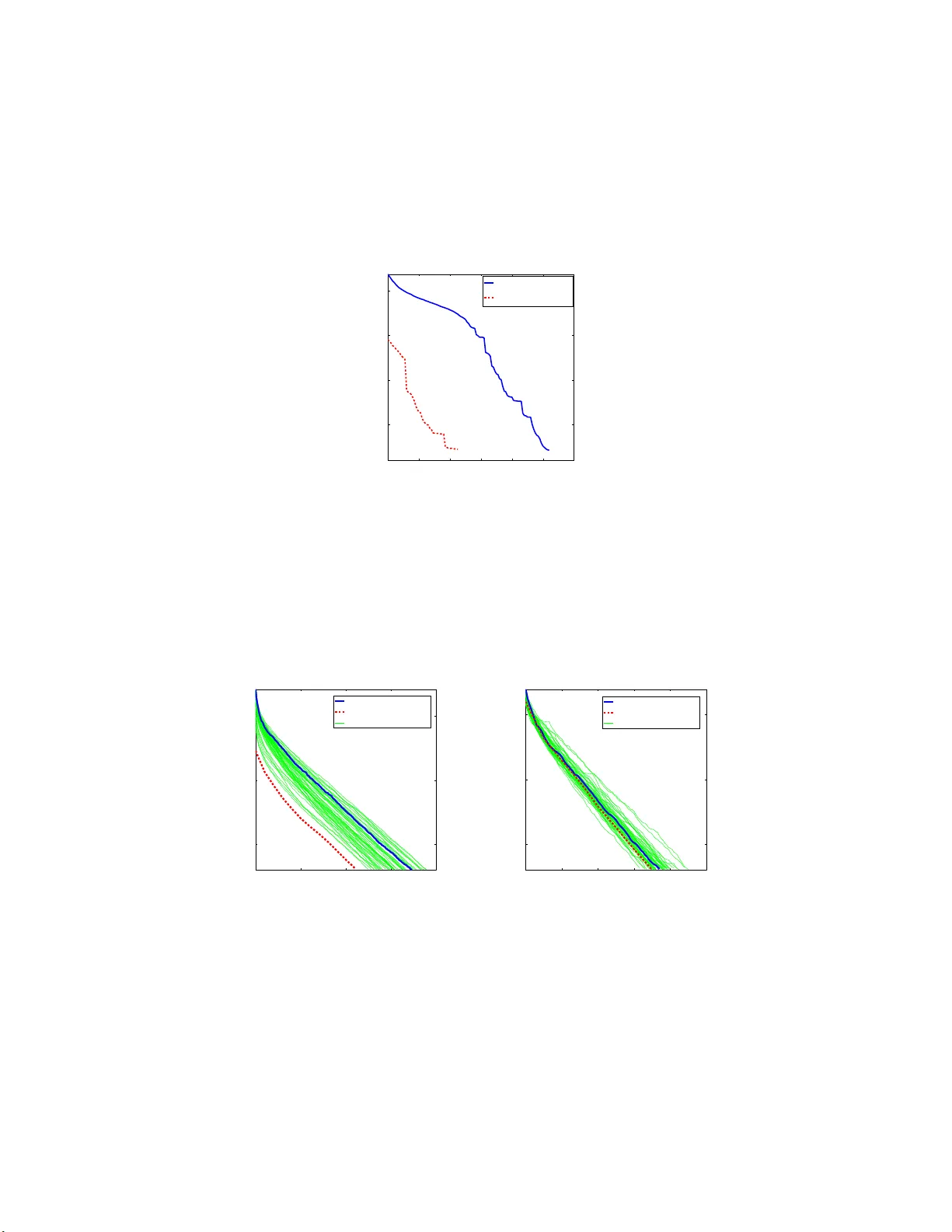
Iteration Compl exit y of Randomized Blo c k-Co ordinate Descen t Metho ds for Minimizing a Comp osite F unction ∗ P eter Rich tárik † Martin T a k áč ‡ Scho ol of Mathematics University of Edinbur gh Unite d Kingdom April 2011 (revised on July 4th, 2011) Abstract In this pap er w e develop a randomized block-coo rdinate d escent method fo r minimizing the sum of a smooth and a simple nonsmoo th blo c k-separable co n vex function and prov e that it obtains an ǫ -a ccurate solution with probability at lea st 1 − ρ in a t most O ( n ǫ log 1 ρ ) iteratio ns, where n is the num b er of blo cks. F or s trongly conv e x functions the metho d conv erg es linearly . This extends recent results of Nesterov [Efficiency o f co ordina te descent methods on hu ge-scale optimization problems, CO RE Discussion Paper #2010 /2], which c over the smo oth case, to comp osite minimization, while at the same time improving the complexity by the factor of 4 and removing ǫ from the logarithmic ter m. More imp ortantly , in contrast with the aforementioned work in whic h the author achiev es the results by a pplying the metho d to a regula rized version of the o b jective function with an unknown scaling factor, we show that this is not neces s ary , th us achieving true iteration co mplexit y bo unds. In the smo oth case we also allow for arbitrar y probability vectors and non-Euclidean norms. Finally , we demonstra te num erically that the algorithm is able to solve huge-scale ℓ 1 -regular ized lea st squar es and suppo rt vector machine problems with a billion v aria bles. Keyw ord s: Blo c k co or dinate descent, iteration complexity , comp osite minimization, co or- dinate rela xation, alternating minimization, conv ex optimization, L1-reg ularization, larg e s c a le suppo rt vector machines. 1 In tro duction The goal of this pap er, in the broadest sense, is to develo p efficien t metho ds for solving structured con vex optimization problems with some or all of these (not necess arily distinct) prop erties: ∗ The work of the first auth or w as supp orted in part by EPSRC grant EP/I01712 7/1 “Mathematics for v ast digital resources”. The second author was supported in part by the Cen tre for Nu merical Algorithms and Intelligen t Softw are (funded by EPSR C grant EP/G036 136/1 and th e Scottish F un ding Council). † School of Mathematics, Universit y of Edinburgh, UK, email: p eter.ric htarik@ed.ac.uk ‡ School of Mathematics, Universit y of Edinburgh, UK, email: m.tak ac@sms.ed.ac.uk 1 1. Size of Data. The s ize of the problem, measured as the dimension of the v ariable of in terest, is so large that the computation of a single function v alue or gradien t is prohibitiv e. There are severa l situations in whic h this is the case, let us mention t w o of them. • Memory . If the dimension of the space of v ariables is larger than the av ailable memory , the task of forming a gradien t or even of ev aluating the function v alue ma y b e imp ossible to execute and hence the usual gradien t metho ds will not w ork. • P atience. Even if the memory do es not preclude the p ossibilit y of taking a gradien t step, for large enough problems this step will take considerable time and, in some applications suc h as image pro cessing, users migh t prefer to see/ha v e some in termediary results b efore a single iteration is o v er. 2. Nature of Data. The nature and structure of data describing the problem ma y b e an obstacle in using curren t metho ds for v arious reasons, including the follo wing. • Completeness. If the data describing the problem is not immediately a v ailable in its en tiret y , but instead arrives incomplet e in pieces and blocks o v er time, with eac h blo c k “corresp onding to” one v ariable, it ma y not b e realistic (for v arious reasons suc h as “memory” and “patience” describ ed ab o ve) to wait for the en tire data set to arriv e b efore the optimization pro cess is started. • Source. If the data is distributed on a net work not all no des of whic h are equally resp onsiv e or functioning, it ma y b e necessary to work with whatev er data is av ailable at a given time. It app ears that a v ery reasonable approac h to solving some problems c haracterized ab ov e is to use ( blo ck) c o or di n ate desc ent metho ds (CD). In the remainder of this section w e mix argumen ts in supp ort of this claim with a brief review of the relev an t literature and an outline of our con tributions. 1.1 Blo c k Coor dinate Descen t Metho ds The basic algorithmic strategy of CD metho ds is kno wn in the literature under v arious names suc h as alternati ng minimization, co ordinate relaxation, linear and non-linear Gauss-Seidel metho ds, subspace correction and domain decomp osition. As w orking with all the v ariables of an optimization problem at eac h iteration ma y b e incon v enien t, difficult or imp ossible for any or all of the reasons men tioned ab o v e, the v ariables are partitioned into manageable blo cks, with eac h iteration fo cused on up dating a single block only , the remaining blo c k s b eing fix ed. Both for their conceptual and algorithmic simplicit y , CD metho ds w ere among the first optimization approac hes prop osed and studied in the literature (see [1] and the references therein; for a survey of block CD metho ds in semidefinite programmi ng we refer the reader to [24]). While they seem to ha ve nev er b elonged to the mainstream fo cus of the optimizatio n comm unit y , a renewed in terest in CD metho ds w as spark ed recen tly b y their successful application in sev eral areas—training supp ort vecto r mac hines in mac hine learning [5, 3, 17, 28, 29], optimizatio n [9 , 23, 21, 20, 31, 16, 13, 25 ], compressed sensing [8], regression [27], protein lo op closure [2] and truss top ology design [15]—partly due to a c hange in the size and natur e of data describ ed ab o v e. 2 Order of co or dinates. Efficiency of a CD metho d will necessarily dep end on the balance b et w een time sp ent on c ho osing the block to b e up dated in the curren t iteration and the qualit y of this c hoice in terms of f unction v alue decrease. One extreme p ossibility is a gr e e dy strategy in whic h the blo c k with the largest descen t or guaran teed descen t is chosen. In our setup s uc h a strategy is prohibitiv e as i) it wou ld require all data to b e a v ailable and ii) the w ork in v olv ed would b e excessive due to the size of the problem. Ev en if one is able to compute all partial deriv ativ es, it seems b etter to then take a full gradien t step instead of a co ordinate one, and a void thro wing almost all of the computed information a w ay . On the other end of the sp ectrum are t wo v ery c heap strategies for c ho osing the incum b en t co ordinate: cyclic and r andom . Surprisingly , it app ears that complexit y analysis of a cyclic CD metho d in s atisf ying generalit y has n ot yet b een done. The only attempt kno wn to us is the w ork of Saha and T ew ari [16 ]; the authors consider the case of minimizing a smo oth con vex function and pro ceed by establishing a sequence of comparison theorems b et w een the iterates of their method and the iterates of a s imple gradien t metho d. Their result requires an isotonicit y assumption. Note that a cyclic strategy assumes that the data describing the next blo c k is a v ailable when needed whic h ma y not alw ays b e realistic. The situation with a random strategy seems b etter; here are some of the reasons: (i) Recen t efforts suggest that complexit y results are p erhaps more readily obtained for random- ized metho ds and that randomization can actually improv e the con vergence rate [18, 6, 17]. (ii) Choos ing all blo c ks with equal probabilities s hould, i n tuitiv ely , lead to similar results as is the case with a cyclic strategy . In fact, a randomized strategy is able to a void wor st-case order of co ordinates, and hence migh t b e preferable. (iii) Randomized c hoice seems more suitable in cases when no t all data is a v ailable at all times. (iv) One ma y study the p ossibilit y of c ho osing blo c ks with different probabilities (w e do this in Section 4). The goal of suc h a strategy ma y b e either to impro ve the sp eed of the metho d (in Section 6.1 we intr o duce a sp eedup heuristic based on adaptiv ely c hanging the probabilities), or a more realistic mo deling of the av ailabilit y frequencies of the data defining eac h blo c k. Step size. Once a co ordinate (or a block of co ordinate s) is chosen to b e up dated in the curren t iteration, partial deriv ativ e can b e used to drive the steplength in the same wa y as it is done in the usual gradien t metho ds. As it is sometimes the case that the computation of a partial deriv ative is much che ap er and less memory demandi n g than the computation of the en tire gradien t, CD metho ds seem to b e promising candidates for problems describ ed ab o ve. It is imp ortan t that line searc h, if an y is implemen ted, is very efficien t. The en tire data set is either h uge or not av ailable and hence it is not reasonable to use function v alues at an y p oin t in the algorithm, including the line searc h. Instead, c heap partial deriv ative and other information derived f rom the problem structure should b e used to drive suc h a metho d. 1.2 Problem Description and Our Con tribution The pr oblem. In this pap er w e study the iter ation c omplexity of simple randomized blo c k co or- dinate decen t metho ds applied to the problem of minimizing a c omp osite obje ctive function , i.e., a function formed as the sum of a s mo oth con vex and a simple nonsmo oth con vex term: min x ∈ R N F ( x ) def = f ( x ) + Ψ( x ) . (1) 3 W e assume that this problem has a minim um ( F ∗ > −∞ ), f has (block) co ordinate Lipsc hitz gradien t, and Ψ is a (blo c k) separable prop er closed con vex extended real v alued function (these prop erties will b e defined precisely in Section 2). P ossible c hoices of Ψ include: (i) Ψ ≡ 0 . This co vers the case of smo oth minimi z ation . Complexit y results are given in [13]. (ii) Ψ is the indicator function of a blo ck-separ able conv ex s et (suc h as a b o x ). This c hoice mo dels pr oblems with c onstr aints on blo cks of variables ; iteration complexit y results are given in [13]. (iii) Ψ( x ) ≡ λ k x k 1 for λ > 0 . In this case w e can decomp os e R N on to N blo c ks. Increasing λ encourages the solution of (1) to b e sparser [26]. Applications ab ound in, for instance, mac hine learning [3], statistics [19] and signal process ing [8]. (iv) There are many more c hoices s uch as the elastic net [32], group lasso [30, 10 , 14] and sparse group lasso [4]. Iteration comp l exit y results. Strohmer and V ersh ynin [18] ha v e recen tly prop osed a random- ized Karczmarz method for solving o v erdetermined consisten t s ystems of linear equations and pro ved that the metho d enjoys global linear conv ergence whose rate can b e expressed in terms of the condi- tion n um b er of the underlying matrix. The authors claim that for certain problems their approac h can b e more efficien t than the conjugate gradien t method. Motiv ated b y these results, Lev en thal and Lewis [6] studied the problem of s olving a s y stem of linear eq uations and inequalities and in the pro cess ga ve iteration complexit y b ounds for a randomized CD metho d applied to the problem of minimizing a conv ex quadratic function. In their method the probabilit y of c hoice of eac h co ordinate is prop ortional to the corresp onding diagonal elemen t of the underlying p ositiv e s emidefin ite matrix defining the ob jectiv e function. These diagonal elemen ts can b e in terpreted as Lipschit z constan ts of the deriv ative of a restriction of the quadratic ob jectiv e onto one-dimensional lines parallel to the co ordinate axes. In the general (as opposed to quadratic) case considered in this pap er (1), these Lipsc hitz constan ts will play an imp ortan t role as w ell. Lin et al. [3] derived iteration complex- it y results f or severa l s mooth ob jective functions app earing in mac hine learning. Shalev-Sc h w arz and T ew ari [17] prop osed a randomize d co ordinate descen t metho d with uniform probabilities for minimizing ℓ 1 -regularized smo oth con v ex problems. They first transform the problem into a b o x constrained smo oth problem b y doubling the dimension and then apply a co ordinat e gradien t de- scen t metho d in whic h eac h co ordinate is chosen with eq ual probabilit y . Nestero v [13] has recent ly analyzed randomized co ordinate descen t metho ds in the smo oth unconstrained and b o x-constrained setting, in effect extending and impro ving up on some of the results in [6, 3, 17] in seve ral w ays. While the asymptotic c onver genc e r ates of some v arian ts of CD metho ds are w ell understoo d [9, 23, 21, 20 , 31], iter ati on c omplexity results are very rare. T o the b est of our know ledge, ran- domized CD algorithms for minimizing a comp osite f unction h a ve b een prop osed and analyzed (in the iteration complexit y sense) in a few sp ecial cases only: a) the unconstrained con vex quadratic case [6], b) the smo oth unconstrained ( Ψ ≡ 0 ) and the smo oth blo ck-co nstrained case ( Ψ is the indicator function of a direct sum of b o xes) [13] and c) the ℓ 1 -regularized case [17]. As the approac h in [17] is to rewrite the problem in to a s mo oth b o x-constrained format first, the results of [13] can b e view ed as a (ma jor) generalization and impro vemen t of those in [17] (the results wer e obtained independent ly). 4 Con tribution. In this pap er we further impro ve up on and extend and simplify the iteration complexit y results of Nestero v [13], treating the problem of minimizing the sum of a smo oth con vex and a simple nonsmo oth con v ex blo c k separable function (1). W e fo cus exclusiv ely on simple (as opposed to accelerated) metho ds. The reason for this is that the p er-iteration wo rk of the accelerated algorithm in [13] on h uge scale instances of problems with sp arse data (suc h as the Go ogle problem where sparsit y corresp onds to eac h w ebsite linking only to a few other w ebsites or the sparse problems w e consider in Section 6) is excessive. In fact, ev en the author do es not recommend using the accelerated metho d for solving suc h problems; the simple metho ds seem to b e more efficien t. Eac h algorithm of this pap er is supp orted b y a high probabilit y iteration complexit y result. That is, for an y giv en c onfidenc e level 0 < ρ < 1 and err or toler anc e ǫ > 0 , w e giv e an ex plicit expression for the n umber of iterations k whic h guaran tee that the metho d pro duces a random iterate x k for whic h P ( F ( x k ) − F ∗ ≤ ǫ ) ≥ 1 − ρ. T able 1 summarizes the main complexit y results of this paper . Algorithm 2—Uniform (blo c k) Co ordinate Descen t for Comp osite functions (UCDC)—is a metho d where at eac h iteration the blo c k of co ordinates to b e up dated (out of a total of n ≤ N blo c ks ) is c hosen uniformly at random. Algorithm 3—Randomized (blo c k) Co ordinate Descent for Smo oth functions (RC DS)—is a metho d where at eac h iteration blo c k i ∈ { 1 , . . . , n } is chosen with probabilit y p i . Both of these metho ds are sp ecial cases of the generic Algorithm 1; Randomized (blo c k) Co ordinate Descen t for Comp osite functions (RCDC ). Algorithm Ob jective Complexit y Algorithm 2 (U CDC) (Theorem 4) con vex composite 2 n max {R 2 L ( x 0 ) ,F ( x 0 ) − F ∗ } ǫ (1 + log 1 ρ ) 2 n R 2 L ( x 0 ) ǫ log  F ( x 0 ) − F ∗ ǫρ  Algorithm 2 (U CDC) (Theorem 7) strongly conv ex composite max { 4 µ , µ µ − 1 } n log  F ( x 0 ) − F ∗ ρǫ  Algorithm 3 (RCDS) (Theorem 11) con vex smooth 2 R 2 LP − 1 ( x 0 ) ǫ (1 + log 1 ρ ) − 2 Algorithm 3 (RCDS) (Theorem 12) strongly conv ex smooth 1 µ log  f ( x 0 ) − f ∗ ǫρ  T able 1: Summary of complexit y results obtained in this pape r. The sym b ols P , L, R 2 W ( x 0 ) and µ app earing in T able 1 will b e defined precisely in further sections. F or no w it suffices to sa y that L enco des the (blo c k) co ordinate Lipsc hitz constan ts of the gradien t of f , P enco des the probabilities { p i } , R 2 W ( x 0 ) is a measure of distance of the initial iterate x 0 from the set of minimizers of the problem (1 ) in a norm defined by W (see Section 2) and µ is the strong con v exit y parameter of F (see Section 3.2). In the nonsmooth case µ dep ends on L and the smo oth case it dep ends b oth on L and P . Let us no w briefly outline the main similarities and differences b etw een our results and those in [13]. A more detailed and expanded discussion can b e found in Section 5. 5 1. Comp osite setting. W e consider the comp osite setting (1), whereas [13] co vers the uncon- strained and constrained smo oth setting only . 2. No n eed for regularization. Nestero v’s high probabilit y results in the case of minimizing a function whic h is not s trongly con vex are based on regularizing the ob j ectiv e to mak e it strongly con vex and then running the metho d on the regularized function. Our contrib ution here is that we show that no regularization is needed b y doing a more detailed analysis using a thresholding argumen t (Theorem 1 ). 3. Better com plexit y . Our complexit y results are b etter by the constant f actor of 4. Also, w e ha ve remo v ed ǫ f rom under the logarithm. 4. General probabili ties. Nestero v considers probabilities p i prop ortiona l to L α i , where α ≥ 0 is a parameter. High probabilit y results are pro ved in [13] f or α ∈ { 0 , 1 } only . Our results in the smo oth case hold for an arbitrary probabilit y v ector p . 5. General norm s. Nes tero v’s exp ectation results (Theorems 1 and 2) are prov ed for general norms. How ev er, his high probabilit y results are pro ved for Euclidean norms only . In our approac h all results hold for general norms. 6. Simplification. Our analysis is more compact. In the num erical exp erimen ts s ection w e fo cus on sp arse ℓ 1 -regularized regression and supp ort v ector mac hine problems. F or these problems w e in tro duce a p o werful sp e e dup heuristic based on adaptiv ely chang ing the probabilit y v ector throughout the iterations (Section 6.1; “sp eedup b y shrinking”). Con ten ts. This pap er is organized as follo ws. W e start in Section 2 b y defining basic notation, describing the blo c k s tructur e of the problem, stating assumptions and describing the generic ran- domized blo c k-co ordinate descen t algorithm (R CDC). In Section 3 we study the p erformance of a uniform v arian t (UCDC) of RCDC as applied to a composite ob jective f unction and in Section 4 w e analyze a smo oth v arian t (RCDS ) of RCDC; that is, w e study t he p erformance of R CDC on a s mo oth ob jectiv e f unction. In Section 5 w e compare kno wn complexit y results for CD methods with the ones established in this pap er. Finally , in Section 6 w e demonstrate the efficiency of the method on ℓ 1 -regularized sparse regression and linear supp ort v ector mach ine problems. 2 Assumptions and the Algorithm Blo c k structure. W e mo del the block structure of the problem by decomp osing the space R N in to n subspaces as follo ws. Let U ∈ R N × N b e a column p erm utation of the N × N ident it y matrix and further let U = [ U 1 , U 2 , . . . , U n ] b e a decomp osition of U in to n submatrices, with U i b eing of size N × N i , where P i N i = N . Clearly , an y v ector x ∈ R N can b e written uniquely as x = P i U i x ( i ) , where x ( i ) = U T i x ∈ R i ≡ R N i . Also note that U T i U j = ( N i × N i iden tit y matrix, if i = j, N i × N j zero matrix, otherwise. (2) 6 F or simplicit y w e will write x = ( x (1) , . . . , x ( n ) ) T . W e equip R i with a pair of conjugate Euclidean norms: k t k ( i ) = h B i t, t i 1 / 2 , k t k ∗ ( i ) = h B − 1 i t, t i 1 / 2 , t ∈ R i , (3) where B i ∈ R N i × N i is a p ositiv e definite matrix and h· , ·i is the standard Euclidean inner pro duct. Example 1. L et n = N , N i = 1 for al l i and U = [ e 1 , e 2 , . . . , e n ] b e the n × n identity matrix. Then U i = e i is the i -th uni t ve ctor and x ( i ) = e T i x ∈ R i = R is the i -th c o or dinate of x . Also, x = P i e i x ( i ) . If we let B i = 1 for al l i , then k t k ( i ) = k t k ∗ ( i ) = | t | for al l t ∈ R . Smo othness of f . W e as sume throughout the pap er that the gradien t of f is blo c k co ordinate- wise Lipsc hitz, uniformly in x , with p ositiv e constant s L 1 , . . . , L n , i.e., that for all x ∈ R N , t ∈ R i and i we hav e k∇ i f ( x + U i t ) − ∇ i f ( x ) k ∗ ( i ) ≤ L i k t k ( i ) , (4) where ∇ i f ( x ) def = ( ∇ f ( x )) ( i ) = U T i ∇ f ( x ) ∈ R i . (5) An imp ortan t consequence of (4) is the f ollo wing standard inequalit y [11]: f ( x + U i t ) ≤ f ( x ) + h∇ i f ( x ) , t i + L i 2 k t k 2 ( i ) . (6) Separabilit y of Ψ . W e assume that Ψ is blo c k separable, i.e., that it can b e decomposed as follo ws: Ψ( x ) = n X i =1 Ψ i ( x ( i ) ) , (7) where the functions Ψ i : R i → R are conv ex and closed. The algorithm. Notice that an upper b ound on F ( x + U i t ) , view ed as a f unction of t ∈ R i , is readily a v ailable: F ( x + U i t ) (1) = f ( x + U i t ) + Ψ( x + U i t ) (6) ≤ f ( x ) + V i ( x, t ) + C i ( x ) , (8) where V i ( x, t ) def = h∇ i f ( x ) , t i + L i 2 k t k 2 ( i ) + Ψ i ( x ( i ) + t ) (9) and C i ( x ) def = X j 6 = i Ψ j ( x ( j ) ) . (10) W e are no w ready to describ e the generic metho d. Giv en iterate x k , Algorithm 1 picks blo ck i k = i ∈ { 1 , 2 , . . . , n } with probabilit y p i > 0 and then up dates the i -th blo c k of x k so as to minimize (exactly) in t the upp er b ound (8) on F ( x k + U i t ) . Note that in certain cases it is p ossible to minimize F ( x k + U i t ) directly; p erhaps in a closed form. This is the case, f or example, when f is a con v ex q uadratic. The iterates { x k } are random vect ors and the v alues { F ( x k ) } are random v ariables. Clearly , x k +1 dep ends only on x k . As our analysis will b e based on the (exp ected) p er-iteration decrease of the ob jectiv e function, the results will hold even if w e replace V i ( x k , t ) b y F ( x k + U i t ) in Algorithm 1. 7 Algorithm 1 RC DC ( p, x 0 ) ( R andomized C o ordinate D escen t for C omp osite F unctions) for k = 0 , 1 , 2 , . . . do Cho ose i k = i ∈ { 1 , 2 , . . . , n } with probabilit y p i T ( i ) ( x k ) def = arg min { V i ( x k , t ) : t ∈ R i } x k +1 = x k + U i T ( i ) ( x k ) end for Global structure. F or fixed p ositive s calars w 1 , . . . , w n let W = Diag( w 1 , . . . , w n ) and define a pair of conjugate norms in R N b y k x k W = " n X i =1 w i k x ( i ) k 2 ( i ) # 1 / 2 , (11) k y k ∗ W = m ax k x k W ≤ 1 h y , x i = " n X i =1 w − 1 i ( k y ( i ) k ∗ ( i ) ) 2 # 1 / 2 . (12) In the the subsequen t analysis w e will use W = L (Section 3) and W = LP − 1 (Section 4), where L = Diag ( L 1 , . . . , L n ) and P = Diag( p 1 , . . . , p n ) . The set of optimal solutions of (1) is denoted by X ∗ and x ∗ is an y elemen t of that set. Define R W ( x ) = max y max x ∗ ∈ X ∗ {k y − x ∗ k W : F ( y ) ≤ F ( x ) } , whic h is a measure of the size of the level set of F giv en b y x . I n most of the results in this pap er w e will need to assume that R W ( x 0 ) is finite for the initial iterate x 0 and W = L or W = L P − 1 . A tec h nical result. The next s imple result is the main tec hnical to ol enabling us to s implify and impro ve the corresp onding analysis in [13]. It will b e used with ξ k = F ( x k ) − F ∗ . Theorem 1. L et ξ 0 > 0 b e a c onstant, 0 < ǫ < ξ 0 , and c onsi der a nonne gative n onincr e asing se quenc e of (discr ete) r andom variables { ξ k } k ≥ 0 with one of the fol lowing pr op erties: (i) E [ ξ k +1 | ξ k ] ≤ ξ k − ξ 2 k c , for al l k , wher e c > 0 is a c onstant, (ii) E [ ξ k +1 | ξ k ] ≤ (1 − 1 c ) ξ k , for al l k such that ξ k ≥ ǫ , wher e c > 1 is a c onstant. Cho ose c onfidenc e level ρ ∈ (0 , 1) . If pr op erty (i) holds and we cho ose ǫ < c and K ≥ c ǫ (1 + log 1 ρ ) + 2 − c ξ 0 , (13) or if pr op erty (ii ) holds, and we cho ose K ≥ c log ξ 0 ǫρ , (14) then P ( ξ K ≤ ǫ ) ≥ 1 − ρ. (15) 8 Pr o of. Notice that the sequence { ξ ǫ k } k ≥ 0 defined by ξ ǫ k = ( ξ k if ξ k ≥ ǫ, 0 otherwise, satisfies ξ ǫ k ≤ ǫ ⇔ ξ k ≤ ǫ, k ≥ 0 . (16) Therefore, b y Marko v inequalit y , P ( ξ k > ǫ ) = P ( ξ ǫ k > ǫ ) ≤ E [ ξ ǫ k ] ǫ , and hence it suffices to sho w that θ K ≤ ǫρ, (17) where θ k def = E [ ξ ǫ k ] . If prop ert y (i) holds, then E [ ξ ǫ k +1 | ξ ǫ k ] ≤ ξ ǫ k − ( ξ ǫ k ) 2 c , E [ ξ ǫ k +1 | ξ ǫ k ] ≤ (1 − ǫ c ) ξ ǫ k , k ≥ 0 , (18) and b y taking exp ectations (using con vexit y of t 7→ t 2 in the first case) w e obtain θ k +1 ≤ θ k − θ 2 k c , k ≥ 0 , (19) θ k +1 ≤ (1 − ǫ c ) θ k , k ≥ 0 . (20) Notice that (19) is b etter than (20) precisely when θ k > ǫ . Since 1 θ k +1 − 1 θ k = θ k − θ k +1 θ k +1 θ k ≥ θ k − θ k +1 θ 2 k (19) ≥ 1 c , w e hav e 1 θ k ≥ 1 θ 0 + k c = 1 ξ 0 + k c . Therefore, if w e let k 1 ≥ c ǫ − c ξ 0 , we obtain θ k 1 ≤ ǫ . Finally , letting k 2 ≥ c ǫ log 1 ρ , we hav e θ K (13) ≤ θ k 1 + k 2 (20) ≤ (1 − ǫ c ) k 2 θ k 1 ≤ ((1 − ǫ c ) 1 ǫ ) c log 1 ρ ǫ ≤ ( e − 1 c ) c log 1 ρ ǫ = ǫρ, establishing (17). I f prop ert y (ii) holds, then E [ ξ ǫ k +1 | ξ ǫ k ] ≤ (1 − 1 c ) ξ ǫ k for all k , and hence θ K ≤ (1 − 1 c ) K θ 0 = (1 − 1 c ) K ξ 0 (14) ≤ ((1 − 1 c ) c ) log ξ 0 ǫρ ξ 0 ≤ ( e − 1 ) log ξ 0 ǫρ ξ 0 = ǫρ, again establishing (17). Restarting. Note that similar, alb eit slightly we aker, high probabilit y results can b e ach iev ed b y r estarting as follo ws. W e run the random pro cess { ξ k } rep eatedly r = ⌈ log 1 ρ ⌉ times, alw ays starting from ξ 0 , eac h time f or the s ame n um b er of iterations k 1 for whic h P ( ξ k 1 > ǫ ) ≤ 1 e . It then f ollo ws that the probabilit y that all r v alues ξ k 1 will b e larger than ǫ is at most ( 1 e ) r ≤ ρ . Note that the restarting tec hnique demands that we p erform r ev aluations of the ob jectiv e function; this is not needed in the one-shot approac h co v ered b y the theorem. 9 It remains to estimate k 1 in the t w o cases of Theorem 1. W e argue that in case (i) w e can choose k 1 = ⌈ c ǫ/e − c ξ 0 ⌉ . I ndeed, using similar argumen ts as in Theorem 1 this leads to E [ ξ k 1 ] ≤ ǫ e , which b y Marko v inequalit y implies that in a single run of the pro cess we ha ve P ( ξ k 1 > ǫ ) ≤ E [ ξ k 1 ] ǫ ≤ ǫ/e ǫ = 1 e . Therefore, K = ⌈ ec ǫ − c ξ 0 ⌉⌈ log 1 ρ ⌉ iterations suffice in case (i). A similar restarting tec hnique can b e applied in case (ii). Tigh tness. It can b e sho wn on simple examples that the b ounds in the ab o v e result are tight . 3 Co ordinate Descen t for Comp osite F unctions In this s ection w e study the p erformance of Algorithm 1 in the sp ecial case when all probabilities are c hosen to b e the same, i.e., p i = 1 n for all i . F or easier future reference w e set this metho d apart and giv e it a name (Algorithm 2). Algorithm 2 UCDC ( x 0 ) ( U niform C o ordinate D escent f or C omp osite F unctions) for k = 0 , 1 , 2 , . . . do Cho ose i k = i ∈ { 1 , 2 , . . . , n } with probabilit y 1 n T ( i ) ( x k ) = arg min { V i ( x k , t ) : t ∈ R i } x k +1 = x k + U i T ( i ) ( x k ) end for The follo wing function plays a cen tral role in our analysis: H ( x, T ) def = f ( x ) + h∇ f ( x ) , T i + 1 2 k T k 2 L + Ψ( x + T ) . (21) Comparing (21) with (9) using (2), (5), (7) and (11) w e get H ( x, T ) = f ( x ) + n X i =1 V i ( x, T ( i ) ) . (22) Therefore, the vector T ( x ) = ( T (1) ( x ) , . . . , T ( n ) ( x )) , with the comp onen ts T ( i ) ( x ) defined in Algo- rithm 1, is the minimizer of H ( x, · ) : T ( x ) = arg min T ∈ R N H ( x, T ) . (23) Let us start b y establishing an auxiliary result whic h will b e used rep eatedly . Lemma 2. L et { x k } , k ≥ 0 , b e the r andom iter ates gener ate d by UC DC ( x 0 ) . Then E [ F ( x k +1 ) − F ∗ | x k ] ≤ 1 n ( H ( x k , T ( x k )) − F ∗ ) + n − 1 n ( F ( x k ) − F ∗ ) . (24) 10 Pr o of. E [ F ( x k +1 ) | x k ] = n X i =1 1 n F ( x k + U i T ( i ) ( x k )) (8) ≤ 1 n n X i =1 [ f ( x k ) + V i ( x k , T ( i ) ( x k )) + C i ( x k )] (22) = 1 n H ( x k , T ( x k )) + n − 1 n f ( x k ) + 1 n n X i =1 C i ( x k ) (10) = 1 n H ( x k , T ( x k )) + n − 1 n f ( x k ) + 1 n n X i =1 X j 6 = i Ψ j ( x ( j ) k ) = 1 n H ( x k , T ( x k )) + n − 1 n F ( x k ) . 3.1 Con vex Ob jective In order for Lemma 2 to b e useful, w e need to estimate H ( x k , T ( x k )) − F ∗ from ab o v e in terms of F ( x k ) − F ∗ . Lemma 3. Fix x ∗ ∈ X ∗ , x ∈ d om Ψ and let R = k x − x ∗ k L . Then H ( x, T ( x )) − F ∗ ≤ (  1 − F ( x ) − F ∗ 2 R 2  ( F ( x ) − F ∗ ) , if F ( x ) − F ∗ ≤ R 2 , 1 2 R 2 < 1 2 ( F ( x ) − F ∗ ) , otherwise. (25) Pr o of. H ( x, T ( x )) (23) = min T ∈ R N H ( x, T ) = min y ∈ R N H ( x, y − x ) (21) ≤ min y ∈ R N f ( x ) + h∇ f ( x ) , y − x i + Ψ( y ) + 1 2 k y − x k 2 L ≤ min y ∈ R N F ( y ) + 1 2 k y − x k 2 L ≤ m in α ∈ [0 , 1] F ( αx ∗ + (1 − α ) x ) + α 2 2 k x − x ∗ k 2 L ≤ m in α ∈ [0 , 1] F ( x ) − α ( F ( x ) − F ∗ ) + α 2 2 R 2 . (26) Minimizing (26) in α giv es α ∗ = min  1 , ( F ( x ) − F ∗ ) /R 2  ; the result follow s. W e are now ready to estimate the nu m b er of iterations needed to push the ob jective v alue within ǫ of the optimal v alue with high probabilit y . Note that s ince ρ app ears under the logarithm and hence it is easy to attain high confidence . Theorem 4. Cho ose in itial p oint x 0 and tar get c onfidenc e 0 < ρ < 1 . F urther, let the tar get ac cur acy ǫ > 0 and i ter ation c ounter k b e chosen i n an y of the fol lowing two ways: 11 (i) ǫ < F ( x 0 ) − F ∗ and k ≥ 2 n max {R 2 L ( x 0 ) ,F ( x 0 ) − F ∗ } ǫ  1 + log 1 ρ  + 2 − 2 n max {R 2 L ( x 0 ) ,F ( x 0 ) − F ∗ } F ( x 0 ) − F ∗ , (27) (ii) ǫ < min {R 2 L ( x 0 ) , F ( x 0 ) − F ∗ } and k ≥ 2 n R 2 L ( x 0 ) ǫ log F ( x 0 ) − F ∗ ǫρ . (28) If x k is the r andom p oi n t gener ate d by UC DC ( x 0 ) as applie d to the c onvex function F , then P ( F ( x k ) − F ∗ ≤ ǫ ) ≥ 1 − ρ. Pr o of. Since F ( x k ) ≤ F ( x 0 ) for all k , w e ha ve k x k − x ∗ k L ≤ R L ( x 0 ) for all x ∗ ∈ X ∗ . Lemma 2 together with Lemma 3 then imply that the follo wing holds for all k : E [ F ( x k +1 ) − F ∗ | x k ] ≤ 1 n max n 1 − F ( x k ) − F ∗ 2 k x k − x ∗ k 2 L , 1 2 o ( F ( x k ) − F ∗ ) + n − 1 n ( F ( x k ) − F ∗ ) = max n 1 − F ( x k ) − F ∗ 2 n k x k − x ∗ k 2 L , 1 − 1 2 n o ( F ( x k ) − F ∗ ) ≤ max n 1 − F ( x k ) − F ∗ 2 n R 2 L ( x 0 ) , 1 − 1 2 n o ( F ( x k ) − F ∗ ) . (29) Let ξ k = F ( x k ) − F ∗ and consider case (i). If we let c = 2 n max {R 2 L ( x 0 ) , F ( x 0 ) − F ∗ } , then from (29) w e obtain E [ ξ k +1 | ξ k ] ≤ (1 − ξ k c ) ξ k = ξ k − ξ 2 k c , k ≥ 0 . Moreo ver, ǫ < ξ 0 < c . The result then follo ws b y applying Theorem 1. Consider no w case (ii). Letting c = 2 n R 2 L ( x 0 ) ǫ > 1 , notice that if ξ k ≥ ǫ , inequalit y (29) implies that E [ ξ k +1 | ξ k ] ≤ m ax n 1 − ǫ 2 n R 2 L ( x 0 ) , 1 − 1 2 n o ξ k = (1 − 1 c ) ξ k . Again, the result f ollo ws f rom Theorem 1. 3.2 Strongly Con v ex Ob jectiv e Assume that F is strongly con vex with resp ect to some norm k · k with con vexit y parameter µ > 0 ; that is, F ( x ) ≥ F ( y ) + h F ′ ( y ) , x − y i + µ 2 k x − y k 2 , x, y ∈ dom F , (30) where F ′ ( y ) is an y subgradien t of F at y . Note that from the first order optimalit y conditions for (1) w e obtain h F ′ ( x ∗ ) , x − x ∗ i ≥ 0 f or all x ∈ dom F whic h, com bining with (30) used with y = x ∗ , yields the standard inequality F ( x ) − F ∗ ≥ µ 2 k x − x ∗ k 2 , x ∈ dom F . (31) The next lemma will b e us ef ul in pro ving linear con v ergence of the exp ected v alue of the ob jectiv e function to the minim um. 12 Lemma 5. If F is str ongly c onvex wi th r esp e ct to k · k L with c on vex ity p ar ameter µ > 0 , then H ( x, T ( x )) − F ∗ ≤ γ µ ( F ( x ) − F ∗ ) , x ∈ dom F , (32) wher e γ µ = ( 1 − µ 4 , if µ ≤ 2 , 1 µ , otherwise. (33) Pr o of. H ( x, T ( x )) (23) = min t ∈ R N H ( x, t ) = min y ∈ R N H ( x, y − x ) ≤ min y ∈ R N F ( y ) + 1 2 k y − x k 2 L ≤ min α ∈ [0 , 1] F ( αx ∗ + (1 − α ) x ) + α 2 2 k x − x ∗ k 2 L ≤ min α ∈ [0 , 1] F ( x ) − α ( F ( x ) − F ∗ ) + α 2 2 k x − x ∗ k 2 L (31) ≤ min α ∈ [0 , 1] F ( x ) + α  α µ − 1  ( F ( x ) − F ∗ ) . (34) The optimal α in (34) is α ∗ = min  1 , µ 2  ; the result follo ws. W e no w sho w that the exp ected v alue of F ( x k ) con verges to F ∗ linearly . Theorem 6. L et F b e str ongly c onvex with r esp e ct to the norm k · k L with c onvexity p ar ameter µ > 0 . If x k is the r andom p oint gener ate d UCDC ( x 0 ) , then E [ F ( x k ) − F ∗ ] ≤  1 − 1 − γ µ n  k ( F ( x 0 ) − F ∗ ) , (35) wher e γ µ is define d by (33). Pr o of. F ollo ws from Lemma 2 and Lemma 5. The follo wing is an analogue of Theorem 4 in the case of a strongly conv ex ob jective. Note that b oth the accuracy and confidence parameters app ear under the logarithm. Theorem 7. L et F b e str ongly c onvex with r esp e ct to k · k L with c onvexity p ar ameter µ > 0 and cho ose ac cur acy level ǫ > 0 , c onfidenc e level 0 < ρ < 1 , and k ≥ n 1 − γ µ log  F ( x 0 ) − F ∗ ρǫ  , (36) wher e γ µ is given by (33) . I f x k is the r andom p oi n t gener ate d by UC DC ( x 0 ) , then P ( F ( x k ) − F ∗ ≤ ǫ ) ≥ 1 − ρ. Pr o of. Using Marko v inequalit y and Theorem 6, w e obtain P [ F ( x k ) − F ∗ ≥ ǫ ] ≤ 1 ǫ E [ F ( x k ) − F ∗ ] (35) ≤ 1 ǫ  1 − 1 − γ µ n  k ( F ( x 0 ) − F ∗ ) (36) ≤ ρ. 13 3.3 A Regularization T echni que In this part we will in v es tigate an alternativ e approac h to establishing an iteration complexit y result in the case of an ob j ectiv e function that is not strongly con v ex. The strategy is v ery simple. W e first regularize the ob jective function b y adding a small quadratic term to it, th us making it strongly con vex, and then argue that when Algorithm 2 is applied to the regulari zed ob jective , we can reco ver an appro x imate solution of the original non-regularized problem. The result obtained in this w a y is sligh tly differen t to the one co vered by Theorem 4 in that 2 n R 2 L ( x 0 ) is replaced b y 4 n k x 0 − x ∗ k 2 L . In some situations, k x 0 − x ∗ k 2 L can b e significan tly smaller than R 2 L ( x 0 ) . H ow ev er, let us remark that the regularizing term dep ends on quantiti es that are not known in adv ance. Fix x 0 and ǫ > 0 and consider a regularized v ersion of the ob jective f unction defined b y F µ ( x ) def = F ( x ) + µ 2 k x − x 0 k 2 L , µ = ǫ k x 0 − x ∗ k 2 L . (37) Clearly , F µ is strongly con vex with resp ect to the norm k · k L with con vexit y parameter µ . In the rest of this subsection w e sho w that if w e apply UCDC ( x 0 ) to F µ with target accuracy ǫ 2 , then with high probabilit y we reco v er an ǫ -appro ximate s olution of (1). W e first need to establish that an appro ximate minimizer of F µ m ust b e an appro ximate minimizer of F . Lemma 8. If x ′ satisfies F µ ( x ′ ) ≤ m in x ∈ R N F µ ( x ) + ǫ 2 , then F ( x ′ ) ≤ F ∗ + ǫ . Pr o of. Clearly , F ( x ) ≤ F µ ( x ) , x ∈ R N . (38) If w e let x ∗ µ def = arg m in x ∈ R N F µ ( x ) , then by assumption, F µ ( x ′ ) − F µ ( x ∗ µ ) ≤ ǫ 2 , (39) and F µ ( x ∗ µ ) = min x ∈ R N F ( x ) + µ 2 k x − x 0 k 2 L ≤ F ( x ∗ ) + µ 2 k x ∗ − x 0 k 2 L (37) ≤ F ( x ∗ ) + ǫ 2 . (40) Putting all these observ ations together, w e get 0 ≤ F ( x ′ ) − F ( x ∗ ) (38) ≤ F µ ( x ′ ) − F ( x ∗ ) (39) ≤ F µ ( x ∗ µ ) + ǫ 2 − F ( x ∗ ) (40) ≤ ǫ. The follo wing theorem is an analogue of Theorem 4. Theorem 9. Cho ose initial p oin t x 0 , tar get ac cur acy 0 < ǫ ≤ 2 k x 0 − x ∗ k 2 L , (41) tar get c onfi denc e level 0 < ρ < 1 , and k ≥ 4 n k x 0 − x ∗ k 2 L ǫ log  2( F ( x 0 ) − F ∗ ) ρǫ  . (42) If x k is the r andom p oi n t gener ate d by UC DC ( x 0 ) as applie d to F µ , then P ( F ( x k ) − F ∗ ≤ ǫ ) ≥ 1 − ρ. 14 Pr o of. Let us apply Theorem 7 to the problem of minimizing F µ , comp osed as f + Ψ µ , with Ψ µ ( x ) = Ψ( x ) + µ 2 k x − x 0 k 2 L . Note that F µ ( x 0 ) − F µ ( x ∗ µ ) (37) = F ( x 0 ) − F µ ( x ∗ µ ) (38) ≤ F ( x 0 ) − F ( x ∗ µ ) ≤ F ( x 0 ) − F ∗ , (43) and n 1 − γ µ (33) , (37) , (41) = 4 n k x 0 − x ∗ k 2 L ǫ . (44) Comparing (36) and (42) in view of (43) and (44), Theorem 7 implies that P ( F µ ( x k ) − F µ ( x ∗ µ ) ≤ ǫ 2 ) ≥ 1 − ρ. It no w suffices to apply Lemma 8. 4 Co ordinate Descen t for Smo oth F unctions In this s ection w e give a m uc h simplified and impro v ed treatmen t of the smo oth case ( Ψ ≡ 0 ) as compared to the analysis in Sections 2 and 3 of [13]. As alluded to in the ab o v e, w e will dev elop the analysis in the smo oth case for arbitrary , p ossibly non-Euclid ean, norms k · k ( i ) , i = 1 , 2 , . . . , n . Let k · k b e an arbitrary norm in R l . Then its dual is defined in the usual w ay: k s k ∗ = max k t k =1 h s, t i . The f ollowin g (Lemma 10) is a simple result whic h is used in [1 3] without b eing fully articulated nor pro ved as it constitutes a straigh tforw ard extension of a fact that is trivial in the Euclidean setting to the case of general norms. Since w e think it is p erhaps not standard, we b eliev e it deserves to b e sp elled out explicitly . The lemma has the follow ing use . The main problem whic h needs to b e solv ed at each iteration of Algorithm 1 in the smo oth case is of the form (45), with s = − 1 L i ∇ i f ( x k ) and k · k = k · k ( i ) . Since k · k is non-Euclidean, we cannot write dow n the solution of (45) in a closed form a-priori, for all norms. Neverthel ess, w e can sa y something ab out the solution, whic h turns out to b e enough for our subsequent analysis . Lemma 10. If by s # we denote an optimal solution of the pr oblem min t n u ( s ) def = −h s, t i + 1 2 k t k 2 o , (45) then u ( s # ) = − 1 2 ( k s k ∗ ) 2 , k s # k = k s k ∗ , ( αs ) # = α ( s # ) , α ∈ R . (46) Pr o of. F or α = 0 the last s tatemen t is trivial. If w e fix α 6 = 0 , then clearly u (( αs ) # ) = min k t k =1 min β {−h αs, β t i + 1 2 k β t k 2 } . F or fixed t the solution of the inner problem is β = h αs, t i , whence u (( αs ) # ) = min k t k =1 − 1 2 h αs, t i 2 = − 1 2 α 2  max k t k =1 h s, t i  2 = − 1 2 ( k αs k ∗ ) 2 , (47) 15 pro ving the first claim. Next, note that optimal t = t ∗ in (47) maximizes h s, t i ov er k t k = 1 and hence h s, t ∗ i = k s k ∗ , whic h implies that k ( αs ) # k = | β ∗ | = |h αs, t ∗ i| = | α ||h s, t ∗ i| = | α |k s k ∗ = k αs k ∗ , giving the second claim. Finally , since t ∗ dep ends on s only , w e ha ve ( αs ) # = β ∗ t ∗ = h αs, t ∗ i t ∗ and, in particular, s # = h s, t ∗ i t ∗ . Therefore, ( αs ) # = α ( s # ) . W e can use Lemma 10 to rewrite the main step of Algorithm 1 in the smo oth case in to the more explicit form, T ( i ) ( x ) = arg min t ∈ R i V i ( x, t ) (9) = arg min t ∈ R i h∇ i f ( x ) , t i + L i 2 k t k 2 ( i ) (45) =  − ∇ i f ( x ) L i  # (46) = − 1 L i ( ∇ i f ( x )) # , leading to Algorithm 3. Algorithm 3 RC DS ( p, x 0 ) ( R andomized C o ordinate D escen t f or S mo oth F unction s) for k = 0 , 1 , 2 , . . . do Cho ose i k = i ∈ { 1 , 2 , . . . , n } with probabilit y p i x k +1 = x k − 1 L i U i ( ∇ i f ( x k )) # end for The main utilit y of Lemma 10 for the purp ose of the subsequen t complexit y analysis comes from the f act that it enables us to giv e an explicit b ound on the decrease in the ob jective function during one iteration of the method in the s ame form as in the Euclidean case: f ( x ) − f ( x + U i T ( i ) ( x )) (6) ≥ − [ h∇ i f ( x ) , T ( i ) ( x ) i + L i 2 k T ( i ) ( x ) k 2 ( i ) ] = − L i u (( − ∇ i f ( x ) L i ) # ) (48) (46) = L i 2 ( k − ∇ i f ( x ) L i k ∗ ( i ) ) 2 = 1 2 L i ( k∇ i f ( x ) k ∗ ( i ) ) 2 . 4.1 Con vex Ob jective W e are no w ready to state the main result of this section. Theorem 11. Cho ose ini tial p oin t x 0 , tar get ac cur acy 0 < ǫ < min { f ( x 0 ) − f ∗ , 2 R 2 LP − 1 ( x 0 ) } , tar get c onfi denc e 0 < ρ < 1 and k ≥ 2 R 2 LP − 1 ( x 0 ) ǫ  1 + log 1 ρ  + 2 − 2 R 2 LP − 1 ( x 0 ) f ( x 0 ) − f ∗ , (49) or k ≥ 2 R 2 LP − 1 ( x 0 ) ǫ  1 + log 1 ρ  − 2 . (50) If x k is the r andom p oi n t gener ate d by RCDS ( p, x 0 ) as applie d to c onvex f , then P ( f ( x k ) − f ∗ ≤ ǫ ) ≥ 1 − ρ. 16 Pr o of. Let us first estimate the exp ected decrease of the ob jectiv e function during one iteration of the metho d: f ( x k ) − E [ f ( x k +1 ) | x k ] = n X i =1 p i [ f ( x k ) − f ( x k + U i T ( i ) ( x k ))] (48) ≥ 1 2 n X i =1 p i 1 L i ( k∇ i f ( x k ) k ∗ ( i ) ) 2 = 1 2 ( k∇ f ( x k ) k ∗ W ) 2 , where W = LP − 1 . Since f ( x k ) ≤ f ( x 0 ) for all k and b ecause f is con vex, w e get f ( x k ) − f ∗ ≤ max x ∗ ∈ X ∗ h∇ f ( x k ) , x k − x ∗ i ≤ k∇ f ( x k ) k ∗ W R W ( x 0 ) , whence f ( x k ) − E [ f ( x k +1 ) | x k ] ≥ 1 2  f ( x k ) − f ∗ R W ( x 0 )  2 . By rearranging the terms w e obtain E [ f ( x k +1 ) − f ∗ | x k ] ≤ f ( x k ) − f ∗ − ( f ( x k ) − f ∗ ) 2 2 R 2 W ( x 0 ) . If we now use Theorem 1 with ξ k = f ( x k ) − f ∗ and c = 2 R 2 W ( x 0 ) , w e obtain the result for k given b y (49). W e no w claim that 2 − c ξ 0 ≤ − 2 , from whic h it follo ws that the result holds for k given b y (50). Indeed, first notice that this inequalit y is eq uiv alent to f ( x 0 ) − f ∗ ≤ 1 2 R 2 W ( x 0 ) . (51) No w, a straigh tforw ard extension of Lemma 2 in [13] to general we igh ts states that ∇ f is Lipsch itz with resp ect to the norm k · k V with the constan t tr( LV − 1 ) . This, in turn, implies the inequalit y f ( x ) − f ∗ ≤ 1 2 tr( LV − 1 ) k x − x ∗ k 2 V , from whic h (51) f ollo ws by s etting V = W and x = x 0 . 4.2 Strongly Con v ex Ob jectiv e Assume no w that f is strongly con vex with resp ect to the norm k · k LP − 1 (see definition (30 )) with con vexit y parameter µ > 0 . Using (30) with x = x ∗ and y = x k , w e obtain f ∗ − f ( x k ) ≥ h∇ f ( x k ) , h i + µ 2 k h k LP − 1 = µ  h 1 µ ∇ f ( x k ) , h i + 1 2 k h k LP − 1  , where h = x ∗ − x k . Applying Lemma 10 to estimate the righ t hand side of the ab ov e inequalit y from b elo w w e obtain f ∗ − f ( x k ) ≥ − 1 2 µ ( k∇ f ( x k ) k ∗ LP − 1 ) 2 . (52) Let us now write do wn an efficiency estimate for the case of a strongly conv ex ob jective. Theorem 12. Cho ose ini tial p oint x 0 , tar get ac cur acy 0 < ǫ < f ( x 0 ) − f ∗ , tar get c onfidenc e 0 < ρ < 1 and k ≥ 1 µ log f ( x 0 ) − f ∗ ǫρ . (53) If x k is the r andom p oi n t gener ate d by RCDS ( p, x 0 ) as applie d to f , then P ( f ( x k ) − f ∗ ≤ ǫ ) ≥ 1 − ρ. 17 Pr o of. Let us first estimate the exp ected decrease of the ob jectiv e function during one iteration of the metho d: f ( x k ) − E [ f ( x k +1 ) | x k ] = n X i =1 p i [ f ( x k ) − f ( x k + U i T ( i ) ( x k ))] (48) ≥ 1 2 n X i =1 p i 1 L i ( k∇ i f ( x k ) k ∗ ( i ) ) 2 = 1 2 ( k∇ f ( x k ) k ∗ LP − 1 ) 2 (52) ≥ µ ( f ( x k ) − f ∗ ) . After rearranging the terms we obtain E [ f ( x k +1 ) − f ∗ | x k ] ≤ (1 − µ ) E [ f ( x k ) − f ∗ ] . If we no w use part (ii) of Theorem 1 with ξ k = f ( x k ) − f ∗ and c = 1 µ , we obtain the result. 5 Comparison of CD Metho ds with Compl exit y Guaran tee s In this section w e compare the results obtained in this pap er with existing CD metho ds endo w ed with iteration complexit y b ounds. 5.1 Smo oth case ( Ψ = 0 ) In T able 2 we lo ok at the results for unconstraine d smooth minimization of Nestero v [13] and con trast these with our approac h. F or brevit y we only include results for the non-strongly con ve x case. Algorithm Ψ p i Norms Complexit y Ob jective Nestero v [13] (Theorem 4) 0 L i P i L i Euclidean (2 n + 8 L i P i L i R 2 I ( x 0 ) ǫ ) log 4( f ( x 0 ) − f ∗ ) ǫρ f ( x ) + ǫ k x − x 0 k 2 I 8 R 2 I ( x 0 ) Nestero v [13] (Theorem 3) 0 1 n Euclidean 8 n R 2 L ( x 0 ) ǫ log 4( f ( x 0 ) − f ∗ ) ǫρ f ( x ) + ǫ k x − x 0 k 2 L 8 R 2 L ( x 0 ) Algorithm 3 (Theorem 11) 0 > 0 general 2 R 2 LP − 1 ( x 0 ) ǫ (1 + log 1 ρ ) − 2 f ( x ) Algorithm 2 (Theorem 4) separable 1 n Euclidean 2 n max {R 2 L ( x 0 ) ,F ( x 0 ) − F ∗ } ǫ (1 + log 1 ρ ) 2 n R 2 L ( x 0 ) ǫ log F ( x 0 ) − F ∗ ǫρ F ( x ) T able 2: Comparison of our results to the results in [13] in the non-strongly con v ex case. The complexit y is for ac hieving P ( F ( x k ) − F ∗ ≤ ǫ ) ≥ 1 − ρ . W e will now commen t on the con tents of T able 2 in detail. • Uniform probabilities. N ote that in the uniform case ( p i = 1 n for all i ) w e ha ve R 2 LP − 1 ( x 0 ) = n R 2 L ( x 0 ) , 18 and hence the leading term (ignoring the logarithmic factor) in the complexit y estimate of Theorem 11 (line 3 of T able 2) coincides with the leading term in the complexit y estimate of Theorem 4 (line 4 of T able 2; the second result): in b oth cases it is 2 n R 2 L ( x 0 ) ǫ . Note that the leading term of the complexit y es timate give n in Theorem 3 of [13] (line 2 of T able 2), whic h cov ers the uniform case, is w orse b y a factor o f 4. • Probabilities prop ortional to Lipsc hi tz constan ts. If w e set p i = L i /S for all i , where S = P i L i , then R 2 LP − 1 ( x 0 ) = S R 2 I ( x 0 ) . In this case Theorem 4 in [13] (line 1 of T able 2) give s the complexit y b ound 2[ n + 4 S R 2 I ( x 0 ) ǫ ] (ignoring the logarithmic factor), whereas w e obtain the b ound 2 S R 2 I ( x 0 ) ǫ (line 3 of T able 2), an impro vem en t b y a factor of 4. Note that there is a further additiv e decrease by the constan t 2 n ( and the additional constan t 2 R 2 LP − 1 ( x 0 ) f ( x 0 ) − f ∗ − 2 if we lo ok at the sharp er b ound (49)). • General p robabilities. Note that unlike the results in [13], whic h co ver the c hoice of t wo probabilit y vectors only (lines 1 and 2 of T able 2)—uni form and proportional to L i —our result (line 3 of T able 2) cov ers the case of arbitrary probabilit y v ector p . This op ens the p ossibilit y for fine-tuning the c hoice of p , in certain situations, so as to minimize R 2 LP − 1 ( x 0 ) . • Logarithmic factor. Note that in our results w e ha v e managed to push ǫ out of the logarithm. • Norms. Our results hold f or general norms. • No need for regularization. Our results hold for applying the algorithms to F directly; i.e., there is no need to first regularize the function b y adding a small quadratic term to it (in a similar fashion as w e ha ve done it in Section 3.3). This is an essential feature as the regularizatio n constan ts are not kno wn and hence the complexit y results obtained that wa y are not true complexit y results. 5.2 Nonsmo oth case ( Ψ 6 = 0 ) In T able 3 w e summarize the main c haracteristics of know n complexit y results for co ordinate (or blo c k co ordinate) descen t metho ds for minimizing comp osite functions. Note that the metho ds of Saha & T ew ari and Sch w arz & T ew ari co ver the ℓ 1 regularized case only , whereas the other methods co ver the general blo ck-separab le case. H o w ev er, while the greedy approac h of Y un & T seng requires p er-iterati on work whic h grows with increasing problem dimen- sion, our randomized strategy can b e implemen ted c heaply . This giv es an imp ortan t adv an tage to randomized metho ds for problems of large enough size. The metho ds of Y un & T seng and Saha & T ew ari use one Lipsc hitz constant only , the Lipschi tz constan t L ( ∇ f ) of the gradien t of f . Note that if n is large, this constan t is typical ly m uch larger than the (blo c k ) co ordinate constants L i . Sc h w arz & T ewari use co ordinate Lipsc hitz constan ts, but ass ume that all of them are the s ame. This is sub optimal as in man y applications the constan ts { L i } will hav e a large v ariation and hence if one c ho oses β = max i L i for the common Lipsc hitz constan t, steplengths will necessarily b e small (see Figure 2 in Section 6). 19 Algorithm Lipsc hitz constan t(s) Ψ block Choice of coordinate W ork p er 1 iteration Y un & T seng [22] L ( ∇ f ) separable Y es greedy exp ensiv e Saha & T ew ari [16] L ( ∇ f ) k · k 1 No cyclic c heap Shw artz & T ew ari [17] β = max i L i k · k 1 No 1 n c heap This pap er (Algorithm 2) L i separable Y es 1 n c heap T able 3: Comparison of CD approac hes for minimizing comp osite functions (f or which iteration complexit y results are pro vided). Let us no w compare the impact of the Lipsc hitz constan ts on the complexit y estimates. F or simplicit y assume N = n and let u = x ∗ − x 0 . The estimates are listed in T able 4; it is clear f rom the last column that the the approac h with individual constants L i for eac h coordinate giv es the b est complexit y . Algorithm complexit y complexit y (expanded) Y un & T seng [22] O ( nL ( ∇ f ) k x ∗ − x 0 k 2 2 ǫ ) O ( n ǫ P i L ( ∇ f )( u ( i ) ) 2 ) Saha & T ew ari [16] O ( nL ( ∇ f ) k x ∗ − x 0 k 2 2 ǫ ) O ( n ǫ P i L ( ∇ f )( u ( i ) ) 2 ) Shw artz & T ewari [17] O ( nβ k x ∗ − x 0 k 2 2 ǫ ) O ( n ǫ P i (max i L i )( u ( i ) ) 2 ) This pap er (Algorithm 2) O ( n k x ∗ − x 0 k 2 L ǫ ) O ( n ǫ P i L i ( u ( i ) ) 2 ) T able 4: Comparison of iteration complexities of the metho ds listed in T able 3. The complexit y in the case of the randomized metho ds giv es iteration coun ter k for which E ( F ( x k ) ≤ ǫ ) 6 Numerical Exp erimen ts In this section w e s tudy the n umerical b eha v ior of RCDC on s y n thetic and real problem instances of t w o problem classes : Sparse Regression / Lasso (Section 6 .1) [19] and Linear Supp ort V ector Mac hines (Section 6.2 ). Due to space limitations w e will devote a s eparate rep ort to the study of the (Sparse) Group Lasso problem. 20 As an imp ortan t concern in Section 6.1 is to demonstrate that our metho ds s cale well with size, all exp erimen ts w ere run on a PC with 480GB R AM. All algorithms we re written in C. 6.1 Sparse Regression / Lasso Consider the problem min x ∈ R n 1 2 k Ax − b k 2 2 + λ k x k 1 , (54) where A = [ a 1 , . . . , a n ] ∈ R m × n , b ∈ R m , and λ ≥ 0 . The parameter λ is used to induce sparsit y in the resulting solution. Note that (54) is of the form (1), with f ( x ) = 1 2 k Ax − b k 2 2 and Ψ( x ) = λ k x k 1 . Moreo ver, if we let N = n and U i = e i for all i , then the Lipsch itz constan ts L i can b e computed explicitly: L i = k a i k 2 2 . Computation of t = T ( i ) ( x ) reduces to the “soft-thresholding” op erator [28]. In some o f the exp er- imen ts in this section w e will allo w the probabilit y vec tor p to chang e throughout the iterations ev en though we do not give a theoretical justification for this. With this mo dification, a direct sp ecialization of RC DC to (54) take s the form of Algorithm 4. If uniform probabilit ies are used throughout, w e refer to the metho d as UCDC. Algorithm 4 RC DC for Sparse R egression Cho ose x 0 ∈ R n and set g 0 = Ax 0 − b = − b for k = 0 , 1 , 2 , . . . do Cho ose i k = i ∈ { 1 , 2 , . . . , n } with probabilit y p ( i ) k α = a T i g k t =        − α + λ k a i k 2 2 , if x ( i ) k − α + λ k a i k 2 2 > 0 − α − λ k a i k 2 2 , if x ( i ) k − α − λ k a i k 2 2 < 0 − x ( i ) k , otherwise x k +1 = x k + te i , g k +1 = g k + ta i end for Instance generator In order to b e able to test Algorithm 4 under con trolled conditions w e use a (v arian t of the) instance generator prop osed in Section 6 of [12] (the generator wa s presen ted for λ = 1 but can b e easily extended to any λ > 0 ). In it, one c ho oses the sparsity level of A and the optimal solution x ∗ ; af ter that A , b , x ∗ and F ∗ = F ( x ∗ ) are generated. F or details we refer the reader to the aforemen tioned pap er. In what follo ws w e use the notation k A k 0 and k x k 0 to denote the n um b er of nonzero elemen ts of matrix A and of vec tor x , resp ectiv ely . Sp eed v ersu s sparsity In the first exp erimen t we in v estigate, on problems of size m = 10 7 and n = 10 6 , the dep endence of the time it tak es for UCDC to complete a blo c k of n iterations (the measuremen ts were done by 21 running the metho d for 10 × n iterations and then dividing b y 10) on the sparsit y lev els of A and x ∗ . Lo oking at T able 5, w e s ee that the sp eed of UCDC dep ends roughly linearly on the sparsit y leve l of A (and do es not dep end on k x ∗ k 0 at all). Indeed, as k A k 0 increases from 10 7 through 10 8 to 10 9 , the time it tak es for the method to complete n iterations increases f rom ab out 0 . 9 s through 4 – 6 s to ab out 46 seconds. This is to b e exp ected since the amoun t of work p er iteration of the method in whic h co ordinate i is chosen is prop ortional to k a i k 0 (computatio n of α , k a i k 2 2 and g k +1 ). k x ∗ k 0 k A k 0 = 10 7 k A k 0 = 10 8 k A k 0 = 10 9 16 × 10 2 0.89 5.89 46.23 16 × 10 3 0.85 5.83 46.07 16 × 10 4 0.86 4.28 46.93 T able 5: The time it tak es for UCDC to complete a blo c k of n iterations increases linearly with k A k 0 and do es not dep end on k x ∗ k 0 . Efficiency on h uge-scale prob l ems T ables 6 and 7 present typical results of the p erformance of UCDC, started f rom x 0 = 0 , on syn thetic sparse regression instances of big/h uge size. The instance in the first table is of size m = 2 × 10 7 and n = 10 6 , with A having 5 × 10 7 nonzeros and the supp ort of x ∗ b eing of size 160 , 000 . A ∈ R 2 · 10 7 × 10 6 , k A k 0 = 5 · 10 7 k/n F ( x k ) − F ∗ F ( x 0 ) − F ∗ k x k k 0 time [sec] 0.0000 10 0 0 0.0 2.1180 10 − 1 880,05 6 5.6 4.6350 10 − 2 990,16 6 12.3 5.6250 10 − 3 996,12 1 15.1 7.9310 10 − 4 998,98 1 20.7 10.392 0 10 − 5 997,39 4 27.4 12.110 0 10 − 6 993,56 9 32.3 14.464 0 10 − 7 977,26 0 38.3 18.072 0 10 − 8 847,15 6 48.1 19.519 0 10 − 9 701,44 9 51.7 21.465 0 10 − 10 413,16 3 56.4 23.915 0 10 − 11 210,62 4 63.1 25.175 0 10 − 12 179,35 5 66.6 27.382 0 10 − 13 163,04 8 72.4 29.961 0 10 − 14 160,31 1 79.3 k/n F ( x k ) − F ∗ F ( x 0 ) − F ∗ k x k k 0 time [sec] 30.944 0 10 − 15 160,13 9 82.0 32.748 0 10 − 16 160,02 1 86.6 34.174 0 10 − 17 160,00 3 90.1 35.255 0 10 − 18 160,00 0 93.0 36.548 0 10 − 19 160,00 0 96.6 38.521 0 10 − 20 160,00 0 101.4 39.986 0 10 − 21 160,00 0 105.3 40.977 0 10 − 22 160,00 0 108.1 43.139 0 10 − 23 160,00 0 113.7 47.278 0 10 − 24 160,00 0 124.8 47.279 0 10 − 25 160,00 0 124.8 47.958 0 10 − 26 160,00 0 126.4 49.584 0 10 − 27 160,00 0 130.3 52.313 0 10 − 28 160,00 0 136.8 53.431 0 10 − 29 160,00 0 139.4 T able 6: P erformance of UCDC on a sparse regression instance with a million v ariables. In b oth tables the first column corresp onds to the “full-pass” iteration coun ter k /n . That is, after k = n co ordinate iterations the v alue of this coun ter is 1, reflecting a single “pass” through the co ordinates. The remaining columns corresp ond to, resp ectiv ely , the size of the curren t residual F ( x k ) − F ∗ relativ e to the initial residual F ( x 0 ) − F ∗ , size k x k k 0 of the supp ort of the curren t iterate x k , and time (in seconds). A row is added whenev er the residual initial residual is decreased b y an additional factor of 10. Let us first lo ok at the smaller of the t wo problems (T able 6). A fter 35 × n co ordinate iterations, UCDC decreases the initial residual b y a factor of 10 18 , and this tak es ab out a minute and a half. 22 A ∈ R 10 10 × 10 9 , k A k 0 = 2 × 10 10 k/n F ( x k ) − F ∗ F ( x 0 ) − F ∗ k x k k 0 time [hours] 0 10 0 0 0.00 1 10 − 1 14,923 ,993 1.43 3 10 − 2 22,688 ,665 4.25 16 10 − 3 24,090 ,068 22.65 T able 7: P erformance of UCDC on a sparse regression instance with a billion v ariables and 20 billion nonzeros in matrix A . Note that the n um b er of nonzeros of x k has stabilized at this p oin t at 160 , 000 , the supp ort s ize of the optima solution. The metho d has managed to iden tify the supp ort. Af ter 139.4 seconds the residual is decreased b y a factor of 10 29 . This surprising conv ergence sp eed can in part b e explained b y the fact that for random instances with m > n , f will t ypically b e strongly conv ex, in whic h case UCDC con v erges linearly (Theorem 7). UCDC has a very s imilar b eha v ior on the larger problem as w ell (T able 7). Note that A has 20 billion nonzeros. In 1 × n iterations the initial residual is decreased by a factor of 10 , and this takes less than an hour and a half. After less than a da y , the residual is decreased b y a f actor of 1000. Note that it is ver y un usual for conv ex optimization methods equipp ed with iteration complexit y guaran tees to b e able to solv e problems of these s izes. P erf ormance on fat matrices ( m < n ) When m < n , then f is not strongly con v ex and UCDC has the complexit y O ( n ǫ log 1 ρ ) (Theorem 4). In T able 8 w e illustrate the b eha vior of the metho d on such an instance; w e ha ve c hosen m = 10 4 , n = 10 5 , k A k 0 = 10 7 and k x ∗ k 0 = 1 , 600 . Note that af ter the first 5 , 010 × n iterations UCDC decreases the residual b y a factor of 10+ only; this takes les s than 19 min utes. Ho w ev er, the decrease from 10 2 to 10 − 3 is done in 15 × n iterations and tak es 3 s econds only , suggesting v ery fast lo cal con ver gence. k/n F ( x k ) − F ∗ k x k k 0 time [s] 1 > 10 7 63,106 0.21 5 , 010 < 10 6 33,182 1,092. 59 18 , 286 < 10 5 17,073 3,811. 67 21 , 092 < 10 4 15,077 4,341. 52 21 , 416 < 10 3 11,469 4,402. 77 21 , 454 < 10 2 5,316 4,410.0 9 21 , 459 < 10 1 1,856 4,411.0 4 21 , 462 < 10 0 1,609 4,411.6 3 21 , 465 < 10 − 1 1,600 4,412.2 1 21 , 468 < 10 − 2 1,600 4,412.7 9 21 , 471 < 10 − 3 1,600 4,413.3 8 T able 8: UCDC needs man y more iterations when m < n , but lo cal con vergen ce is still fas t. 23 Comparing differen t pr obabilit y v ectors Nestero v [13] considers only probabilities prop ortional to a p o we r of the Lipsc hitz constan ts : p i = L α i P n i =1 L α i , 0 ≤ α ≤ 1 . (55) In Figure 1 w e compare the b eha v ior of RCDC, with the probabilit y vecto r chosen according to the p o we r law (55), for three differen t v alues of α (0, 0.5 and 1). All v arian ts of R CDC w ere compared on a single instance with m = 1 , 000 , n = 2 , 000 and k x ∗ k 0 = 300 (differen t instances pro duced b y the generator y ield similar results) and with λ ∈ { 0 , 1 } . The plot on the left corresp onds to λ = 0 , the plot on the righ t to λ = 1 . 0 2 4 6 8 10 x 10 4 10 −4 10 −2 10 0 10 2 10 4 10 6 10 8 iteration F(x k )−F * Development of F(x k )−F * for λ = 0 0 2 4 6 8 10 x 10 4 10 −15 10 −10 10 −5 10 0 10 5 10 10 iteration F(x k )−F * Development of F(x k )−F * for λ = 1 α = 0 α = 0.5 α = 1 α = 0 α = 0.5 α = 1 Figure 1: Developme n t of F ( x k ) − F ∗ for sparse regression problem with λ = 0 (left) and λ = 1 (righ t). Note that in b oth cases the ch oice α = 1 is the b est. In other wo rds, co ordinate s with large L i ha ve a tendency to decrease the ob jective function the most. Ho w ever, lo oking at the λ = 0 case, w e see that the metho d with α = 1 s talls after ab out 20,000 iterations. The reason for this is that no w the co ordinates with small L i should b e c hosen to f urther decrease the ob jectiv e v alue. H ow eve r, they are cho sen with v ery small probabilit y and hence the slow do wn. A solution to this could b e to start the metho d with α = 1 and then switc h to α = 0 later on. On the problem with λ = 1 this effect is less pronounced. This is to b e exp ected as no w the ob j ectiv e function is a combi nation of f and Ψ , with Ψ exerting its influence and mitigating the effect of the Lipsc hitz constan ts. Co ordinate Descen t vs. a F u ll-Gradien t metho d In Figure 1 w e compare the p erformance of R CDC with the full gradien t (FG) algorithm [12] (with the Lipsch itz constan t L F G = λ max ( A T A ) > max i L i ) for four differen t distributions of the Lipsch itz constan ts L i . Since the w ork p erformed during one iteration of F G is comparable with the work p erformed b y UCDC during n co ordinate iterations, for FG w e m ultiply the iteration coun t b y n . In all f our tests w e solv e instances with A ∈ R 2 , 000 × 1 , 000 . In the 1-1 plot the Lipschi tz constan ts L i w ere generate d uniformly at random in the in terv al (0 , 1) . W e see that the R CDC v arian ts with α = 0 and α = 0 . 2 exhibit virtually the same b eha vior, whereas α = 1 and FG struggle finding a solution with error tolerance b elo w 10 − 5 and 10 − 2 , resp ectiv ely . The α = 1 metho d do es start off a bit faster, but then stalls due to the fact that 24 the co ordinates with small Lipsc hitz constan ts are c hosen with extremely s mall probabilities. F or a more accurate solution one needs to b e up dating these co ordinates as w ell. In order to zo om in on this phenomenon, in the 1-2 plot w e construct an instance with an extreme distribution of Lipsc hitz constan ts : 98% of the constants hav e the v alue 10 − 6 , whereas the remaining 2% ha ve the v alue 10 3 . Note that while the FG and α = 1 metho ds are able to quic k ly decrease the ob jectiv e function within 10 − 4 of the optim um, they get stuc k afterw ards since they effectiv ely nev er up date the co ordinates with L i = 10 − 6 . On the other hand, the α = 0 metho d starts off slowly , but do es not stop and manages to solv e the problem eve n tually , in ab out 2 × 10 5 iterations. 0 0.1 0.2 0.3 0.4 0.5 0.6 0.7 0.8 0.9 1 0 5 10 15 20 25 30 L i 0 1 2 3 4 5 6 7 8 9 10 x 10 5 10 −10 10 −5 10 0 iteration F(x k )−F * α =0.0 α =0.2 α =1.0 FG 0 200 400 600 800 1000 1200 0 100 200 300 400 500 600 700 800 900 1000 L i 0 1 2 3 4 5 6 7 8 9 10 x 10 5 10 −10 10 −5 10 0 iteration F(x k )−F * α =0.0 α =0.2 α =1.0 FG 0 20 40 60 80 100 120 0 100 200 300 400 500 600 700 800 L i 0 1 2 3 4 5 6 7 8 9 10 x 10 5 10 −10 10 −5 10 0 iteration F(x k )−F * α =0.0 α =0.2 α =1.0 FG 0 20 40 60 80 100 120 0 100 200 300 400 500 600 L i 0 1 2 3 4 5 6 7 8 9 10 x 10 5 10 −10 10 −5 10 0 iteration F(x k )−F * α =0.0 α =0.2 α =1.0 FG Figure 2: Comparison UCDC with differen t choice s of α with a full-gradien t method (whic h es- sen tially is UCDC with one component: n = 1 ) for four different distributions of the Lipsc hitz constan ts L i . In the plot in the 2-1 p osition (resp. 2-2 p osition) w e c ho ose 70% (resp. 50%) of the Lipsc hitz constan ts L i to b e 1, and the remaining 30% (resp. 50%) equal to 100. Again, the α = 0 and α = 0 . 2 methods give the b est long-term p erformance. In summary , if fast con ver gence to a s olution with a mo derate accuracy us needed, then α = 1 is the b est ch oice (and is alwa ys b etter than FG) . If one desir es a solution of higher accuracy , it is recommende d to s witc h to α = 0 . In fact, it turns out that we can do muc h b etter than this using a “shrinking” heuristic. 25 Sp eedup b y shrink ing It is w ell-known that increasing v alues of λ encourage increased sparsit y in the solution of (54). In the exp erimen tal s etup of this section w e observ e that f rom certain iteration on ward s, the sparsit y pattern of the iterates of RC DC is a very go o d predictor of the s parsit y pattern of the optimal solution x ∗ the iterates con verge to. More sp ecifically , we often observ e in n umerical exp erimen ts that for large enough k the followi ng holds: ( x ( i ) k = 0) ⇒ ( ∀ l ≥ k x ( i ) l = ( x ∗ ) ( i ) = 0) . (56) In word s, for large enough k , zeros in x k t ypically sta y zeros in all subseq uent iterates 1 and corre- sp ond to zeros in x ∗ . Note that R CDC is not able to tak e adv an tage of this. Indeed, RCDC, as presen ted in the theoretic al sections of this pap er, uses the fixed probabilit y v ector p to randomly pic k a single co ordinate i to b e up dated in eac h iteration. Hence, ev en tually , P i : x ( i ) k =0 p i prop ortion of time will b e sp en t on v acuous up dates. Lo oking at the data in T able 6 one can see that after appro ximately 35 × n iterations, x k has the same n um b er of non-zeros as x ∗ (160,000). What is not visible in the table is that, in fact, the relation (56) holds for this instance m uch so oner. In Figure 3 w e illustrate this phenomenon in more detail on an instance with m = 500 , n = 1 , 000 and k x ∗ k 0 = 100 . 0 1 2 3 4 5 6 x 10 4 0 100 200 300 400 500 600 700 800 900 1000 k count # nonzeros # incorrect zeros # correct nonzeros Figure 3: Develop men t of non-zero elemen ts in x k . First, note that the numb er of nonzer os (solid blue line) in the curren t iterate, # { i : x ( i ) k 6 = 0 } , is first gro wing from zero (since we start with x 0 = 0 ) to just b elo w n in ab out 0 . 6 × 10 4 iterations. This v alue than starts to decrease starting f rom ab out k ≈ 15 n and reac hes the optimal n um b er of nonzeros at iteration k ≈ 30 n and sta ys there afterw ards. Note that the num b er of c orr e ct nonzer os , cn k = # { i : x ( i ) k 6 = 0 & ( x ∗ ) ( i ) 6 = 0 } , is increasing (for this particular instance) and reac hes the optimal lev el k x ∗ k 0 v ery quic kly (at around k ≈ 3 n ). A n alternativ e, and p erhaps a more natural, w a y to lo ok at the same thing is via the numb er of inc orr e ct zer os , iz k = # { i : x ( i ) k = 0 & ( x ∗ ) ( i ) 6 = 0 } . 1 There are v arious theoretical results on the identific ation of active manifolds explaining numerical observ ations of this typ e; see [7] and the references t herein. S ee also [28]. 26 Indeed, w e ha v e cn k + iz k = k x ∗ k 0 . Note that f or our problem iz k ≈ 0 for k ≥ k 0 ≈ 3 n . The ab o ve discussion suggests that an iter ate-dep endent p olicy for updating of the probabilit y v ectors p k in A lgorith m 4 might help to accelerate the metho d. Let us no w in tro duce a simple q -shrinking strategy for adaptiv ely c hanging the probabilities as follows: at iteration k ≥ k 0 , where k 0 is large enough, set p ( i ) k = ˆ p ( i ) k ( q ) def = ( 1 − q n , if x ( i ) k = 0 , 1 − q n + q k x k k 0 , otherwise . This is equiv alent to c ho osing i k uniformly from the set { 1 , 2 , . . . , n } with probabilit y 1 − q and uniformly from the supp ort set of x k with probabil it y q . Clearly , differen t v arian ts of this can b e implemen ted, s uch as fixing a new probabilit y v ector for k ≥ k 0 (as opp osed to c hanging it for ev ery k ) ; and some ma y b e more effectiv e and/or efficien t than others in a particular con text. In Figure 4 we illustrate the effectivene ss of q -shrinking on an instance of s ize m = 500 , n = 1 , 000 with k x ∗ k 0 = 50 . W e apply to this problem a mo dified ver sion of R CDC started f rom the origin ( x 0 = 0 ) in whic h uniform probabilities are used in iterations 0 , . . . , k 0 − 1 , and q -shrinking is in tro duced as of iteration k 0 : p ( i ) k = ( 1 n , for k = 0 , 1 , . . . , k 0 − 1 , ˆ p ( i ) k ( q ) , for k ≥ k 0 . W e ha v e used k 0 = 5 × n . 0 1 2 3 4 5 6 x 10 4 10 −10 10 −5 10 0 10 5 k F(x k )−F * 0.0−shrinking 0.5−shrinking 0.9−shrinking 0 1 2 3 4 5 6 x 10 4 0 100 200 300 400 500 600 700 800 900 1000 k count # nonzeros for 0.0−shrinking # nonzeros for 0.5−shrinking # nonzeros for 0.9−shrinking Figure 4: Comparison of differen t shrinking strategies. Notice that as the num b er of nonzero elemen ts of x k decreases, the time savings from q -shrinking gro w. Indeed, 0 . 9 -shrinking in troduces a sa ving of nearly 70% when compared to 0 -shrinking to obtain x k satisfying F ( x k ) − F ∗ ≤ 10 − 14 . W e ha v e rep eated this exp erimen t with t w o mo difications: a) a random point wa s used as the initial iterate (scaled so that k x 0 k 0 = n ) and b) k 0 = 0 . The corresp onding plots are v ery s imilar to Figure 4 with the exc eption that the lines in the second plot start from k x 0 k 0 = n . Choice of the in i tial p oint Let us no w in v estigate the question of the c hoice of the initial iterate x 0 for R CDC. T wo c hoices seem v ery natural: a) x 0 = 0 (the minimizer of Ψ( x ) = λ k x k 1 ) and b) x 0 = x LS (the minimizer of f ( x ) = 1 2 k Ax − b k 2 2 ). Note that the computation of x LS ma y b e as complex as the solution of the 27 original problem. Ho w ever, if a v ailable, x LS constitutes a reasonable alternativ e to 0 : intuit iv ely , the former will b e preferable to the latter whenever Ψ is dominated by f , i.e., when λ is small. In Figure 5 w e compare the p erformance of UCDC run on a single i nstance when started from these t wo starting p oin ts (the solid line corresp onds to x 0 = 0 whereas the dashed line corresp onds to x 0 = x LS ). The same instance is used here as in the q -shrinking exp erimen ts and λ = 1 . Starting from x LS giv es a 4 × s p eedup for pushing residual F ( x k ) − F ∗ b elo w 10 − 5 . 0 1 2 3 4 5 6 x 10 4 10 −10 10 −5 10 0 10 5 k F(x k )−F * Started from 0 Started from x LS Figure 5: Starting f rom the least squares s olution, if av ailable, and if λ is small enough, can b e b etter than starting from the origin. In Figure 6 w e inv estigate the effect of starting UCDC from a p oin t on the line segmen t b etw een x LS (dashed red line) and 0 (solid blue line). W e generate 50 suc h p oin ts x 0 , uniformly at random (thin green lines). The plot on the left corresp onds to the c hoice λ = 0 . 01 , the plot on the righ t to λ = 1 . Note that x ∗ = x LS for λ = 0 and x ∗ = 0 when λ → ∞ . 0 0.5 1 1.5 2 x 10 4 10 −10 10 −5 10 0 iteration F(x k )−F * Developlment of F(x k )−F * for λ =0.01 Started from 0 Started from x LS Started from random point 0 2000 4000 6000 8000 10000 10 −10 10 −5 10 0 iteration F(x k )−F * Developlment of F(x k )−F * for λ =1.00 Started from 0 Started from x LS Started from random point Figure 6: There do es not seem to b e any adv an tage in starting UCDC from a p oin t on the line segmen t b et w een x LS and the origin as opp osed to starting it from the b etter of tw o endp oin ts. 6.2 Linear Supp ort V ector Mac hines Consider the problem of training a linear classifier with training examples { ( x 1 , y 1 ) , . . . , ( x m , y m ) } , where x i are the feature vect ors and y i ∈ {− 1 , +1 } the corresp onding lab els (classes). This problem 28 is usually cast as an optimization problem of the form (1), min w ∈ R n F ( w ) = f ( w ) + Ψ( w ) , (5 7) where f ( w ) = γ m X i =1 L ( w ; x i , y i ) , L is a nonnegativ e con v ex loss function and Ψ( · ) = k · k 1 for L1-regularized and Ψ( · ) = k · k 2 for L2-regulari zed linear classifier. Some p opular loss functions are listed in T able 9. F or more details w e refer the reader to [28] and the references therein; for a survey of recen t adv ances in large-scale linear classification s ee [29]. L ( w ; x i , y i ) name prop ert y max { 0 , 1 − y j w T x j } L1-SVM loss (L1-SVM) C 0 con tin uous max { 0 , 1 − y j w T x j } 2 L2-SVM loss (L2-SVM) C 1 con tin uous log(1 + e − y j w T x j ) logistic loss (LG) C 2 con tin uous T able 9: A list of a few p opular loss f unctions. Because our s etup requires f to b e at least C 1 con tin uous, w e will consider the L2-SVM and LG loss functions only . I n the exp erimen ts b elo w w e consider the L1 regularized setup. A few implemen tation remarks The Lipsc hitz constan ts and co ordinate deriv ative s of f for the L2-SVM and LG loss functions are listed in T able 10. Loss function L i ∇ i f ( w ) L2-SVM 2 γ m X j =1 ( y j x ( i ) j ) 2 − 2 γ · X j : − y j w T x j > − 1 y j x ( i ) j (1 − y j w T x j ) LG γ 4 m X j =1 ( y j x ( i ) j ) 2 − γ · m X j =1 y j x ( i ) j e − y j w T x j 1 + e − y j w T x j T able 10: Lipsc hitz constan ts and co ordinat e deriv ativ es f or SVM. F or an efficien t implemen tation of UCDC we need to b e able to c heaply up date the partial deriv atives after eac h step of the method. If at step k co ordinate i gets up dated, via w k +1 = w k + te i , and w e let r ( j ) k def = − y j w T x j for j = 1 , . . . , m , then r ( j ) k +1 = r ( j ) k − ty j x ( i ) j , j = 1 , . . . , m. (58) Let o i b e the n um b er of observ ations feature i app ears in, i.e., o i = # { j : x ( i ) j 6 = 0 } . Then the up date (58), and consequen tly the up date of the partial deriv ativ e (see T able 10 ), requires O ( o i ) 29 op erations. In particular, in fe atur e-sp arse pr oblems where 1 n P n i =1 o i ≪ m , an av erage iteration of UCDC will b e very c heap. Small scale test W e p erform only preliminary results on the dataset rcv1.binary 2 . This dataset has 47,236 features and 20,242 training and 677,399 testing instances. W e train the classifier on 90% of training instances (18,217); the rest w e used for cross-v alidation for the selection of the parameter γ . In T able 11 w e list cross-v alidation accuracy (CV-A) f or v arious c hoices of γ and testing accuracy (T A) on 677,399 instances. The b est constan t γ is 1 for b oth loss functions in cross-v alidation. Loss function γ CV-A T A γ C V-A T A L2-SVM 0.0625 94.1% 93.2% 2 97.0% 95.6% 0.1250 95.5% 94.5% 4 97.0% 95.4% 0.2500 96.5% 95.4% 8 96.9% 95.1% 0.5000 97.0% 95.8% 16 96.7% 95.0% 1.0000 97.0% 95.8% 32 96.4% 94.9% LG 0.5000 0.0% 0.0% 8 40.7% 37.0% 1.0000 96.4% 95.2% 16 37.7% 36.0% 2.0000 43.2% 39.4% 32 37.6% 33.4% 4.0000 39.3% 36.5% 64 36.9% 34.1% T able 11: Cross v alidation accuracy (CV-A) and testing accuracy (T A) for v arious c hoices of γ . In Figure 7 we presen t dep endence of T A on the n um b er of iterations w e run UCDC for (w e measure this num b er in m ultiples of n ). As you can observ e, UCDC finds go o d solution after 10 × n iterations, whic h for this data means less then half a second. Let us remark that w e did not include bias term or an y scaling of the data. Large scale test W e ha v e used the dataset kdd2010 (bridge to algebra) 3 , whic h has 29,890,095 features and 19,264,097 training and 748,401 testing instances. T raining the classifier on the en tire training set required appro ximately 70 seconds in the case of L2-SVM loss and 112 seconds in the case of LG loss. W e ha ve run UCDC for n iterations. References [1] Dimitri P . Bertsek as . Nonline ar Pr o gr amm ing . A thena Scien tific, 2nd edition, Septem b er 1999. [2] A drian A. Can utescu and Roland L. Dun brac k. Cyclic co ordinate descen t: A rob otics algorithm for protein lo op closure. Pr otein Scienc e , 12:963–972, 2003. 2 http://www .csie.ntu. edu.tw/~cjlin/libsvmtools/datas ets/binary.html 3 http://www .csie.ntu. edu.tw/~cjlin/libsvmtools/datas ets/binary.html 30 0 5 10 15 20 25 92 94 96 98 n−iterations accuracy [%] Dependence accuracy on number of iteration 0 5 10 15 20 25 0 1000 2000 3000 Developmnet of nonzero elements in w n−iterations count LG CV−A L2−SVM CV−A LG TA L2−SVM TA LG nnz(w) L2−SVM nnz(w) Figure 7: Dep endence of tested accuracy (T A) on the n um b er of full passes through the co ordinates. [3] Kai-W ei Chang, Cho-Jui Hs ieh, and Chih-Jen Lin. Co ordinate descent metho d for large-scale l 2 -loss linear supp ort v ector mac hines. Journal of Machine L e arning R ese ar ch , 9:1369–1398, 2008. [4] Jerome F riedman, T rev or Hastie, and Rob ert Tibshirani. A note on the group lasso and a sparse group lasso. T ec hnical rep ort, 2010. [5] Cho-Jui Hsieh, Kai-W ei Chang, Chih-Jen Lin, S Sathiy a Keerthi, and S Sundarara jan. A dual co ordinate descen t metho d for large-scale linear svm. In I C ML 2008 , pages 408–415, 2008. [6] Dennis Leve n thal and Adria n S. Lewis. Randomized metho ds for linear constrain ts: Conv er- gence rates and conditioning. Mathematics of Op er ations R ese ar ch , 35(3):641 –654, 2010. [7] A drian S. Lewis and Stephen J. W righ t. A pro ximal method f or comp osite minimization. T echnic al rep ort, 2008. [8] Yingying Li and Stanley Osher. Coordinate descen t optimization for l 1 minimization with application to compressed sensing; a greedy algorithm. Inverse Pr oblems and Imaging , 3:487– 503, August 2009. [9] Z. Q. Luo and P aul T seng. A co ordinate gradien t descen t metho d f or nonsmo oth separable minimization . Journal of Optimization The ory and Applic ations , 72(1), Jan uary 2002. [10] Luk as M eier, Sara V an De Geer, and P eter Buhlmann. The group lasso for logistic regression. Journal of the R oyal Statistic al S o ciety B , 70:53–71, 2008. [11] Y urii Nesterov. Intr o ductory L e ctur es on Convex Optimizati on: A Basic Course (Applie d Op- timization) . Springer Netherlands, 1 edition. 31 [12] Y urii Nestero v. Gradien t metho ds for minimizing compos ite ob jectiv e function. CORE Dis- cussion P ap ers 2007076, Université catholique de Louv ain, Center for Op erations Researc h and Econometr ics (CORE), Septem b er 2007. [13] Y urii Nestero v. Efficiency of co ordinate descent metho ds on h uge-scale optimization problems. CORE Discussion P ap er #2010/2, Université catholique de Louv ain, 2010. [14] Zhiw ei (T on y) Qin, Kat y a Sc hein b erg, and Donald Goldfarb. Effiien t blo c k -coordinate descent algorithms for the group lasso. T ec hnical rep ort, 2010. [15] P eter Rich tárik and Martin T ak áč. Efficien t serial and pa rallel co ordinate descen t metho d for h uge-scale truss top ology design. T ec hnical rep ort, 2011. [16] Ank an Saha and Am buj T ew ari. On the finite time con vergence of cyclic co ordinate descen t methods. CoRR , abs/1005.2146, 2010. [17] Shai Shalev-Sh wartz and A m buj T ew ari. Sto c hastic metho ds for l 1 regularized loss minimiza- tion. In Pr o c e e dings of the 26th International Confer enc e on Machine L e arning , 2009. [18] Thomas Strohmer and R oman V ersh ynin. A randomized k aczmarz algorithm with exp onen tial con verge nce. Journal of F ourier Analysis and Applic ations , 15:262–278, 2009. [19] Rob ert Tibshirani. Regression shrink age and selection via the lasso. Journal of the R oyal Statistic al So ciety B , 58:268–288, 1996. [20] P aul T seng. Con verge nce of a blo c k co ordinate descen t metho d for nondifferen tiable minimiza- tion. Journal of Optimization The ory and Applic ations , 109:475–494 , June 2001. [21] P aul T seng and Sangw o on Y un. A blo c k-co ordinate gradient descen t metho d f or linearly con- strained nonsmo oth separable optimization. 2008. [22] P aul T seng and Sangw o on Y un. Blo c k-co ordinate gradien t descen t metho d for linearly con- strained nonsmo oth separable optimization. Journal of Optimization The ory and Applic ations , 140:513–535 , 2009. 10.1007/s10957- 008-9458-3. [23] P aul T s eng and Sangw o on Y un. A co ordinate gradien t desc en t metho d f or nonsmo oth separable minimization . Mathematic al Pr o gr ammmin g, Ser. B , 117:387–423, 2009. [24] Zaiw en W en, Donald Goldfarb, and Katy a Schein b erg. Blo ck co ordinate descen t metho ds for semidefinite programming. I n Miguel F. A njos and Jean B. Lasserre, editors, Handb o ok on Semidefinite, Cone and Polynomial Optimiz ati on: The ory , Algorithms, S of twar e and Applic a- tions . Springer, forthcoming. [25] Stephen J. W righ t. Accelera ted blo c k-co ordinate relaxation for regularized optimization. T ec h- nical rep ort, Unive rsit y of Wis consin, 2010. [26] Stephen J. W righ t, Rob ert D. No wa k, and Mário A . T. Figueiredo. Sparse reconstruction b y separable appro ximation. T r ans. S i g. Pr o c. , 57:2479–249 3, July 2009. [27] T ong T ong W u and Kenneth Lange. Co ordinate descen t algorithms f or lass o p enalized regres- sion. The Annals of Applie d Statistics , 2(1):224–244, 2008. 32 [28] Guo-Xun Y uan, Kai-W ei Chang, Cho-Jui Hsieh, and Chih-Jen Lin. A comparison of opti- mization metho ds and soft ware for large-scale l 1 -regularized linear classification. Journal of Machine L e arning R ese ar ch , 11(1):3183–3 234, 2010. [29] Guo-Xun Y uan, Ho Chia-Hua, and Chih-Jen Lin. Recen t adv ances of large-scale linear classi- fication. T ec hnical rep ort, 2011. [30] Ming Y uan and Yi Lin. Mo del selection and estimation in r egression with group ed v ariables. Journal of the R oyal Statistic al S o ciety B , 68:49–67, 2006. [31] Sangw o on Y un and Kim-Ch uan T oh. A co ordinate gradien t descent method for l 1 -regularized con vex minimization. Computational Optimi zation and Applic ations , 48:273–307, 2011. [32] Hui Zhou and T rev or Hastie. R egulari zation and v ariable selection via the elastic net. Journal of the R oyal Statistic al S o ciety B , 67:301–320, 2005. 33