Modelling Distributed Shape Priors by Gibbs Random Fields of Second Order

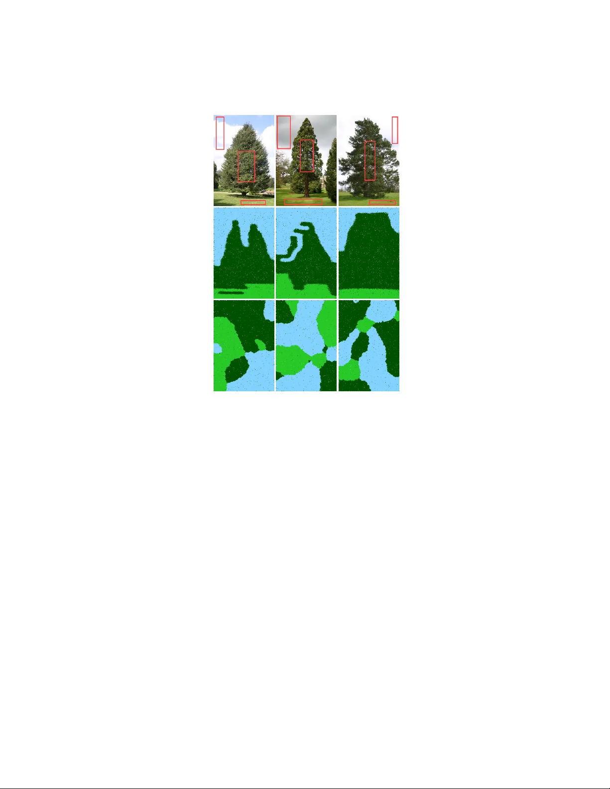
Modelling Distrib uted Shape Priors by Gibbs Random Fields of Second Order Boris Flach 1 and Dmitrij Schlesinger 2 1 Center for Machine Perception, Czech T echnical Univ ersity in Prague 2 Institute for Artificial Intelligence, Dresden Univ ersity of T echnology Abstract. W e analyse the potential of Gibbs Random Fields for shape prior mod- elling. W e sho w that the e xpressiv e po wer of second order GRFs is already suf fi- cient to express simple shapes and spatial relations between them simultaneously . This allows to model and recognise comple x shapes as spatial compositions of simpler parts. 1 Introduction Motivation and goals Recognition of shape characterist ics is one of the major aspects of visual information processing. T ogether with colour, motion and depth processing it forms the main pathways in the visual cortex. Experiments in cognitiv e science show in a quite impressiv e way , that humans recognise comple x shapes by decomposition into simpler parts and interpreting the for- mer as coherent spatial compositions of these parts [6]. Corresponding guiding prin- ciples for the decomposition where identified from these experiments as well as from research in computer vision (see e.g. [8]). The formulation of these principles relies howe ver on the assumption that the objects are already segmented and thus concepts like con vexity and curv ature can be applied. From the point of view of computer vision it is desirable to use shape processing and modelling in the early stages of visual processing. This allows to control e.g. se gmen- tation directly by prior assumptions or by feedback from higher processing layers. This leads to the question whether composite shape models can be represented and learned in a topologically fully distributed w ay . The aim of the presented work is to study this question for probabilistic graphical models. Related work All mathematically well principled shape models for early vision can be roughly divided into the follo wing two groups. Global models treat shapes as a whole. Prominent representati ves are variational models and le vel set methods in particular . A shape is described up to its pose by means of a lev el set function defined on the image domain. Cremers et.al. have sho wn in [2] how to extend these models for scene segmentation. Recently we have sho wn how to use level set methods in conjunction with MRFs [3]. Global shape models are well suited e.g. for segmentation and tracking if the number of objects is kno wn in adv ance and a good initial pose estimation is provided. 2 Boris Flach and Dmitrij Schlesinger Semi global models consider shape characteristics in local neighbourhoods and go back to the ideas of G. Hinton on “product of experts” as well as of Roth and Black on “fields of experts” (see [5, 10] and citations therein). Mathematically these models are higher order GRFs of a certain type – additional auxiliary variables are used to express mixtures of local shape characteristics in usually overlapping neighbourhoods. Marginalisation over these auxiliary variables results in GRFs of higher order . The work of K ohli, T orr et.al. [9, 7] demonstrates how to introduce such higher order Gibbs po- tentials directly and to use them for segmentation in hierarchical Conditional Random Fields (CRF). Ho wev er, it is not clear ho w to learn the graphical structure for such models. Contributions W e will sho w that Gibbs Random Fields of second order hav e already sufficient expressi ve power to model complex shapes as coherent spatial compositions of simpler parts. Obviously , these models have to hav e a significantly more complex graphical structure than just simple lattices. Moreov er, the graphical structure itself be- comes a parameter which has to be learnt together with the Gibbs potentials for each considered shape class. From the application point of view these models ha ve advantages especially in the context of scenes with an unkno wn number of similar objects (i.e. all objects are in- stances of a single shape class). Moreover , such models can be easily combined for scenes with instances of different shape classes. The structure of the paper is as follows. In section 2 we introduce the GRF model for composite shapes and discuss the inference and learning tasks. The latter means to learn the Gibbs potentials and the graphical structure itself. Section 3 giv es experiments exploring the expressiv e power of the model – first we separately show its ability to express spatial relations between segments and its ability to model simple shapes. Then we demonstrate its capability to model composite shapes including structure learning. Finally , we sho w how to combine such models for the discrimination of shape classes. 2 The shape model Probability distribution W e begin with the description of the prior part of our shape model. Let D ⊂ Z 2 be a finite set of nodes t ∈ D , where each node corresponds to an image pixel. Let A ⊂ Z 2 be a set of vectors used to define a neighbourhood structure on the set of nodes, i.e. a graph: two nodes t and t 0 are connected by an edge if t 0 − t = a ∈ A . T o avoid double edges we require − A ∩ A = 0 (we use unary potentials as well). The resulting graph is obviously translational in variant and the elements of a ∈ A define subsets E a ⊂ E of equi v alent edges, where e = ( t, t 0 ) ∈ E a if t 0 − t = a . A simple example is sho wn in Fig. 1. Giv en a class of composite shapes, we denote the set of its parts enlar ged by an e xtra element for the background by K . A shape-part labelling y : D → K is a mapping, that assigns either a shape-part label or the background label y t ∈ K to each node t ∈ D . A function u a : K × K → R is defined for each difference vector a ∈ A . Its values u a ( k , k 0 ) are called Gibbs potentials. A corresponding probability distrib ution is Modelling Shape Priors by GRFs 3 u a ( k , k 0 ) t t 0 Background label Part-shape labels e ∈ E a Fig. 1. Left: example of a translational inv ariant graphical structure. Equiv alence classes of edges E a are coloured by different colours. The set A is represented by bold edges outgoing from the central node. Right: Gibbs potentials for an edge from E a . defined ov er the set of shape-part labellings as follo ws p ( y ) = 1 Z ( u ) exp X a ∈ A X tt 0 ∈ E a u a  y t , y t 0  , (1) where Z denotes the partition sum (we omit the unary terms for better readability). This p.d. is homogeneously parametrised – all edges in an equiv alence class E a hav e the same potentials. Remark 1. Note that the parameters u a of this model are unique up to additiv e constants for a giv en p.d. under fairly general assumptions – the only possible equiv alent trans- formations (aka re-parametrisations) consist in adding a constant ˜ u a () = u a () + const. This will be sho wn in appendix A. Therefore, we assume from here that the Gibbs potentials for each a ∈ A are normalised to sum to zero: P k,k 0 u a ( k , k 0 ) = 0 . Remark 2. It is important to notice that a homogeneously parametrised GRF on a finite domain D ⊂ Z 2 is not necessarily homogeneous. A p.d. p ( y ) for labellings y : D → K is called homogeneous if its marginals for congruent subsets coincide. This inhomo- geneity , if present, usually re veals at the domain boundary . It is easy to verify that the con verse is true at least for chains: a homogeneous Marko v model on a finite chain admits a homogeneous parametrisation. The appearance model is assumed to be a “simple” conditional independent model. The probability to observe an image x : D → C ( C is some colour space) giv en a shape-part labelling y is p ( x | y ) = Y t ∈ D p  x t | y t  . (2) In the light of the current popularity of CRFs it might well be asked, why we decided to fa vour a GRF here. Both v ariants are identical with respect to inference. Differences occur for learning. W e can imagine that shape-part labellings can be used as latent variable layers for complex object segmentation models. Recently , empirical risk min- imisation learning has been proposed for structured SVM models with latent variables 4 Boris Flach and Dmitrij Schlesinger [13]. This sho ws that learning of graphical models with latent variables is possible for both v ariants – GRFs and CRFs. Howe ver , since we want to study the e xpressi ve power of the model in its pure form, we need a prior p.d. and moreover , we want to be able to learn such models fully unsupervised, which is possible for GRFs but not for CRFs. The inference task Informally , the inference task can be understood as follows. Giv en an observation (i.e. an image), it is necessary to assign values to all hidden v ariables. W e pose the segmentation task as a Bayesian decision task. Let y 0 be the true (but unknown) segmentation and C ( y , y 0 ) be a loss function, that assigns a penalty for each possible decision y . The task of Bayesian decision is to minimise the e xpected loss R ( y ; x ) = X y 0 p ( y 0 | x ) C ( y , y 0 ) → min y . (3) W e use the number of misclassified pixels C ( y , y 0 ) = X t 1 I  y t 6 = y 0 t  (4) as the loss function. It leads to the max-marginal decision y ∗ t = max k p  y t = k   x  ∀ t ∈ D . (5) Hence, it is necessary to calculate the marginal posterior probabilities for each node t ∈ D and label k ∈ K . Currently this task is infeasible for GRFs. Several approx- imation techniques based e.g. on belief propagation or variational methods hav e been proposed for this task (see e.g. [12] for an overvie w). Unfortunately none of them guar- antees conv ergence to the exact values of the sought-after mar ginal probabilities. T o our knowledge, the only scheme which does it is sampling, which is howe ver known to be slow [11]. Estimation of Gibbs potentials The learning task comprises to estimate the unknown model parameters gi ven a learning sample. W e assume that the latter is a random realisa- tion of i.i.d. random variables, so that the Maximum Likelihood estimator is applicable. The following situations are distinguished depending on the format of the learning data. If the elements of the sample hav e the format ( x, y ) then the learning is called supervised . If, instead, they consist of images only then the learning is called fully unsupervised. T o cope with variants in-between as well, i.e. partial labellings y V , we consider the elements of the training sample to be ev ents of the type B = ( x, y V ) = { ( y , x ) | y | V = y V } . W e start with the learning of unknown potentials u . For simplicity we consider the case when only one ev ent B is giv en as the training sample. According to the Maximum Likelihood principle, the task is p ( B ; u ) = X y ∈B p ( y ) p ( x | y ) → max u . (6) Modelling Shape Priors by GRFs 5 T aking the logarithm and substituting the model (1), (2) giv es L ( u ) = log X y ∈B exp h X a ∈ A X tt 0 ∈ E a u a  y t , y t 0  i p ( x | y ) − log  Z ( u )  → max u . (7) It is easy to prove, that the deri v ativ e with respect to the potentials is a difference of expectations of some random variable n a ( k , k 0 ; y ) with respect to the posterior and prior p.d. ∂ L/∂ u a ( k , k 0 ) = E p ( y |B ; u ) [ n a ( k , k 0 ; y )] − E p ( y ; u ) [ n a ( k , k 0 ; y )] . (8) The random variables n a ( k , k 0 ; y ) are defined by n a ( k , k 0 ; y ) = X tt 0 ∈ E a 1 I  y t = k , y t 0 = k 0  (9) and represent co-occurrences for label pairs ( k , k 0 ) along the edges in E a for a labelling y . Combining these random variables into a random vector Φ , the gradient of the log- likelihood can be written as ∇ L ( u ) = E p ( y |B ; u ) [ Φ ] − E p ( y ; u ) [ Φ ] . (10) The exact calculation of the expectations in (8) is not feasible. Therefore, we pro- pose to use a stochastic gradient ascent to maximise (7). The learning algorithm is an iteration of the following steps: 1. Sample ˜ y and y according to the current a-posteriori probability p ( y |B ; u ) and a- priori probability p ( y ; u ) respecti vely . 2. Compute n a ( k , k 0 ; ˜ y ) and n a ( k , k 0 ; y ) by (9) for each a ∈ A , k , k 0 ∈ K . 3. Replace the e xpectations in (8) by their realisations and calculate ne w potentials u . For the sake of completeness we would like to mention that the learning of the appearance models p ( c | k ) can be done in a v ery similar manner . It is e ven simpler from the computational point of vie w because the normalising constant Z does not depend on these probabilities. Therefore it is not necessary to sample labellings according to the a-priori probability distribution p ( y ) . Only a-posteriori sampled labellings are needed to perform the corresponding stochastic gradient step. Estimation of the interaction structure A very important question not discussed so far is the optimal choice of the neighbourhood structure A . Unfortunately , no well founded answer to this question is kno wn at present. One option is to use an abun- dant set of interaction edges, e.g. to assume that the set A consists of all vectors A = { a ∈ Z 2 | | a 1 | , | a 2 | 6 d } within a certain range. Despite of the computational com- plexity this would lead to models with high VC dimension and possibly – as a result – to weak discrimination. It is therefore important to in vestigate the possibility to iden- tify the neighbourhood structure A from a giv en training sample. A possible variant of a corresponding formal task reads as follows. Giv en a training sample the task is to find the best neighbourhood structure A of given size | A | = m according to the 6 Boris Flach and Dmitrij Schlesinger Maximum Likelihood principle L ( u A , A ) → max u A ,A . This task is howe ver not fea- sible - an exhausti ve search over all possible sets A would be computationally pro- hibitiv e, and, moreover , the likelihood can be calculated only approximatively . There- fore we rely on a greedy approximation which we will consider in two variants – one of them successively includes new elements into the neighbourhood structure starting from A = { 0 } and the other successi vely remov es elements from this structure starting from A = { a ∈ Z 2 | | a 1 | , | a 2 | 6 d } . For the first v ariant we use a greedy search for the interaction edges proposed by Zalesny and Gimel’farb in the context of texture modelling [14, 4]. Starting from the set A = { 0 } , i.e. a model with unary potentials, new edges are iterati vely chosen and included into A as follows. First, the optimal set of potentials u ∗ A ∈ U A is determined for the current set A as described in the previous subsection. Here U A denotes the subspace of potentials on the edges in A (we may assume that the Gibbs potentials are zero on all other edges). If a bigger neighbourhood A 0 is considered, then clearly , the gradient of the (log) likelihood with respect to u A 0 in the point u ∗ A will be orthogonal to the subspace U A . The proposal is to include the vector a 0 ∈ A 0 \ A with the largest gradient component a 0 = arg max a ∈ A 0 \ A X k,k 0  n a ( k , k 0 ; B , u ) − n a ( k , k 0 ; u )  2 (11) Optionally the Kullback-Leibler div ergence can be used instead of the Euclidean dis- tance. The second v ariant of structure estimation proceeds in opposite order . Starting with the neighbourhood structure A = { a ∈ Z 2 | | a 1 | , | a 2 | 6 d } , elements of A are succes- siv ely removed. The aim is to remo ve in each step the element with the smallest impact on the maximal likelihood max u A L ( u A ) − max u A \ a L ( u A \ a ) → min a ∈ A . (12) It is impossible to estimate this expression in the point u ∗ A = arg max u A L ( u A ) using the gradient of the likelihood (like in the first variant) because of ∇ L ( u ∗ A ) = 0 . It is nev ertheless possible to estimate this expression based on u ∗ A . For the sake of simplicity we sho w this for the situation of supervised learning. The lik elihood maximisation with respect to the Gibbs potentials reads max u A n h ψ A , u A i − log X y exp h φ A ( y ) , u A i o (13) for this case. Here we have used the follo wing notations. The set of all Gibbs potentials u a ( ., . ) , a ∈ A is considered as a vector u A . A realisation of the random vector Φ A (see (10)) is denoted by φ A ( y ) . Finally , ψ A denotes the corresponding vector of statistics resulting from the training sample. Designating log Z ( u A ) by H ( u A ) , the expression in (13) is nothing but the Fenchel conjugate H ∗ ( ψ A ) . It is known that for exponential families the latter can be written as H ∗ ( ψ A ) = inf n X y p ( y ) log p ( y )    E p [ Φ A ] = ψ A , p ∈ P o (14) Modelling Shape Priors by GRFs 7 (see e.g. [12, 1]), where we denoted the expectation w .r .t. a probability distribution p by E p and the set of all probability distributions on labellings y by P . This means to find the p.d. with maximal entropy among all distrib utions having expectation ψ A of the random vector Φ A . Removing an element a from the neighbourhood structure A can be equiv alently expressed by the linear constraints u a ≡ 0 . Considering the task (13) with these addi- tional constraints, it can be shown by the use of Fenchel duality (see e.g. [1]) that the corresponding conjugate function e H ∗ ( ψ A ) can be written as e H ∗ ( ψ A ) = inf z a inf p n X y p ( y ) log p ( y )    E p [ Φ A ] = ψ A + z a , p ∈ P o , (15) where z a is an arbitrary vector of the subspace U a . Therefore, the difference in (12) is equal to H ∗ ( ψ A ) − e H ∗ ( ψ A ) = H ∗ ( ψ A ) − H ∗ ( ψ A + z ∗ a ) and can be estimated by the gradient of H ∗ in ψ A . The latter gradient is nothing but the vector of Gibbs potentials u ∗ A . Remark 3. The con ve x, lower semi-continuous function H ∗ ( ψ A ) is not dif ferentiable in general. Therefore its sub-differential may consist of more than one subgradient u A . This corresponds to the non-uniqueness of the Gibbs potentials. W e ha ve how- ev er shown that the Gibbs potentials are unique up to additi ve constants for the model class considered in this paper (see Remark 2 and Appendix A). Summarising, the dif ference in (12) can be estimated by k u a k , what leads to the fol- lowing greedy remov al strategy for elements of the neighbourhood structure A . Giv en a current neighbourhood structure A , estimate the optimal Gibbs potentials u ∗ A and re- mov e the the element a ∈ A with the smallest v alue of k u a k . 3 Experiments Modelling spatial relations between segments The first experiment in vestigates the ability of the model (1), (2) to reflect spatial relations between segments, i.e. scene parts, which are too large to capture their shape by a neighbourhood structure of reasonable size. W e used the three images sho wn in the first row of Fig. 2 as training examples. Each scene should be segmented into three segments: K = { sky , tr ees, g r ass } . The appearance models p ( c | k ) for the segments were assumed as mixtures of multi variate Gaussians (four per segment). A model with ”full“ neighbourhood structure – all vec- tors { a ∈ Z 2 | | a 1 | , | a 2 | ≤ d } with d = 20 was used in this experiment. A “simple” b ut anisotropic Potts model on the 8-neighbourhood was chosen as a baseline for compari- son. Semi-supervised learning was applied by fixing the segment labels in the rectangu- lar areas shown by red rectangles during learning. Both the a-priori models (the poten- tials and the direction specific Potts parameters for the baseline model) and the appear - ance models (mixture weights, mean values and co variance matrices) were learned. The difference of the models can be clearly seen by observing labellings generated a-priori by the learned models, i.e. without input images. Some of them are shown in the 8 Boris Flach and Dmitrij Schlesinger Fig. 2. Modelling spatial relations between segments. The first row shows input images and re- gions with fixed segmentation. The middle and bottom row show labellings generated by the learned a-priori models (se gment labels are coded by colour): the images in the middle ro w were generated by the model with full neighbourhood, whereas the images in the bottom ro w were generated by the baseline model. second and third row for the model with complex neighbourhood structure and the base- line model respecti vely . It can be seen, that the spatial relations between segments (like e.g. “abov e”, “belo w” etc.) were correctly captured by the complex model, whereas it is clearly not the case for the Potts model. The consequences can be clearly seen from the following experiment. W e fixed the prior models obtained in the previous experiment (semi-supervised learning) for both variants (the complex prior and the Potts prior) and learned the parameters of the Gaus- sian mixtures completely unsupervised. Fig. 3 shows labellings (i.e. segmentations) sampled at the end of the learning process by the corresponding a-posteriori probabil- ity distributions (obtained with the learned appearances) for the complex a-priori model and the Potts a-priori model in the first and the second row respectiv ely . The advantages of the complex model are clearly seen. These results can be explained as follo ws. There are twelv e Gaussians in total to interpret the gi ven images. For the learning process it is “hard to decide” which of the Gaussians belongs to which segment. Using the compact- Modelling Shape Priors by GRFs 9 Fig. 3. Se gmentation results obtained after fully unsupervised learning of the appearance part of the model. Upper row – model with full neighbourhood, bottom ro w – baseline model. ness assumption only , is obviously not enough to separate segments from each other . If the complex model is used instead, the learning process starts to generate labellings according to the a-priori probability distrib ution, i.e. labellings which reflect the correct spatial relations between the segments. This forces the unsupervised learning of the appearance models into the right direction. Modelling simple shapes This group of experiments demonstrates the ability of the model to represent simple shapes as well as to perform shape driv en segmentation. This experiment is prototypical e.g. for a class of image recognition tasks in biomedical re- search. Fig. 4 (upper left) sho ws a microscope image of liver cells with stained DNA. Thus, only the cell nuclei are visible. The task is to segment the image into two seg- ments – ”cells“ (which hav e nearly circular shape) and ”background“ (the rest including artefacts). Hence, two labels are used. The ”full“ neighbourhood structure with d = 12 was used (it approximately corresponds to the mean cell diameter). Again, we used a baseline model for comparison – a GRF with 4-neighbourhood and free potentials. The appearances for grey-v alues were assumed to be Gaussian mixtures (two per segment) in both models. First, semi-supervised learning was performed (lik e in the previous experiment with trees) in order to learn the prior distributions for labellings as well as the appearances for both, the complex and the baseline model. A labelling generated a-priori by the learned complex model is shown in Fig. 4 (upper right). The final segmentations according to the max-marginal decision (see equation (5)) are shown in the bottom row of the same 10 Boris Flach and Dmitrij Schlesinger Fig. 4. Modelling and segmentation of simple shapes. Upper left – input image, upper right – a labelling generated a-priori by the learned complex model. Final segmentations are sho wn in the bottom row: left – baseline model, right – comple x model. figure. The differences are clearly seen. The shape prior captured in the complex model led to the correct segmentation – the artefacts were se gmented as background, whereas the baseline model produces a wrong segmentation because neither the appearance nor a simple ”compactness“ assumption nor e ven their combination allo w to differentiate between cells and artefacts. Structure estimation f or simple shapes In order to in vestigate the structure iden- tifiability of shape models we have used an artificial model which generates simple ”blobs“. The neighbourhood structure consists of 8 elements. The group of the first four elements with coordinates (0 , 1) , (0 , − 1) , (1 , 1) and ( − 1 , 1) describes a standard 8-neighbourhood. The remaining four vectors are scaled v ersions of the first (scale fac- tor 5). The Gibbs potentials on the short vectors are supermodular and express the cor- relation of the labels on the edges of this type u ( k , k 0 ) = ( α if k = k 0 , − α else. . (16) The Gibbs potentials on the long edges consist of an submodular and a modular part u ( k , k 0 ) = u 1 ( k , k 0 ) + u 2 ( k , k 0 ) , where the submodular part u 1 is just the negati ve version of the potentials on the short edges and expresses an anti-correlation of the labels on these edges. The modular part u 2 ( k , k 0 ) =      β if k = k 0 = 0 , − β if k = k 0 = 1 , 0 else . (17) Modelling Shape Priors by GRFs 11 Fig. 5. Shape estimation for a simple shape model. Left – labelling generated by the known model, right – histogram of the estimated structures. is used to influence the density of the blobs. A labelling (fragment) sampled by this model ( α = 0 . 35 , β = 0 . 5 ) is sho wn in Fig. 5. Both heuristic approaches for structure estimation discussed in the previous section where applied for the supervised version, i.e. using a labelling generated by the known model as a learning sample. The first approach – iterativ e gro wth of the structure – was run 40 times. The es- timated structures resulting from these runs are shown in Fig. 5 as a grey-coded his- togram. As a stochastic gradient ascend is used for the learning of the potentials, each run may result in a dif ferent structure. The histogram shows ho wever , that the structure estimation is essentially correct. All trials of the second approach – iterative shrinking of the neighbourhood structure – resulted much to our surprise in one and the same estimated structure – the correct one. W e conclude from these experiments that the neighbourhood structure of a shape model is identifiable (at least in principle) from labellings generated by the model. Modelling composite shapes The pre vious experiments ha ve sho wn that second order GRFs can model both, spatial relations between segments and simple shapes. No w we are going to demonstrate the capability of the model to capture both properties simulta- neously . This opens the possibility to represent comple x shapes as spatial compositions of simpler parts. T o demonstrate this, we use an artificial example shown in Fig. 6 (up- per left). It was produced manually and corrupted by Gaussian noise. Accordingly , the model was defined as follo ws. The label set K consists of sev en labels, each one cor- responding to a part of the modelled shape (as well as one for the background). The appearance models p ( c | k ) for the labels are Gaussians with kno wn parameters. In this experiment we applied the gro wth v ariant for the estimation of the interaction structure as described in section 2. Fig. 6 (upper row , center) shows a labelling generated by the learned prior model. It is clearly seen that both, spatial relations between object parts and part shapes are captured correctly . The bottom row of Fig. 6 displays labellings generated during the process of struc- ture learning at time moments, when the interaction structure learned so far was not yet capable to capture all needed properties. As it can be seen, the model was able to 12 Boris Flach and Dmitrij Schlesinger Fig. 6. Composite shape modelling. Upper row from left: input image, labelling generated a- priory by the learned model, estimated interaction structure. Bottom row: labellings generated by models during learning. learn spatial relations between the segments more or less correctly even for a small numbers of edges ( 5 edges – bottom left). More relations are learned as the number of edges grows (bottom middle and right). Finally , 20 difference vectors were necessary to capture all relations (out of 1200 possible for the maximal range of d = 24 ). Fig. 6 (upper right) sho ws the estimated neighbourhood structure. The endpoints of all edges from central pixel are marked by colours (the image is magnified for better visibility). A certain structure can be seen in this image. The 8 -neighbourhood edges (black) reflect compactness and adjacenc y relations of the object parts. The learned po- tentials on these edges represent strong label co-occurrences. Most of the other vectors are responsible for the shapes of the parts. The potentials on the red edges express char- acteristic breadths, and the potentials on the green edges – characteristic lengths of the parts. The potentials on these edges mainly represent anti-correlations, forcing label values to change along certain directions. The blue pixels in the figure reflect relative positions of object parts. Composite shape recognition The final experiment demonstrates possibilities to com- bine composite shape models. The aim is to obtain a joint model which can be used for detection, segmentation and classification of objects in scenes populated by instances of different shape classes like e.g. the example in Fig. 7. W e conclude from the pre vious experiments, that the appearance model can be re-learned in a fully unsupervised way if the prior shape model is discriminativ e. Hence, the most important question is, ho w to combine the prior models. W e propose a method for this that is based on the following observation. It is not necessary to hav e an example image (or an example segmentation) Modelling Shape Priors by GRFs 13 Fig. 7. Shape segmentation and classification. Left – input image, right – segmentation (part- labels are encoded by colours). in order to learn the model if the aposteriori statistics ¯ Φ a ( k , k 0 ) = E p ( y |B ,u )  Φ a ( k , k 0 )  (18) for all dif ference vectors a ∈ A and label pairs ( k , k 0 ) are known – the gradient of the likelihood (equation (8)) reads then ∂ L/∂ u a ( k , k 0 ) = ¯ Φ a ( k , k 0 ) − E p ( y ; u ) [ n a ( k , k 0 ; y )] . (19) Let us consider this in a bit more detail for a simple example – just two shapes like in Fig. 7. Let us assume that the both models are learned, i.e. both the potentials and statistics are known for both models and for all difference vectors a . Obviously , it is not easy to combine the potentials of both shape models in order to obtain new ones for a model that generates such collages. It is howe ver very easy to estimate the needed aposteriori statistics for the joint model giv en the aposteriori statistics for both shape models. Summarizing, the scheme to obtain the parameters of the joint model consists of two stages: 1. compute the aposteriori statistics for the joint model and 2. learn the model according to (19) so that it reproduces this statistics. As the second stage is standard, we consider the first one in more detail. Let us denote the label sets corresponding to the shape parts by K 1 and K 2 for the first and for the second shape type respectively . Let b 1 and b 2 be the background labels in the corre- sponding shape models and b be the background label in the joint one. Consequently , the label set of the latter is K 1 ∪ K 2 ∪ b (see the middle part of Fig. 8). First of all we enlar ge the label sets of each shape model by labels that are not present in this model but present in the joint one. Thereby the statistics for the new introduced labels (for all difference vectors a ) are set to zero (see Fig. 8, left and right). Informally said, these extended aposteriori statistics correspond to the situations that the joint model is learned on examples, in which only labels of one particular shape are present. The aposteriori statistics for the joint model is then obtained as a weighted 14 Boris Flach and Dmitrij Schlesinger K 2 K 1 ⇒ b 1 ⇐ b 2 Fig. 8. Estimation of the aposteriori statistics for the joint model. Left and right: extended statis- tics for shape models. Middle: the joint model – statistics marked green and red are inherited from the components. Others are set to a small constant. mixture of the two extended ones and an additional uniformly distributed component. The latter is added in order to a void zero probabilities (which would lead to obvious technical problems for the Gibbs Sampler). Summarising, the aposteriori statistics of label pairs for a difference v ector a of the joint model is: ¯ Φ a ( k , k 0 ) ∼                            w 1 · ¯ Φ 1 a ( k , k 0 ) + w 0 if k ∈ K 1 and k 0 ∈ K 1 , k ∈ K 1 and k 0 = b, k = b and k 0 ∈ K 1 , w 2 · ¯ Φ 2 a ( k , k 0 ) + w 0 if k ∈ K 2 and k 0 ∈ K 2 , k ∈ K 2 and k 0 = b, k = b and k 0 ∈ K 2 , w 1 · ¯ Φ 1 a ( b 1 , b 1 )+ + w 2 · ¯ Φ 2 a ( b 2 , b 2 ) + w 0 if k = b and k 0 = b w 0 otherwise. (20) with some weights w 0  w 1 ≈ w 2 , where the indices 1 and 2 correspond to the particular shape model. Giv en these statistics the joint model is learned according to (19). For the experiment in Fig. 7 two composite shape models were learned separately . The test image in Fig. 7 (left) is a collage of both shape types. Note that the appearance of all shape parts is identical, so they are not distinguishable without the prior shape model. Fig. 7 (right) shows the final segmentation. It is seen that all objects were cor- rectly segmented and recognised – although both composite shape classes share some similarly shaped parts – they were not confused. 4 Conclusions The notation of shape is often understood as an object property of global nature. W e fol- lowed a different direction by modelling shapes in a distributed way . W e have demon- strated that the expressiv e power of second order GRFs allows to model spatial relations of segments, simple shapes and moreover , both aspects simultaneously i.e. composite shapes which are understood as coherent spatial compositions of simpler shape parts. Modelling Shape Priors by GRFs 15 W e have sho wn that complex shapes can be recognized ev en in the situation, when their parts are not distinguishable by appearance. Howe ver , in our learning experiments we used training images, where they are distinguishable. Thus, an important question is, whether it is possible to perform unsupervised decomposition of complex shapes into simpler parts during the learning phase, i.e. to learn shape models from images, where the desired spatial relations between shape parts are not e xplicitly present. Another important issue is the learning of the interaction structure. It would be very useful to hav e a well grounded approach for this. Acknowledgments W e w ould like to thank Geor gy Gimel’farb (Uni versity of Auckland) for the fruitful and instructiv e discussions which have been particularly v aluable with regard to structure learning. One of us (B.F .) was supported by the Czech Ministry of Education project 1M0567. D.S. was supported by the Deutsche Forschungsgemeinschaft, Grant FL307/2-1. Both authors were partially supported by Grant NZL 08/006 of the Federal Ministry of Edu- cation and Research of Germany and the Royal Society of Ne w Zealand. References 1. Borwein, J.M., Lewis, A.S.: Con vex Analysis and Nonlinear Optimization. No. 3 in CMS Books in Mathematics, Springer (2000) 2. Cremers, D., Sochen, N., Schnörr , C.: A multiphase dynamic labeling model for variational recognition-driv en image segmentation. IJCV 66(1), 67–81 (January 2006) 3. Flach, B., Schlesinger , D.: Combining shape priors and MRF-segmentation. In: da V itoria Lobo et al., N. (ed.) S+SSPR 2008. pp. 177–186. Springer (2008) 4. Gimel’farb, G.L.: T exture modeling by multiple pairwise pixel interactions. IEEE T rans. Pattern Anal. Mach. Intell. 18(11), 1110–1114 (1996) 5. Hinton, G.E.: T raining products of experts by minimizing contrastive di ver gence. Neural Computation 14(8), 1771–1800 (2002) 6. Hoffman, D.D.: V isual Intelligence: How W e Create What W e See. W . W . Norton & Com- pany (2000) 7. Ladicky , L., Russell, C., Kohli, P ., T orr , P .H.: Associativ e hierarchical crfs for object class image segmentation. In: Proceedings IEEE 12. International Conference on Computer V ision (2009) 8. Liu, H., Liu, W ., Latecki, L.J.: Conv ex shape decomposition. In: CVPR. pp. 97–104 (2010) 9. Ramalingam, S., K ohli, P ., Alahari, K., T orr , P .: Exact inference in multi-label CRFs with higher order cliques. In: CVPR 2008. pp. 1–8 (June 2008) 10. Roth, S., Black, M.J.: Fields of experts. International Journal of Computer V ision 82(2), 205–229 (2009) 11. Sokal, A.D.: Monte carlo methods in statistical mechanics: Foundations and ne w algorithms. Lectures notes (1989) 12. W ainwright, M.J., Jordan, M.I.: Graphical models, exponential families, and variational in- ference. Foundations and T rends in Machine Learning 1(1–2), 1–305 (2008) 13. Y u, C.N.J., Joachims, T .: Learning structural svms with latent variables. In: International Conference on Machine Learning (ICML) (2009) 16 Boris Flach and Dmitrij Schlesinger 14. Zalesny , A., Gool, L.V .: Multivie w texture models. In: Proceedings of the IEEE Conference on Computer V ision and Pattern Recognition 2001. pp. 615–622. IEEE Computer Society (2001) A Equivalent transforms for homogeneously parametrised GRFs As we ha ve already seen, the probability distrib ution (1) for shape part labellings y can be equiv alently written as p ( y ) ∼ exp h X k u 0 ( k ) n 0 ( k ; y ) + X a ∈ A 0 X kk 0 u a ( k , k 0 ) n a ( k , k ; y ) i , (21) where A 0 = A \ { 0 } . W e call two parametrisations u , ˜ u equiv alent, if the correspond- ing probability distributions are identical. It follows that the difference v = u − ˜ u of equiv alent potentials fulfils V ( y ) = X k v 0 ( k ) n 0 ( k ; y ) + X a ∈ A 0 X kk 0 v a ( k , k 0 ) n a ( k , k 0 ; y ) = const. (22) W e will conclude that all functions v a are constant under fairly general conditions. W e perform the proof in two steps. First we sho w that the pairwise functions v a , a 6 = 0 are modular and can be written as a sum of unary functions. In a second step we will conclude the claimed statement under fairly general conditions for the graph ( D, E ) . Let us consider an arbitrary non-zero vector a ∈ A of the neighbourhood structure and an arbitrary edge ( tt 0 ) ∈ E a . Let k 1 , k 2 be two arbitrary labels in the node t and k 0 1 , k 0 2 be two arbitrary labels in the node t 0 . Let y 11 , y 12 , y 21 , y 22 be four labellings with respective values ( k 1 , k 0 1 ) , ( k 1 , k 0 2 ) , ( k 2 , k 0 1 ) , ( k 2 , k 0 2 ) on the nodes t, t 0 such that they coincide on all other v ertices. W e consider the equation V ( y 11 ) + V ( y 22 ) − V ( y 12 ) − V ( y 21 ) = 0 . (23) It is easy to see that this equation reduces to v a ( k 1 , k 0 1 ) + v a ( k 2 , k 0 2 ) − v a ( k 1 , k 0 2 ) − v a ( k 2 , k 0 1 ) = 0 . (24) This holds for arbitrary four-tuples of labels and it follows that the function v a is mod- ular and can be written as a sum of two unary functions v a ( k , k 0 ) = ˜ v a ( k ) + ˜ v − a ( k 0 ) . (25) These arguments can be applied for every element a ∈ A 0 . Consequently , V ( y ) can be written as V ( y ) = X k v 0 ( k ) n 0 ( k ; y ) + X a ∈ A 0 X k  v a ( k ) n a ( k ; y ) + v − a ( k ) n − a ( k ; y )  , (26) where we hav e omitted the tildes. Note that n a ( k ; y ) = P k n a ( k , k 0 ; y ) denotes the number of vertices with an outgoing edge of type a for which the labelling y has the value k . Therefore in general n 0 ( k ; y ) 6 = n a ( k ; y ) . Modelling Shape Priors by GRFs 17 Let us consider an arbitrary verte x t and two labellings y , ˜ y which coincide on all vertices b ut t . It follo ws from V ( y ) − V ( ˜ y ) = 0 that v 0 ( k ) + X a ∈ A 0 t + a ∈ D v a ( k ) + X a ∈ A 0 t − a ∈ D v − a ( k ) = const. (27) W e assign a vector z ( t ) with dimension 2 | A | − 1 to every verte x t ∈ D with components z 0 ( t ) = 1 , z a ( t ) = ( 1 if t + a ∈ D , 0 else and z − a ( t ) = ( 1 if t − a ∈ D , 0 else. (28) If the domain D contains a subset of nodes t such that their vectors z ( t ) span the whole vector space of dimension 2 | A | − 1 , then, clearly , considering equation (27) for each of them, we obtain v 0 ( k ) = const. (29) v a ( k ) = const. (30) v − a ( k ) = const. (31) for all a ∈ A . u t