Discrete Calculus of Variations for Quadratic Lagrangians. Convergence Issues

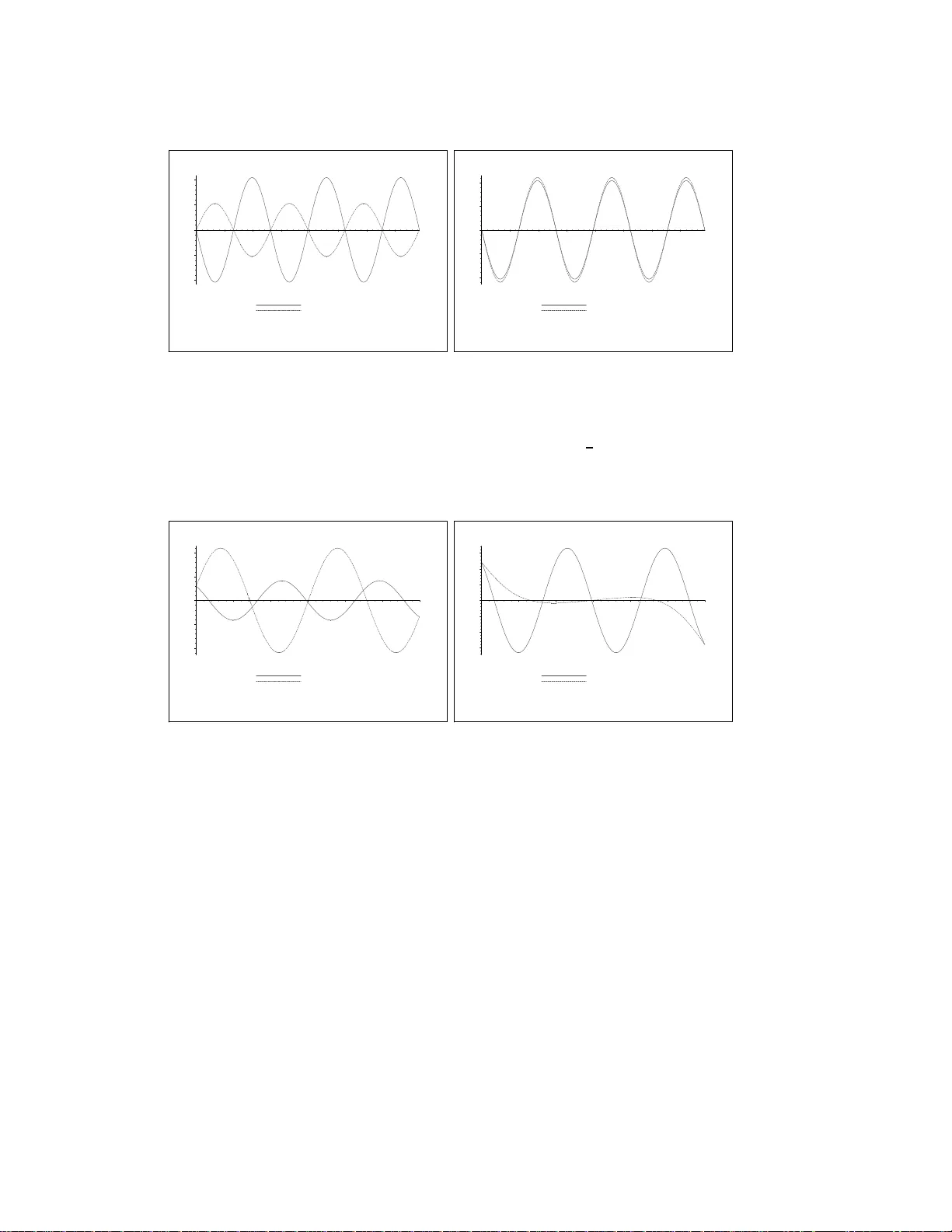
1 DISCRETE CALCULUS OF V ARIA TIONS FOR QUADRA TIC LA GRANGIANS. CON VER GENCE ISSUES PHILIPPE R YCKEL YNCK ∗ LAURENT SMOCH ∗ Abstract. W e study in this paper the contin uous and discrete Euler-Lagrange equations aris- ing from a quadratic lagrangian. Those equations may be though t as numerical sc hemes and ma y be solved through a matrix based framework. When the lagrangian is time-independent, we can solve both con tinuo us and discrete Euler-Lagrange equations under conv enien t oscil latory and non- resonance properties. Th e conv ergence of the solutions is also in vestiga ted. In the si m plest case of the harmonic oscillator, unconditional con vergence do es not hold, we giv e r esults and experiments in this dir ection. Key words. Calculus of v ariations, F unctional equations, Dis cretization, Boundary v alue prob- lems, Pseudo-p erio dic solutions. AMS sub ject classi fica tions. 49K21, 49K15, 65L03 , 65L12, 34K14 1. In tro duction. T he principle of least action may be extended to the case of no n- differentiable dynamical v ariables b y replacing in the lagrangian L ( x , ˙ x ) the deriv a tive ˙ x ( t ) of the dynamical v ariable x ( t ) with a 2 N + 1-terms scale deriv a tive  ε x ( t ) = N X i = − N c i x ( t + iε ) χ − i ( t ) , t ∈ [ a, b ] , (1.1) see [3, 4, 6 ]. Here, ε stands fo r some time delay and χ i ( t ) denotes the characteristic function of the interv al [ma x( a, a + iε ) , min( b, b + iε )]. Critical p oints of classical actions are c hara cterized by the class ical E uler-Lag range equations ∇ x L − d/dt ∇ ˙ x L = 0. Similarly , we prov ed in [6] that the equations o f motion for discr e tized actions are ∇ x L +  − ε ∇ ˙ x L = 0 . (1.2) W e abbr e viate as C.E .L. and D.E.L. the class ic al and discrete Eule r -Lagr ange sys tems of equatio ns resp ectively . In this paper we work with lagrangia ns of the shap e L ( x , ˙ x ) and L ( x ,  ε x ) where L : C d × C d → C is a quadratic p olynomia l. W e are interested in solving C.E .L. and D.E.L. under Dirichlet conditions. More a ccurately , w e study the existence and the unicit y of pseudo-p er io dic solutio ns z ( t ) of C.E.L. and y ε ( t ) of D.E.L., ε b eing fixe d. The underlying assumptions for this to o ccur may b e thought as a n “oscilla tory” con- dition for the lagrang ian L ( x , y ) and as a “non-reso nance” co ndition for the Dirichlet problem asso ciated to C.E.L. and D.E.L.. With this in mind, w e a ddress the problem of conv er g ence of y ε ( t ) to z ( t ). The pap er is org anized as follows. Sectio n 2 gives notation and basic definitio ns used thro ughout. In Section 3, we develop a matricial based framework to solve ∗ ULCO, LMP A, F-62100 Calai s , F rance. e-mail: { ryc kelyn,smoch } @lmpa.univ-littoral.fr Univ Lille Nord de F rance, F-59000 Lil le, F rance. CNRS, FR 2956 , F rance. 1 D.E.L. for all quadr atic time-dep endent lagrang ian. In Sectio n 4, we pr ovide under mild assumptions for m ulas for the compo ne nts of the pseudo-p erio dic solutions of C.E.L. and D.E.L. when the la grangia n doe s not explicitly dep end on time. This allows us to compute in some particular cases the phases of y ε ( t ) and z ( t ) help to the ma trix A . Section 5 is a preliminary discussion of conv ergence of y ε ( t ), uniformly lo cally in ] a, b [, as ε tends 0 for stationary lagrangia ns and pseudo -p erio dic solutions. If L is a non-resona nt osc illa tory lag rangia n and  ε is a w ell-chosen three-terms op erator , the prev ious co nvergence prop erty is the conten t o f o ur main theo rem which is proved in Section 6 . In Section 7, we give n umerica l exp eriments to illustra te the non-unconditional conv ergence of so lutions. 2. Preliminaries . Firs t, let us collect some notation and definitio ns from [6]. If the con text is clea r enough, i = √ − 1. Let [ a, b ] be some in terv a l of time and a time delay ε > 0 b e fixe d throughout. The integers d and N deno te resp ectively the “physical” dimension and the num ber of samples in C d . W e define for t 0 ∈ [ a, b ] the grid G t 0 ,ε = { t 0 + nε , n ∈ N } ∩ [ a , b ]. W e deno te by I d the identit y ma trix o f size d . Let C pw ( d, N ) b e the space of the fun ctions x : [ a, b ] → C d contin uous on eac h int erv al [ a + iε, a + ( i + 1) ε ] ∩ [ a, b ] for all i ∈ {− N , . . . , N } . The t wo functional spaces C 1 ([ a, b ] , C d ) and C pw ( d, N ) are Bana ch algebra s with uniform norms. The op erator  ε given in (1.1) is a contin uous linea r endomorphis m of C pw . Now, let b e g iven six mappings P, Q, J 1 ∈ C 1 ([ a, b ] , C d × d ), J 2 , J 3 ∈ C 1 ([ a, b ] , C d ) and J 4 ∈ C 1 ([ a, b ] , C ). W e suppo se that for all t , P ( t ) a nd Q ( t ) are symmetric and J 1 ( t ) is skew-symmetric. W e set L ( x , y ) = 1 2 t y P y + 1 2 t x Q x + t x J 1 y + t J 2 y + t J 3 x + J 4 . (2.1) and w e define the qua dratic la grangia ns L ( x , ˙ x ) and L ( x ,  ε x ). If the co e fficie nts in (2.1) do not depend explicitly on time, we shall say that L is sta tionary . W e will consider a ctions A cont ( x ) and A disc ( x ) of the shap e A cont ( x ) = Z b a L ( x , ˙ x )( t ) dt, A disc ( x ) = Z b a L ( x ,  ε x )( t ) dt. (2.2) The actions A cont : C 1 ([ a, b ] , C d ) → C and A disc : C pw ( d, N ) → C ar e contin uous and F r´ echet differen tiable everywhere. W e give in [6] the neces sary firs t o rder c o nditions of lo cal optimum of A cont and A disc under the Dirichlet constra ints x ( a ) = d a and x ( b ) = d b in the previo us spaces, where d a and d b are t wo fixed v ector s in C d . The Euler-Lagr ange equa tions asso ciated to each action in (2.2 ) c a n b e written as − P ¨ x + ( − ˙ P + 2 J 1 ) ˙ x + ( ˙ J 1 + Q ) x − ˙ J 2 + J 3 = 0 , (2.3)  − ε ( P  ε x ) −  − ε ( J 1 x ) + J 1  ε x + Q x +  − ε J 2 + J 3 = 0 . (2.4) 2 The problem of co nv ergence as ε tends to 0 of the o p e rator in the l.h.s. of (2.4) to the corresp onding op era tor in the l.h.s. of (2.3) has b een studied in [6]. In this context, w e in tro duced the class of discretization op erators given by  [ r,s ] ε x ( t ) = − χ +1 ( t ) s ε x ( t − ε ) + s − r ε x ( t ) + χ − 1 ( t ) r ε x ( t + ε ) . (2.5) where r , s ∈ C . In fact, (2.5 ) gives the sha pe of thre e -terms op erator s sa tisfying  ε (1)( t ) = 0 ins ide [ a + 2 ε, b − 2 ε ]. Without a ssuming the conv ergence of the schemes in the previous s e nse, we fo cus on the following t wo problems. Are the Dirichlet problems for (2 .3) and (2.4) well- po sed? Are there p er io dic or pseudo- p e r io dic solutions? In fact, if ε = ( b − a ) / M for some M ∈ N ⋆ and if x ε ( t ) is a solution of D.E.L ., then x ε is uniquely deter mined o n the grid G a,ε . W e shall see later how to co nstruct from x ε the unique cor resp onding pseudo-p erio dic solution y ε of (2.4). 3. An effectiv e metho d for solving D.E.L.. In this section, the datas N , d, L , d a , d b , ε ,  ε are fixed but arbitrar y . 3.1. D.E.L. as del a y ed functional equations. The eq uations (2.4) ma y be thought as a mixture betw een recurrence equations and delay ed functional equations. Let us transform the pr oblem of solving (2.4) into an infinit e set of pro blems, eac h of one dealing with r ecurrence vector equa tions with the additional difficult y of the per turbation of the b ounda ries. W e can identify e a ch function x : [ a, b ] → C d to the infinite set of finite sequences ( x ( t 0 + nε ) , n ∈ Z ) with indices such that a − t 0 ε ≤ n ≤ b − t 0 ε and where t 0 lies in an interv al o f length ε . In fact, b ecause (2.4 ) in volves the second o rder op era tor  − ε  ε , it may b e formu lated in an abstract manner as F ( t, x ( t − 2 N ε ) , x ( t − (2 N − 1) ε ) , . . . , x ( t + (2 N − 1) ε ) , x ( t + 2 N ε )) = 0 (3.1) where F : C 1+(4 N +1) d → C d contains the c o ordinates of the l.h.s. of (2.4). Hence, we solve (3.1) with r esp ect to x ( t 0 + 2 N ε ) for fixed t 0 , o r what a mounts to the same thing by expre s sing x ( t 0 + 4 N ε ) a s a function of x ( t 0 + k ε ) for k ∈ { 0 , . . . , 4 N − 1 } . F o r insta nce, the case N = 1 and d arbitrar y is the most interesting o ne, and w e may rewrite in this ca se the equations (2.4) as a sy stem of d equations x i ( t − 2 ε ) [ c 1 c − 1 χ 1 χ 2 P ij ( t − ε )] + x i ( t − ε ) [ c 0 c 1 χ 1 P ij ( t − ε ) + c 0 c − 1 χ 0 χ 1 P ij ( t ) + c 1 χ 1 ( J 1 ) j i ( t − ε ) + c − 1 χ 1 ( J 1 ) ij ( t )] + x i ( t ) [ c 2 1 χ 0 χ 1 P ij ( t − ε ) + c 2 0 χ 0 P ij ( t ) + c 2 − 1 χ 0 χ − 1 P ij ( t + ε ) + χ 0 Q ij ( t )] + x i ( t + ε ) [ c 0 c 1 χ 0 χ − 1 P ij ( t ) + c 0 c − 1 χ − 1 P ij ( t + ε ) + c 1 χ − 1 ( J 1 ) ij ( t ) + c − 1 χ − 1 ( J 1 ) j i ( t + ε )] + x i ( t + 2 ε ) [ c − 1 c 1 χ − 1 χ − 2 P ij ( t + ε )] +( c 1 χ 0 χ 1 ( J 2 ) j ( t − ε ) + c 0 χ 0 ( J 2 ) j ( t ) + c − 1 χ 0 χ − 1 ( J 2 ) j ( t + ε ) + χ 0 ( J 3 ) j ( t )) = 0 (3.2) for each j ∈ { 1 , . . . , d } , ∀ t ∈ [ a, b ], with summation on i when rep eated. This equation has b een heavily used for numerical exp eriments. 3 3.2. Solving D.E.L. in the safet y in terv al. Giv en t 0 ∈ [ a, b ], we define the safety interval as the segment I S ⊂ N such tha t n ∈ I S iff t 0 + ( n − j ) ε ∈ [ a, b ] for all j ∈ { 0 , . . . , 4 N − 1 } . (3.3) W e convert now (2.4) in to a linear rec urrence in C 4 dN . F or n ∈ I S , we set v n =      x ( t 0 + nε ) x ( t 0 + ( n − 1) ε ) . . . x ( t 0 + ( n − 4 N + 1) ε )      ∈ C 4 dN . When n ∈ I S , every characteristic function o ccuring in (2.4) eq uals to 1. Then, ther e exists well-defined matric es A n ∈ C 4 dN × 4 d N and vectors b n ∈ C 4 dN , dep ending only on n,  ε , P, Q, J 1 , J 2 and J 3 , s uch that (2.4) is eq uiv alent to v n +1 = A n v n + b n . (3.4) The ma trix A n is defined at this s tage if n, n + 1 ∈ I s , a nd a dmits a blo ck structure with 4 N × 4 N blo cks of size d × d . O n block rows 2 , 3 , . . . , N , the blocks a re either ident ity blo cks or zero blo cks, and on blo ck r ow 1, the blo cks B i,n , i ∈ { 1 , . . . , 4 N } will e x press the matricial co efficients in the equation de r ived from (2.4) by solving it w.r.t. x ( t 0 + nε ). In this w ay , the matr ix A n is the blo ck companion matrix of the matrix p oly nomial I d X 4 N − B 1 ,n X 4 N − 1 − B 2 ,n X 4 N − 2 − . . . − B 4 N − 1 ,n X − B 4 N ,n . F o r sake of clar ity , if L is stationa ry , it turns out that those 4 N blo cks hav e the shap e B i,n = c ′ i I d + c ′′ i P − 1 J 1 + c ′′′ i P − 1 Q (3.5) where the constan ts c ′ i , c ′′ i , c ′′′ i depe nd only o n i and the coefficients c j . Moreov er, if N = 1, the following formulas for t A n and t b n display the general structures of A n and b n t A n =       − ( c 1 + c − 1 ) c 0 c 1 c − 1 I d − c 1 − c − 1 c 1 c − 1 P − 1 J 1 I d 0 0 − ( c 2 0 + c 2 1 + c 2 − 1 ) c 1 c − 1 I d − 1 c 1 c − 1 P − 1 Q 0 I d 0 − ( c 1 + c − 1 ) c 0 c 1 c − 1 I d − c − 1 − c 1 c 1 c − 1 P − 1 J 1 0 0 I d − I d 0 0 0       (3.6) t b n =  − P − 1 c 1 c − 1 ( J 2  − ε (1) + J 3 ) 0 0 0  . (3.7) 3.3. Conditions for D.E.L. to b e w el l -p ose d. Let us consider the pro ble m of solving D.E.L. under Dirichlet conditions. In the following result, we deal with existence, uniquenes s and determination o f the r estrictions of the solutions of D.E.L. to the v ar ious g rids G t 0 ,ε . Theorem 3.1. L et t 0 ∈ [ a, b ] and ε > 0 . 4 • If { a, b } ⊂ G t 0 ,ε , either t her e do es not ex ist any solution x ε ( t ) on [ a, b ] , or the r est riction of e ach solution to G t 0 ,ε is uniquely determine d by t he ve ctors d a and d b in C d . • If for instanc e { a, b } ∩ G t 0 ,ε = { a } , t hen the set of sol ut ions x ε : G t 0 ,ε 7→ C d of (2.4) is in one-to-one c orr esp ondanc e with C d . • If { a, b } ∩ G t 0 ,ε = ∅ , then the set of solutions of (2.4) on G t 0 ,ε is in one-to-one c orr esp ondanc e with C d × C d . Pr o of . W e a ssume that N = 1 o nly to be mor e explicit, t he case N > 1 having the same qualitative features . Let us supp ose that { a, b } ⊂ G t 0 ,ε and w.l.o .g. that t 0 = a and b − a = M ε wher e M ∈ N ⋆ . F or the need o f the proof, we pursue the construction of A n when n / ∈ I S . In that case, some characteristic functions occ ur ing in (2.4) v anish, this rela tionship is no more of order d , and the sizes of v n and A n m ust change. W e have x ε ( a ) = d a and w e s et x ε ( a + ε ) = d s ∈ C d which is introduced without b eing determined a t this stage, firmly from r ecurrences. Plugging t = a in recurrence (3.2) and solving, we first get x ε ( a + 2 ε ) = B 1 , 1 d s + B 2 , 1 d a where B 1 , 1 , B 2 , 1 are blocks similar to those occur ing in (3.5). Next, with t = a + ε we find x ε ( a + 3 ε ) = ( B 1 , 2 B 1 , 1 + B 2 , 2 ) d s + ( B 1 , 2 B 2 , 1 + B 3 , 2 ) d a . The following iteratio ns express x ε ( a + nε ) as a linear combination of the vectors d s , d a , with co efficients b eing polynomia l matric es in B i,k . F rom index from n = 4 to n = M − 3 the recurrence (3.2) b eco mes or order 4 N + 1 and may b e reformulated a s (3.4). Finally , the three last steps n = M − 2 , M − 1 , M are similar and imply three systems of decreasing sizes. In order to con vert matricia lly this pro cess, we introduce the five recta ng ular matrices A i A 1 =   B 1 , 1 B 2 , 1 I d 0 0 I d   , A 2 =     B 1 , 2 B 2 , 2 B 3 , 2 I d 0 0 0 I d 0 0 0 I d     , A M − 1 = ( B 1 − I d ) , A M − 3 =   B 1 ,M − 3 B 2 ,M − 3 B 3 ,M − 3 − I d I d 0 0 0 0 I d 0 0   , A M − 2 =  B 1 ,M − 2 B 2 ,M − 2 − I d I d 0 0  The op era tors A 1 , A 2 are used to co mpute the v a lues x ε ( a + nε ) for n = 2 , 3 linearly as functions of d a , d s . Next, we hav e x ε ( a + nε ) = ( A n − 1 . . . A 3 ) A 2 A 1  d s d a  (3.8) for 4 ≤ n ≤ M − 3. Finally , A M − 3 , A M − 2 , A M − 1 are used to find x ε ( a + nε ) for M − 2 ≤ n ≤ M . A t th e end of the pro cess, w e g et the sho oting equa tion for the 5 vector d s : d b = x ε ( b ) = x ε ( a + M ε ) = A M − 1 A M − 2 A M − 3 ( A M − 4 . . . A 3 ) A 2 A 1  d s d a  . (3.9) Now, e xistence a nd unicity of the restriction of x ε to the grid G a,ε = G b,ε is equiv alent to the fact that the sho oting method is successful, that is det  A M − 1 A M − 2 . . . A 2 A 1  I d 0 d  6 = 0 . (3.10) Let us cons ider now the cas e s where ( b − a ) /ε is not a n in teger so tha t |G t 0 ,ε ∩ { a, b }| < 2, the previous matrix forma lism b eing similar. If { a , b } ∩ G t 0 ,ε = { a } , then any vector d s ∈ C d determines a solution x ε ( t ) on G t 0 ,ε . The case { a, b } ∩ G t 0 ,ε = { b } is en tirely similar and we hav e infinitely many choices for d s = x ε ( b − ε ). Lastly , if { a, b } ∩ G t 0 ,ε = ∅ then we first ma y choos e arbitrarily the t wo vectors x ε (min G t 0 ,ε ) and x ε ( ε + min G t 0 ,ε ) in C d and we use (2.4) to compute iteratively the v alues of x ε on G t 0 ,ε . R emark 3.1. Let us note tha t if L , a, b, are fixed, the underlying deter mina nt of A M − 4 . . . A 3 is a nonzero p oly nomial of degree less than 2 d × (4 M − 6) w.r.t. the co efficients c − 1 , c 0 , c 1 and do es not v anish generica lly . 3.4. Eigenv ectors of the matrix A n when n ∈ I S . As it is the ca se for the sequences of v ector s satisfying or dinary linear rec ur rences, the qualitative fea tur es of the solution x ε ( t 0 + nε ) of D.E.L. are reflected by pr op erties of the sp ectrum S p ( A n ) of A n . Proposition 3.2 . The eigenve ctors of A n in C 4 dN have the shap e t v = t ( w λ 4 N − 1 , w λ 4 N − 2 , . . . , w ) , wher e w ∈ ker( 4 N X i =1 B i,n λ 4 N − i − λ 4 N I d ) ⊂ C d . We have det( A n ) = ( − 1) d and det( A n − λI 4 dN ) = det( 4 N X i =1 B i,n λ 4 N − i − λ 4 N I d ) . Pr o of . The tw o results are well known in the scala r case d = 1. Let us give some details when we deal with characteristic functions and d > 1. If v ∈ C 4 dN is an eigenv ector of A n asso ciated to λ ∈ C , w e partition it as t v = t ( w 4 N , . . . , w 1 ) where w i ∈ C d . W e nex t identif y the c orresp o nding blo cks of size d × 1 in A n v = λ v to get w i = λ w i − 1 = λ i − 1 w 1 for 2 ≤ i ≤ 4 N . Renaming w 1 as w and plugg ing the v ector s w i in the first blo ck row of A n v yield the first prop erty . The second proper t y ma y be e a sily pro ved by using matric ia l tec hniques for parti- tioned matrices (see for insta nce [7, pp. 36]). 6 4. Pseudo-p eri o dic sol utions of C.E. L. and D.E.L. for stationary la- grangians. In this section, the datas N , d, d a , d b , ε are fixed but arbitrary , and L is statio nary . W e will say that L is a stationary no n- resonant oscillator y lag rangia n w.r.t. the datas N , d, d a , d b , ε,  ε if and only if D.E.L. a nd C.E .L. a dmit one and only one pseudo -p erio dic s olution y ε ( t ) and z ( t ) resp ectively . 4.1. Solving C.E.L.. Let us study fir st the existence, unicit y and p erio dicity or ps eudo-p erio dicity of the solutions of (2.3). Proposition 4.1. Supp ose that L is st ationary and t hat for some matric es Ω 1 , Ω 2 ∈ C d × d we have P Ω 2 + 2 iJ 1 Ω + Q = 0 and det(exp ( i ( b − a )Ω 2 ) − exp ( i ( b − a )Ω 1 )) 6 = 0 . (4.1) Then, for al l d a , d b ∈ C d ther e e xists one and only one solution of C .E.L. (2.3) to- gether with Dirich let b oundary c onditions. Mor e over, if Ω 1 and Ω 2 ar e diagonalizable , e ach c omp onent f ( t ) of z ( t ) m ay b e writt en as f ( t ) = cst + X k = a, b j ∈ [1 , d ] X ω ∈ S p (Ω 1 ) ∪ S p (Ω 2 ) cst k,j,ω ( d k ) j exp( iω ( t − a )) . (4.2) wher e the various c onstants dep end only on their indic es as wel l as b − a and the eigenvalues of Ω 1 and Ω 2 . Pr o of . W e see fir st tha t z ( t ) = exp ( i ( t − a )Ω 1 ) z 1 + ex p ( i ( t − a )Ω 2 ) z 2 − Q − 1 J 3 , (4.3) is a solution of (2.3) for all z 1 , z 2 ∈ C d . In order to fit the Dirichlet conditions, the vectors z 1 , z 2 m ust satisfy z 1 + z 2 = d a + Q − 1 J 3 and exp ( i ( b − a )Ω 1 ) z 1 + exp ( i ( b − a )Ω 2 ) z 2 = d b + Q − 1 J 3 . Due to (4.1), the pr evious system is Cramer and the s olution is equal to z 1 = R e 2 and z 2 = − R e 1 where R ∈ C d × d and e 1 , e 2 ∈ C d are resp ectively defined by R = (exp( i ( b − a )Ω 2 ) − exp( i ( b − a )Ω 1 )) − 1 and e k = exp( i ( b − a )Ω k ) d a − d b + (exp( i ( b − a )Ω k ) − I d ) Q − 1 J 3 . By considering the previous formulas, we see that each comp onent f ( t ) of z ( t ) depe nds linearly on ( d a , d b , Q − 1 J 3 ) ∈ C 3 d and may b e returned as (4.3) wher e the constants do not dep e nd on t, d a , d b nor on Q − 1 J 3 . Indeed, since Ω k is diagonalizable for k = 1 , 2, each entry in exp( it Ω k ) is a monomial exp onential w.r.t. t . Thus, each comp onent o f (4.3) has the shape (4.2). As (4.3) sho ws, the so lution z ( t ) of C.E.L. is pseudo-perio dic if and only if the ent ries of Ω 1 and Ω 2 are real. If L is real-v alued, that is to s ay all the co efficients in (2.1) are rea l, pseudo-p erio dicity is equiv alent to J 1 = 0 and − P − 1 Q = Ω 2 for some Ω ∈ R d × d . In that case, the function z ( t ) may b e returned as 7 z ( t ) = cos ( t Ω) z 1 + sin ( t Ω) z 2 − Q − 1 J 3 , so that the second a ssumption in (4.1) r eads a s det  cos a Ω sin a Ω cos b Ω sin b Ω  6 = 0 . (4.4) R emark 4.1. The ex tension to the case P − 1 Q = +Ω 2 and J 1 = 0 is str aightfor- ward and in this case the formula in volv es co sh( t Ω) and sinh( t Ω) in z ( t ). R emark 4.2. P erio dicity of z ( t ) is obviously equiv ale nt to exp( iT Ω k ) = I d , for some T > 0 and for all k = 1 , 2. R emark 4.3. The proble m o f exis tence of square or higher r o ots to real or co mplex matrices, as in (4.1), has led to h uge bibliograph y . F or ins ta nce, a simple criterion depe nding on ele mentary diviso rs for a real nonsingula r matrix M to hav e real squa re ro ots is that eac h elementary divisor corresp onding to a nega tive eige n v alue o ccur s an even n umber of times, see [5, pp. 413, Theorem 5 ]. But this result has b een improv ed by Higham, s ince he pro ved that at most 2 r + c real squar e ro ots o f a real nonsingular matrix M may be e x pressed as some p olyno mial in M ([5, pp. 4 16, Theorem 7]), r (resp. c ) being the num b er of real (resp. distinct complex co njugate pair o f ) eigenv alues of M . 4.2. Generation of pseudo-p erio dic s olutions of D.E.L.. Let us study the existence, unicity and pseudo-p erio dicity of the solutions of (2.4). In order to expr e ss the co mpo nent s of the so lution of D.E.L . as in (4.2), we use the main results in Section 3 b y adding the assumption that L is stationa ry . In that case, for all n ∈ I S defined in (3.3), the matrix A n and the vector b n do not dep end o n n . W e set A = A n and b = b n for n ∈ I S . Proposition 4.2 . We supp ose that | S p ( A ) | = 4 N d , 1 / ∈ S p ( A ) , M = b − a ε ∈ N , and (3.10) holds. Then the r estriction of any solution x ε to G a,ε ∩ [ a + 2 N ε, b − 2 N ε ] is uniquely determine d and its c omp onent s have the shap e g ε ( t ) = cst + X k = a, b j ∈ [1 , d ] X exp( iθ ) ∈ S p ( A ) cst k,j,θ ( d k ) j exp  iθ ε ( t − a )  . (4.5 ) Mor e over, the r est r iction of x ε on G a,ε ∩ [ a + 2 N ε, b − 2 N ε ] is pseudo-p erio dic if and only if S p ( A ) ⊂ U . Pr o of . Let us define the tw o vectors J 5 and J 6 in C d by : J 5 = − 1 c N c − N P − 1 ( J 2  − ε (1) + J 3 ) , J 6 = ( I d − 4 N X i =1 B i,n ) − 1 J 5 . (4.6) 8 Note that J 6 is well-defined since 1 / ∈ S p ( A ). When n ∈ I S , form ula (2.4) ma y b e rewritten under the form x ( t 0 + nε ) = 4 N X i =1 B i,n x ( t 0 + ( n − i ) ε ) + J 5 . (4.7) A particular constant so lution of (4.7) is ob viously given b y x ( t 0 + nε ) = J 6 . W e now a pply Pro p osition 3.2. Giv en w ∈ C d and v ∈ C 4 N d , the vector sequence ( λ l w ) l satisfies the homog eneous rec ur rence (4.7) if and only if λ ∈ S p ( A ) is asso ciated to v . Since A is diagonalizable, the eigenv ector s are linear ly indep endent and w e get x ε ( t 0 + nε ) = X j λ n j w j + J 6 , (4.8) where w j are appropriate vectors in C d . If ε = ( b − a ) / M , d s is a well-defined linear combination o f d a and d b , as seen in (3.9). Let us introduce the linea r system of 4 N d equations 4 N d X j =1 λ n j w j = x ε ( a + nε ) − J 6 where the r.h.s. are computed fro m (3.8). The determinant of this system is the V a n- dermonde V ( λ 1 , . . . , λ 4 N d ) which is nonze r o s ince the eige nv alues { λ i } i of A ar e pair- wise distinct. Hence, due to (3.9), the vectors w 1 , . . . , w 4 N d are w ell-defined and may be uniquely written as linear combinations of d a and d b . If we denote the eigenv alues of A by λ = exp( iθ ) with θ ∈ C , (4.8) may be r ewritten as (4.5). Pseudo- pe rio dicity is equiv alent to the requirement that θ ∈ R for all exp( iθ ) ∈ S p ( A ), that is S p ( A ) ⊂ U . Proposition 4.3 . Under t he assumptions of Pr op osition 4.2 and the hyp othesis S p ( A ) ⊂ U and ε < ( b − a ) / (4 N ( d + 1)) , we may asso ciate to any solution x ε : [ a, b ] → C d of D.E.L. one and only one function y ε : [ a, b ] → C d such that • y ε is a solution of D.E.L. on [ a, b ] , • y ε is pseudo-p erio dic on [ a , b ] , • x ε and y ε agr e e on G a,ε ∩ [ a + 2 N ε, b − 2 N ε ] . If x ε is pseudo-p erio dic then y ε = x ε . Mor e over, if x ε is c ontinuous o n [ a, b ] , t hen, for al l δ > 0 , sup t ∈ [ a + δ,b − δ ] k x ε ( t ) − y ε ( t ) k tends to 0 as ε tends to 0. Pr o of . Indeed, y ε is genera ted b y us ing (4.5) o utside the grid and outside [ a + 2 N ε, b − 2 N ε ], so that obviously x ε = y ε on G a,ε ∩ [ a + 2 N ε, b − 2 N ε ]. It tur ns out that y ε is also a solution of D .E.L. since the co efficients of t he r ecurrence in (2.4) are indep endent on time, that is to say the co efficients a re the sa me for an y g rid. Due to the assumption S p ( A ) ⊂ U , y ε is pseudo-p erio dic. Let us prov e the unicit y : we as s ume that t here exists t wo pseudo-p erio dic so lutions y ε, 1 and y ε, 2 . Let us fix k ∈ [1 , d ]. The comp onent of index k o f y ε, 2 − y ε, 1 is o f the shap e (4 .5). So we may define δ p ∈ C a s the co efficient o f exp( iθ p ( t − a ) /ε ) in y ε, 2 ( t ) − y ε, 1 ( t ) for all 9 p ∈ [1 , 4 N d ]. Supp os e now that ε < ( b − a ) / (4 N ( d + 1)). Setting t = a + (2 N + n ) ε in (4 .5) with 1 ≤ n ≤ 4 N d we get a linear system of size 4 N d such as 4 N d X k =1 δ k exp( inθ k ) = ( y ε, 2 ( a + (2 N + n ) ε ) − y ε, 1 ( a + (2 N + n ) ε )) j = 0. By assumption, the V andermonde determinant of this system is nonzero and we ge t δ p = 0 for all p . Since this ho lds for a ll comp onent of y ε, 2 ( t ) − y ε, 1 ( t ), we get unicity that is y ε, 1 ( t ) = y ε, 2 ( t ) for all t ∈ [ a, b ]. As a consequence of unicit y , if x ε is itself pseudo-p erio dic, then y ε = x ε . Finally , let us ch o o s e ε so that 2 N ε < δ . Since x ε and y ε are uniformly co ntin u- ous o n [ a + δ, b − δ ], we c ho ose ε less than a mo dulus of unifor m contin uity for δ / 2. If t ∈ [ a + δ, b − δ ] and t G = a + nε is the clos e s t po int o f the g rid to t , the tr iangle inequality yields k x ε ( t ) − y ε ( t ) k ≤ k x ε ( t ) − x ε ( t G ) k + k y ε ( t G ) − y ε ( t ) k ≤ δ . R emark 4.4. If the co efficients c i are c hosen as γ i /ε then the matrix A is a quadratic p o ly nomial w.r.t. ε . The eig env alues of A are algebra ic functions of ε . Determining if S p ( A ) is included in U is a polyno mial elimination problem. F or instance, if N = d = 1, the op erato r s  ε for which the sp ectrum o f A is included in the unit circle are of the sha pe  ε =  [ 1 2 , 1 2 ] ε + ik  [1 , − 1] ε where k ∈ R , see [6, pp.7, Prop ositio n 5.2]. 5. Obstructions to conv ergence of y ε ( t ) to z ( t ) as ε te nds to 0. 5.1. Preliminary discussion. Under the as s umptions of the three prop ositions of the previo us section, to prove that y ε ( t ) tends to z ( t ) uniformly lo c al ly on ] a, b [ as ε tends to 0 , is not a n easy task. It relies on the compariso n of the fo rmulas (4.2) and (4.5). This is why we fo cus on phase s and a mplitudes o c c uring in z ( t ) a nd y ε ( t ). The conv ergence of y ε ( t ) to z ( t ) as ε tends to 0 is related to the three fo llowing prop erties. (a) If λ j is an eigenv alue of A which tends to 1 a s ε tends to 0, its phase θ j is such that θ j ε tends to a phase ω k of some eigenv alue exp( iω k ) o f Ω. (b) F o r any phase ω ∈ R such that ex p( iω ) ∈ S p (Ω), let f ω ∈ C b e the amplitude of exp( iω ( t − a )) in (4.2). Similarly , let g ε,ω ∈ C b e the sum o f the a mplitudes o ccuring in (4 .5) co rresp onding to exp( iθ ) ∈ S p ( A ) with θ /ε ∼ ω as ε → 0. Then lim ε → 0 | g ε,ω − f ω | = 0. (c) The sum of the con tribution g θ in (4.5) of eige nv alues exp( iθ ) ∈ S p ( A ) not tending to 1 c a ncels, a s ε tends to 0. Summing a ll triang le inequalities     g ε,ω exp  iθ t − a ε  − f ω exp ( i ω ( t − a ))     ≤ | g ε,ω − f ω | + | f ω |     θ ε − ω     ( b − a ) 10 ov er the group of eigenv alues tending to 1, and co nsidering the contribution of eigen- v alues which are not tending to 1, k y ε ( t ) − z ( t ) k L ∞ ([ a + δ,b − δ ]) is upper bo unded by X e iθ ∈ S p ( A ) θ 6→ 0 | g θ | + X e iθ ∈ S p ( A ) e iω ∈ S p (Ω) θ ≃ εω → 0 | g ε,ω − f ω | + M ε X e iω ∈ S p (Ω) | f ω | sup e iθ ∈ S p ( A ) e iω ∈ S p (Ω) θ ≃ εω → 0     θ ε − ω     If the three pro pe r ties hold, the previo us b ound tends to 0 as ε tends to 0. Note lastly , that the result of conv ergence itself is related to the success of the sho oting metho d and the conv ergence of the sc heme. W e shall illustrate in the following tw o subsections the convergence iss ue b y giving t wo conv enient ex amples when N = 1 and d = 2 for t wo sp ecial cas es of  [ r,s ] ε . In that ca se, we denote x n = x ( a + nε ) = ( x n , y n ). 5.2. First example. Let us co nsider r ∈ R and  [ r,r ] ε defined as in (2.5). W e restrict ourselves to the ca se where P =  p 1 p 2 p 2 p 1  , Q =  q 1 q 2 q 2 q 1  and J 1 = 0. The condition (4.1) implies that the tw o n umber s q 1 + q 2 p 1 + p 2 and q 1 − q 2 p 1 − p 2 are negative. In that ca se, we find that S p (Ω) = ( s     q 1 + q 2 p 1 + p 2     , s     q 1 − q 2 p 1 − p 2     ) . The recurrence v n +1 = A v n + b splits into tw o recurrences for x 2 n and x 2 n +1 . W e note that | det(exp( i Ω( b − a )) − exp( − i Ω( b − a ))) | = 4      sin 1 2 s     q 1 + q 2 p 1 + p 2     ! sin 1 2 s     q 1 − q 2 p 1 − p 2     !      (5.1) and accor dingly to Prop os ition 4.1, the sho oting metho d is succe ssful for z ( t ) if and only if the t wo eigenv alues of Ω are not commensurable with π . W e get so far        x n +2 =  2 + ε 2 r 2 p 1 q 1 − p 2 q 2 p 2 1 − p 2 2  x n + ε 2 r 2 p 1 q 2 − p 2 q 1 p 2 1 − p 2 2 y n − x n − 2 , y n +2 = ε 2 r 2 p 1 q 2 − p 2 q 1 p 2 1 − p 2 2 x n +  2 + ε 2 r 2 p 1 q 1 − p 2 q 2 p 2 1 − p 2 2  y n − y n − 2 . The co efficients occur ing in the pr evious recur rence ar e the entries of blo ck B 2 ,n defined as in (3 .5). N ote by the wa y that the t wo blocks B 1 ,n and B 3 ,n are zero. The s equences (( x 2 n , y 2 n )) and (( x 2 n +1 , y 2 n +1 )) ob e y to the same recurr ence but are computed indep endently each to the other. If M is even, the Dirichlet conditions for n = 0 and n = M ensure existence and unicity o f (( x 2 n , y 2 n )) provided the sho oting metho d is success ful. By re o rdering the comp onents of the vector v n , the matr ix A is equiv alent to a block diag onal matrix  K 4 0 4 0 4 K 4  where K 4 =  B 2 ,n − I 2 I 2 0  and 0 k is the z e ro matrix o f size k . Now the spectr um of K 4 consists of the four num be r s exp( ± iθ 1 ), ex p( ± iθ 2 ) wher e θ 1 = arcco s  1 − ε 2 2 r 2     q 1 + q 2 p 1 + p 2      and θ 2 = arccos  1 − ε 2 2 r 2     q 1 − q 2 p 1 − p 2      . 11 W e have here | S p ( A ) | = 4 and 4 N d = 8, so Pro po sition (4.2) does not apply and indeed, the sequence (( x 2 n +1 , y 2 n +1 )) is not uniquely deter mined. Las tly , we get θ 1 , 2 ∼ ε r s     q 1 ± q 2 p 1 ± p 2     ∼ ε 2 r ω 1 , 2 . W e no te that prop er t y (a) holds if and only if r = 1 2 . The prop erty (b) is m uch more delicate and is discussed in the last s ection. At last, pr op erty (c) is obviously true. 5.3. Second example. W e cons ider the op er ator used by Cress on in [3] to define scale der iv atives :  [ 1 − i 2 , 1+ i 2 ] ε = − χ 1 ( t ) 1 + i 2 ε x ( t − ε ) + i ε x ( t ) + χ − 1 ( t ) 1 − i 2 ε x ( t + ε ) . The c har acteristic p olynomial of A may b e factor ed into tw o biqua dr atic eq uations. The e ight eigen v alues of A may b e written as λ = 1 + ζ 1 p 1 + 2( εω k ) 2 2 + i ζ 2 √ 2 2 q 1 − ( εω k ) 2 − ζ 1 p 1 + 2( εω k ) 2 , where ω k ( k = 1 , 2) a re the eig env alues of the matrix Ω and ζ 2 1 = ζ 2 2 = 1. W e see that the eig env alues of A ∈ C 8 × 8 are all distinct and of mo dulus 1. Lo o king for the limits as ε tends to 0 o f the eigenv alues, we get four limits equal to 1, t wo equal to i and t wo equal to − i . The fir st four eigenv alues check the prop er ty (a) as shows expa nsion with T aylor ser ies w.r.t. εω k . Note that the four eigenv alues tending to 1 (obtained by c ho osing ζ 1 = 1) may b e written as λ = exp( iζ 2 ω k ) + o (1). The sub-sum of the terms in (4 .5 ) implying eige nv alues which tend to 1 as ε tends to 0 may b e rewritten a s X j =1 , 2 ,ζ = ± 1 cst ζ ,j (1 + iω j εζ − 1 2 ω 2 j ε 2 + O ( ε 3 )) t − a ε , where O ( ε 3 ) is unifor m in t , by using Puiseux expa ns ion of each facto r o f det( A − λI 8 ) around ε = 0. The limit of this s um as ε tends to 0 , is a combination of e x p( iω k ( t − a )) and exp( − i ω k ( t − a )) which is a s tep tow ards prop erty (b). In fact, if we wan t to justify the c hoice of  [ 1 − i 2 , 1+ i 2 ] ε , w e may gener alize a little bit the previo us calculations to  ε such that the o p e r ator of the l.h.s. of (2.4) converges to (2.3) and is suc h that S p ( A ) ⊂ U . In [6, Prop o sition 5.2], w e pr ov e that  ε m ust be o f the shap e  [ r,s ] ε with r = 1 2 − it a nd s = 1 2 + it . A formal co mputation of the eigenv alues λ j ∈ S p ( A ) shows that for t wo indices j 1 and t wo indices j 2 we ha ve lim ε → 0 λ j 1 ( ε ) = 1 + sg n (1 − 2 t ) it 1 4 + t 2 and lim ε → 0 λ j 2 ( ε ) = 1 − sg n (1 − 2 t ) it 1 4 + t 2 . The tw o o pe r ators  [ 1 2 , 1 2 ] ε and  [ 1 − i 2 , 1+ i 2 ] ε are the only o nes such that N = 1 ,  ε (1) = 0,  ε ( t ) = 1 in [ a + 2 N ε, b − 2 ε ] and S p ( A ) ⊂ U for all L . As a conclusio n, prop erty (a) of Subsection 5.1 holds. 12 6. Con v ergence of solutions and non-reso nance. This last section is de- voted to the convergence o f y ε ( t ) to z ( t ) in the case of multidimensional harmonic oscillator with N = 1 . F or s ake of concise ne s s, we suppos e that • each lagr angian is rea l, stationa ry , with J k = 0 , for all k , that is to say L ( x , ˙ x ) = 1 2 P ˙ x 2 + 1 2 Q x 2 , with P a nd Q real, co ns tant and nonsingular , • the op er ator  ε is of the shap e  [ r,r ] ε with r ∈ R . The setting is discussed a t the end of the section. Even with those restrictions, the conv ergence is not unconditiona l w.r.t. r . Lemma 6.1. L et us assume that lim ε → 0 y ε ( t ) = z ( t ) for al l lagr angian such t hat the hyp otheses of the Pr op ositions 4.1 and 4.2 hold. Then, we have for some r, s ∈ C  ε =  [ r,s ] ε . Pr o of . Indeed, y ε ( t ) and z ( t ) exist, a re unique and pseudo-p erio dic on [ a, b ]. Let L 0 be the lagrang ian deduced from L b y removing the terms J 2 and J 3 by 0. Since the solutions y ε and y ε, 0 of D.E.L. a sso ciated to L and L 0 tend to the solutions z and z 0 of the res p ective C.E.L. we hav e y ε − y ε, 0 = − Q − 1 (  − ε J 2 + J 3 ) which tends to z − z 0 = − Q − 1 J 3 . So, we obtain lim ε → 0 Q − 1 J 2 ×  − ε 1 = 0 for a ll J 2 . As a c onsequence,  − ε 1 = c 0 + c 1 + c − 1 = 0. Th us,  ε =  [ r,s ] ε where r = c 1 and s = − c − 1 . Lemma 6.2. L et ϕ ( ε, ζ ) b e a c onver gent T aylor series in some p olydisc of C 2 such that ϕ (0 , 0) = 0 . If δ > 0 and B (0 , δ ) ⊂ C is the disc of r adius δ , let g : B (0 , δ ) → C b e a c ontinuous function su ch that g ( ε ) ∼ 0 τ ε for some τ ∈ C ⋆ and | g ( ε ) − τ ε | is b ounde d. Then, for al l ent ir e function ψ ( ζ ) in C , we have lim ε → 0 ψ ( g ( ε ) ϕ ( ε, ε Ω)) = ψ  τ ∂ ϕ ∂ ε (0 , 0) I d + τ ∂ ϕ ∂ ζ (0 , 0)Ω  . (6.1) uniformly in any c omp act subset of C d × d . Pr o of . Let k . k be a norm of algebr a ov er the Banach algebr a C d × d . W e denote by ϕ ( ε, ζ ) = P i,j a i,j ε i ζ j the T aylor series of ϕ ( ε, ζ ) in the bidisc | ε | + | ζ | < r 0 of C 2 . Let B ′ (0 , r 1 ) ⊂ C d × d be an op en ball of radius r 1 > 0. W e set δ 1 = 1 2 min  δ, r 0 1+ r 1  . The matrix-v alued mapping ( ε, Ω) 7→ Θ := ϕ ( ε, ε Ω) is well-defined and ana lytic in B (0 , δ 1 ) × B ′ (0 , r 1 ). W e hav e by as sumption a 0 , 0 = 0 and we denote a 1 , 0 = ∂ ϕ ∂ ε (0 , 0) and a 0 , 1 = ∂ ϕ ∂ ζ (0 , 0). W e get k g ( ε )Θ − ( τ a 1 , 0 I d + τ a 0 , 1 Ω) k ≤ | g ( ε ) − τ ε |k Θ k + | τ | X i + j ≥ 2 | a i,j || ε | i + j − 1 k Ω k j . (6.2) Let b 1 > 0 such that | g ( ε ) − τ ε | ≤ b 1 in [ − δ, δ ]. Le t K b e some compact subset of B (0 , δ 1 ) × B ′ (0 , r 1 ). W e use the fact that, in a ny bidisc | ε | + | ζ | < r 2 < r 0 , the T aylor series P i,j | a ij | ε i ζ j is normally conv erg ent. The function Θ /ε = ϕ ( ε, ε Ω) /ε being a T a ylor ser ies, we have k Θ k ≤ b 2 | ε | in K fo r some b 2 > 0. Simila rly , the s um in (6.2) is upp er b ounded by b 3 | ε | in K for so me b 3 > 0. Then, the l.h.s. of (6.2) is upp er 13 bo unded b y ε ( b 1 b 2 + | τ | b 3 ) in K . This implies that the convergence in (6 .1) holds and is uniform in the ball B (0 , r 1 ) provided we hav e ψ ( ζ ) = ζ . Now, if ψ ( ζ ) is an entire function, the l.h.s. (6.1) gets sense and it is cla ssical analysis that comp osition limit law holds for uniform conv ergence. Theorem 6.3. We assume that M = ( b − a ) /ε ∈ N ⋆ is even. L et us c onsider  ε =  [ r,r ] ε , for some r ∈ R ⋆ . L et L b e a r e al stationary quadr atic lagr angian of the shap e L ( x , ˙ x ) = 1 2 P ˙ x 2 + 1 2 Q x 2 , with P and Q r e al, c onstant and nonsingular. We supp ose that − P − 1 Q = Ω 2 and S p (Ω) ⊂ U for some matrix Ω ∈ R d × d diagonal izable over R . We r e quir e also the n on-r esonanc e pr op erty 1 π ( b − a ) ω / ∈ Q and 1 π arccos  1 − ( b − a ) 2 ω 2 2 r 2 n 2  / ∈ Q , ∀ n ∈ N ⋆ . (6.3) for al l eigenvalue exp( iω ) in S p (Ω) ∩ U . Then y ε ( t ) is wel l-define d. Mor e over, r = ± 1 2 if and only if for al l d a , d b ∈ C d , y ε ( t ) tends to z ( t ) uniformly on [ a, b ] as ε → 0 . Pr o of . The necessary conditions of the first o r der C.E.L. and D.E.L., that is (2.3) and (2.4), simplify int o − P ¨ z ( t ) + Q z ( t ) = 0 , P  − ε  ε y ε ( t ) + Q y ε ( t ) = 0 , (6.4) completed with Dirichlet conditions. Let z ( t ) be the solution o f (6 .4), that is to say z ( t ) = exp( i Ω( t − a )) f 1 + ex p( − i Ω( t − a )) f 2 , where t ∈ [ a, b ] and Ω 2 = − P − 1 Q . Due to (6.3 ), the diagonaliza ble matrix sin(( b − a )Ω) is inv ertible and w e may s o lve the bounda ry conditions z ( a ) = d a and z ( b ) = d b . If we set F ( τ , d a , d b ) = i 2 (sin( τ Ω) − 1 (exp( − iτ Ω) d a − d b ) (6.5) we get f 1 = F ( b − a, d a , d b ) a nd f 2 = F ( a − b, d a , d b ). Since we ha ve c 1 = r /ε , c − 1 = − r/ε and c 0 = 0 , then, for a ll t ∈ [ a + 2 ε, b − 2 ε ], D.E.L. in (6.4) may be simplified int o x ( t + 2 ε ) + x ( t − 2 ε ) = 2  I d + ε 2 2 r 2 P − 1 Q  x ( t ) . (6.6) Since Ω is dia gonaliza ble ov er R , for s ome B ∈ R d × d , we have B − 1 Ω B = diag( ω i ). F o r ε > 0 such that ε < 2 | r | min | ω i | , the matrix Θ = B diag arcsin ε r ω i r 1 − ε 2 4 r 2 ω 2 i !! B − 1 ∈ R d × d (6.7) is well-defined and the c omputation o f cos( B − 1 Θ B ) gives cos(Θ) = I d − ε 2 2 r 2 Ω 2 . By setting u n = x ε ( a + 2 nε ), the equation (6.6) gives u n +1 = 2 cos(Θ) u n − u n − 1 . The solution o f this recur r ence is g iven b y 14 x ε ( a + 2 nε ) = exp( in Θ) g 1 + ex p( − in Θ) g 2 for a ll n from 1 to 1 2 M − 1. T o co mpute the v ector s g 1 and g 2 we use the Dirichlet conditions for y ε and the inv e rtibility of the ma trices s in( k Θ), k ≥ 1 . Indeed, it is ensured since w e hav e det(sin( k Θ)) = d Y i =1 sin  k arccos  1 − ( b − a ) 2 ω 2 2 r 2 M 2  6 = 0 for all k , M ∈ N ⋆ help to (6.3). Now, the e quation (3 .2) gives for t = a a nd t = b the b o undary conditions x ε ( a + 2 ε ) = d ′ a =  I d − ε 2 r 2 Ω 2  d a and x ε ( b − 2 ε ) = d ′ b =  I d − ε 2 r 2 Ω 2  d b . Note that d ′ a and d ′ b tend to d a and d b resp ectively as ε tends to 0. Next, (3.2) gives for t = a + ε and t = b − ε the vectors g 1 = i 2  sin  1 2 M − 2  Θ  − 1  exp  − i  1 2 M − 1  Θ  d ′ a − ex p( − i Θ ) d ′ b  g 2 = i 2  sin  1 2 M − 2  Θ  − 1  exp( i Θ) d ′ b − ex p  i  1 2 M − 1  Θ  d ′ a  . W e also need in the following ˜ g 1 = i 2  sin  1 2 M Θ  − 1  exp  − i 1 2 M Θ  d a − d b  ˜ g 2 = i 2  sin  1 2 M Θ  − 1  d b − ex p  i 1 2 M Θ  d a  . Since the sequence u n is well-determined, Prop ositio n 4.3 and its pr o of s how how x ε ( t ) may be extended to an unique contin uous pseudo-p erio dic function y ε ( t ) ov er [ a, b ]. W e will a pply several times Lemma 6.2 with ϕ ( ε, ζ ) = arcsin  1 r ζ q 1 − 1 4 r 2 ζ 2  , see (6.7). Keeping no tation of the pro of of Lemma 6.2, we ha ve a 1 , 0 = 0 and a 0 , 1 = 1 r . If g ( ε ) = b − a 2 ε , we get ψ ( g ( ε )Θ) → ε → 0 ψ ( b − a 2 r Ω). Applying this result to ψ ( ζ ) = cos( ζ ) or sin( ζ ) or exp( ± i ζ ) w e readily o btain lim ε → 0 g j = lim ε → 0 ˜ g j = f ′ j , j = 1 , 2, where f ′ 1 = F  b − a 2 r , d a , d b  and f ′ 2 = F  a − b 2 r , d a , d b  . (6.8) Now, all these prelimina ries being done, let us discuss the conv ergence o f y ε to z . W e fix δ > 0. If t ∈ [ a + δ, b − δ ], we choose g ( ε ) =  t − a 2 ε  to re pr esent the integer n such that t = a + 2 nε . Hence, with τ = t − a , g ( ε ) ∼ τ 2 ε and | g ( ε ) − τ 2 ε | ≤ 1. If we define Z by Z ( τ 1 , τ 2 , d a , d b ) = (sin( τ 2 Ω)) − 1 sin( τ 1 Ω) d b − (sin( τ 2 Ω)) − 1 sin(( τ 1 − τ 2 )Ω) d a (6.9) for suitable num b ers τ 1 and τ 2 , then we hav e z ( t ) = Z ( t − a, b − a, d a , d b ) and we are going to prove that y ε ( t ) tends unifor mly lo cally on ] a, b [ to z ′ ( t ) := Z  t − a 2 r , b − a 2 r , d a , d b  . (6.10) Let us note that z ′ ( t ) do es not s tand for the deriv ative that we hav e denoted ˙ z ( t ). The vector z ′ ( t ) − y ε ( t ) may be written a s exp( iτ Ω) f ′ 1 + ex p( − iτ Ω) f ′ 2 − (exp( in Θ) g 1 + ex p( − in Θ) g 2 ) . 15 Let us introduce the quantities q 1 = − exp( in Θ)( g 1 − ˜ g 1 ) q 2 = exp( − in Θ)( g 2 − ˜ g 2 ) q 3 =  cos  τ 2 r Ω  − co s( n Θ)  d a q 4 = i sin  τ 2 r Ω  ( f ′ 1 − f ′ 2 ) − i sin( n Θ)( ˜ g 1 − ˜ g 2 ) . Straightforw ar d computations yield z ′ ( t ) − y ε ( t ) = q 1 + . . . + q 4 , as a conseq uence of the tw o equalities f ′ 1 + f ′ 2 = ˜ g 1 + ˜ g 2 = d a . Let k v k b e a ny norm o n C d . Let us prove that lim ε → 0 q i = 0 uniformly in [ a, b ], for i = 1 , . . . , 4. As w e hav e seen in the discussion befo re (6.8), the vectors ˜ g i − g i tend to 0 and exp( ± in Θ) is bo unded s ince Θ is real so the vectors q 1 and q 2 tend to 0 uniformly on [ a, b ]. The ca se of q 3 is obvious by using Lemma 6.2, w hile q 4 is more complica ted. W e obtain that k q 4 k is less than     sin  b − a 2 r Ω  − 1 cos  b − a 2 r Ω  sin  τ 2 r Ω  −  sin  1 2 M Θ  − 1 cos  1 2 M Θ  sin( n Θ)    . k d a k +     sin  b − a 2 r Ω  − 1 sin  τ 2 r Ω  −  sin  1 2 M Θ  − 1 sin( n Θ)    . k d b k that is     cotg  b − a 2 r Ω  − co tg  1 2 M Θ      . k d a k +     cosec  b − a 2 r Ω  − co sec  1 2 M Θ      . k d b k . (6.11) W e hav e k Θ k ≤ k B kk B − 1 k| ε | 1 r max( | ω i | (1 − ε 2 4 r 2 ω 2 i )) where B diag o nalizes Ω. So, Lemma (6.2) with ψ ( ζ ) = cos( ζ ) and next ψ ( ζ ) = sin( ζ ) shows that the b ound (6.11) tends to 0 for all t ∈ [ a, b ]. But this conv ergence is also unifor m in [ a, b ] due to formula (6.2), to the previo us b ound of Θ and to the b o undedness o f g ( ε ) − τ 2 ε . Hence, by using nota tion in (6.10), w e ha ve prov ed so far tha t y ε ( t ) → ε → 0 z ′ ( t ) uniformly in [ a, b ]. Let us show that, if r 6 = ± 1 2 , then we can choos e t ∈ [ a, b ] and the vectors d a , d b ∈ C d in s uch a wa y that z ′ ( t ) 6 = z ( t ). Indeed, insp ection of (6 .9) shows that the co efficient of d a is the matrix  sin  b − a 2 r Ω  − 1 sin  t − b 2 r Ω  − (sin(( b − a )Ω)) − 1 sin(( t − b )Ω) , (6.12) where sin  b − a 2 r Ω  and sin(( b − a )Ω) are in vertible due to (6.3). W e choose t suc h that for a ll ω ∈ S p (Ω) w e ha ve  sin  b − a 2 r ω  − 1 sin  t − b 2 r ω  − (sin(( b − a ) ω )) − 1 sin(( t − b ) ω ) 6 = 0. In this wa y , given any vector d b we ma y choo se d a so that z ′ ( t ) − z ( t ) = e 1 where e 1 is the first vector of the canonical ba sis of C d since the matrix (6.12) is inv ertible. If r = ± 1 / 2, we hav e z ′ ( t ) = z ( t ) and the pro of is co mplete. R emark 6.1. If M = ( b − a ) /ε is o dd, the system (3.9) for determining d s = x ε ( a + ε ) from d a and d b is not Cramer. Indeed, D.E.L. in (6.4) simplifies into (6.6). Since this recurrence do es not match a , a + ε and b , the matrix o ccuring in (3.10) is 16 the zero matrix O d . So, when ε is not of the shap e alluded in the prev ious theor em, the co nv ergence is not guar anteed (see the numerical e x pe r iments below). R emark 6.2. The assumption J k = 0, k ≥ 2, is not restrictive. Let L be de fined as in (2.1) and L 0 ( x , ˙ x ) = 1 2 P ˙ x 2 + 1 2 Q x 2 . Let y ε , y ε, 0 , z and z 0 be the solutions of D.E.L. and C.E.L. for L and L 0 . W e shall see that the proper ty of conv erg e nc e holds for L iff it holds for L 0 . Indeed, w e hav e the formulas y ε = y ε, 0 − Q − 1 (  − ε J 2 + J 3 ), z = z 0 − Q − 1 J 3 and lim ε → 0 y ε, 0 = z 0 . So we ha ve lim ε → 0 y ε = z ⇔ lim ε → 0 y ε, 0 = z 0 . R emark 6.3. W e alr eady obtained in [6] t wo characterizations of  [ r,s ] ε among all op erator s  ε . The first one was linked to the co n vergence of the l.h.s. of (2.4) to the l.h.s. of (2.3) for all lagra ng ian (2.1) and led to the relation r + s = 1. The sec ond one ensured that S p ( A ) ⊂ U if d = 1, w hich leads to s = r . Now, we may add a third family whic h consists in op era tors  [ r,s ] ε , for which the fiv e-ter ms recurr ence (2.4) splits into tw o three-terms rec ur rences, one for x 2 n and x 2 n +1 , this b eing eq uiv alent to r = s . 7. Numerical exp erim en ts. Let us illus trate the pheno meno n of conv ergence prov ed in Theorem 6.3, when M incr e ases. W e set in every example b elow d a = 12, d b = − 14 , p = 1 and q = − 0 . 23 Figures 7.1 b elow illustrate the b ehaviour of y ε ( t ) a nd z ( t ) when M incr eases ( M = 3 0 a nd M = 12 0). W e choo se fir s t γ 1 = 1 / 2, a = 0 and b = 30, so condition (6.3) is true. z(t) y(t) curves of y(t) and z(t), b-a=30, M=30, gamma1=1/2 –15 –10 –5 0 5 10 15 x 5 10 15 20 25 30 t z(t) y(t) curves of y(t) and z(t), b-a=30, M=120, gamma1=1/2 –20 –10 0 10 20 x 5 10 15 20 25 30 t Fig. 7.1 . Convergenc e in non-r esonant c ase ( M = 30 and M = 120 ) As s o on as the co ndition (6 .3 ) for the contin uous lag rangia n fails , the conv ergence do es not occ ur . How ever, if b = a + 1 ω (arcsin( ρ ) + 2 K π ), for ρ tending to 0, the upper bound (6.11) grows to infinit y . The small deno minators sin( M Θ) and sin( τ ω ) o ccuring in y ε ( t ) and z ( t ) imply that the conv ergence holds but is slowed down (see Figures 7.2). Next, let us pres ent t wo examples of non-conv erg ence of solutions, that is to say when r = γ 1 6 = ± 1 2 . W e re mind that the study o f the conv erg ence of the op erato rs in D.E.L. to the op erator s in C.E.L. is studied in [6, pp.7, Theorem 6.3], and may b e 17 z(t) y(t) curves of y(t) and z(t), b-a=39.36, M=1000, gamma1=1/2 –1000 –500 0 500 1000 x 5 10 15 20 25 30 35 t z(t) y(t) curves of y(t) and z(t), b-a=39.36, M=50000, gamma1=1/2 –1000 –500 0 500 1000 x 5 10 15 20 25 30 35 t Fig. 7.2 . Slow c onver genc e in quasi-r esonant c ase ( M = 1000 and M = 50000 ) shortened as :  =  [ r,s ] ε . Next, the existence of pseudo-p er io dic s olutions implies r + s = 1 (see [6, pp.7, Pro p o sition 5.2]). If r = s = γ 1 6 = 1 2 , then  [ r,r ] ε do es not fullfil the previous requirements. W e display in Figures 7.3 t wo such instances with γ 1 = 0 . 6 and γ 1 = (1 + i ) / 2. z(t) y(t) curves of y(t) and z(t), b-a=30, M=2000, gamma1=0.6 –40 –20 0 20 40 x 5 10 15 20 25 30 t z(t) y(t) curves of Re(y(t)) and z(t), b-a=30, M=2000, gamma1=(1+I)/2 –15 –10 –5 0 5 10 15 x 5 10 15 20 25 30 t Fig. 7.3 . Non-con ver gence phenomenon ( γ 1 = 0 . 6 and γ 1 = (1 + i ) / 2 ) Let us conclude this pap er with the following problems . First, fo r mal and nu- merical co des hav e b een written to do exp eriments on D.E .L. a nd C.E.L. in hig her dimension ( d ≥ 2), to deal with huge matr ices A and to work with non-p er io dic so - lutions. Howev er, mainly due to the characteristic functions χ i ( t ) o ccur ing in  ε , no general pattern has b een found neither for the conv erg e nc e nor for non-conv erg ence. Second, it would be interesting to get qualitative prop er ties as contin uity or mesura- bilit y of solutions x ε ( t ) of D.E.L. as it is usual in the theory of functional equations. Another work is to relate the conv erg e nce of schemes to the conv ergence of solu- tions, none of these pr o p erties implying the other. These directions see m to be some int eres ting p ersp ectives for subsequent w or k. REFERENCES [1] R. I. A ver y, J. M. Da v is and J. Henderson , Thr e e symmetric p ositive solutions for L idstone 18 pr oblems by a genera lization of the L e ggett- Wil liams the or em , Electron. J. Differential Equations, V ol. 2000 (2000), No. 40, pp. 1–15. [2] E. L. Allgower, D. J. Ba tes, A. J. S ommese and C. W. W ampler , Solution of p olynomial systems derive d fr om differ ential e quations , Computing, V ol. 76 (2006) , No. 1-2, pp. 1–10. [3] J. Cresson , Non-differ entiable variational principles , J. Math. A nal. Appl., V ol. 307 (2005), No. 1, pp. 48–64. [4] J. Cresson, G . F. F. Frederico and D. F. M. Torres , Constants of Motion for Non- Differ entiable Quantum V ariational Pr oblems , T opol. Methods Nonlinear Anal., V ol. 33 (2009), No. 2, pp. 217–232. [5] N. J. Higha m , Computing R ea l Squar e R o ots of a R e al Matri ce , Linear Algebra Appl . , V ol. 88 (1987), pp. 405–430. [6] P. R yckel ynck and L. Smoch , Discr ete Calculus of V ariations for Quadr atic L agr angian , Submitted to SIAM J. Con trol Optim. (June 2010). [7] F. Zha ng , Matrix The ory. Basic r esults and T e chniques , Springer Universitext, New-Y ork (1999). 19